A Modified Batch Intrinsic Plasticity Method for Pre-training the Random Coefficients of Extreme Learning Machines

Abstract

In extreme learning machines (ELM) the hidden-layer coefficients are randomly set and fixed, while the output-layer coefficients of the neural network are computed by a least squares method. The randomly-assigned coefficients in ELM are known to influence its performance and accuracy significantly. In this paper we present a modified batch intrinsic plasticity (modBIP) method for pre-training the random coefficients in the ELM neural networks. The current method is devised based on the same principle as the batch intrinsic plasticity (BIP) method, namely, by enhancing the information transmission in every node of the neural network. It differs from BIP in two prominent aspects. First, modBIP does not involve the activation function in its algorithm, and it can be applied with any activation function in the neural network. In contrast, BIP employs the inverse of the activation function in its construction, and requires the activation function to be invertible (or monotonic). The modBIP method can work with the often-used non-monotonic activation functions (e.g. Gaussian, swish, Gaussian error linear unit, and radial-basis type functions), with which BIP breaks down. Second, modBIP generates target samples on random intervals with a minimum size, which leads to highly accurate computation results when combined with ELM. The combined ELM/modBIP method is markedly more accurate than ELM/BIP in numerical simulations. Ample numerical experiments are presented with shallow and deep neural networks for function approximation and boundary/initial value problems with partial differential equations. They demonstrate that the combined ELM/modBIP method produces highly accurate simulation results, and that its accuracy is insensitive to the random-coefficient initializations in the neural network. This is in sharp contrast with the ELM results without pre-training of the random coefficients.

Keywords: batch intrinsic plasticity, extreme learning machine, neural network, scientific machine learning, least squares, differential equation

1 Introduction

This work concerns the use of extreme learning machines (ELM) for scientific computing, chiefly for solving ordinary and partial differential equations (ODE/PDE). ELM is proposed in HuangZS2006 for single hidden-layer feed-forward networks (SLFN), and consists of two main ideas: (i) the weights/biases in the hidden layer are randomly set and fixed, and (ii) the weights of the linear output layer are computed/trained by a linear least squares method or by using the pseudo-inverse (Moore-Penrose inverse) of the coefficient matrix. In the context of the current paper we will broadly refer to neural network-based methods adopting these strategies as ELM methods, including those that employ multiple hidden layers in the neural network and those that train the output-layer coefficients by nonlinear least squares computations (see e.g. DongL2020 ).

ELM is one type of random-weight neural networks ScardapaneW2017 ; FreireRB2020 , which randomly assign and fix a subset of the network’s weights so that the resultant optimization task of training the neural network can be simpler, and often linear, for example, formulated as a linear least squares problem. Randomization can be applied to both feed-forward and recurrent networks, leading to methodologies such as the random vector functional link (RVFL) networks PaoPS1994 ; IgelnikP1995 , the extreme learning machine HuangZS2006 ; HuangHSY2015 , the no-propagation network WidrowGKP2013 , the echo-state network JaegerLPS2007 ; LukoseviciusJ2009 , and the liquid state machine MaasM2004 . The universal approximation property of the random-weight feed-forward neural networks has been studied and proven in e.g. IgelnikP1995 ; LiCIP1997 ; HuangZS2006 . Randomized neural networks can be traced to the un-organized machines by Turing Webster2012 and the perceptron by Rosenblatt Rosenblatt1958 in the 1950s. After a hiatus of several decades, contributions started to appear in the 1990s, and in recent years such methods have witnessed a strong revival. We refer to e.g. ScardapaneW2017 for a historical overview of randomized neural networks.

With ELM one employs the least squares method, either linear or nonlinear least squares DongL2020 , to compute/train the training parameters, which consist of only the weights in the linear output layer of the neural network. This training method is different from the back propagation (or gradient descent) type algorithms Werbos1974 ; Haykin1999 , which have been widely used in the deep neural network (DNN) based PDE solvers in recent years (see e.g. SirignanoS2018 ; RaissiPK2019 and related approaches LagarisLF1998 ; RuddF2015 ; EY2018 ; WinovichRL2019 ; HeX2019 ; LuJK2019 ; XingKZ2019 ; ZangBYZ2020 ; WangL2020 ; JagtapKK2020 ; Samaniegoetal2020 ; Xu2020 ; DongN2020 ). This is the primary factor that accounts for ELM’s lower computational cost observed in numerical simulations DongL2020 .

Figure 1: Illustration of the random-coefficient effect on ELM accuracy: the maximum/rms errors of the ELM solution versus $R_{m}$ (maximum magnitude of the random coefficients), for solving 1D Helmholtz equation.

The randomly-assigned coefficients in the neural network are crucial to the performance of ELM, and strongly influence its accuracy. As an illustration, Figure 1 shows a typical plot of the $L^{\infty}$ (maximum) and $L^{2}$ (root-mean-squares or rms) norms of the absolute error of the ELM solution as a function of $R_{m}$, which denotes the maximum magnitude of the random coefficients, for solving the one-dimensional (1D) Helmholtz equation with Dirichlet boundary conditions. Here the hidden-layer coefficients of the network are assigned to uniform random values generated on the interval $[-R_{m},R_{m}]$. It is evident that the random coefficients are critical to the ELM performance. We refer to DongL2020 for a recent fairly detailed study of the random-coefficient effects on the ELM simulation results in solving linear and nonlinear partial differential equations. The effects of the random coefficients on the performance of ELM and other random-weight neural networks have also been recognized in regression and classification problems other than scientific computing (see e.g. NeumannS2013 ; McDonnellTVST2015 ; YangW2016 ; WangL2017 ; Dudek2019 ; FreireRB2020 , among others).

How to choose, or perhaps pre-train, the random coefficients in the ELM (or related random-weight) neural networks is an important issue, and this issue is the focus of the current work. Several studies in this regard are available from the literature in the past few years. In NeumannS2013 the batch intrinsic plasticity (BIP) method is proposed to pre-train and adapt the activation function of the hidden-layer neurons by a pseudo-inverse technique to achieve a desired output distribution, so that the information transmission of the neural network can be improved. BIP is inspired by the biological intrinsic-plasticity mechanism Triesch2005 , which, when applied to recurrent networks, can enhance the encoding and improve the information transmission of the network Steil2007 . In McDonnellTVST2015 the authors employ the ELM method in handwritten digit classification, and investigate ways to set the input weights as a function of the input data by aiming to e.g. increase the inner product between the weights and the training data samples, constrain the input weights to a set of difference vectors, or make the input weights sparse. A combination of such ideas is also studied therein. In YangW2016 the authors present an algorithm to grow the single hidden-layer feed-forward network incrementally, by adding a macro node each time, which consists of several hidden nodes and is called a subnetwork hidden node. The method calculates the subnetwork hidden nodes by pulling back the network error into the hidden layer for invertible activation functions, and by aiming to reduce the norms of the weights. In WangL2017 the authors present a technique to constructively build single hidden-layer feed-forward networks by stochastic configuration algorithms (called stochastic configuration networks or SCN). The constructive process starts with a small network, and the hidden nodes are added incrementally until an acceptable tolerance is achieved. The added weights/biases are assigned by a supervisory mechanism to satisfy certain inequality constraints guided by the universal approximation property. In addition to the above works, other researchers have aimed to utilize the relationship between the input-data rank and the performance of randomized neural networks, or to pick the weights/bias based on the input data range and the activation function type, or to consider the numerical stabilities (see e.g. CaoHGWM2020 ; Dudek2019 ; FreireRB2020 , among others).

In the current paper we present a modified batch intrinsic plasticity (modBIP) method for pre-training the random coefficients of the ELM neural networks, which can be shallow (single hidden layer) or deep (multiple hidden layers). By random coefficient pre-training we mean that, after the weight/bias coefficients of the hidden layers are initialized to random values, we update these coefficients systematically by a well-defined procedure. The updated coefficients are then fixed, and employed in ELM for computing/training the weights in the output layer (i.e. the training parameters) by the least squares method.

The current modBIP method is devised based on the same principle as the batch intrinsic plasticity (BIP) method NeumannS2013 , namely, by enhancing the information transmission in every node of the neural network. The current method differs from BIP NeumannS2013 in two key aspects. First, modBIP does not involve the activation function in its algorithm, and it can work with any activation function in the ELM neural network. In contrast, BIP NeumannS2013 employs the inverse of the activation function in its algorithm, and requires the activation function to be invertible (i.e. monotonic). BIP can only work with those activation functions that are monotonic. This excludes many often-used activation functions that are non-invertible, such as the Gaussian function, the swish function ElfwingUD2018 , the Gaussian error linear unit (GELU) HendrycksG2020 , and other radial-basis type activation functions. Second, the modBIP method generates the target samples on random intervals with some minimum size, which leads to highly accurate simulation results when combined with ELM. The combined ELM/modBIP method is observed to be markedly more accurate than the combined ELM/BIP method in numerical simulations.

We present a number of numerical examples of boundary-value and boundary/initial-value problems with linear partial differential equations to evaluate the performance of modBIP and the combined ELM/modBIP method. We compare their performance with those of the combined ELM/BIP method and the ELM method without pre-training of the random coefficients. These numerical experiments show that the combined ELM/modBIP method produces highly accurate simulation results with both shallow and deep neural networks, and that the accuracy of the ELM/modBIP solution is insensitive to the initial random coefficients in the neural network. More precisely, with the hidden-layer coefficients initialized as uniform random values generated on $[-R_{m},R_{m}]$, for an arbitrary $R_{m}$, the combined ELM/modBIP method results in very accurate results. This is in sharp contrast with the ELM method without pre-training of the random coefficients (see e.g. Figure 1). The numerical results demonstrate that the combined ELM/modBIP method, with non-invertible activation functions such as the Gaussian/swish/GELU functions in the neural network, exhibits the same properties of high accuracy and insensitivity to the random coefficient initialization. This is in sharp contrast with the ELM/BIP method, which breaks down with the class of non-invertible activation functions. The simulation results also signify the exponential decrease in the numerical errors of the ELM/modBIP method as the number of degrees of freedom (e.g. number of training collocation points, number of training parameters) in the system increases, analogous to the observations of DongL2020 .

We have also looked into the computational cost of the modBIP pre-training of the random coefficients, as compared to that of the ELM training of the neural networks. For every hidden-layer node, the primary operations with modBIP consist of (i) the computation of the total input to the current node induced by the input samples to the network, and (ii) the solution of a small linear system consisting of two unknown variables by the linear least squares method. The modBIP pre-training cost increases linearly or nearly linearly with increasing number of training parameters and collocation points. The pre-training cost is insignificant, and it is only a fraction of the ELM training cost for the neural network. In typical numerical simulations, the modBIP pre-training cost is within $10\%$ of the ELM network training cost.

The contribution of this paper lies in the development of the modBIP algorithm for pre-training the random coefficients of shallow and deep ELM neural networks. The algorithm has been shown to be effective, efficient, and highly accurate. The combined ELM/modBIP method is observed to be a promising technique for scientific computing.

The rest of this paper is structured as follows. In Section 2 we present the modBIP algorithm for pre-training the random coefficients of ELM neural networks, and outline how to employ the combined ELM/modBIP method to solve linear differential equations. In Section 3 we test the performance of the modBIP algorithm and the combined ELM/modBIP method with function approximation and several PDEs commonly encountered in computational science/engineering DongS2015 ; Dong2015clesobc ; Dong2017 . We compare the performance of the current modBIP algorithm, the BIP algorithm, and the case with no pre-training of the random coefficients. The effectiveness of modBIP for shallow and deep neural networks, and with invertible and non-invertible activation functions is demonstrated. Section 4 then concludes the discussions with some closing remarks.

2 Pre-training Random Coefficients of Extreme Learning Machines

2.1 Extreme Learning Machine and Random Coefficients

We consider a feed-forward neural network GoodfellowBC2016 with one or multiple hidden layers, and the function representation using this network. We assume the following in its configuration and settings:

• The weight/bias coefficients in all the hidden layers are pre-set to random values, and are fixed throughout the computation once they are set. In this work we follow DongL2020 and set the hidden-layer coefficients to uniform random values generated on $[-R_{m},R_{m}]$, where $R_{m}>0$ is a user-provided parameter.

• The last hidden layer, i.e. the layer before the output layer, can be wide. It may contain a large number of nodes.

• The output layer is linear (i.e. no activation function applied) and has zero bias. The training parameters consist of the weights of the output layer, and will be adjusted by the training computation.

• The network is to be trained, and the training parameters are to be determined by a least squares computation.

In the current work we concentrate on function approximation and linear partial differential equations, and so the network training is via a linear least squares computation. We refer to DongL2020 for the network training by a nonlinear least squares method for solving nonlinear partial differential equations.

A feed-forward neural network with the above settings, when containing a single hidden layer, is known as an extreme learning machine (ELM) HuangZS2006 ; HuangHSY2015 . In the current work we consider neural networks with both a single and multiple hidden layers, and we follow this terminology and will refer to them as shallow and deep extreme learning machines, respectively.

The random coefficients in the hidden layers of the neural network are crucial to the performance and accuracy of ELM NeumannS2013 ; McDonnellTVST2015 ; FreireRB2020 ; DongL2020 . It has been observed from the numerical experiments in DongL2020 that the ELM accuracy can be influenced strongly by the maximum magnitude of the random coefficients (i.e. $R_{m}$), where uniform random coefficients generated on $[-R_{m},R_{m}]$ are employed. When $R_{m}$ is very large or very small, ELM tends to produce results with poor accuracy. More accurate results tend to be attained with $R_{m}$ in a range of moderate values. This “optimal” range for $R_{m}$ is problem dependent and is also affected by the simulation resolution (e.g. the number of training parameters, number of training data points) DongL2020 . For many problems the optimal range for $R_{m}$ appears to reside somewhere between $1$ and $15$. As discussed in the Introduction section, Figure 1 is an illustration of the effect of $R_{m}$ on the ELM accuracy.

Our goal here is to devise a method for pre-training the random coefficients once they are initialized, so that accurate ELM results can be obtained with random coefficients initialized by essentially an arbitrary $R_{m}$. Once the hidden-layer coefficients in the neural network are initialized to uniform random values from $[-R_{m},R_{m}]$, for some given $R_{m}$, our method can be applied to update or adjust these random coefficients. The updated hidden-layer coefficients are then fixed, and the usual ELM method and the least squares procedure can be employed to determine the training parameters (i.e. the output-layer coefficients).

Our method is based on a modification of the batch intrinsic plasticity (BIP) idea NeumannS2013 . It distinguishes from BIP by a major property: the current method does not involve the activation function in its algorithm, and thus does not require the activation function to be monotonic (and therefore have an inverse). In contrast, the BIP method utilizes the inverse of the activation function in its algorithm, and therefore requires the activation function to be monotonic and have an inverse. This limits the applicability of BIP. So it does not work with many often-used activation functions such as the Gaussian error linear unit (GELU) HendrycksG2020 , Sigmoid weighted linear unit (SiLU or swish) ElfwingUD2018 , and the radial basis functions such as the Gaussian activation function. The current method has overcome this issue, and is more widely applicable. In addition, the current method is observed to be generally more accurate than BIP. Henceforth we will refer to the current method as modBIP, in order to distinguish it from the original BIP method.

2.2 Modified Batch Intrinsic Plasticity (modBIP) Algorithm

Consider a feed-forward neural network GoodfellowBC2016 with $(L+1)$ layers, and let $M_{l}$ denote the number of nodes in layer $l$ for $0\leqslant l\leqslant L$. The layer zero represents the input to the neural network, and let the matrix $\mathbf{X}$ of dimension $N_{s}\times M_{0}$ denote the input data, where $N_{s}$ is the number of samples in the input data. The layer $L$ represents the output of the neural network, denoted by the matrix $\mathbf{U}$ of dimension $N_{s}\times M_{L}$. The layers in between are the hidden layers. Let the matrix $\bm{\Phi}_{l}$, with dimension $N_{s}\times M_{l}$, denote the output data of layer $l$ for $0\leqslant l\leqslant L$, with $\bm{\Phi}_{0}=\mathbf{X}$ and $\bm{\Phi}_{L}=\mathbf{U}$. Then the logic of the hidden layer $l$ ($1\leqslant l\leqslant L-1$) is given by,

$$\bm{\Phi}_{l}=\sigma\left(\bm{\Phi}_{l-1}\mathbf{W}_{l}+\mathbf{b}_{l}\right),\quad 1\leqslant l\leqslant L-1,$$ (1)

where $\sigma(\cdot)$ denotes the activation function, the $M_{l-1}\times M_{l}$ matrix $\mathbf{W}_{l}$ denotes the weights of layer $l$, and the row vector $\mathbf{b}_{l}$ (with dimension $1\times M_{l}$) denotes the biases of this layer. Note that here we have adopted the convention (as in the computer language Python) that when computing $(\bm{\Phi}_{l-1}\mathbf{W}_{l}+\mathbf{b}_{l})$, the data in the vector $\mathbf{b}_{l}$ will first be propagated along the first dimension to form a $N_{s}\times M_{l}$ matrix. In equation  (1) we have also assumed for simplicity that the same activation function is employed for different hidden layers. The logic of the output layer is given by

$$\mathbf{U}=\bm{\Phi}_{L-1}\mathbf{W}_{L}$$ (2)

where the $M_{L-1}\times M_{L}$ matrix $\mathbf{W}_{L}$ denotes the weights of the output layer, and they are the training parameters of the neural network. As discussed before, the output layer is assumed to contain no bias and no activation function. The weight and bias coefficients of the hidden layers, $\mathbf{W}_{l}$ and $\mathbf{b}_{l}$ ($1\leqslant l\leqslant L-1$), are initialized to uniform random values generated on the interval $[-R_{m},R_{m}]$ for some prescribed $R_{m}$. Once the specific problem is given, the training parameters $\mathbf{W}_{L}$ can be determined by a least squares computation based on the ELM procedure DongL2020 . The parameter value $R_{m}$, and hence the random coefficients $\mathbf{W}_{l}$ and $\mathbf{b}_{l}$, strongly influence the ELM accuracy, as discussed in the previous subsection.

Given the input data $\mathbf{X}$ and the initial random coefficients $\mathbf{W}_{l}$ and $\mathbf{b}_{l}$ ($1\leqslant l\leqslant L-1$), we will compute a set of new coefficients $\mathbf{W}^{\prime}_{l}$ and $\mathbf{b}^{\prime}_{l}$ for $1\leqslant l\leqslant L-1$ based on a procedure presented below, and replace $\mathbf{W}_{l}$ and $\mathbf{b}_{l}$ by the newly computed values, so that the resultant neural network will give rise to results that are more accurate and less sensitive or insensitive to $R_{m}$. We refer to this process as the pre-training of the random coefficients. Once the random hidden-layer coefficients are pre-trained, they will be fixed throughout the rest of the computation, when the training parameters are determined by the least squares method in the usual ELM algorithm.

To pre-train the random hidden-layer coefficients, we follow the philosophy as advocated in NeumannS2013 . In other words, these coefficients should assume values that will facilitate the information transmission within each neuron. Consider a particular node (or neuron) in a particular hidden layer of the neural network. Let $s$ denote the total input (synaptic input) to this neuron from the previous layer, and $\phi$ denote the output signal of this neuron. Then $\phi=\sigma(s)$, where $\sigma$ is the activation function of this neuron. For commonly used activation functions (e.g. $\tanh$, sigmoid, Gaussian), if the magnitude of the input $s$ is very large, the output $\phi$ of the neuron will reach the level of saturation, which is unfavorable for the information transmission in this neuron. Therefore, the magnitude of the synaptic input to the neuron should not be too large, in order to facilitate the information transfer. Let us further suppose that the synaptic input to this neuron consists of $N_{s}$ independent samples $s_{i}$ ($1\leqslant i\leqslant N_{s}$), and let $s_{\max}$ and $s_{\min}$ denote the maximum and the minimum of these input samples. If $s_{\max}$ and $s_{\min}$ are very close to each other, then this neuron will output essentially a constant value under these $N_{s}$ input samples, which is unfavorable for the information transmission. Therefore, the samples of the synaptic input to a neuron should maintain a reasonable spread in their values, in order to facilitate the information transfer. In light of these considerations, in order to facilitate the information transmission, we will impose the following requirements on the synaptic input to any neuron:

• The synaptic input to the neuron should fall within a range $[-S_{b},S_{b}]$, where $S_{b}>0$ is a user-provided hyper-parameter. The larger the $S_{b}$ parameter, the more likely the input will cause a saturation in the neuron response.

• The samples of the synaptic input to the neuron should be such that $s_{\max}-s_{\min}>S_{c}$, where $S_{c}$ (with $0\leqslant S_{c}<2S_{b}$) is a user-provided hyper-parameter. A non-zero $S_{c}$ ensures that the input samples to the neuron have a spread of at least $S_{c}$ in their values.

These requirements provide the basis for the algorithm described below for pre-training the random hidden-layer coefficients in the neural network.

Given $S_{b}$ and $S_{c}$, we pre-train the random coefficients as follows. We start with the first hidden layer, and pre-train the random coefficients in each layer individually and successively, until the last hidden layer is pre-trained. It should be noted that pre-training a later hidden layer depends on the updated weight/bias coefficients in previous layers that are already pre-trained. Within each hidden layer, we pre-train the random coefficients associated with each node individually and independently. We start with the first node and proceed until all the nodes in the layer are pre-trained.

The general idea for pre-training a node is as follows. For any particular node in a layer, we first compute the total input to this node corresponding to all the $N_{s}$ input data samples to the neural network. This produces the input samples $s_{i}$ ($1\leqslant i\leqslant N_{s}$) to this node. We generate a random sub-interval $[t_{\min},t_{\max}]\subset[-S_{b},S_{b}]$, satisfying the condition $t_{\max}-t_{\min}>S_{c}$. Then we generate $N_{s}$ random numbers $t_{i}$ ($1\leqslant i\leqslant N_{s}$) on the interval $[t_{\min},t_{\max}]$, which will be referred to as the target samples. We sort the input samples $s_{i}$ and the target samples $t_{i}$ in the ascending order, respectively. Then we compute an affine mapping between $s_{i}$ and $t_{i}$ by a linear least squares method. The weight/bias coefficients associated with this node are then updated by the computed affine mapping coefficients to complete the pre-training for this node.

Let us now expand on the general idea to provide more details for pre-training a node. We consider pre-training the random coefficients associated with node $k$ in the hidden layer $l$, for $1\leqslant l\leqslant L-1$ and $1\leqslant k\leqslant M_{l}$. At this point, all the previous hidden layers have been pre-trained and their weight/bias coefficients have been updated. We evaluate the neural network against the input data $\mathbf{X}$ to attain the output of the layer $l-1$, which is denoted by the matrix $\bm{\Phi}_{l-1}$ of dimension $N_{s}\times M_{l-1}$. Note that $\bm{\Phi}_{l-1}=\mathbf{X}$ if this is the first hidden layer (i.e. $l=1$). The current weights for layer $l$ are given by the $M_{l-1}\times M_{l}$ matrix $\mathbf{W}_{l}$, and the current biases for this layer are given by the row vector $\mathbf{b}_{l}$ with dimension $M_{l}$. Let $\mathbf{w}$ denote the $k$-th column of $\mathbf{W}_{l}$, and $b_{k}$ denote the $k$-th component of $\mathbf{b}_{l}$. Then the synaptic input, $\mathbf{s}$, to the current node in consideration is given by

$$(s_{1},s_{2},\dots,s_{N_{s}})^{T}=\mathbf{s}=\mathbf{\Phi}_{l-1}\mathbf{w}+\mathds{1}b_{k},$$ (3)

where $s_{i}$ ($1\leqslant i\leqslant N_{s}$) are the components of $\mathbf{s}$, and $\mathds{1}$ denotes the vector of all ones. The values of $\mathbf{w}$ and $b_{k}$ will be updated when this node is pre-trained.

Next we generate two uniform random numbers $t_{\min}$ and $t_{\max}$ on $[-S_{b},S_{b}]$ that satisfy the condition $t_{\max}-t_{\min}>S_{c}$. Then we generate $N_{s}$ random numbers $t_{i}$ ($1\leqslant i\leqslant N_{s}$) on the interval $[t_{\min},t_{\max}]$ as the target samples. In the current implementation we have considered two distributions when generating the target samples:

• $t_{i}$ ($1\leqslant i\leqslant N_{s}$) are generated on $[t_{\min},t_{\max}]$ from a normal distribution with a mean $\frac{1}{2}(t_{\min}+t_{\max})$ and a standard deviation $\frac{1}{4}(t_{\max}-t_{\min})$. When drawing from the normal distribution, if the generated random number is out of the range $[t_{\min},t_{\max}]$, a simple sub-iteration can produce a random number on $[t_{\min},t_{\max}]$.

• $t_{i}$ ($1\leqslant i\leqslant N_{s}$) are uniform random numbers on $[t_{\min},t_{\max}]$.

We sort the input samples $s_{i}$ ($1\leqslant i\leqslant N_{s}$) in the ascending order, and also sort the target samples $t_{i}$ ($1\leqslant i\leqslant N_{s}$) in the ascending order. Then we solve for two scalar numbers $\xi$ and $\eta$ from the following linear system by the linear least squares method,

$$s_{i}\xi+\eta=t_{i},\quad 1\leqslant i\leqslant N_{s}.$$ (4)

Finally, we update the column $k$ of the weight-coefficient matrix $\mathbf{W}_{l}$ and the $k$-th component of the bias vector $\mathbf{b}_{l}$ by the following relations:

$$\mathbf{w}\longleftarrow\xi\mathbf{w},\quad b_{k}\longleftarrow\xi b_{k}+\eta.$$ (5)

This completes the pre-training of the node.

1

input : input data $\mathbf{X}$; initial random weight coefficients $\mathbf{W}_{l}$ and initial random bias coefficients $\mathbf{b}_{l}$, for $1\leqslant l\leqslant L-1$; constant $S_{b}>0$; constant $S_{c}$, with $0\leqslant S_{c}<2S_{b}$.

output : updated weight coefficients $\mathbf{W}_{l}$ and updated bias coefficients $\mathbf{b}_{l}$, for $1\leqslant l\leqslant L-1$.

2 for $l\leftarrow 1$ to $L-1$ do

3       if $l$ equals $1$ then

4            set $\bm{\Phi}_{l-1}=\mathbf{X}$

5      else

6             compute $\bm{\Phi}_{l-1}$ by evaluating the neural network (first $l-1$ layers) on the input data $\mathbf{X}$

7            

8       end if

9      for $k\leftarrow 1$ to $M_{l}$ do

10             set $\mathbf{w}$ to point to the column $k$ of $\mathbf{W}_{l}$

11             set $b_{k}$ to point to the $k$-th component of $\mathbf{b}_{l}$

12             compute the input samples $s_{i}$ ($1\leqslant i\leqslant N_{s}$) by equation (3)

13             sort $s_{i}$ ($1\leqslant i\leqslant N_{s}$)

14             generate uniform random numbers $t_{\min}$ and $t_{\max}$ on $[-S_{b},S_{b}]$ satisfying $t_{\max}-t_{\min}>S_{c}$

15             generate random numbers $t_{i}$ ($1\leqslant i\leqslant N_{s}$) on $[t_{\min},t_{\max}]$ by a normal distribution (mean: $(t_{\min}+t_{\max})/2$, stddev: $(t_{\max}-t_{\min})/4$) or a uniform distribution

16             sort $t_{i}$ ($1\leqslant i\leqslant N_{s}$)

17             solve equation (4) for $\xi$ and $\eta$ by the linear least squares method

18             update $\mathbf{w}$ and $b_{k}$ by equation (5)

19       end for

20      

21 end for

Algorithm 1 modBIP algorithm

The overall pre-training procedure by the modBIP method is summarized in Algorithm 1. A key construction in the algorithm that enables high accuracy of this method is the adoption of random sub-intervals $[t_{\min},t_{\max}]$ with a minimum size $S_{c}$ when generating the target samples. If this interval is taken to be $[-S_{b},S_{b}]$ or some fixed sub-interval of $[-S_{b},S_{b}]$, numerical experiments show that the method will be much less accurate. Target samples generated on $[t_{\min},t_{\max}]$ from a uniform distribution and from a normal distribution seem to produce results with comparable accuracy. For different problems one type of distribution may lead to results with slightly better accuracy than the other, but their error levels are largely the same. In the numerical tests of Section 3, we employ the normal distribution when generating random target samples on $[t_{\min},t_{\max}]$.

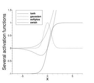
Figure 2: Profiles of several commonly-used activation functions.

Remark 2.1.

The parameter $S_{c}$ controls the minimum size of the random sub-interval $[t_{\min},t_{\max}]$. As $S_{c}\rightarrow 0$, random intervals with a near-zero size may be generated. This will cause the mapped synaptic input (and also the neuron response) to cluster around a constant level, which will affect the accuracy adversely. On the other hand, as $S_{c}\rightarrow 2S_{b}$, all the random sub-intervals $[t_{\min},t_{\max}]\rightarrow[-S_{b},S_{b}]$. So the randomness in the sub-interval will be lost, and the accuracy will deteriorate as mentioned before. We observe from numerical experiments that a value around $S_{c}=S_{b}/2$ produces results with very good (and oftentimes the best) accuracy. So in the current paper we will employ $S_{c}=S_{b}/2$ with modBIP in the numerical simulations.

Remark 2.2.

The parameter $S_{b}$ controls which regime the pre-training algorithm generally maps the synaptic input data into. If $S_{b}$ is very small, the mapped synaptic input will be close to zero, and many activation functions are close to a linear function in this regime. Since a linear function reduces the approximation capability of a neuron, the accuracy in this case will be limited. If $S_{b}$ is very large, the magnitude of the mapped synaptic input to the neuron can be large. It is thus more likely to cause saturation in the neuron response, which is unfavorable for the information transmission and can have an adverse effect on the accuracy. Figure 2 shows the profiles of several commonly-used activation functions, including the $\tanh$, Gaussian ($\sigma(x)=e^{-x^{2}}$), softplus ($\sigma(x)=\log(1+e^{x})$), and swish ($\sigma(x)=x/(1+e^{-x})$) functions. They suggest that a reasonable range for the input to the activation function seems to be somewhere around $[-3,3]$, and perhaps even a little larger with the swish and softplus functions. We observe from numerical experiments that, with the $\tanh$ (and Gaussian) activation function and a single hidden layer in the neural network, a value around $S_{b}=2\sim 3$ will produce results with good accuracy. For certain problems, the method achieves even better accuracy if $S_{b}$ is adjusted from this base value. When the neural network contains more hidden layers, it is observed that $S_{b}$ should typically be decreased from this reference range to achieve a better accuracy.

While the above reference range for $S_{b}$ is useful, for a given problem can we estimate the $S_{b}$ value that provides the best or close to the best accuracy? The answer is positive, and we next outline a procedure for estimating the optimal $S_{b}$ using simple numerical experiments. Let us use the problem of solving linear PDEs for illustration. When training the ELM neural network, suppose the linear system resulting from the PDE that one needs to solve using the least squares method is given by the following (see Section 2.3),

$$\mathbf{A}\mathbf{x}=\mathbf{b}$$ (6)

where $\mathbf{A}$, $\mathbf{x}$, and $\mathbf{b}$ denote the coefficient matrix (non-square), the vector of unknowns, and the right-hand-side vector, respectively. Let $\mathbf{r}$ denote the residual vector associated with the least squares solution,

$$\mathbf{r}=\mathbf{b}-\mathbf{A}\mathbf{x}^{+},$$ (7)

where $\mathbf{x}^{+}$ denotes the least squares solution to equation (6) (with minimum norm if rank-deficient). We use the residual norm $\|\mathbf{r}\|$ as an indicator to the accuracy of the least squares solution. Since $\|\mathbf{r}\|$ can be readily evaluated, we will use preliminary simulations to compute $\|\mathbf{r}\|$ and estimate the best $S_{b}$. The main steps are as follows:

• Consider a set of points from a range for $S_{b}$ (e.g. $S_{b}\in[0.5,5]$).

• For each $S_{b}$ value, set $S_{c}=S_{b}/2$ and pre-train the random coefficients of the network using modBIP.

• Perform a preliminary ELM simulation using the pre-trained neural network, and compute $\|\mathbf{r}\|$.

• Collect $\|\mathbf{r}\|$ for the set of $S_{b}$ values. Find the $S_{b}$ corresponding to the smallest (or close to the smallest) $\|\mathbf{r}\|$. Use this value as an estimate for the best $S_{b}$.

With the estimate for $S_{b}$ available, we can then use it in modBIP and perform actual simulations for the given problem with ELM. It should be noted that in the simulations for estimating $S_{b}$, the number of training data points should be larger than the number of training parameters in the neural network to avoid the regime of rank deficiency in the least squares solution.

Remark 2.3.

In the current work we have considered a symmetric interval $[-S_{b},S_{b}]$ in the modBIP algorithm. For activation functions that are not symmetric or anti-symmetric (e.g. swish, softplus), one can imagine that the use of a non-symmetric interval such as $[S_{b1},S_{b2}]$ in the algorithm might be more favorable. This aspect is not considered here, and we employ a symmetric interval in the current work.

Remark 2.4.

We observe that the ELM method, with the random coefficients pre-trained by the current modBIP algorithm, produces highly accurate simulation results, and that the accuracy of the combined ELM/modBIP method is insensitive to the random coefficient initializations. More specifically, with the hidden-layer coefficients initialized as random values generated on $[-R_{m},R_{m}]$, for an arbitrary $R_{m}$, the combined ELM/modBIP method produces accurate results and the accuracy is insensitive to $R_{m}$. This is very different from the behavior of ELM without pre-training of the random coefficients (see e.g. Figure 1). We will demonstrate this point with numerical experiments in Section 3.

Remark 2.5.

It is evident that the modBIP algorithm does not involve the activation function in its construction. Therefore, essentially any activation function can be used in the neural network together with the current method. This is in sharp contrast with the BIP algorithm NeumannS2013 , which employs the inverse of the activation function in its construction. BIP requires the activation functions in the neural network to be invertible (i.e. monotonic). This precludes many often-used activation functions such as the Sigmoid weighted linear unit (SiLU or swish) ElfwingUD2018 , Gaussian error linear unit (GELU) HendrycksG2020 , Gaussian, and other radial basis-type functions.

Remark 2.6.

We briefly mention another method for generating target samples from a normal distribution, which is different from what has been discussed above. In Algorithm 1 we replace the constant $S_{c}$ by two constants $S_{c_{1}}$ and $S_{c_{2}}$, with $0<S_{c_{1}}\leqslant S_{c_{2}}$. So now there are three constant parameters in the input, $S_{b}$, $S_{c_{1}}$ and $S_{c_{2}}$. We replace the lines $12$ and $13$ of Algorithm 1 by the following steps for generating the random target samples $t_{i}$ ($1\leqslant i\leqslant N_{s}$):

$$\textnormal{generate a uniform random number}\ \mu\ \textnormal{on}\ [-S_{b},S_{b}];$$

$$\textnormal{generate a uniform random number}\ \delta\ \textnormal{on}\ [S_{c_{1}},S_{c_{2}}];$$

$$\textnormal{generate random numbers}\ t_{i}\ (1\leqslant i\leqslant N_{s})\ \textnormal{from a normal distribution with mean}=\mu,\ \textnormal{stddev}=\delta.$$

Here we use a random mean $\mu$ from $[-S_{b},S_{b}]$ and a random standard deviation $\delta$ from $[S_{c_{1}},S_{c_{2}}]$ for generating the target samples $t_{i}$. We observe that a value around $S_{b}=2\sim 2.5$, $S_{c_{1}}=0.2$ and $S_{c_{2}}=S_{b}/2$ generally produce results with good accuracy.

2.3 Solving Linear Differential Equations with Combined ELM/modBIP

We will test the modBIP pre-training algorithm by combining it with ELM for solving linear partial differential equations. We first initialize the hidden-layer coefficients in the neural network by uniform random values from $[-R_{m},R_{m}]$, for some prescribed $R_{m}$. Then we pre-train these random coefficients by modBIP, and afterwards fix the updated hidden-layer coefficients. At this point, we can use the ELM method and the pre-trained neural network in the usual fashion. We can compute the training parameters (output-layer coefficients) by a linear least squares method for solving linear partial differential equations. This will be discussed in this subsection.

The use of ELM for solving linear partial differential equations has been discussed in a number of previous works; see e.g. PanghalK2020 ; DwivediS2020 ; DongL2020 and the references therein. For the sake of completeness, we summarize the main procedure below, and we refer the reader to e.g. DongL2020 for more detailed discussions of related aspects. Here we assume that the hidden-layer coefficients of the neural network have been pre-trained by modBIP as discussed above. So the weight/bias coefficients in the hidden layers are fixed throughout the computations to be discussed below.

For illustration we consider a rectangular domain in two dimensions (2D), $\Omega=\{(x,y)\ |\ x\in[a_{1},a_{2}],\ y\in[b_{1},b_{2}]\}$. If the problem is time-dependent, we will treat the time $t$ in the same way as the spatial variables, and use the last independent variable to denote the time $t$. In the case with two independent variables, for time-dependent problems, the last independent variable (i.e. $y$) denotes the time $t$. With this notation, we can treat time-dependent and time-independent problems in a unified fashion. So the following discussions also apply to time-dependent problems.

Consider a generic linear partial differential equation on $\Omega$,

$$\mathbf{L}u=f(x,y),$$ (8a)

$$\mathbf{B}u=g(x,y),\quad\text{on}\ \partial\Omega,$$ (8b)

where $u(x,y)$ is the field function to be solved for, $\mathbf{L}$ is a linear differential operator, $\mathbf{B}$ is a linear operator, $f(x,y)$ is a prescribed source term on the domain, and $g(x,y)$ is a prescribed source term defined on the domain boundary $\partial\Omega$. We assume that the system as given by (8a)–(8b) is well-posed. Note that, depending on the order of $\mathbf{L}$, the boundary condition (8b) may be imposed only on a part of the domain boundary, and that it should include the initial condition(s) if this is a time-dependent problem.

To solve equations (8a)–(8b), we use an extreme learning machine (feed-forward neural network), with its random hidden-layer coefficients pre-trained by modBIP, to represent the solution field $u(x,y)$. The input layer of the neural network consists of two nodes, representing $x$ and $y$, respectively. The output layer of the neural network consists of one node, representing the solution $u$. The neural network contains one or multiple hidden layers in between. Let $M$ denote the number of nodes in the last hidden layer of the neural network, and let $V_{j}(x,y)$ ($1\leqslant j\leqslant M$) denote the output fields of the last hidden layer. Then the logic of the output layer is given by

$$u(x,y)=\sum_{j=1}^{M}\beta_{j}V_{j}(x,y),$$ (9)

where $\beta_{j}$ ($1\leqslant j\leqslant M$) denote the weight coefficients in the output layer, which are the training parameters of the neural network.

We employ $(Q_{x}+1)$ and $(Q_{y}+1)$ uniform grid points in the $x$ and $y$ directions, respectively, with their coordinates given by

$$x_{p}=a_{1}+\frac{a_{2}-a_{1}}{Q_{x}}p,\quad y_{q}=b_{1}+\frac{b_{2}-b_{1}}{Q_{y}}q,\quad 0\leqslant p\leqslant Q_{x},\quad 0\leqslant q\leqslant Q_{y}.$$ (10)

We enforce the equation (8a) on all the grid points $(x_{p},y_{q})$, which will be refer to as the collocation points, and arrive at

$$\sum_{j=1}^{M}\left[\mathbf{L}V_{j}(x_{p},y_{q})\right]\beta_{j}=f(x_{p},y_{q}),\quad 0\leqslant p\leqslant Q_{x},\quad 0\leqslant q\leqslant Q_{y},$$ (11)

where equation (9) has been employed. Let $X_{b}$ denote the set of collocation points, among $(x_{p},y_{q})$, that reside on the domain boundary $\partial\Omega$ where the boundary condition (8b) is imposed on. Let $Q_{b}$ denote the number of points in $X_{b}$. We enforce the boundary condition (8b) on each $(x^{\prime}_{m},y^{\prime}_{m})\in X_{b}$, and arrive at

$$\sum_{j=1}^{M}[\mathbf{B}V_{j}(x^{\prime}_{m},y^{\prime}_{m})]\beta_{j}=g(x^{\prime}_{m},y^{\prime}_{m}),\quad 0\leqslant m\leqslant Q_{b}-1.$$ (12)

Equations (11) and (12) form a linear algebraic system about the training parameters $\beta_{j}$ ($1\leqslant j\leqslant M$). This system consists of $[(Q_{x}+1)(Q_{y}+1)+Q_{b}]$ equations and $M$ unknowns. The terms involved in the coefficient matrix, such as $V_{j}(x_{p},y_{q})$, $\mathbf{L}V_{j}(x_{p},y_{q})$, $V_{j}(x^{\prime}_{m},y^{\prime}_{m})$ and $\mathbf{B}V_{j}(x^{\prime}_{m},y^{\prime}_{m})$, can be computed by a forward evaluation of the neural network or by auto-differentiation. We seek a least squares solution (with minimum norm if the problem is rank deficient) to this system, and solve it by the linear least squares method GolubL1996 . In the current implementation, we have employed the linear least squares routine from LAPACK, available through the wrapper function in the scipy package in Python (function scipy.linalg.lstsq).

In the current paper, we implement the neural network in Python employing the Tensorflow and Keras libraries. The neural-network layers are implemented as the “Dense” layers in Keras. The input (training) data to the neural network consist of the coordinates of all the collocation points $(x_{p},y_{q})$ ($0\leqslant p\leqslant Q_{x}$ and $0\leqslant q\leqslant Q_{y}$) in the domain. In our implementation, we have incorporated an affine mapping between the input layer and the first hidden layer to normalize the input $(x,y)$ data from $\Omega=[a_{1},a_{2}]\times[b_{1},b_{2}]$ to the domain $[-1,1]\times[-1,1]$. This mapping is implemented by a “lambda” layer in Keras, which contains no weight/bias coefficients. This lambda layer does not need to be pre-trained by modBIP. With this lambda layer incorporated, in line $3$ of Algorithm 1, $\bm{\Phi}_{l-1}$ should be the output of the lambda layer, i.e. the normalized data, instead of the original input data $\mathbf{X}$.

After the linear system consisting of (11) and (12) is solved by the linear least squares method, the weight coefficients of the output layer will be set to the computed solution. Then the neural network is evaluated on a set of finer grid points, which is different from the training data points, to attain the field solution data $u(x,y)$. The solution data is then compared with e.g. the exact solution to compute the errors and other useful quantities. These steps have been followed in the numerical experiments of Section 3.

Remark 2.7.

For longer-time simulations of time-dependent partial differential equations, we employ the block time-marching scheme developed in DongL2020 . The spatial-temporal domain is first divided into a number of windows along the time (time blocks). The equations (11) and (12) are solved on each time block, individually and successively, using the method discussed in this sub-section. After one time block is computed, the solution at the last time instant will be evaluated, and used as the initial condition for the computation of the time block that follows. We refer to DongL2020 for more detailed discussions of this scheme. Block time marching has been employed for simulations of time-dependent problems in Section 3.

3 Representative Numerical Examples

In this section we evaluate the performance of the modBIP algorithm using function approximation and linear partial differential equations in one or two dimensions (1D/2D) in space, and plus time if the problem is time-dependent. We solve these equations numerically by the combined ELM/modBIP method as discussed in Section 2.3. The random hidden-layer coefficients in the neural network are pre-trained by modBIP first, and then they are fixed and used in ELM for finding the solutions to the differential equations. In the numerical experiments reported below, with modBIP we employ $S_{c}=S_{b}/2$, and estimate $S_{b}$ using the procedure outlined in Remark 2.2 by computing the residual norm of the linear least squares (LLSQ) problem in ELM. When generating the target samples on the random interval $[t_{\min},t_{\max}]$, we have employed the normal distribution with a mean $(t_{\min}+t_{\max})/2$ and a standard deviation $(t_{\max}-t_{\min})/4$ (see line $13$ of Algorithm 1) in all the numerical tests. The numerical experiments are conducted on a MAC computer (3.2GHz Quad-Core Intel Core i5 CPU, 24GB memory) in the authors’ institution. The wall clock time is collected by using the “timeit” module in Python.

In the current implementation, the initial random coefficients in the hidden layers are generated using the random number generator from the Tensorflow library (invoked by the initialization routines in the Keras library), while the random values in the modBIP algorithm are generated by the random number generator in the numpy package in Python. In order to make all the simulation results reported here fully repeatable, we have employed the same seed value for the random number generators in both Tensorflow and numpy, and the seed value is fixed for all the numerical experiments reported within a subsection. More specifically, the seed value is $1$ for the numerical experiments presented in Sections 3.1 and 3.2, $12$ for those in Section 3.3, and $22$ for those in Section 3.4, respectively.

Hereafter we employ the vector $[M_{0},M_{1},\dots,M_{L}]$ ($L\geqslant 2$) to represent the architecture of the feed-forward neural network in ELM, where the vector length $(L+1)$ denotes the number of layers in the network and $M_{i}$ is the number of nodes in layer $i$ for $0\leqslant i\leqslant L$. Note that $M_{0}$ and $M_{L}$ are the numbers of nodes in the input and output layers, respectively. The number of training parameters in ELM is $M_{L-1}$, i.e. the number of nodes in the last hidden layer, as discussed in Section 2.

3.1 Function Approximation

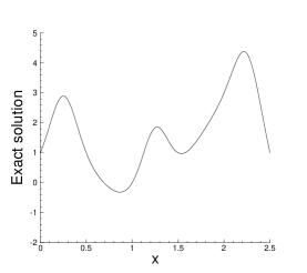
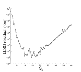
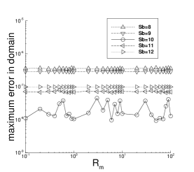
(a) (b) (c)

Figure 3: Function approximation: (a) Distribution of the exact function. (b) Residual norm of the linear least squares (LLSQ) problem versus $S_{b}$, for estimating the best $S_{b}$ in modBIP. (c) The maximum error of the ELM/modBIP solution as a function of $R_{m}$, corresponding to several $S_{b}$ in modBIP.

We approximate the following function $u(x)$ by the combined ELM/modBIP method,

$$u=e^{\sin(2\pi x)}+x\cos(\pi x),\quad x\in\left[0,2.5\right].$$ (13)

Figure 3(a) shows the distribution of this function on the domain. Note that the function approximation problem is equivalent to solving the linear PDE (8a), with no boundary condition, in which $\mathbf{L}$ is given by the identity operator and $f$ is given by the function to be approximated.

Let us first consider a single hidden layer in the neural network, with the network architecture given by $[1,100,1]$ and $\tanh$ as the activation function in the hidden layer (the output layer is linear). The input node represents $x$, and the output node represents the function $u(x)$. The input data to the neural network consists of $Q=121$ uniform grid (collocation) points on $[0,2.5]$; see equation (10) when restricted to 1D. The function values on these collocation points are provided in equation (8a) as the data for the source term. The hidden-layer coefficients are initialized by uniform random values generated on $[-R_{m},R_{m}]$, with $R_{m}$ specified below.

We first estimate the $S_{b}$ in modBIP using the procedure from Remark 2.2. Figure 3(b) shows the residual norm of the linear least squares (LLSQ) problem as a function of $S_{b}$ in a set of preliminary simulations. Here the initial random coefficients in the neural network are generated with $R_{m}=50$. They are pre-trained by modBIP, with $S_{c}=S_{b}/2$ and $S_{b}$ from a range of values. The residual norm of the LLSQ problem in ELM is collected corresponding to these $S_{b}$ values and plotted in Figure 3(b). This plot indicates that, while the residual norm at times fluctuates with respect to $S_{b}$, it achieves a relatively low level for a range of $S_{b}\approx 10\sim 20$ for this problem. We employ $S_{b}=10$ in modBIP in the majority of subsequent tests for this problem.

Figure 3(c) illustrates the general behavior of the ELM approximation error, with the random coefficients pre-trained by modBIP. It shows the maximum error in the domain of the ELM approximant as a function of $R_{m}$, the maximum magnitude of the initial random coefficients, corresponding to several $S_{b}$ values around $S_{b}=10$ in the modBIP algorithm. Here for a given $S_{b}$ value, we vary $R_{m}$ systematically in the range $0.1\leqslant R_{m}\leqslant 100$, and for each $R_{m}$ we initialize the hidden-layer coefficients by uniform random values generated on $[-R_{m},R_{m}]$ and pre-train the random coefficients by modBIP with the given $S_{b}$ and $S_{c}=S_{b}/2$. The pre-trained random coefficients are then used in ELM to compute the training parameters (i.e. the output-layer coefficients) by the linear least squares method for approximating the function (13). So the approximation function is now represented by the fully trained neural network. We then evaluate the trained neural network on a set of $401$ (finer) uniform grid points to compute the approximant values, which are then compared with the exact function (13) to attain the errors. We can observe from Figure 3(c) that, with the modBIP pre-training of the random coefficients, the ELM error is essentially independent of $R_{m}$, although some fluctuations with respect to $R_{m}$ can be observed in certain cases. This insensitivity to $R_{m}$ is a common characteristic of the combined ELM/modBIP method, which will be observed repeatedly in subsequent numerical experiments.

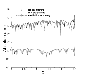
Figure 4: Function approximation: Distributions of the absolute error of the ELM approximant obtained with (a) no pre-training, (b) BIP pre-training, and (c) modBIP pre-training of the random coefficients.

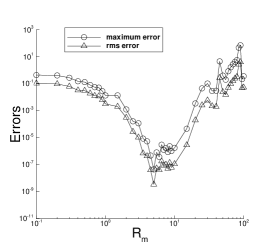
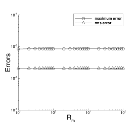
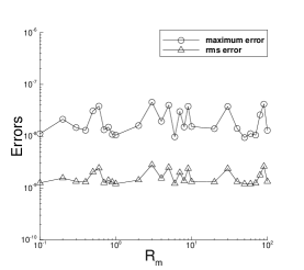
(a) (b) (c)

Figure 5: Function approximation: The maximum and rms errors in the domain of the ELM approximant as a function of $R_{m}$, attained with (a) no pre-training, (b) BIP pre-training, and (c) modBIP pre-training of the random coefficients.

Figures 4 and 5 are comparisons of the ELM errors of the function approximation problem obtained with three configurations: no pre-training of the random coefficients, and with pre-training of the random coefficients by the BIP algorithm NeumannS2013 and by the current modBIP algorithm. As mentioned before, the network architecture is characterized by $[1,100,1]$, with the $\tanh$ activation function and $Q=121$ uniform collocation points as the training data points. In this set of tests the initial random coefficients are generated with $R_{m}$ either fixed at $R_{m}=50$ or varied systematically. In the case without pre-training, the initial random coefficients are directly used in ELM for computing the training parameters and the approximation function. In the cases with pre-training, the initial random coefficients are pre-trained by BIP or modBIP first, and the pre-trained hidden-layer coefficients are then used in ELM for computing the approximation function. With BIP, we employ a normal distribution for generating the target samples for each hidden-layer node, with a random mean from $[-1,1]$ and a standard deviation $0.5$, as described in NeumannS2013 . The inverse of $\tanh$ is then applied to the target samples, which are then used to compute the mapping coefficients in BIP NeumannS2013 . With modBIP pre-training, we employ $S_{c}=S_{b}/2$ and $S_{b}=10$ in Algorithm 1.

Figure 4 compares profiles of the absolute error of the ELM approximant obtained without pre-training, with BIP pre-training, and with modBIP pre-training of the random coefficients. The initial random coefficients are generated with $R_{m}=50$ in this set of tests. The error levels of the ELM result with BIP pre-training and without pre-training are largely comparable, both on the order of $10^{-3}$. In contrast, the error level of the ELM result with the modBIP pre-training is considerably lower, on the order of $10^{-9}$. This indicates that the combined ELM/modBIP method is markedly more accurate than the ELM methods without pre-training and with the BIP pre-training of the random coefficients.

Figure 5 shows the maximum and root-mean-squares (rms) errors in the domain of the ELM approximants obtained without pre-training and with BIP and modBIP pre-training of the random coefficients. In this set of tests, $R_{m}$ is varied systematically between $0.1$ and $100$, and the maximum/rms errors of the ELM solution corresponding to the initial random coefficients generated on $[-R_{m},R_{m}]$, with and without pre-training, are computed and collected. Without pre-training of the random coefficients, the ELM accuracy exhibits a strong dependence on $R_{m}$. It produces quite accurate results in a range of moderate $R_{m}$ values, while outside this range the accuracy can be quite poor; see Figure 5(a). With BIP and modBIP pre-training of the random coefficients, the error of the ELM result is observed to be largely independent of $R_{m}$. The ELM error level corresponding to the modBIP pre-training is considerably smaller than that of the BIP pre-training (see Figures 5(b,c)).

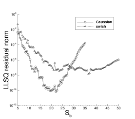
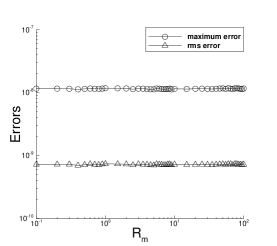
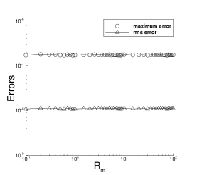
(a) (b) (c)

Figure 6: Function approximation (non-monotonic activation functions): (a) Residual norm of the LLSQ problem versus $S_{b}$, for estimating the best $S_{b}$ in modBIP. The maximum and rms errors of the ELM solution as a function of $R_{m}$ obtained using (b) the Gaussian and (c) the swish activation functions, with the random coefficients pre-trained by modBIP.

A prominent advantage of modBIP over BIP lies in that modBIP does not place any constraint on the activation function, while BIP requires the activation function to be invertible. So modBIP can be applied with many activation functions with which BIP breaks down. Two such examples are provided in Figure 6, with the Gaussian and the swish ElfwingUD2018 activation functions. Neither of these two functions has an inverse. Here the neural network has the same architecture as before, but the activation function for the hidden layer has been changed to the Gaussian function ($\sigma(x)=e^{-x^{2}}$) or the swish function ($\sigma(x)=x/(1+e^{-x})$). The initial random coefficients are generated with a fixed $R_{m}=50$ (plot (a)) or a varying $R_{m}$ (plots (b,c)), and pre-trained by modBIP. We employ the same training data points as before ($Q=121$), and $S_{c}=S_{b}/2$ in modBIP. Figure 6(a) shows the LLSQ residual norms for estimating the best $S_{b}$, suggesting a value around $S_{b}\approx 20$ with the Gaussian function and around $S_{b}\approx 24$ with the swish function. Figures 6(b,c) show the maximum and rms errors in the domain of the ELM/modBIP approximant as a function of $R_{m}$, corresponding to the Gaussian activation function (with $S_{b}=20$) and to the swish activation function (with $S_{b}=24$). The ELM/modBIP results exhibit a high accuracy (error level around $10^{-10}\sim 10^{-7}$), which is insensitive to $R_{m}$ (or the initial random coefficients). It should be noted that the BIP algorithm breaks down when used with these activation functions, because they do not have an inverse.

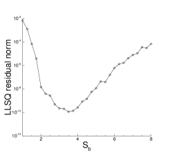
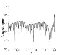
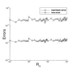
(a) (b) (c)

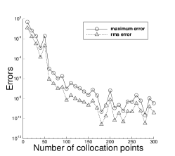
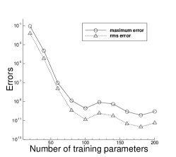
(d) (e)

Figure 7: Function approximation (3 hidden layers in neural network): (a) The LLSQ residual norm versus $S_{b}$, for estimating the best $S_{b}$ in modBIP. (b) Distribution of the absolute error of the ELM/modBIP approximant. The maximum/rms errors of the ELM/modBIP approximant as a function of (c) $R_{m}$, (d) the number of collocation points $Q$, and (e) the number of training parameters $M$. $Q$ is fixed at $Q=150$ in (a,b,c,e) and varied in (d). $M$ is fixed at $M=100$ in (a,b,c,d) and varied in (e). $R_{m}$ is fixed at $R_{m}=50$ in (a,b,d,e) and varied in (c). $S_{b}$ is varied in (a) and fixed at $S_{b}=3.5$ in (b,c,d,e).

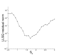
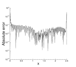
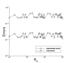
(a) (b) (c)

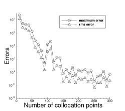
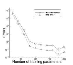
(d) (e)

Figure 8: Function approximation (7 hidden layers in neural network): (a) The LLSQ residual norm versus $S_{b}$, for estimating the best $S_{b}$ in modBIP. (b) Distribution of the absolute error of the ELM/modBIP approximant. The maximum/rms errors of the ELM/modBIP approximant as a function of (c) $R_{m}$, (d) the number of collocation points $Q$, and (e) the number of training parameters $M$. $Q$ is fixed at $Q=150$ in (a,b,c,e) and varied in (d). $M$ is fixed at $M=100$ in (a,b,c,d) and varied in (e). $R_{m}$ is fixed at $R_{m}=50$ in (a,b,d,e) and varied in (c). $S_{b}$ is varied in (a) and fixed at $S_{b}=1.7$ in (b,c,d,e).

The results presented so far are obtained with a single hidden layer in the neural network. Let us next investigate the performance of the ELM/modBIP method with neural networks containing multiple hidden layers. Figures 7 and 8 display ELM/modBIP results obtained with $3$ and $7$ hidden layers in the neural network, respectively. The network architecture is characterized by the vectors $[1,40,40,M,1]$ and $[1,40,40,40,40,40,40,M,1]$ in these two cases, respectively, where $M$ denotes the number of training parameters and is either fixed at $M=100$ or varied between $M=20$ and $M=200$. The activation function is $\tanh$ in all hidden layers, and the output layer is linear. We employ $Q$ uniform grid (collocation) points in the domain as the training data points, with $Q$ either fixed at $Q=150$ or varied between $Q=10$ and $Q=300$. The initial hidden-layer coefficients are set to uniform random values generated on $[-R_{m},R_{m}]$, with $R_{m}$ either fixed at $R_{m}=50$ or varied between $R_{m}=0.1$ and $R_{m}=100$. These initial random coefficients are pre-trained by modBIP with $S_{c}=S_{b}/2$.

Figure 7 illustrates the ELM/modBIP results with three hidden layers in the neural network. The plot (a) shows the LLSQ residual norms for estimating the best $S_{b}$ in modBIP, suggesting a value around $S_{b}\approx 3.5$. The plot (b) depicts the error distribution of the ELM/modBIP approximant against the actual function (13). The plots (c,d,e) show the maximum and rms errors in the domain of the ELM/modBIP appximant as a function of $R_{m}$, the number of training collocation points $Q$, and the number of training parameters $M$. The specific parameter values employed for each plot are provided in the caption of Figure 7.

Figure 8 shows the corresponding ELM/modBIP results obtained with seven hidden layers in the neural network. The LLSQ residual norms in plot (a) suggest a value around $S_{b}\approx 1.7$ for modBIP, which has been employed to attain the error distribution and the maximum/rms errors of the ELM/modBIP in the plots (b) to (e). The specific parameter values for each case are provided in the caption of this figure.

The results in Figures 7 and 8 indicate that the combined ELM/modBIP method produces highly accurate results with multiple hidden layers in the neural network. The best $S_{b}$ for modBIP (with $S_{c}=S_{b}/2$) appears to decrease with increasing number of hidden layers in the neural network. The ELM/modBIP errors are not sensitive to the initial random coefficients, similar to what has been observed with a single hidden layer in the network. These errors decrease approximately exponentially as the number of collocation points or the number of training parameters increases, until they essentially saturate when the number of collocation points or training parameters becomes sufficiently large.

3.2 Poisson Equation

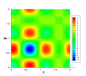
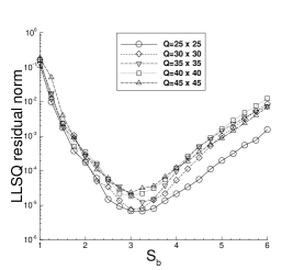
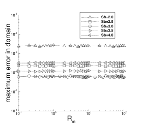
(a) (b) (c)

Figure 9: Poisson equation: (a) Distribution of the exact solution. (b) LLSQ residual norm as a function of $S_{b}$, for estimating the best $S_{b}$ in modBIP. (c) The maximum error of the ELM/modBIP solution as a function of $R_{m}$. $R_{m}=10$ in (b) and is varied in (c). $Q=25\times 25$ in (c), and takes several values in (b). $S_{b}$ takes several values in (c), and is varied in (b).

We next consider the two-dimensional (2D) domain $\Omega=\{(x,y)\ |\ x\in[0,2],\ y\in[0,2]\}$, and test the combined ELM/modBIP method using the boundary value problem with the Poisson equation on $\Omega$:

$$\frac{\partial^{2}u}{\partial x^{2}}+\frac{\partial^{2}u}{\partial y^{2}}=f(x,y),$$ (14a)

$$u(0,y)=g_{1}(y),$$ (14b)

$$u(2,y)=g_{2}(y),$$ (14c)

$$u(x,0)=h_{1}(x),$$ (14d)

$$u(x,2)=h_{2}(x),$$ (14e)

where $u(x,y)$ is the field function to be solved for, $f(x,y)$ is a prescribed source term, and $g_{1}$, $g_{2}$, $h_{1}$ and $h_{2}$ are the Dirichlet boundary distributions. We consider the following manufactured solution to this problem,

$$u(x,y)=-\left[\frac{3}{2}\cos\left(\pi x+\frac{7\pi}{20}\right)+2\cos\left(2\pi x-\frac{\pi}{4}\right)\right]\left[\frac{3}{2}\cos\left(\pi y+\frac{7\pi}{20}\right)+2\cos\left(2\pi y-\frac{\pi}{4}\right)\right].$$ (15)

Accordingly, the source term $f$ and the boundary distributions are chosen such that the expression (15) satisfies the system (14). Figure 9(a) illustrates the distribution of this analytic solution.

We employ the combined ELM/modBIP method to solve the system (14); see Section 2.3. We first consider a single hidden layer in the neural network, with an architecture given by $[2,500,1]$, the $\tanh$ activation function for the hidden layer, and a linear output layer. The input layer ($2$ nodes) represents the coordinates $x$ and $y$, and the output layer ($1$ node) represents the field solution $u(x,y)$. We employ a set of $Q=25\times 25$ uniform grid (collocation) points as the training data points, i.e. with $25$ points in both $x$ and $y$ directions (see equation (10)), which constitute the input data into the neural network. The hidden-layer coefficients in the neural network are initialized to uniform random values generated on $[-R_{m},R_{m}]$, with $R_{m}$ either fixed at $R_{m}=10$ or varied between $R_{m}=0.1$ and $R_{m}=100$ in the following tests. The initial random coefficients are pre-trained by modBIP with $S_{c}=S_{b}/2$ and $S_{b}$ determined by the procedure given in Remark 2.2.

Figure 9(b) shows the residual norm of the linear least squares (LLSQ) problem as a function of $S_{b}$ in modBIP, where the initial random coefficients are generated with $R_{m}=10$. The results corresponding to $Q=25\times 25$ and several other sets of collocation points are included, which all suggest a value around $S_{b}\approx 3$ for modBIP. Figure 9(c) shows the maximum and rms errors in the domain of the ELM/modBIP solution as a function of $R_{m}$, corresponding to several $S_{b}$ values around $S_{b}=3$ in modBIP (with $S_{c}=S_{b}/2$), where $Q=25\times 25$ collocation points have been employed. The errors of the ELM/modBIP method can be observed to be insensitive to $R_{m}$ (or the initial random coefficients).

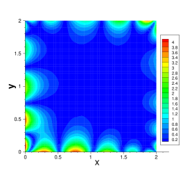
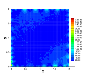
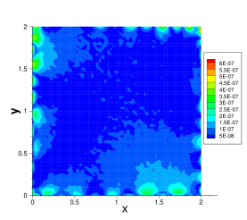
(b) (c) (d)

Figure 10: Poisson equation: Distributions of the absolute error of the ELM solution computed with (a) no pre-training, (b) BIP pre-training, and (c) modBIP pre-training of the random coefficients.

Figure 10 compares distributions of the absolute error of the ELM solution obtained with no pre-training and with the BIP and the modBIP pre-training of the random coefficients in the neural network. Here we have employed a network architecture given by $[2,500,1]$, the $\tanh$ activation function for the hidden layer, $Q=25\times 25$ uniform collocation points, and $R_{m}=10$ for generating the initial random coefficients. With BIP, we employ a normal distribution for the target samples, with a random mean generated on $[-1,1]$ from a uniform distribution and a standard deviation $0.5$ NeumannS2013 . With modBIP we employ $S_{b}=3$ and $S_{c}=S_{b}/2$ in the algorithm. One can observe that the ELM result is inaccurate without pre-training of the random coefficients. With both BIP and modBIP pre-training of the random coefficients, the ELM method produces accurate solutions to the Poisson equation. The ELM/modBIP solution is markedly more accurate than that of ELM/BIP.

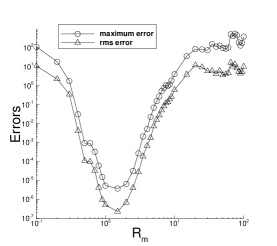
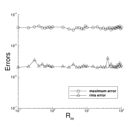
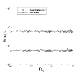
(a) (b) (c)

Figure 11: Poisson equation: the maximum and rms errors in the domain as a function of $R_{m}$, obtained with (a) no pre-training, (b) BIP pre-training, and (c) modBIP pre-training of the random coefficients.

Figure 11 is a further comparison of the cases with no pre-training and with BIP and modBIP pre-training of the random coefficients. Here we vary $R_{m}$ systematically, and for each $R_{m}$ we initialize the hidden-layer coefficients to uniform random values from $[-R_{m},R_{m}]$, which are then pre-trained by BIP or modBIP and used in the ELM computations. The other parameter values are identical to those for Figure 10. The three plots show the maximum and rms errors in the domain of the ELM solution as a function of $R_{m}$, obtained with no pre-training and with the BIP and modBIP pre-training of the random coefficients. With no pre-training, $R_{m}$ is observed to strongly influence the accuracy of the ELM solution. With both BIP and modBIP pre-training of the random coefficients, the accuracy of the ELM solution becomes essentially independent of $R_{m}$. The error level of the ELM/modBIP solution is markedly lower than that of the ELM/BIP solution.

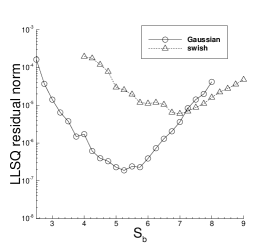
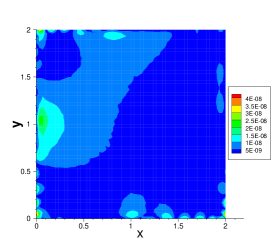
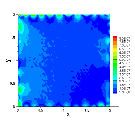
(a) (b) (c)

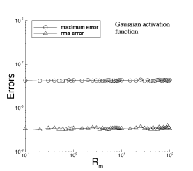
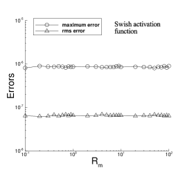
(d) (e)

Figure 12: Poisson equation (non-monotonic activation functions): (a) LLSQ residual norms versus $S_{b}$, for estimating the best $S_{b}$ in modBIP with the Gaussian and swish activation functions. Error distributions of the ELM/modBIP solution obtained with (b) Gaussian and (c) swish activation functions. Maximum/rms errors of the ELM/modBIP solution versus $R_{m}$, obtained with (d) Gaussian and (e) swish activation functions. $R_{m}=10$ in (a,b,c) and is varied in (d,e). $S_{b}=5$ in (b,d) and $S_{b}=7$ in (c,e).

Figure 12 illustrates the ELM/modBIP results attained with the Gaussian and the swish activation functions for the hidden layers. It should be noted that the BIP algorithm NeumannS2013 breaks down with these activation functions because they do not have an inverse. In these tests, we have employed a network architecture $[2,500,1]$, $Q=25\times 25$ uniform collocation points, either a fixed $R_{m}=10$ or a varying $R_{m}$ for generating the initial random coefficients, and $S_{c}=S_{b}/2$ in modBIP. Figure 12(a) shows the LLSQ residual norms for estimating the $S_{b}$ parameter in modBIP, which suggest a value around $S_{b}\approx 5$ with the Gaussian function and a value around $S_{b}\approx 7$ with the swish function. Figures 12(b) and (d) show the error distribution of the ELM/modBIP solution with $R_{m}=10$, and its maximum/rms errors corresponding to the initial random coefficients generated with different $R_{m}$, computed using the Gaussian activation function with $S_{b}=5$ in modBIP. Figures 12(c) and (e) show the corresponding ELM/modBIP results computed using the swish activation function with $S_{b}=7$ in modBIP. These data indicate that the combined ELM/modBIP method produces highly accurate results with these activation functions, and that its accuracy is insensitive to the initial random coefficients.

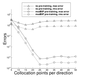
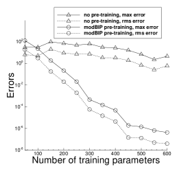
(a) (b)

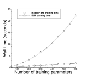
(c) (d)

Figure 13: Poisson equation: The maximum/rms errors of the ELM/modBIP solution as a function of (a) the number of collocation points in each direction and (b) the number of training parameters, attained with no pre-training and with modBIP pre-training of the random coefficients. The modBIP pre-training time of the random coefficients, and the ELM training time of the neural network, as a function of (c) the number of collocation points in each direction and (d) the number of training parameters.

Figure 13 compares the accuracy of the combined ELM/modBIP method and the ELM method with no pre-training of the random coefficients, and also examines the computational cost of the modBIP pre-training of the random coefficients. In this set of tests, we employ a neural network architecture $[2,M,1]$, where the number of training parameters $M$ is either fixed at $M=500$ or varied between $M=50$ and $M=600$. We employ the $\tanh$ activation function for the hidden layer, and $Q=Q_{1}\times Q_{1}$ uniform collocation points in the domain, where $Q_{1}$ denotes the number of collocation points in $x$/$y$ directions and is either fixed at $Q_{1}=35$ or varied between $Q_{1}=5$ and $Q_{1}=50$. The initial random coefficients are generated with $R_{m}=10$, and we employ $S_{b}=3$ and $S_{c}=S_{b}/2$ in modBIP. Figure 13(a) shows the maximum and rms errors of the ELM solutions as a function of $Q_{1}$, obtained without pre-training and with modBIP pre-training of the random coefficients and with a fixed $M=500$. Figure 13(b) shows the maximum/rms ELM errors as a function of $M$, obtained with no pre-training and with modBIP pre-training and with a fixed $Q_{1}=35$ for the collocation points. The ELM solution obtained without pre-training the random coefficients generated with $R_{m}=10$ is not accurate, and increasing the number of collocation points or the training parameters results in little or no improvement in the accuracy. In contrast, the errors of the combined ELM/modBIP method decrease exponentially as the number of collocation points per direction $Q_{1}$ or the number of training parameters $M$ increases. The errors are observed to saturate at a level around $10^{-8}\sim 10^{-6}$ as $Q_{1}$ increase beyond $25$ for this case.

Figures 13(c) and (d) show the modBIP pre-training time of the random coefficients and the ELM training time of the neural network as a function of the number of collocation points in each direction ($Q_{1}$) and the number of training parameters ($M$), respectively. Both the modBIP pre-training time and the ELM network training time increase with increasing number of collocation points in the domain and increasing number of training parameters in the neural network. But the modBIP pre-training cost increases much more slowly than the latter. The modBIP pre-training cost of the random coefficients is only a fraction of the ELM network training cost. For example, in the range of collocation points tested here, the modBIP pre-training time is about $2\sim 10\%$ of the ELM network training time. These results suggest that the modBIP pre-training of the random coefficients is not significant in terms of the overhead it induces. It should be noted that the modBIP pre-training cost can be further reduced, because logically pre-training the random coefficients only needs to be performed once (the first time) for a given a network architecture and the input collocation points. The pre-trained hidden-layer random coefficients can be saved and used directly for subsequent ELM computations.

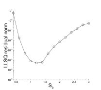
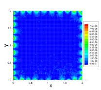
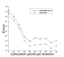
(a) (b) (c) (d)

Figure 14: Poisson equation ($3$ hidden layers in neural network): (a) LLSQ residual norms versus $S_{b}$, for estimating the best $S_{b}$ in modBIP. (b) Error distribution of the ELM/modBIP solution. Maximum/rms errors of the ELM/modBIP solution as a function of (c) $R_{m}$, and (d) the number of collocation points in each direction. $S_{b}=1$ in (b,c,d) and is varied in (a). $R_{m}=10$ in (a,b,d) and is varied in (c). $Q=25\times 25$ in (a,b,c) and is varied in (d). $M=500$ in (a,b,c,d).

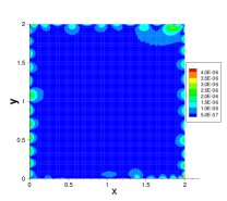
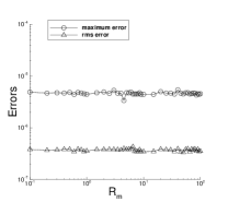
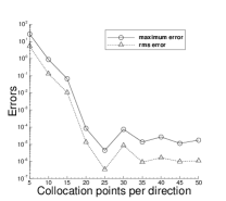
(a) (b) (c) (d)

Figure 15: Poisson equation (5 hidden layers in neural network): (a) LLSQ residual norm for estimating the best $S_{b}$ in modBIP. (b) Error distribution of the ELM/modBIP solution. The maximum/rms errors of ELM/modBIP solution as a function of (c) $R_{m}$, and (d) the number of collocation points in each direction. $S_{b}=0.8$ in (b,c,d) and is varied in (a). $R_{m}=10$ in (a,b,d) and is varied in (c). $Q=25\times 25$ in (a,b,c) and is varied in (d). $M=500$ in (a,b,c,d).

We next test the combined ELM/modBIP method for solving the Poisson equation with multiple hidden layers in the neural network. Figures 14 and 15 illustrate the ELM/modBIP simulation results obtained using neural networks containing $3$ hidden layers, with an architecture $[2,50,50,500,1]$, and $5$ hidden layers, with an architecture $[2,50,50,50,50,500,1]$, respectively. The activation function is $\tanh$ in the hidden layers. In these tests the initial random coefficients are generated on $[-R_{m},R_{m}]$ with $R_{m}$ either fixed at $R_{m}=10$ or varied between $R_{m}=0.1$ and $R_{m}=100$. We employ $Q=Q_{1}\times Q_{1}$ uniform collocation points, where $Q_{1}$ is fixed at $Q_{1}=25$ or varied between $Q_{1}=5$ and $Q_{1}=50$. In modBIP we employ $S_{c}=S_{b}/2$ and determine $S_{b}$ based on the procedure from Remark 2.2.

Figure 14(a) shows the LLSQ residual norms for estimating $S_{b}$, suggesting a value around $S_{b}\approx 1$ for modBIP with three hidden layers in the neural network. Figures 14(b) to (d) show the error distribution, and the maximum/rms errors in the domain of the ELM/modBIP solution as a function of $R_{m}$ and $Q_{1}$, obtained with $S_{b}=1$ in modBIP. The specific parameter values for each plot are provided in the caption of this figure. Figure 15(a) shows the LLSQ residual norms computed with $5$ hidden layers in the neural network, suggesting a value around $S_{b}\approx 0.8$ in this case. Figures 15(b,c,d) show the ELM/modBIP results obtained with $5$ hidden layers in the neural network and $S_{b}=0.8$ in modBIP, which correspond to those of Figures 14(b,c,d). These results confirm that the combined ELM/modBIP method produces accurate simulation results with multiple hidden layers in the neural network. The characteristics of exponential convergence and insensitivity to $R_{m}$ are similar to what has been observed with single-hidden-layer neural networks.

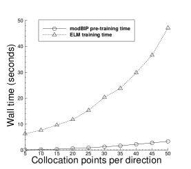
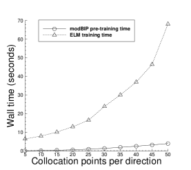
(a) (b)

Figure 16: Poisson equation: The modBIP pre-training time of the random coefficients and the ELM training time of the neural network as a function of the number of collocation points in each direction, obtained with $3$ hidden layers (a) and $5$ hidden layers (b) in the neural network. The network architecture of (a) is $[2,50,50,500,1]$ and the parameter values correspond to those of Figure 14(d). The network architecture of (b) is $[2,50,50,50,50,500,1]$ and the parameter values correspond to those of Figure 15(d).

Figure 16 is a study of the computational cost of the modBIP pre-training of the random coefficients and the ELM training of the neural network with multiple hidden layers in the neural network. It shows the modBIP pre-training time and the ELM network training time as a function of the number of collocation points in each direction, corresponding to $3$ and $5$ hidden layers in the neural network. The network architecture and the parameter values in Figures 16(a) and (b) are identical to those of Figure 14(d) and Figure 15(d), respectively. In the range of collocation points tested here, the modBIP pre-training cost is approximately $2\sim 8\%$ of the ELM network training cost with $3$ hidden layers, and approximately $2\sim 7\%$ of the ELM network training cost with $5$ hidden layers in the neural network.

3.3 Wave Equation

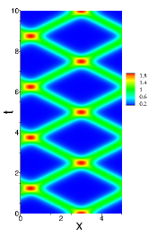
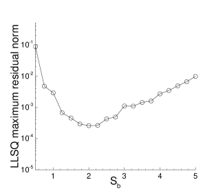
(a) (b) (c)

Figure 17: Wave equation: (a) Distribution of the exact solution in the spatial-temporal plane. (b) The maximum residual norm of the LLSQ problem versus $S_{b}$, for estimating the best $S_{b}$ in modBIP. (c) The maximum error in the overall domain as a function of $R_{m}$, corresponding to several $S_{b}$ values in modBIP for pre-training the random coefficients.

We next test the ELM/modBIP method using the one-dimensional second-order wave equation (plus time). Consider the spatial-temporal domain, $\Omega=\{(x,t)\ |\ x\in[0,5],\ t\in[0,10]\}$, and the initial/boundary-value problem with the wave equation on this domain,

$$\frac{\partial^{2}u}{\partial t^{2}}-c^{2}\frac{\partial^{2}u}{\partial x^{2}}=0,$$ (16a)

$$u(0,t)=u(5,t),$$ (16b)

$$\frac{\partial}{\partial x}u(0,t)=\frac{\partial}{\partial x}u(5,t),$$ (16c)

$$u(x,0)=2\operatorname{sech}^{3}\left[\frac{3}{\delta_{0}}(x-x_{0})\right],$$ (16d)

$$\left.\frac{\partial u}{\partial t}\right|_{(x,0)}=0,$$ (16e)

where $u(x,t)$ is the field solution to be solved for, periodic boundary conditions are imposed on $x=0$ and $5$, $c$ is the wave speed, $x_{0}$ is the initial peak location of the wave, and the constant $\delta_{0}$ controls the width of the wave profile. The constant parameters assume the following values for this problem:

$$c=2,\quad\delta_{0}=2,\quad x_{0}=3.$$

This problem has the following solution,

$$\left\{\begin{split}&u(x,t)=\operatorname{sech}^{3}\left[\frac{3}{\delta_{0}}\left(-\frac{5}{2}+\xi\right)\right]+\operatorname{sech}^{3}\left[\frac{3}{\delta_{0}}\left(-\frac{5}{2}+\eta\right)\right],\\ &\xi=\text{mod}\left(x-x_{0}+ct+\frac{5}{2},5\right),\quad\eta=\text{mod}\left(x-x_{0}-ct+\frac{5}{2},5\right),\end{split}\right.$$ (17)

where mod refers to the modulo operation. The two terms in this solution represent the leftward- and rightward-traveling waves, respectively. Figure 17(a) shows the distribution of this solution in the spatial-temporal plane.

To simulate this problem, we employ the block time-marching scheme and the local extreme learning machines (locELM) developed in DongL2020 . We first divide the spatial-temporal domain $\Omega$ along the temporal direction into $20$ uniform time blocks, and the system (16) is computed on each time block individually and successively (see Remark 2.7). We partition the spatial-temporal domain of each time block into $4$ uniform sub-domains along the $x$ direction, and represent the field solution $u(x,t)$ on each sub-domain by a local feed-forward neural network DongL2020 . $C^{1}$ continuity conditions are imposed on the sub-domain boundaries. The configuration of the local neural networks follows that of the ELM. The weight/bias coefficients in the hidden layers of the local neural networks are initialized as uniform random values generated on $[-R_{m},R_{m}]$, which are pre-trained by modBIP and then fixed afterwards. The output layers of the local neural networks are linear (with zero bias), and the weight coefficients therein are the training parameters and can be determined by a least squares computation. The local neural networks are coupled with one another due to the $C^{1}$ continuity conditions DongL2020 , and need to be trained together as a whole system. By enforcing the system of equations, boundary/initial conditions, and the $C^{1}$ continuity conditions on a set of collocation points inside each sub-domain and on the domain and sub-domain boundaries, we arrive at a system of linear algebraic equations about the training parameters, which can be solved by the linear least squares method. We refer to DongL2020 for more detailed discussions of the locELM method and the block time marching scheme.

After the random coefficients in the local neural networks are initialized, we use modBIP to pre-train the random coefficients in each local neural network (see Algorithm 1), and then employ the pre-trained random coefficients in the locELM computation for the training parameters based on the linear least squares method. We refer to the overall method as the combined locELM/modBIP method.

We first consider a single hidden layer in the local neural networks, whose architecture each is characterized by $[2,250,1]$ and with $\tanh$ as the activation function for the hidden layers. The two nodes in the input layer represent the spatial-temporal coordinates $x$ and $t$, and the single node in the output layer represents the field function $u(x,t)$ on the corresponding sub-domain. We employ $Q=25\times 25$ uniform collocation points on each sub-domain, and $S_{c}=S_{b}/2$ in the modBIP algorithm. $S_{b}$ in modBIP is determined by the procedure from Remark 2.2.

Figure 17(b) shows the maximum residual norms, among the $20$ time blocks, of the linear least squares (LLSQ) problem as a function of $S_{b}$, for estimating the best $S_{b}$ in modBIP. In this set of tests, the initial random coefficients are generated with $R_{m}=50$. The data suggest a value around $S_{b}\approx 2$ for modBIP. Figure 17(c) shows the maximum error in the entire spatial-temporal domain of the locELM/modBIP solution as a function of $R_{m}$, obtained with several $S_{b}$ values in modBIP. We observe the familiar insensitivity of the locELM/modBIP error with respect to $R_{m}$ (or the initial random coefficients) in the neural network.

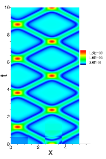
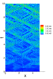
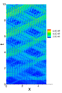
(a) (b) (c)

Figure 18: Wave equation: Distributions of the absolute error of the locELM solution obtained with (a) no pre-training, (b) BIP pre-training, and (c) modBIP pre-training of the random coefficients.

Figure 18 compares distributions in the spatial-temporal plane of the absolute error of the locELM solution obtained with no pre-training, and with BIP and modBIP pre-training of the random coefficients in the local neural networks. In this set of tests, we employ local neural networks with an architecture $[2,250,1]$, the $\tanh$ activation function for the hidden layers, and $Q=31\times 31$ uniform collocation points on each sub-domain. The initial random coefficients in the local neural networks are generated with $R_{m}=50$. With BIP, we generate target samples by a normal distribution with a random mean from $[-1,1]$ and a standard deviation $0.5$ NeumannS2013 . With modBIP we employ $S_{b}=2$ and $S_{c}=S_{b}/2$ in Algorithm 1. The locELM solution obtained without pre-training of the random coefficients generated by $R_{m}=50$ exhibits no accuracy for this problem (Figure 18(a)). On the other hand, the locELM solutions obtained with BIP and modBIP pre-training are quite accurate, and the combined locELM/modBIP solution is observed to be notably more accurate than the locELM/BIP one (with error levels $10^{-5}$ versus $10^{-4}$).

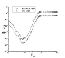
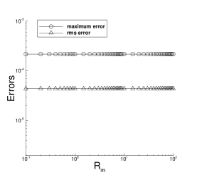
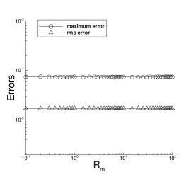
(a) (b) (c)

Figure 19: Wave equation: Maximum and rms errors of the locELM solution in the domain as a function of $R_{m}$, obtained with (a) no pre-training, (b) BIP pre-training, and (c) modBIP pre-training of the random coefficients.

Figure 19 is a further comparison of the locELM methods with no pre-training and with BIP and modBIP pre-training of the random coefficients. Plotted here are the maximum and rms errors in the overall domain of the locELM solution obtained with these three cases as a function of $R_{m}$ for generating the initial random coefficients. The local neural-network architecture and related parameters, the collocation points, and the parameters for the BIP and modBIP algorithms are the same as those for Figure 18, except that here the $R_{m}$ is varied systematically between $R_{m}=0.1$ and $R_{m}=100$ in this set of computations. Without pre-training of the initial random coefficients, one can observe a strong influence of $R_{m}$ on the locELM solution accuracy (Figure 19(a)). On the other hand, the pre-training of the random coefficients by either modBIP or BIP essentially eliminates the dependence of the solution error on $R_{m}$ (i.e. the initial random coefficients). The combined locELM/modBIP method is again observed to be more accurate than locELM/BIP.

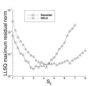
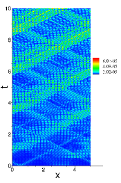
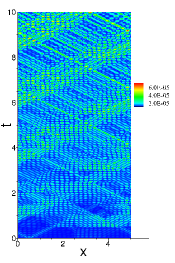
(a) (b) (c)

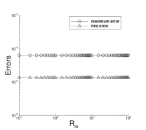
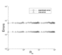
(d) (e)

Figure 20: Wave equation (non-monotonic activation functions): (a) The LLSQ maximum residual norm for estimating $S_{b}$ in modBIP, with the Gaussian and GELU HendrycksG2020 activation functions. Error distributions of the locELM/modBIP solution obtained with (b) the Gaussian, and (c) the GELU activation functions. The maximum/rms errors of the locELM/modBIP solution as a function of $R_{m}$ obtained using (d) the Gaussian, and (e) the GELU activation functions. $S_{b}=3$ in (b,d) with the Gaussian function, and $S_{b}=4$ in (c,e) with GELU, and $S_{b}$ is varied in (a). $R_{m}=50$ in (a,b,c) and is varied in (d,e).

Figure 20 demonstrates the ability of the current modBIP algorithm to work with non-invertible activation functions. By contrast, the BIP algorithm breaks down if such activation functions are present in the neural network. Specifically, this figure examines the locELM/modBIP simulation results obtained using the Gaussian function and the Gaussian error linear unit (GELU) HendrycksG2020 as the activation functions in the hidden layers of the local neural networks. Here each local neural network has an architecture $[2,250,1]$, with Gaussian or GELU as the activation function for the hidden layer, and we employ $Q=31\times 31$ uniform collocation points on each sub-domain. The initial random coefficients in the local neural networks are generated with either a fixed $R_{m}=50$ or with $R_{m}$ varied between $R_{m}=0.1$ and $R_{m}=100$, and are pre-trained using modBIP with $S_{c}=S_{b}/2$. Figure 20(a) shows the LLSQ maximum residual norms (among the $20$ time blocks) for estimating the $S_{b}$ in modBIP, which suggest a value around $S_{b}\approx 3$ with the Gaussian activation function and a value around $S_{b}\approx 4$ with the GELU activation function. Figures 20(b) and (c) show the error distributions the locELM/modBIP solution obtained using the Gaussian and GELU activation functions, respectively, with a fixed $R_{m}=50$ for generating the initial random coefficients. Figures 20(d) and (e) are the maximum and rms errors of the locELM/modBIP solution in the overall domain as a function of $R_{m}$, obtained with the Gaussian and GELU activation functions, respectively. In the plots (b)-(d), we employ $S_{b}=3$ with the Gaussian function and $S_{b}=4$ with GELU in the modBIP algorithm. It is evident that the combined locELM/modBIP produces accurate simulation results with the Gaussian and GELU activation functions, and that its errors are insensitive to the initial random coefficients.

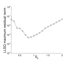
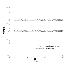
(a) (b)

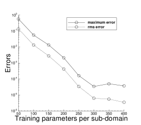
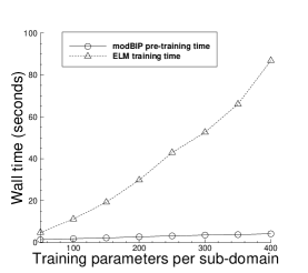
(c) (d)

Figure 21: Wave equation (3 hidden layers in neural network): (a) The LLSQ maximum residual norm for estimating the best $S_{b}$ in modBIP. The maximum and rms errors of the locELM/modBIP solution as a function of (b) $R_{m}$, and (c) the number of training parameters per sub-domain. (d) The modBIP pre-training time and the ELM network training time as a function of the number of training parameters per sub-domain. $S_{b}=0.8$ in (b,c,d), and is varied in (a). $R_{m}=50$ in (a,c,d), and is varied in (b). Local neural network architecture is $[2,50,50,M,1]$, with $M=250$ in (a,b) and varied in (c,d). $Q=31\times 31$ in (a,b,c,d).

Finally, Figure 21 is an illustration of the locELM/modBIP results with $3$ hidden layers in the local neural networks. In this group of tests, we employ an architecture $[2,50,50,M,1]$ in all the local neural networks with the $\tanh$ activation function for the hidden layers, where $M$ is either fixed at $M=250$ or varied between $M=50$ and $M=400$. We again employ $20$ uniform time blocks, $4$ uniform sub-domains within each time block, and a set of $Q=31\times 31$ uniform collocation points on each sub-domain. The initial random coefficients are generated with $R_{m}$ either fixed at $R_{m}=50$ or varied between $R_{m}=0.1$ and $R_{m}=100$. Figure 21(a) shows the LLSQ maximum residual norm for estimating $S_{b}$, suggesting a value around $S_{b}\approx 0.8$ in modBIP. Figures 21(b) and (c) show the maximum and rms errors in the overall domain of the locELM/modBIP solution as a function of $R_{m}$ and the number of training parameters per sub-domain $M$, respectively. The results signify the insensitivity of the locELM/modBIP errors with respect to the initial random coefficients, and the exponential decrease in the errors with increasing training parameters in the neural network. Figure 21(d) shows the modBIP pre-training time of the random coefficients and the ELM training time of the neural network as a function of the number of training parameters per sub-domain. While both the modBIP pre-training time and the ELM training time grows with increasing number of training parameters, the growth rate of the modBIP pre-training time is much slower than the ELM training time. For example, as the number of training parameters per sub-domain increases from $50$ to $400$, the modBIP pre-training time increases from around $1.4$ seconds to about $4.2$ seconds, while the ELM training time increases from about $4.8$ seconds to about $87$ seconds.

3.4 Diffusion Equation

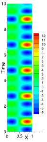
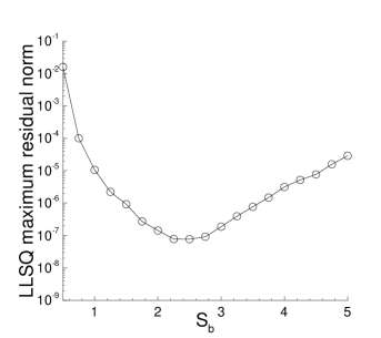
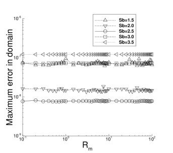
(a) (b) (c)

Figure 22: Diffusion equation: (a) Distribution of the exact solution in the spatial-temporal plane. (b) The maximum residual norm of the linear least squares (LLSQ) problem as a function of $S_{b}$, for estimating the best $S_{b}$ in modBIP. (c) The maximum error in the domain of the ELM/BIP solution as a function of $R_{m}$, corresponding to several $S_{b}$ values in modBIP. $R_{m}=100$ in (b) and is varied in (c).

As another example we test the combined ELM/modBIP method using the unsteady diffusion equation. Consider the spatial-temporal domain, $\Omega=\{\ (x,t)\ |\ x\in[0,1],\ t\in[0,10]\}$, and the following initial/boundary value problem,

$$\frac{\partial u}{\partial t}-\nu\frac{\partial^{2}u}{\partial x^{2}}=f(x,t),$$ (18a)

$$u(0,t)=g_{1}(t),$$ (18b)

$$u(1,t)=g_{2}(t),$$ (18c)

$$u(x,0)=h(x),$$ (18d)

where $u(x,t)$ is the field solution to be solved for, the constant $\nu=0.01$ denotes the diffusion coefficient, $f(x,t)$ is a prescribed source term, $g_{1}$ and $g_{2}$ are the Dirichlet boundary distributions at $x=0$ and $x=1$, and $h(x)$ is the initial distribution. We employ the following manufactured solution to this problem,

$$u(x,t)=\left[2\cos\left(\pi x+\frac{\pi}{5}\right)+\frac{3}{2}\cos\left(2\pi x-\frac{3\pi}{5}\right)\right]\left[2\cos\left(\pi t+\frac{\pi}{5}\right)+\frac{3}{2}\cos\left(2\pi t-\frac{3\pi}{5}\right)\right].$$ (19)

Accordingly, the source term $f(x,t)$, the boundary/initial distributions $g_{1}$, $g_{2}$ and $h$ are chosen such that the expression (19) satisfies the system (18). Figure 22(a) shows the distribution of the analytic solution (19) in the spatial-temporal $(x,t)$ plane.

We employ the block time-marching scheme and the combined ELM/modBIP method to solve the system (18). We divide the spatial-temporal domain $\Omega$ along the temporal direction into $10$ uniform time blocks, and solve the system (18) on each time block individually and successively (see Remark 2.7) using the combined ELM/modBIP method (see Section 2.3).

Let us first consider the neural network containing a single hidden layer, with the architecture characterized by $[2,300,1]$, the $\tanh$ activation function for the hidden layer and a linear output layer. The input layer ($2$ nodes) denotes the spatial/temporal coordinates ($x$ and $t$), and the output layer ($1$ node) represents the field solution $u(x,t)$. We employ a set of $Q=25\times 25$ uniform grid (collocation) points on each time block ($25$ points in both $x$ and $t$ directions) as the training data points, which constitute the input data into the neural network. The hidden-layer coefficients in the neural network are initialized to uniform random values generated on $[-R_{m},R_{m}]$, with $R_{m}$ either fixed at $R_{m}=100$ or varied between $R_{m}=0.1$ and $R_{m}=100$ in the subsequent tests. The initial random coefficients are pre-trained by modBIP with $S_{c}=S_{b}/2$ and $S_{b}$ determined by the procedure discussed in Remark 2.2.

Figure 22(b) shows the LLSQ maximum residual norm among the $10$ time blocks for estimating the best $S_{b}$ in modBIP, which suggests a value around $S_{b}\approx 2.5$. This set of tests are performed with a fixed $R_{m}=100$ when generating the random coefficients in the neural network. Figure 22(c) plots the maximum error in the overall domain of the ELM/modBIP solution as a function of $R_{m}$, with several $S_{b}$ values around $S_{b}=2.5$ and $S_{c}=S_{b}/2$ in the modBIP algorithm. The ELM/modBIP solution errors in this and the subsequent figures are computed as follows. After the neural network has been trained, we evaluate the neural network on a set of $101\times 101$ uniform grid points on each time block to obtain the numerical solution. The exact solution (19) is evaluated on the same set of grid points in the overall domain. Then the maximum and the rms errors of the numerical solution against the analytic solution can be computed based these data. The error of the ELM/modBIP solution can be observed to be insensitive to the initial random coefficients in the neural network, irrespective of the $S_{b}$ parameter in modBIP.

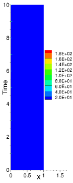
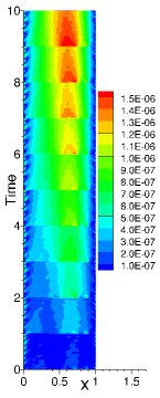
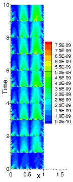
(a) (b) (c)

Figure 23: Diffusion equation: Distributions of the absolute error of the ELM solution obtained with (a) no pre-training, (b) BIP pre-training, and (c) modBIP pre-training of the random coefficients.

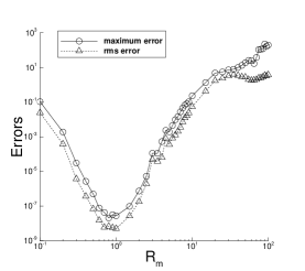
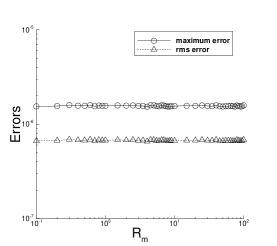
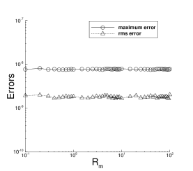
(a) (b) (c)

Figure 24: Diffusion equation: The maximum and rms errors of the ELM solution as a function of $R_{m}$ obtained with (a) no pre-training, (b) BIP pre-training, and (c) modBIP pre-training of the random coefficients.

In Figures 23 and 24 we compare the ELM method with no pre-training and with the BIP and modBIP pre-training of the random coefficients in the neural network. In the case with no pre-training, the initial random coefficients generated on $[-R_{m},R_{m}]$ are directly used in the ELM computation. In the case with BIP or modBIP pre-training, the initial random coefficients are pre-trained first, and the updated random coefficients are then used in the ELM computation. With BIP, a normal distribution for the target samples has been employed with a random mean on $[-1,1]$ and a standard deviation $0.5$ NeumannS2013 . With modBIP we employ $S_{c}=S_{b}/2$ and $S_{b}=2.5$ in the Algorithm 1. Figure 23 shows distributions in the spatial-temporal plane of the absolute error of the ELM solution obtained with no pre-training and with BIP/modBIP pre-training of the random coefficients. The initial random coefficients are generated with $R_{m}=100$ in this set of tests. The ELM solution obtained without pre-training of the random coefficients is totally off and inaccurate. On the other hand, the ELM solutions with the initial random coefficients pre-trained by BIP and modBIP are observed to be very accurate. The ELM/modBIP solution is observed to be considerably more accurate (by two or three orders of magnitude) than the ELM/BIP solution.

Figure 24 shows the maximum and rms errors of the ELM solutions, obtained with no pre-training and with BIP or modBIP pre-training of the random coefficients, as a function of $R_{m}$ for generating the initial random coefficients. The accuracy of the ELM solution without pre-training of the random coefficients strongly depends on $R_{m}$, as is evident from Figure 24(a). In contrast, with the random coefficients pre-trained by BIP or modBIP, the ELM solution accuracy becomes essentially independent of $R_{m}$ (Figures 24(b,c)). The data again signify that the ELM/modBIP solution is much more accurate than the ELM/BIP one.

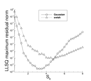
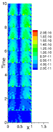
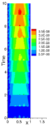
(a)  (b)  (c)

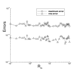
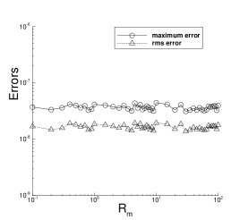
(d) (e)

Figure 25: Diffusion equation (non-monotonic activation functions): (a) The LLSQ maximum residual norm versus $S_{b}$, for estimating the best $S_{b}$ in modBIP, with the Gaussian and swish activation functions. Distributions of the absolute error of the ELM/modBIP solution obtained with (b) the Gaussian, and (c) swish activation functions. The maximum/rms errors in the domain as a function of $R_{m}$ corresponding to (d) the Gaussian, and (e) swish activation functions. $R_{m}=100$ in (a,b,c) and is varied in (d,e). $S_{b}=3$ in (b,d) for the Gaussian function, and $S_{b}=5$ in (c,e) for the swish function, and $S_{b}$ is varied in (a).

Figure 25 demonstrates the capability of the combined ELM/modBIP method to work with activation functions that do not have an inverse. Here we have considered the Gaussian and swish activation functions in the neural network. We again employ a network architecture $[2,300,1]$, with $Q=25\times 25$ uniform collocation points on each time block. The initial random coefficients are generated with $R_{m}$ fixed at $R_{m}=100$ or varied between $R_{m}=0.1$ and $R_{m}=100$. Figure 25(a) shows the LLSQ maximum residual norms for estimating the $S_{b}$ in modBIP, which suggest a value around $S_{b}\approx 3$ with the Gaussian activation function and $S_{b}\approx 5$ with the swish activation function. Figures 25(b) and (c) depict the error distributions in the spatial-temporal plane of the ELM/modBIP solution corresponding to the Gaussian activation function (with $S_{b}=3$ in modBIP) and the swish activation function (with $S_{b}=5$ in modBIP). One can observe that the combined ELM/modBIP method, especially with the Gaussian activation function, has produced very accurate results. The initial random coefficients are generated with $R_{m}=100$ in the plots (a,b,c). Figures 25(d) and (e) show the maximum/rms errors in the overall domain of the ELM/modBIP solution as a function of $R_{m}$, corresponding to the Gaussian and swish activation functions, respectively. The solution errors are not sensitive to the initial random coefficients in the neural network. It should be noted that the BIP algorithm breaks down with the type of activation functions tested here.

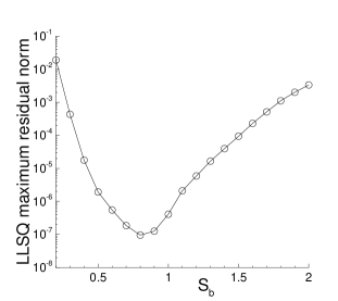
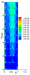
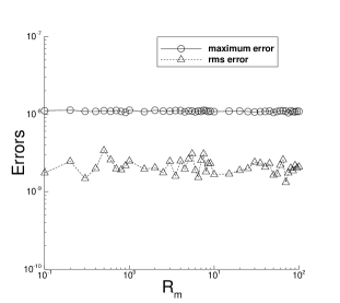
(a) (b) (c)

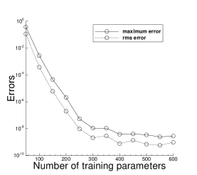
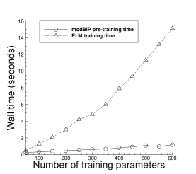
(d) (e)

Figure 26: Diffusion equation (3 hidden layers in neural network): (a) The maximum residual norm of the LLSQ problem for estimating the $S_{b}$ in modBIP. (b) Distribution of the absolute error of the ELM/modBIP solution. The maximum and rms errors in the domain as a function of (c) $R_{m}$, and (d) the number of training parameters $M$. (e) The modBIP pre-training time and the ELM network training time as a function of the number of training parameters $M$. $S_{b}=0.8$ in (b,c,d,e) and is varied in (a). $R_{m}=100$ in (a,b,d,e) and is varied in (c). $M=300$ in (a,b,c) and is varied in (d,e). $Q=25\times 25$ in (a,b,c,d,e).

Finally, Figure 26 illustrates the ELM/modBIP simulation results using multiple hidden layers in the neural network. Here $10$ uniform time blocks are used in the domain for block time marching. The neural network architecture is characterized by $[2,50,50,M,1]$, where the number of training parameters $M$ is fixed at $M=300$ or varied between $M=50$ and $M=600$. The $\tanh$ activation function is used for all the hidden layers. We employ $Q=Q_{1}\times Q_{1}$ uniform collocation points within each time block, where $Q_{1}$ is either fixed at $Q_{1}=25$ or varied between $Q_{1}=5$ and $Q_{1}=50$. The initial random coefficients are generated with a fixed $R_{m}=100$ or with $R_{m}$ varied between $R_{m}=0.1$ and $R_{m}=100$. These random coefficients are pre-trained by modBIP with $S_{c}=S_{b}/2$ and $S_{b}$ estimated by the procedure in Remark 2.2. The specific parameter values for each plot are provided in the caption of the figure. Figure 26(a) shows the LLSQ residual norms versus $S_{b}$ for estimating the best $S_{b}$ in modBIP, which suggests a value around $S_{b}\approx 0.8$ in the algorithm. Figure 26(b) illustrates the error distribution of the ELM/modBIP solution in the spatial-temporal plane, demonstrating that the method produces accurate simulation results. Figure 26(c) depicts the maximum and rms errors in the overall domain of the ELM/modBIP solution as a function of $R_{m}$ for generating the initial random coefficients, indicating that the accuracy of the ELM/modBIP method is not sensitive to the initial random coefficients with multiple hidden layers in the neural network. Figure 26(d) shows the maximum/rms errors of the ELM/modBIP solution as a function of the number of training parameters ($M$), indicating an exponential decrease in the errors (before saturation) with this method. Figure 26(e) shows the modBIP pre-training time and the ELM network training time as a function of the number of training parameters in the neural network. The modBIP pre-training time grows very slowly as the number of training parameters increases. Its growth rate is much smaller compared with that of the ELM training time.

4 Concluding Remarks

We have presented an effective algorithm (termed modBIP) for pre-training the random hidden-layer coefficients of extreme learning machines (ELM), and applied the combined ELM/modBIP method to function approximations and solving partial differential equations. The initial random coefficients in the neural network are first pre-trained by modBIP, and the updated hidden-layer coefficients are then fixed and employed in the least squares computation with the ELM method. The modBIP algorithm is devised based on the same principle as the batch intrinsic plasticity (BIP) method, namely, by enhancing the information transmission in every node of the neural network.

Suppose the neural network architecture is chosen, which may be shallow or deep, the hidden-layer coefficients are initialized to random values, and that the input data to the neural network are given. The modBIP algorithm pre-trains the random hidden-layer coefficients as follows. For each node in each hidden layer of the neural network, this algorithm first computes the total (synaptic) input to this node for all input data samples to the neural network. The synaptic input samples are then mapped, by an affine mapping, to a set of random target samples on a random sub-interval of $[-S_{b},S_{b}]$ with a minimum size, where $S_{b}$ is a user-provided hyper-parameter. The coefficients in the affine mapping are determined by solving a linear least squares problem, and are used to update the random weight and bias coefficients associated with this node. These operations are performed on each hidden layer, individually and successively, and within each hidden layer node by node. For a given particular problem, the $S_{b}$ parameter in modBIP can be estimated with preliminary simulations by computing the residual norm of the least squares problem associated with the least squares solution in ELM; see the procedure outlined in Remark 2.2.

The modBIP method differs from BIP NeumannS2013 in one prominent aspect: modBIP does not involve the activation function in its algorithm. In contrast, the BIP method employs the inverse of the activation function in its construction, and requires the activation function to be invertible (or monotonic). This limits the applicability of BIP to neural networks with only monotonic activation functions. On the other hand, the modBIP method can be applied with essentially any activation function, including those often-used non-monotonic activation functions such as the Gaussian function, swish function, Gaussian error linear unit (GELU), and the class of radial basis activation functions.

Another crucial construction in modBIP is the random sub-interval of $[-S_{b},S_{b}]$ with a minimum size $S_{c}$, on which the random target samples are generated. This is the key that accounts for the high accuracy of the modBIP (combined with ELM) results. If this sub-interval is fixed, instead of being random, much of the high accuracy will be lost. As demonstrated by ample numerical experiments, when combined with ELM, the modBIP method typically produces much more accurate simulation results than BIP.

In the current paper we have used partial differential equations to test the combined ELM/modBIP method, and presented extensive numerical experiments to evaluate its computational performance. We have the following observations:

• The combined ELM/modBIP method produces highly accurate simulation results, and its accuracy is insensitive to the initial random coefficients of the neural network. More precisely, its accuracy is insensitive to the $R_{m}$ for generating the initial random coefficients. In contrast, without pre-training the random coefficients, the accuracy of the ELM solution is strongly dependent on $R_{m}$, where the initial random coefficients are generated on $[-R_{m},R_{m}]$.

• The combined ELM/modBIP method works well with non-monotonic activation functions, and produces highly accurate results. With the Gaussian activation function, the combined ELM/modBIP method appears to produce generally the most accurate results among the activation functions tested herein. In contrast, the BIP method NeumannS2013 breaks down with non-monotonic activation functions.

• Irrespective of the initial random coefficients, the errors of the combined ELM/modBIP solution decrease exponentially or nearly exponentially, as the number of training data points in the domain or the number of training parameters in the neural network increases.

• The combined ELM/modBIP method works well with both shallow and deep neural networks. The favorable numerical properties, such as the error insensitivity to initial random coefficients and the exponential convergence with respect to the collocation points and the training parameters, are observed with both shallow and deep neural networks.

• The computational cost of the modBIP pre-training of the random coefficients is low, and it is only a fraction of the ELM training cost of the neural network. In typical simulations the modBIP pre-training cost is within $10\%$ of the ELM training cost for the neural network. Furthermore, the modBIP pre-training of the random coefficients logically only needs to be performed once for a given network architecture and the input data, and the pre-trained random coefficients can be saved and used later directly by ELM.

The numerical results demonstrate unequivocally that modBIP provides an efficient and effective technique for pre-training the random coefficients to achieve high accuracy with ELM. It significantly boosts the computational performance of ELM. The combined ELM/modBIP method can produce accurate simulation results, regardless of the initial random coefficients in the neural network. This method is promising in terms of both the accuracy and the computational cost. We anticipate that the ELM/modBIP method will be useful to and instrumental in neural network-based scientific computing and the computational understanding of important physical processes and phenomena Dong2018 ; Dong2014obc .

References

- [1] W. Cao, L. Hu, J. Gao, X. Wang, and Z. Ming. A study on the relationship between the rank of input data and the performance of random weight neural network. Neural Computing and Applications, 32:12685–12696, 2020.
- [2] S. Dong. An outflow boundary condition and algorithm for incompressible two-phase flows with phase field approach. Journal of Computational Physics, 266:47–73, 2014.
- [3] S. Dong. A convective-like energy-stable open boundary condition for simulations of incompressible flows. Journal of Computational Physics, 302:300–328, 2015.
- [4] S. Dong. Wall-bounded multiphase flows of N immiscible incompressible fluids: consistency and contact-angle boundary condition. Journal of Computational Physics, 338:21–67, 2017.
- [5] S. Dong. Multiphase flows of N immiscible incompressible fluids: a reduction-consistent and thermodynamically-consistent formulation and associated algorithm. Journal of Computational Physics, 361:1–49, 2018.
- [6] S. Dong and Z. Li. Local extreme learning machines and domain decomposition for solving linear and nonlinear partial differential equations. arXiv:2012.02895, 2020.
- [7] S. Dong and N. Ni. A method for representing periodic functions and enforcing exactly periodic boundary conditions with deep neural networks. Journal of Computational Physics, 435:110242, 2021.
- [8] S. Dong and J. Shen. A pressure correction scheme for generalized form of energy-stable open boundary conditions for incompressible flows. Journal of Computational Physics, 291:254–278, 2015.
- [9] G. Dudek. Generating random weights and biases in feedforward neural networks with random hidden nodes. Information Sciences, 481:33–56, 2019.
- [10] V. Dwivedi and B. Srinivasan. Physics informed extreme learning machine (pielm) a rapid method for the numerical solution of partial differential equations. Neurocomputing, 391:96–118, 2020.
- [11] W. E and B. Yu. The deep Ritz method: a deep learning-based numerical algorithm for solving variational problems. Communications in Mathematics and Statistics, 6:1–12, 2018.
- [12] S. Elfwing, E. Uchibe, and K. Doya. Sigmoid-weighted linear units for neural network function approximation in reinforcement learning. Neural Networks, 107:3–11, 2018.
- [13] A.L. Freire, A.R. Rocha-Neto, and G.A. Barreto. On robust randomized neural networks for regression: a comprehensive review and evaluation. Neural Computing and Applications, 32:16931–16950, 2020.
- [14] G.H. Golub and C.F.V. Loan. Matrix Computations, 3rd Ed. Johns Hopkins Press, MD, 1996.
- [15] I. Goodfellow, Y. Bengio, and A. Courville. Deep Learning. The MIT Press, 2016.
- [16] S. Haykin. Neural Networks: A Comprehensive Foundation. Prentice Hall, 1999.
- [17] J. He and J. Xu. MgNet: A unified framework for multigrid and convolutional neural network. Science China Mathematics, 62:1331–1354, 2019.
- [18] D. Hendrycks and K. Gimpel. Gaussian error linear units (GELU). arXiv:1606.08415, 2016.
- [19] G. Huang, G.B. Huang, S. Song, and K. You. Trends in extreme learning machines: a review. Neural Networks, 61:32–48, 2015.
- [20] G.-B. Huang, Q.-Y. Zhu, and C.-K. Siew. Extreme learning machine: theory and applications. Neurocomputing, 70:489–501, 2006.
- [21] B. Igelnik and Y.H. Pao. Stochastic choice of basis functions in adaptive function approximation and the functional-link net. IEEE Transactions on Neural Networks, 6:1320–1329, 1995.
- [22] H. Jaeger, M. Lukosevicius, D. Popovici, and U. Siewert. Optimization and applications of echo state networks with leaky integrator neurons. Neural Networks, 20:335–352, 2007.
- [23] A.D. Jagtap, E. Kharazmi, and G.E. Karniadakis. Conservative physics-informed neural networks on discrete domains for conservation laws: applications to forward and inverse problems. Computer Methods in Applied Mechanics and Engineering, 365:113028, 2020.
- [24] I.E. Lagaris, A.C. Likas, and D.I. Fotiadis. Artificial neural networks for solving ordinary and partial differential equations. IEEE Transactions on Neural Networks, 9:987–1000, 1998.
- [25] J.-Y. Li, W. Chow, B. Igelnik, and Y.-H. Pao. Comments on “stochastic choice of basis functions in adaptive function approximaton and the functional-link net”. IEEE Trans. Neural Netw., 8:452–454, 1997.
- [26] L. Lu, P. Jin, and G.E. Karniadakis. DeepONet: learning nonlinear operators for identifying differential equations based on the universal approximation theorem of operators. arXiv:1910.03193, 2019.
- [27] M. Lukosevicius and H. Kaeger. Reservoir computing approaches to recurrent neural network training. Comput. Sci. Rev., 3:127–149, 2009.
- [28] W. Maas and H. Markram. On the computational power of recurrent circuits of spiking neurons. J. Comput. Syst. Sci., 69:593–616, 2004.
- [29] M.D. McDonnell, M.D. Tissera, T. Vladusich, A. van Schaik, and J. Tapson. Fast, simple and accurate handwritten digit classification by training shallow neural network classifiers with the extreme learning algorithm. PLoS ONE, 10(8):e0134254, 2015.
- [30] K. Neumann and J.J. Steil. Optimizing extreme learning machines via ridge regression and batch intrinsic plasticity. Neurocomputing, 102:23–30, 2013.
- [31] S. Panghal and M. Kumar. Optimization free neural network approach for solving ordinary and partial differential equations. Engineering with Computers, Early Access, February 2020.
- [32] Y.H. Pao, G.H. Park, and D.J. Sobajic. Learning and generalization characteristics of the random vector functional-link net. Neurocomputing, 6:163–180, 1994.
- [33] M. Raissi, P. Perdikaris, and G.E. Karniadakis. Physics-informed neural networks: a deep learning framework for solving forward and inverse problems involving nonlinear partial differential equations. Journal of Computational Physics, 378:686–707, 2019.
- [34] F. Rosenblatt. The perceptron: a probabilistic model for information storage and organization in the brain. Psychol. Rev., 65:386–408, 1958.
- [35] K. Rudd and S. Ferrari. A constrained integration (CINT) approach to solving partial differential equations using artificial neural networks. Neurocomputing, 155:277–285, 2015.
- [36] E. Samanaiego, C. Anitescu, S. Goswami, V.M. Nguyen-Thanh, H. Guo, K. Hamdia, X. Zhuang, and T. Rabczuk. An energy approach to the solution of partial differential equations in computational mechanics via machine learning: concepts, implementation and applications. Computer Methods in Applied Mechanics and Engineering, 362:112790, 2020.
- [37] S. Scardapane and D. Wang. Randomness in neural networks: an overview. WIREs Data Mining Knowl. Discov., 7:e1200, 2017.
- [38] J. Sirignano and K. Spoliopoulos. DGM: A deep learning algorithm for solving partial differential equations. Journal of Computational Physics, 375:1339–1364, 2018.
- [39] J.J. Steil. Online reservoir adaption by intrinsic plasticity for backpropagation decorrelation and echo state learning. Neural Networks, Special Issue on Echo State and Liquid State Networks, pages 353–364, 2007.
- [40] J. Triesch. A gradient rule for the plasticity of a neuron’s intrinsic excitability. Proceedings of the ICANN, pages 65–79, 2005.
- [41] D. Wang and M. Li. Stochastic configuration networks: fundamentals and algorithms. IEEE Transactions on Cybernetics, 47:3466–3479, 2017.
- [42] Y. Wang and G. Lin. Efficient deep learning techniques for multiphase flow simulation in heterogeneous porous media. Journal of Computational Physics, 401:108968, 2020.
- [43] C.S. Webster. Alan Turing’s unorganized machines and artificial neural networks: his remarkable early work and future possibilities. Evol. Intel., 5:35–43, 2012.
- [44] P.J. Werbos. Beyond regression: new tools for prediction and alaysis in the behavioral sciences. PhD Thesis, Harvard Univeristy, Cambridge, MA, 1974.
- [45] B. Widrow, A. Greenblatt, Y. Kim, and D. Park. The no-prop algorithm: a new learning algorithm for multilayer neural networks. Neural Networks, 37:182–188, 2013.
- [46] N. Winovich, K. Ramani, and G. Lin. ConvPDE-UQ: Convolutional neural networks with quantified uncertainty for heterogeneous elliptic partial differential equations on varied domains. Journal of Computational Physics, 394:263–279, 2019.
- [47] W. Xing, R.M. Kirby, and S. Zhe. Deep corgionalization for the emulation of spatial-temporal fields. arXiv:1910.07577, 2019.
- [48] J. Xu. The finite neuron method and convergence analysis. arXiv:2010.01458, 2020.
- [49] Y. Yang and Q.M.J. Wu. Extreme learning machine with subnetwork hidden nodes for regression and classification. IEEE Transactions on Cybernetics, 46:2885–2898, 2016.
- [50] Y. Zang, G. Bao, X. Ye, and H. Zhou. Weak adversarial networks for high-dimensional partial differential equations. Journal of Computational Physics, 411:109409, 2020.