Testing for the Network Small-World Property

Abstract

Researchers have long observed that the “small-world” property, which combines the concepts of high transitivity or clustering with a low average path length, is ubiquitous for networks obtained from a variety of disciplines including social sciences, biology, neuroscience, and ecology. However, we find three shortcomings of the currently popular definition and detection methods rendering the concept less powerful. First, the classical definition combines high transitivity with a low average path length in a rather ad-hoc fashion which confounds the two separate aspects. We find that in several cases, networks get flagged as “small world” by the current methodology solely because of their high transitivity. Second, the detection methods lack a formal statistical inference, and third, the comparison is typically performed against simplistic random graph models as the baseline which ignores well-known network characteristics. We propose three innovations to address these issues. First, we decouple the properties of high transitivity and low average path length as separate events to test for. Second, we define the property as a statistical test between a suitable null model and a superimposed alternative model. Third, the test is performed using parametric bootstrap with several null models to allow a wide range of background structures in the network. In addition to the bootstrap tests, we also propose an asymptotic test under the Erdös-Renýi null model for which we provide theoretical guarantees on the asymptotic level and power. Applying the proposed methods on a large number of network datasets, we uncover new insights about their small-world property.

1 introduction

The “small-world property” is one of the most widely observed properties of complex networks encountered in applications across a range of disciplines (Watts and Strogatz, 1998; Amaral et al., 2000; Humphries and Gurney, 2008; Bassett and Bullmore, 2006). The idea of a “small-world” in networks was first conceived and experimentally validated in the context of social networks by Milgram, (1967) and was formulated in its currently used form in the seminal work by Watts and Strogatz, (1998). Roughly, the small-world property consists of “segregation” of vertices into small tightly knit groups that leads to high local clustering in an otherwise sparse network, while at the same time the network has a small average path length that “integrates” the network. Over the last two decades, “small-world” networks have been observed in anatomical and functional brain networks (Bassett and Bullmore, 2006; He et al., 2007; Bullmore and Sporns, 2009; Sporns, 2014; Rubinov and Sporns, 2010; Bassett and Bullmore, 2017), metabolic networks (Jeong et al., 2000; Wagner and Fell, 2001), protein-protein interaction networks (Jeong et al., 2001; Wagner, 2001), gene co-expression network (Van Noort et al., 2004), the internet (Albert and Barabási, 2002), ecological networks and food webs Montoya and Solé, (2002); Williams et al., (2002); Sole and Montoya, (2001), scientific collaboration networks Newman, (2001), and air transportation networks Guimera et al., (2005). Some authors have also wondered if the small-world property is “ubiquitous” (Telesford et al., 2011) or even “nearly-universal” for networks Bassett and Bullmore, (2017), while some have questioned the usefulness of the measure if it indeed is a universal property Bassett and Bullmore, (2017).

The small-worldness of networks is particularly well studied in the context of brain networks obtained from both structural and functional neuroimaging studies (Bassett and Bullmore, 2006; He et al., 2007; Bullmore and Sporns, 2009; Sporns, 2014; Humphries et al., 2005; Bassett and Bullmore, 2017). It has been theorized that small-world topology reduces wiring costs and makes networks more efficient. The property has also been contrasted and implicated in several neurophysiological disorders and conditions including Schizophrenia and Alzheimer (Lynall et al., 2010; Liu et al., 2008).

The term “small-world” is traditionally used to mean the average distance between pairs of vertices, $L$, is small and similar to that of a random graph (i.e., $O(\log n)$ or less as $n$ increases). Therefore, even for large networks, the average number of hops needed to reach one vertex from another is quite small. The authors in Watts and Strogatz, (1998) showed that a large number of real-life networks have small $L$ (comparable to a random graph) but at the same time high global clustering coefficient $C$ (comparable to a regular lattice). In the modern use of the term small world, the term refers to both of these properties simultaneously holding.

The commonly accepted definition of the small-world coefficient is $\sigma=\frac{\hat{C}/C_{R}}{\hat{L}/L_{R}}$, where $\hat{C}$ and $\hat{L}$ are observed global clustering coefficient and average path length respectively, while $C_{R}$ and $L_{R}$ are the expected values of the same quantities in a Erdös-Renýi random graph (ER) of equivalent density (Watts and Strogatz, 1998; Humphries et al., 2005; Humphries and Gurney, 2008; Bassett et al., 2008; Bullmore and Sporns, 2009; Guye et al., 2010).

Shortcomings of small world property measure and methods

Despite almost four decades of empirical and methodological work on the property, several aspects of the measure and the methods popularly used to detect small-world property have been criticized in the literature Papo et al., (2016); Bialonski et al., (2010); Hlinka et al., (2017); Ansmann and Lehnertz, (2011); Muldoon et al., (2016). For example, it is rather surprising that little work exists on the quantification of uncertainty and statistical significance of the measure. The small-world coefficient can be thought of as measuring the ratio of $C/L$ between the observed network against what one would expect from an Erdös-Renýi baseline model. However, the methods lack the statistical theory of a formal test and usually do not come with a p-value to quantify the significance of the ratio. Therefore, it is not clear that what value of the coefficient should be considered high enough to call a network small world Telesford et al., (2011); Hilgetag and Goulas, (2016).

The coefficient further suffers from an issue of linear scaling, whereby larger networks are more likely to have a higher small-world coefficient than smaller networks purely due to their size Humphries and Gurney, (2008); Telesford et al., (2011). In addition, we find in our analysis in this paper that the small world measure is heavily influenced by the clustering coefficient, and in most cases using this measure leads to the same decision as just using the clustering coefficient.

In an attempt to remedy the shortcomings of the coefficient, two alternative formulations of the small world coefficient have also been considered in the literature that compares $\hat{L}$ with $L$ expected from a random graph and $\hat{C}$ with $C$ obtained from (deterministic) ring lattice Telesford et al., (2011); Muldoon et al., (2016). However, neither approach include a test of statistical significance of observed values of the coefficients.

Moreover, both the classical procedure and the modifications proposed in the literature ignore the presence of community structure and presence of hub structure due to degree heterogeneity, both of which are capable of generating networks with substantial small-world properties. It has been shown that highly modular networks are segregated and tends to produce a high clustering coefficient Pan and Sinha, (2009); Meunier et al., (2010), while networks with high degree hub nodes facilitate communication between modules leading to a short average path length. However, highly modular networks usually do not have small path lengths and the addition of random edges to decrease the path length destroys the modular organization Gallos et al., (2012). Hence it seems relevant to understand if the small-world property is a manifestation beyond the simultaneous presence of community and hub structure. After accounting for such structures, perhaps the near universality will give away to the specialty of highly small-world networks, making the small-world property more “useful”. Finally, the alternative model is rarely fully specified and consequently, the statistical powers of such procedures are unknown.

Our contributions

In view of these serious limitations of the classical definition of small-world coefficient and the procedure of estimating it, we propose a different strategy. Our contributions are as follows.

1. We replace the concept of small world coefficient with an intersection criteria as a mechanism for determining if a network is small world network. The intersection criteria decouples high clustering coefficient and low average path length into two separate criteria that can be tested separately. We implement the intersection test as a combination of two tests whose simultaneous rejection determines if an observed network is significantly more small world than a posed null model. We find that in many real world networks the decisions based on the small world coefficient is driven almost entirely by high clustering coefficient and changes in the average path length has minimal effect similar to the observation in Telesford et al., (2011). We also observe, similar to Gallos et al., (2012), that modular networks tend to have higher average path length despite being classified as small world using the small-world coefficient.

2. We propose to use a number of different random graph models as null models and define a class of alternative superimposed small world models. The expansion of null models include the Chung-Lu random graph model, the stochastic block model and the degree corrected stochastic block model. Together these models explain a variety of observed network characteristics including degree heterogeneity, modular organization, and hub structure.

3. We develop an asymptotic test with Erdös-Renýi random graph being the null model and theoretically study the asymptotic level and power of the resulting test. This is the first detection method for small world property that does not require comparison with simulated networks from a benchmark model and hence is computationally efficient for large networks. As a byproduct of our analysis we also derive that the clustering coefficient in Erdös-Renýi random graph approximately follows a lognormal distribution.

   A key shortcoming of the existing small-world toolbox is that networks are compared with the simple Erdös-Renýi random graph. It is well-known that, in contrast to the Erdös-Renýi model, real-world networks exhibit a range of properties such as degree heterogeneity, transitivity, preferential attachment, and community structure (Aiello et al., 2000; Hoff et al., 2002; Vázquez, 2003; Bickel and Chen, 2009; Fortunato, 2010; Sengupta and Chen, 2015, 2018). Crucially, a network with such properties can masquerade as a small-world network when compared to the Erdös-Renýi model. For example, a network with community structure or transitivity is likely to exhibit significantly higher clustering than Erdös-Renýi graphs. To address this shortcoming, we need to test networks against more general null models which account for such properties.

   For more general null models, we further develop a bootstrap test. Our bootstrap detection method involves computing a p-value for the statistical significance of the observed deviation of $C$ and $L$ from a suitable random graph model denoting the null hypothesis. For four different null network models described previously, we derive procedures to compute p-values of the test statistic using parametric bootstrap. This approach has two advantages over the usual (single value) small world coefficient. First, the p-value indicates the strength of the observed small-world coefficient and in particular how rare it is to observe such a high value from the null model. Second, with the choice of the null model being flexible we can determine whether an observed network is small-world controlling for other topological properties of the network of interest.

2 The null and the alternative hypotheses and superimposed Newman-Watts type models

To formalize the notion of small-worldness in terms of a statistical hypothesis on a parameter, we consider the Newman-Watts small-world model (Newman and Watts, 1999). The Newman-Watts model is a modification of the original Watts-Strogatz model of Watts and Strogatz, (1998), and is also based on an interpolation between (or mixture of) a regular ring lattice and an Erdös-Renýi random graph. The Newman-Watts model fixes problems in the Watts-Strogatz model related to having a finite probability of the lattice becoming detached and non-uniformity of the distribution of the shortcuts, and makes the model suitable for an anlytic treatment (Newman and Watts, 1999). The particular variation of the model that we consider in this paper is parameterized by three quantities — the number of vertices $n$, the expected degree $2\delta$, and the mixing proportion $\beta\in[0,1]$. A network from this model is generated as follows:

1. Construct a $\left\lceil{2\delta\beta}\right\rceil$-regular ring lattice of $n$ nodes, where $\lceil\cdot\rceil$ denotes the ceiling function. To do this, first construct a cycle of $n$ nodes, which is a 2-regular ring lattice. Then, connect each node to its neighbors that are two hops away, thereby forming a 4-regular ring lattice, and continue until $\left\lceil{\delta\beta}\right\rceil$ hops.

2. Next, for each of the ${n\choose 2}$ node pairs, randomly add an edge connecting them with probability $p=\frac{2\delta-\left\lceil{2\delta\beta}\right\rceil}{n-1}$.

We assume $\delta\rightarrow\infty$, as $n\rightarrow\infty$ and $\beta$ is a constant not dependent on $n$. Clearly for $\beta=1$, the random graph portion of the mixture is an empty graph and this model yields a $\left\lceil{2\delta}\right\rceil$ regular ring lattice with high global clustering coefficient and high average path length. On the other hand, for $\beta=0$, the ring lattice portion of the mixture is an empty graph, and this model yields a pure Erdös-Renýi random graph with $n$ nodes and $p=\frac{2\delta}{n-1}$. For $0<\beta<1$, this model yields small-world networks with high global clustering coefficient and low average path length.

The model can be viewed as a mixture or superimposed model similar to the superimposed stochastic block model in Paul et al., (2018). We note that the model will produce some multi-edges, however, the number of such multi-edges is small compared to total number of edges. Also, when considering higher order structures, e.g., connected triples or triangles, which are required to define small-world property, the edges from the two components of the mixture will interact with each other to produce certain “incidental” higher order structures in addition to model component generated structures Paul et al., (2018); Chandrasekhar and Jackson, (2016).

Under this model, we define the detection of small world property as the test of the hypothesis

$$H_{0}:\beta\in\{0,1\}\text{ vs }H_{1}:0<\beta<1.$$

The null hypothesis asserts that the network is either a pure ER random graph with parameters $(n,\frac{2\delta}{n-1})$ or a pure ring lattice, while the alternative model denoted as NW-ER$(n,2\delta,\beta)$ implies the presence of significant small-world property. Rejection of the null hypothesis is equivalent to designating a network as small world.

Extension to SBM, CL and DCSBM null models

The above superimposed alternative model framework can be extended to include other null models we might be interested in. We consider three such models, namely the Degree Corrected Stochastic Block Model (DCSBM), the Stochastic Blockmodel (SBM), and the Chung-Lu (CL) model.

The SBM exhibits community structure, the CL model exhibits preferential attachment, and the DCSBM exhibits both preferential attachment and community structure. Therefore, by using the DCSBM as the null model, we can test whether a network has small-world property after accounting for both properties. Similarly, by using the SBM as the null model, we can test for small-world property after accounting for community structure only, and by using the CL model as the null model, we can test for small-world property after accounting for preferential attachment only,

Let us consider the case of Degree Corrected Stochastic Block Model (DCSBM) since the other two are special cases of this model.

The alternative model can be described as follows:

1. Fix, the following quantities. (a) The number of communities $k$ and $n$ dimensional community assignment vector $z$. (b) The $n$ dimensional vector of degree parameters $\theta$, such that $\sum_{i:z_{i}=q}\theta_{i}=1$, (c) a $k\times k$ matrix of parameters $B$ such that $\sum_{q,l}B_{ql}=1.$ (d) A constant $0\leq\beta\leq 1$.

2. Construct a $\left\lceil{2\delta\beta}\right\rceil$-regular ring lattice of $n$ nodes as before.

3. Next, for each of the ${n\choose 2}$ node pairs, add an edge connecting them according to the outcome of the Bernoulli trial

   $$A_{ij}\sim Bernoulli(n(2\delta-\left\lceil{2\delta\beta}\right\rceil)\theta_{i}\theta_{j}B_{z_{i}z_{j}}).$$

Note $\theta,z,B$ are not dependent on $\beta$. Essentially, for this alternative model, as we decrease the value of $\beta$ away from 1, three key properties of the DCSBM null model, namely, average density, degree heterogeneity and community memberships are approximately being preserved. The only quantity that changes with $\beta$ is how much information is available regarding the DCSBM portion of the model. Again, for $\beta=0$, the DCSBM portion of the mixture yields an empty graph and this model yields a $2\delta$ regular ring lattice, while for $\beta=1$, the ring lattice is an empty graph, and this model yields a graph from DCSBM model.

The hypothesis we will test is as before,

$$H_{0}:\beta=\{0,1\}\text{ vs }H_{1}:0<\beta<1.$$

3 The intersection criteria and testing procedure

Define $E_{ij},V_{ijk},T_{ijk}$ as random variables denoting the number of edges between node pair $i,j$, the number of open triples or $V$ structures (2 of the 3 possible edges exist and the third one does not exist) among the node triple $i,j,k$, and the number of closed triples or triangle structures among the node triple $i,j,k$ respectively. Let $S_{ijk}=3T_{i,j,k}+V_{i,j,k}$ denotes the number of connected triples (i.e., sum of open and closed triple structures) among $i,j,k$. Further let $E,V,T,S$ denote the total number of edges, open triples, triangles, and connected triples in the graph. As previously defined $C=\frac{3T}{3T+V}$ is the clustering coefficient or transitivity of the graph and $L$ is the average (shortest) path length of the graph.

The test statistic

We propose a multiple testing procedure with two test statistics $[C,L]$, which we call the intersection test. In particular we reject the null hypothesis if,

$$\{C>K_{1}\}\cap\{L<K_{2}\},$$ (3.1)

for suitable choices of $K_{1}$ and $K_{2}$. The quantities $K_{1}$ and $K_{2}$ are either high quantiles of the null hypothesis sampling distribution or quantities which are “high” in comparison to the null hypothesis sampling distribution.

To provide an intuition for the test consider the case when the null model is the ER model. When the network is generated from the ER model, the first event is low-probability, the second event is high-probability, which means the intersection event is low-probability and therefore we fail to reject. On the other hand, when the the network is generated from the Newman-Watts model with mixing parameter $\beta$, the first event is high-probability (since clustering is greater), the second event is high-probability (distances are still small), which means the intersection event is high-probability and therefore we reject. However, When the the network is generated from a pure lattice, the first event is high-probability (since clustering is greater), the second event is low-probability (distances are much higher than ER), which means the intersection event is low-probability and therefore we fail to reject. Thus the intersection test ensures we have the correct decision under all three scenarios (Table 1).

Network Model	SW	$C>K_{1}$	$L<K_{2}$	Intersection Test
Pure Erdös-Renýi ($\beta=0$)	No	No	Yes	Not rejected
Newman-Watts ($0<\beta<1$)	Yes	Yes	Yes	Rejected
Pure Ring Lattice ($\beta=1$)	No	Yes	No	Not rejected

Table 1: Heuristics of the Intersection Test

Bootstrap test

We determine the cutoffs through a parametric bootstrap procedure which involves fitting the respective null model to the observed data to estimate the parameters of the null model. An adequate number ($B$) of graphs are sampled from the fitted null distribution parameters. We define a test with 6% nominal level (i.e., probability of Type I error is less than or equal to 6%) by letting $K_{1}$ be the 95th percentile of the distribution of $C$ and $K_{2}$ to be the 99th percentile of the distribution of $L$. For fitting SBM and DCSBM to the observed networks, we first estimate the number of communities $k$ using the Louvain method Blondel et al., (2008). We then estimate the community assignments with a spectral clustering procedure that involves the following steps: (i) eigendecomposition of the adjacency matrix and creation of the matrix of $k$ eigenvectors $U_{n\times k}$ that correspond to the $k$ largest eigenvalues in absolute value, (ii) projection of rows of $U$ to the unit circle and (iii) k-means clustering of the rows of the matrix $U$. Finally the model parameters are estimated using method of moments. The spectral clustering method is known to be consistent for the problem of estimating community structure from SBM and DCSBM when the number of communities are known Rohe et al., (2011); Gao et al., (2017); Lei and Rinaldo, (2015); Chin et al., (2015).

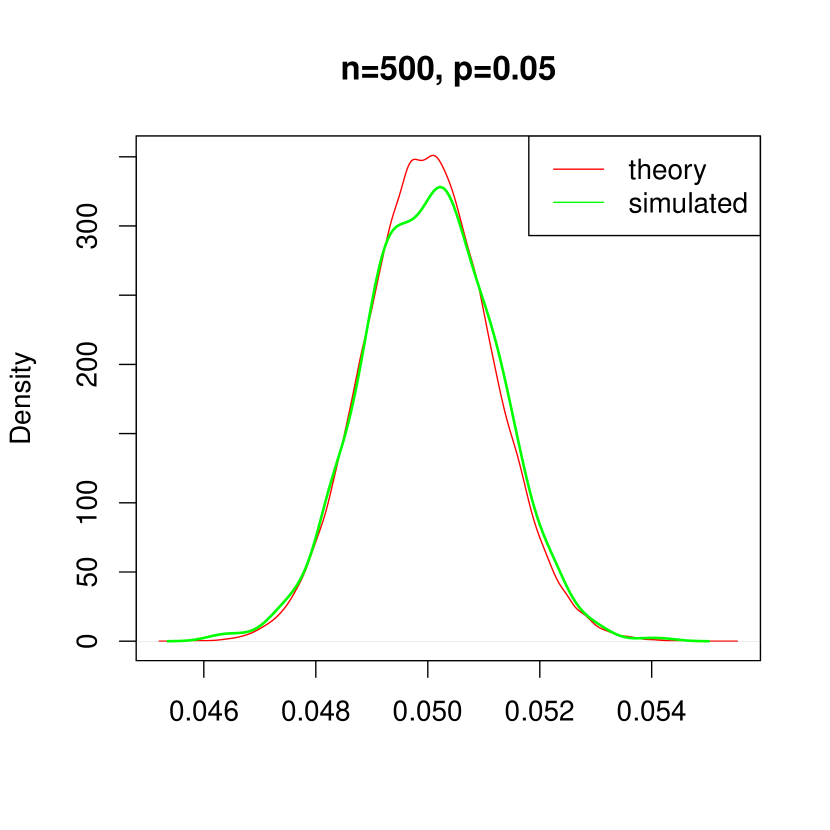
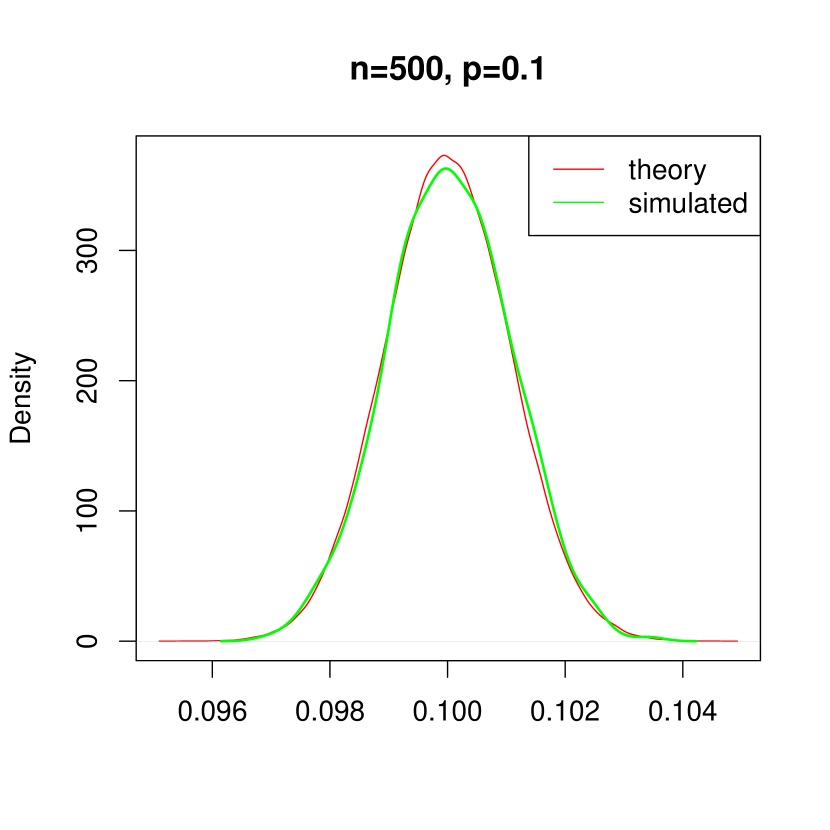
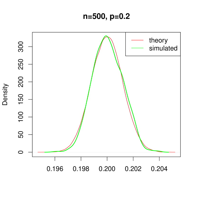
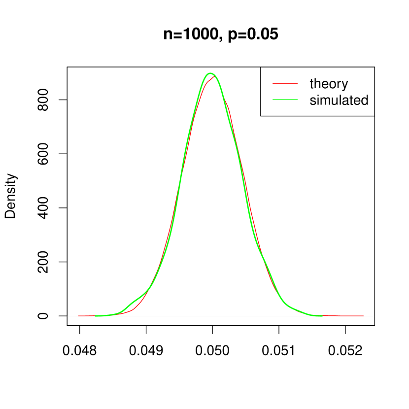
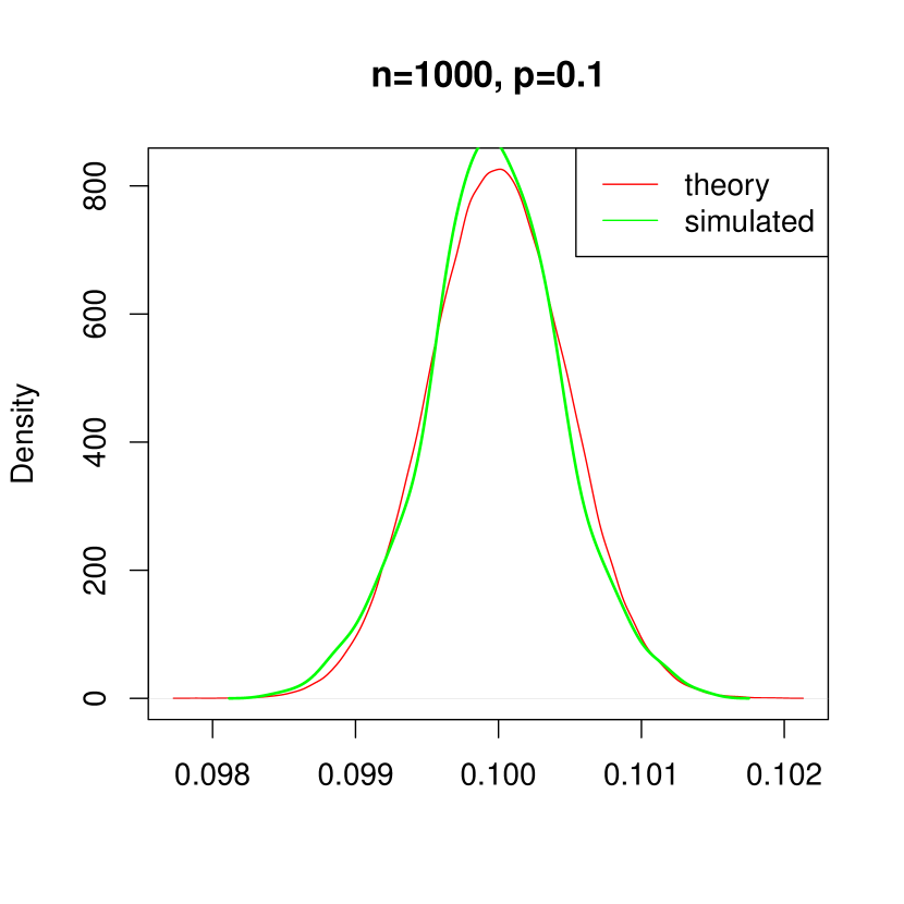
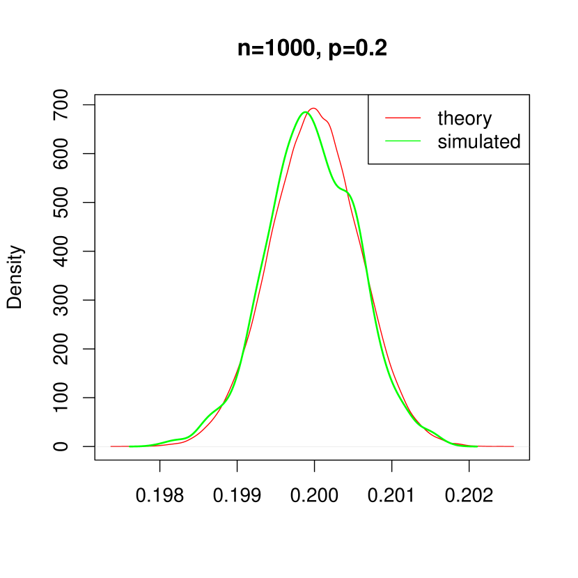
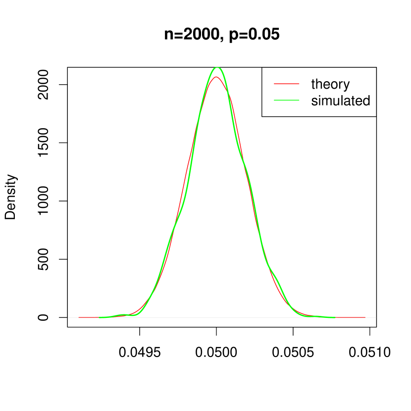
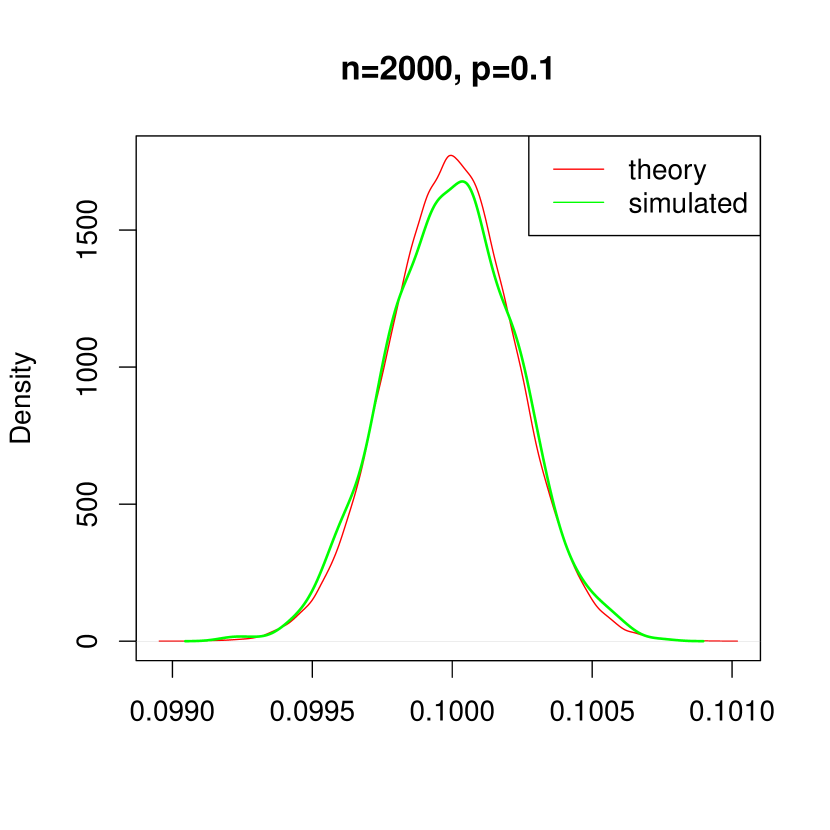
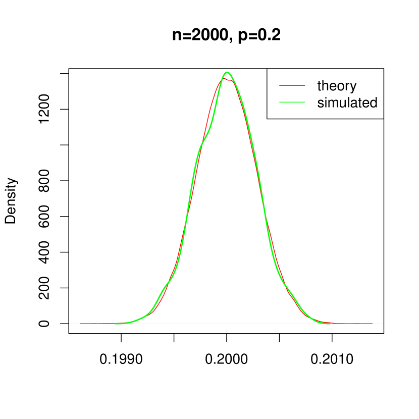
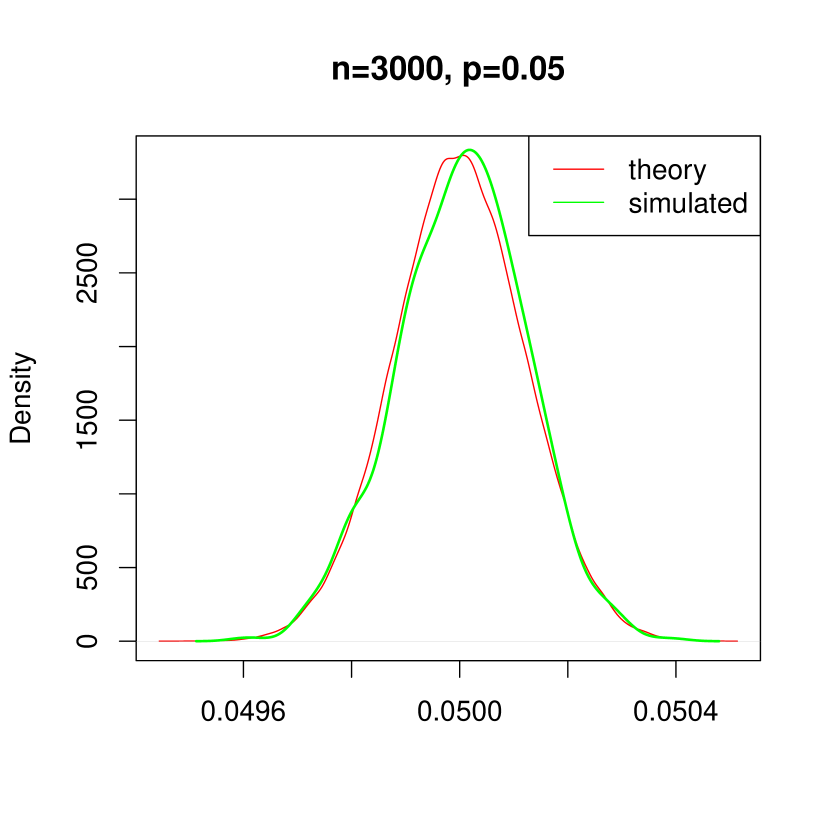
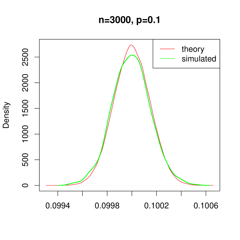
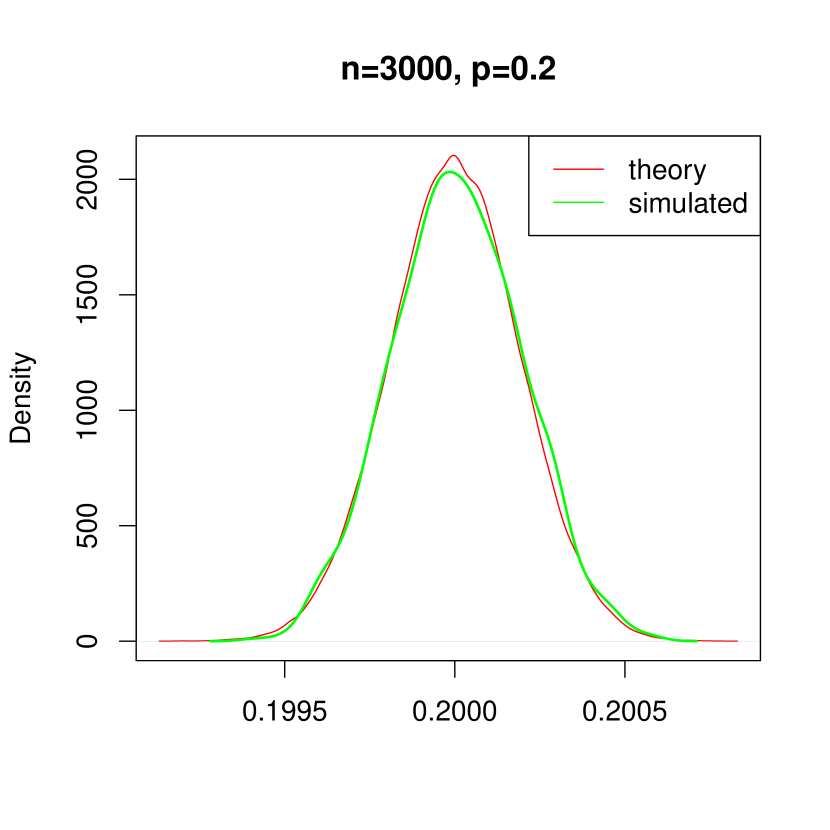
Figure 1: The derived asymptotic distribution of $C$ in ER graph compared with observed distribution of $C$ in 100000 simulations from the ER model.

Asymptotic test with ER null model

We also propose an asymptotic test with the test statistic in Equation 3.1 and ER as null model. We estimate the parameter $p=\frac{2\delta}{n-1}$ in the ER model with the observed network density, $\hat{p}=\frac{2\sum_{i<j}A_{ij}}{n(n-1)}$.

Define the matrix

$$\Sigma=3(n-2)\binom{n}{3}p(1-p)\begin{pmatrix}4p^{2}+\frac{p(1-p)}{n-2}&2p^{3}+\frac{p^{2}(1-p)}{n-2}\\ 2p^{3}+\frac{p^{2}(1-p)}{n-2}&p^{4}+\frac{p^{2}(1+p-2p^{2})}{3(n-2)}\end{pmatrix},$$

and let $\hat{\Sigma}$ be the plug-in estimator of $\Sigma$ obtained by replacing $p$ with $\hat{p}$ in the definition of $\Sigma$.

We propose to use the following rejection cutoffs for the test with level at most $\alpha$.

1. $K_{\alpha}$ is the $100*(1-\alpha)$th quantile of the distribution

   $$\text{LogNormal}\left(\log(\hat{p}),\frac{1}{\binom{n}{3}^{2}}\left(\frac{\hat{\Sigma}_{22}}{\hat{p}^{6}}+\frac{\hat{\Sigma}_{11}}{9\hat{p}^{4}}-2\frac{\hat{\Sigma}_{12}}{3\hat{p}^{5}}\right)\right)$$ (3.2)

2. $K_{2}$ is $\frac{(2+\epsilon)\log(n)}{\log(n\hat{p})}$ for any $\epsilon>0$. We use $\epsilon=0.0001$ in our experiments.

First we have the following result characterizing the asymptotic null distribution of $C$ under the ER null model. We derive this result using the multivariate delta technique based on well-known multivariate central limit theorem results on subgraph counts of random graphs Gao and Lafferty, (2017); Nowicki and Wierman, (1988); Janson and Nowicki, (1991); Reinert and Röllin, (2010).

Theorem 1.

Assume $p$ is fixed and does not vary with $n$. Under the null hypothesis we have the following asymptotic distribution for $C$,

$$C\to\text{LogNormal}\left(\log(p),\frac{1}{\binom{n}{3}^{2}}\left(\frac{\Sigma_{22}}{p^{6}}+\frac{\Sigma_{11}}{9p^{4}}-2\frac{\Sigma_{12}}{3p^{5}}\right)\right)$$

The next two results characterize the asymptotic level and power of the test on $C$ and $L$ whose proves are based on concentration inequalities.

Theorem 2.

Let $K_{\alpha}$ be the cutoff as defined in 3.2. Then

1. $P(C>K_{\alpha})\to\alpha,\text{ when }A\sim ER(n,p)$

2. $P(C>K_{\alpha})\rightarrow 1,\text{ when }A\sim NW(n,p,\beta)$

as $n\rightarrow\infty.$

Theorem 3.

Suppose $\frac{np}{\log(n)}\rightarrow\infty$ as $n\rightarrow\infty$, and $p<1/4.$ Then, in this range of $p$, using $K_{2}=\frac{(2+\epsilon)\log(n)}{\log(n\hat{p})}$, we have

1. $P[L>K_{2}]\rightarrow 0$ when $\beta=0$, i.e., $A\sim ER(n,p)$,

2. $P[L>K_{2}]\rightarrow 0$ when $A\sim NW(n,p,\beta)$ for some $0<\beta<1$,

3. $P[L>K_{2}]\rightarrow 1$ when $\beta=1$, i.e., $A$ is a ring lattice.

The proofs of these three theorems can be found in the supplementary materials.

Weak small world property

Our simulation results show that the empirical values of average path lengths is highly concentrated around their mean for all the null models. Therefore, many networks end up being not small world in our bootstrap test because the observed average path length is higher than even very high percentiles of what the null models predict. On the other hand we note that in the asymptotic test with ER null model, the cut off $K_{2}$ is roughly twice the average path length of an ER random graph. Motivated by these observations we define another concept of weak small world property that might be of descriptive aid. The weak small property has the value of $K_{1}$ (namely 95th quantile of the null model distribution of $C$), but the value of $K_{2}$ is twice the average path length observed in simulated networks. While our small-world property test provides an overall p-value for the test, the weak small world property has an associated p-value only for the first part of the test involving $C$ and only a decision associated with the second part of the test involving $L$. The asymptotic test defined in the last section detects the weak small world property with ER null models. This is the first procedure to detect a small-world property that does not require sampling new networks and therefore is easily scalable to large networks.

4 Simulation

4.1 Asymptotic distribution of $C$ in Theorem 1

To verify the asymptotic distribution of $C$ under the ER model derived in Theorem 1, we generate 100000 random graphs each from the 12 ER models varying $n=(500,1000,2000,3000)$ and $p=(0.05,0.1,0.2)$ and compute the clustering coefficient ($C$) in each case. Then we compare the observed distribution of the values of $C$ in the simulated graphs with our asymptotic distribution in Figure 1. The theoretical asymptotic distribution matches the simulated one closely for all values of $n$ and $p$ indicating that the derived distribution is a good fit.

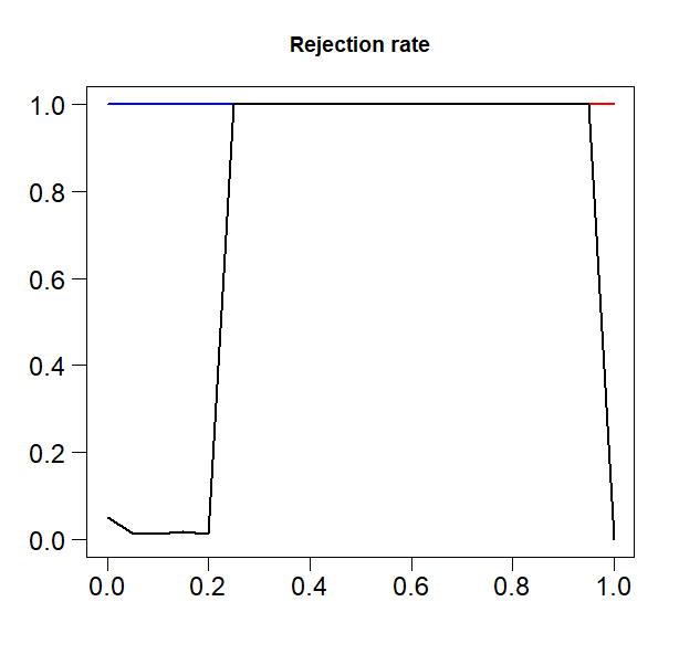
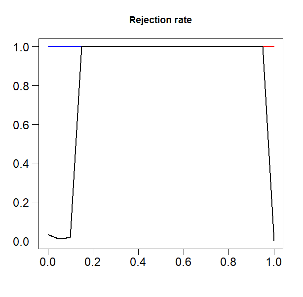
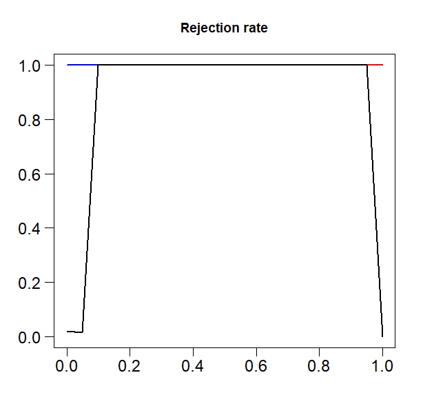
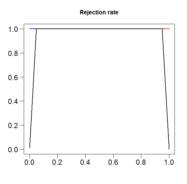
Figure 2: Power curves for the asymptotic test with $n$ fixed at 1000, and average degree being $10,20,40,50$ from left to right. The X-axis represents values of $\beta$. The red curve represents the observed rate of the clustering rule, i.e., $P[C>K_{1}]$, the blue curve represents the observed rate of the APL rule, i.e., $P[L<K_{2}]$, while the black curve represents the rejection rate of the intersection test, i.e., $P[C>K_{1},L<K_{2}]$.

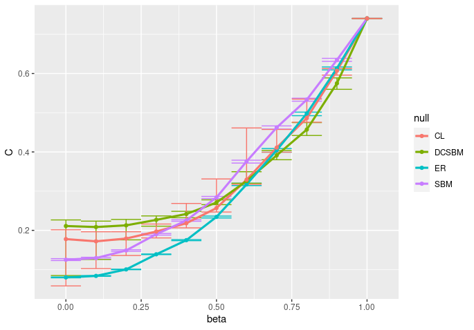
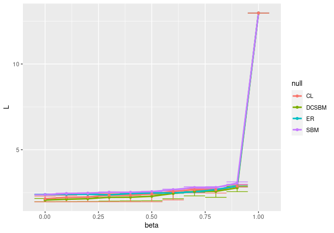
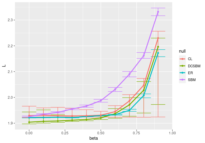
Figure 3: Median along with 1% and 99% quantiles for observed distribution of $C$ and $L$ with increasing $\beta$ for ER, CL, SBM, and DCSBM.

4.2 Power of the asymptotic test

Next we verify the power of the asymptotic test described through Theorems 2 and 3. We fix $n=1000$ and vary the average degree (which is $2\delta$) as $10,20,30,40,50$. The power curves against changing $\beta$ using the asymptotic test are shown in Figure 2. From the figure we note that both at $\beta=0$ and $\beta=1$, the rejection rate of the test is close to 0. The rejection rate curve (power curve) sharply increases to 1 after sufficiently large $\beta$ and stays close to 1 until $\beta=1$. As the average degree increases, the sharp increase in the power curve starts for $\beta$ closer to 0, and at $2\delta=50$, the power curve is close to 0 for almost all value of $\beta$ in between 0 and 1.

4.3 Distribution of $C$ and $L$ for different null model

Next we design a simulation to understand how the distribution of $C$ and $L$ changes with increasing $\beta$ for more general null models. To do so we generate data from the superimposed Newman Watts models with ER, CL, SBM and DCSBM null models by varying $\beta$. We keep $n=1000$ and $2\delta=80$ and generate 250 networks for each $\beta$ value. Figure 3(a) and (b) presents the median along with 1% and 99% quantiles of the observed values of $C$ and $L$ over these 250 networks respectively. Figure 3(c) is the same figure as Figure 3(b), but without $\beta=1$ to better observe the differences for smaller $\beta$ values. We make a number of observations from these figures. First, as $\beta$ increases both the 1% and 99% quantiles of $C$ values steadily increases for all null models and the 1% quantiles quickly becomes larger than the 99% quantiles of $\beta=0$. On the other hand for $L$ the increase in the 1% and 99% quantiles is slower with increasing $\beta$, and in fact the 1% quantiles remain smaller than the 99% quantiles of $\beta=0$ for many values of $\beta$ until eventually at $\beta=1$, the values increase rapidly. This gives credence to the fact that there is a range of $\beta$ values $C$ is large compared to $\beta=0$ while $L$ is comparable to $\beta=0$. Second, we find differences in behavior of the different null models. Both $C$ and $L$ are highly concentrated around their median for the Newman Watts model with ER null model for all values of $\beta$. However for null models which account for degree heterogeneity, i.e., CL and DCSBM, the intervals between 1% and 99% quantiles are quite large. This is especially the case for $L$. Therefore for CL null model we note that there is a large range of $\beta$ values for which 1% quantile of $C$ is larger than 99% quantile of $\beta=0$, while the 1% quantile of $L$ is smaller than the 99% quantile of $\beta=0$.

5 Results on real networks

Null	C	L	Decision
ER	0	0.99	Reject
SBM	0	0.016	Reject
DCSBM	0	0	Reject
CL	0	0.06	Reject

(a) C Elegans

Null	C	L	Decision
ER	0	1	Fail to reject
SBM	0	0.932	Reject
DCSBM	0	0.854	Reject
CL	0	0.968	Reject

(b) Dolphins

Null	C	L	Decision
ER	0	1	Fail to reject
SBM	0.002	0.668	Reject
DCSBM	0	0	Reject
CL	0	1	Fail to reject

(c) Football

Null	C	L	Decision
ER	0	0.536	Reject
SBM	0.376	0.058	Fail to reject
DCSBM	0.012	0.018	Reject
CL	0.652	0.164	Fail to reject

(d) Karate

Null	C	L	Decision
ER	0	0.982	Reject
SBM	0	0.006	Reject
DCSBM	0	0.006	Reject
CL	0	0.028	Reject

(e) Les Miserables

Null	C	L	Decision
ER	0	1	Fail to reject
SBM	0	1	Fail to reject
DCSBM	0	0.9	Reject
CL	0	1	Fail to reject

(f) Macaque Cortex

Null	C	L	Decision
ER	0	1	Fail to reject
SBM	0	0	Reject
DCSBM	0	0.036	Reject
CL	0	0	Reject

(g) Political Blogs

Null	C	L	Decision
ER	0	1	Fail to reject
SBM	0	1	Fail to reject
DCSBM	0	0.99	Reject
CL	0	1	Fail to reject

(h) Political Books

Null	C	L	Decision
ER	0	1	Fail to reject
SBM	0	0.672	Reject
DCSBM	0	0.986	Reject
CL	0	1	Fail to reject

(i) Power Grid

Null	C	L	Decision
ER	0	0.508	Reject
SBM	0	0.22	Reject
DCSBM	0	0.032	Reject
CL	0.972	0.012	Fail to reject

(j) Word Adjacencies

Table 2: Results of the bootstrap intersection test on real world networks.

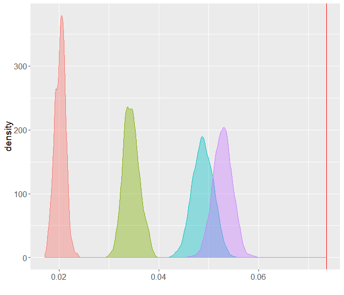
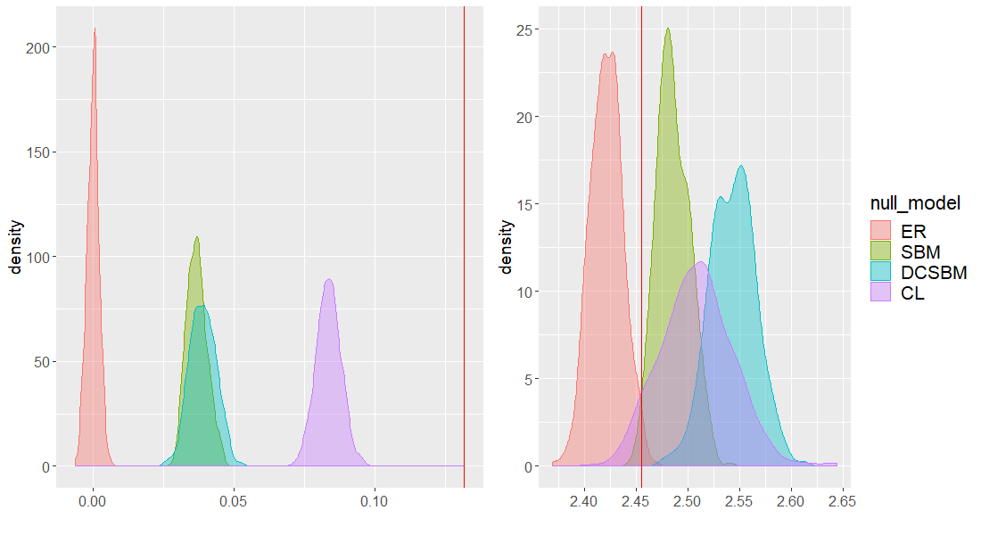
(a) C.Elegans White et al., (1986); Watts and Strogatz, (1998)

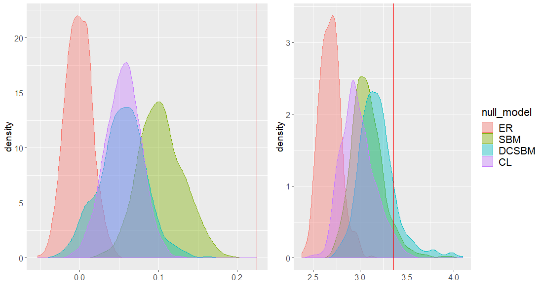
(b) Dolphins Lusseau et al., (2003)

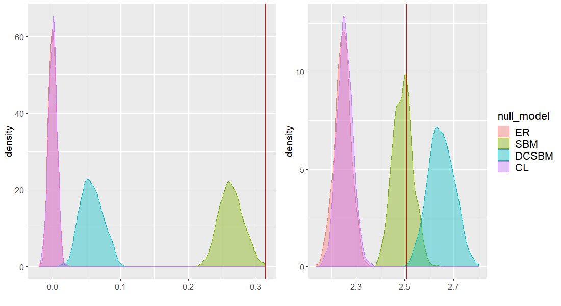
(c) Football Girvan and Newman, (2002)

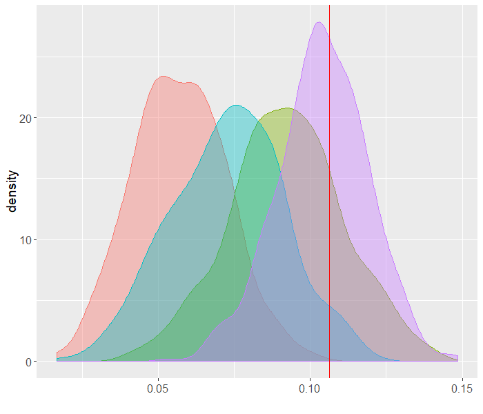
(d) Karate Club network Zachary, (1977)

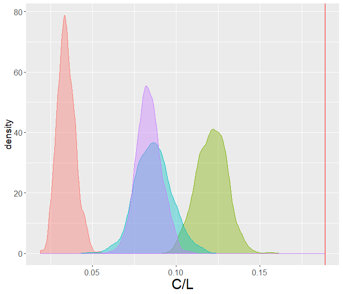
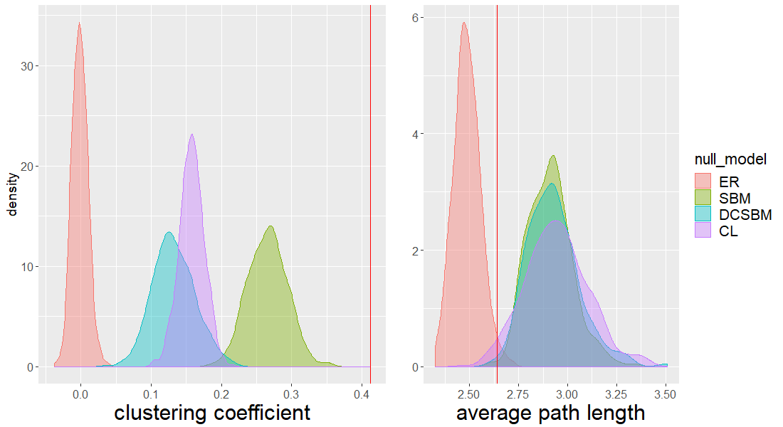
(e) Les Miserables Knuth, (1993)

Figure 4: Bootstrap tests on real-world networks. The first figure in each row is the empirical distributions of the small-world coefficient, second shows empirical distributions for the clustering coefficient and the average path length. 500 simulations were used to generate the distributions for ER, SBM, DCSBM and CL null models. The red line in both figures is the observed test-statistic.

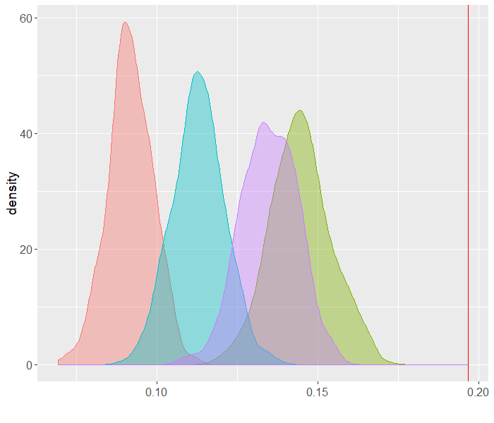
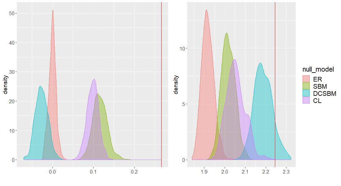
(a) Macaque Cortex Kaiser and Hilgetag, (2006)

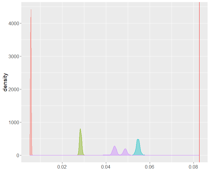
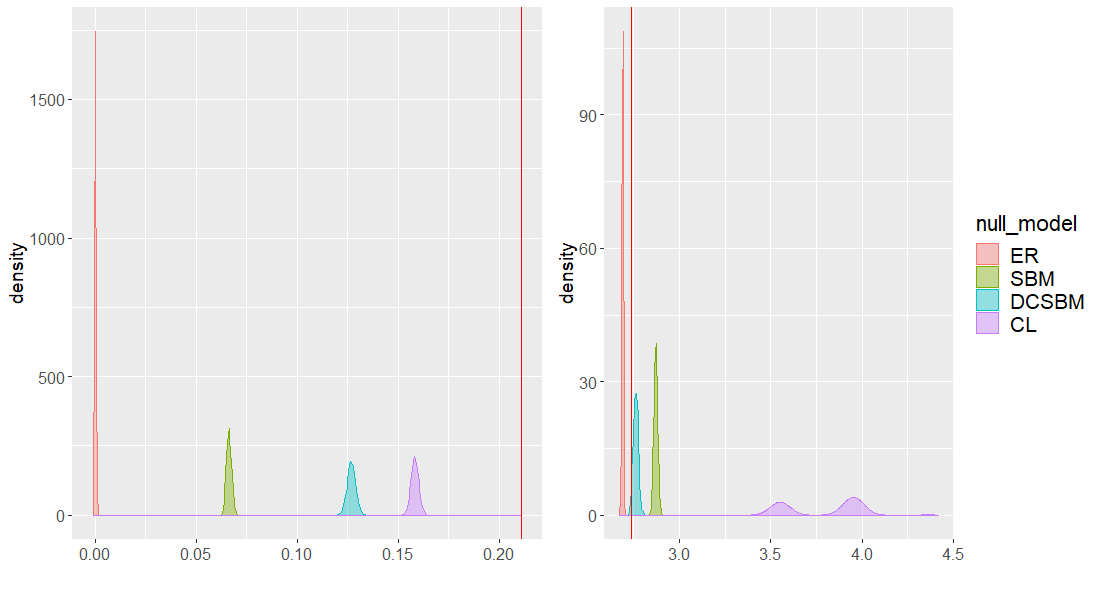
(b) Political Blogs Adamic and Glance, (2005)

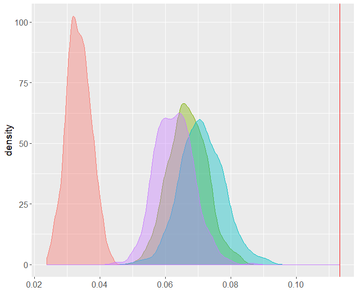
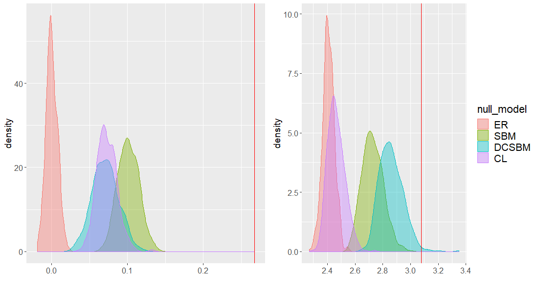
(c) Political Books (V.Kreb (www.orgnet.com))

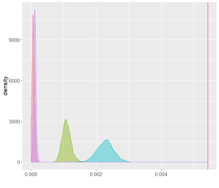
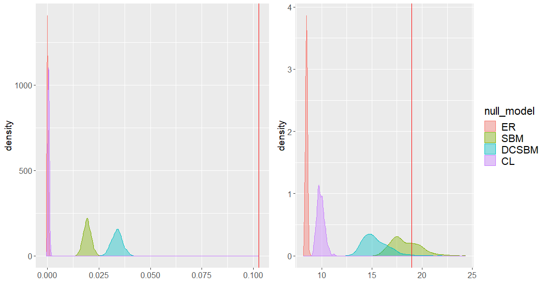
(d) Power Grid Watts and Strogatz, (1998)

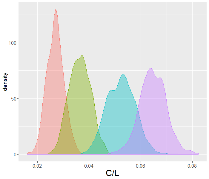
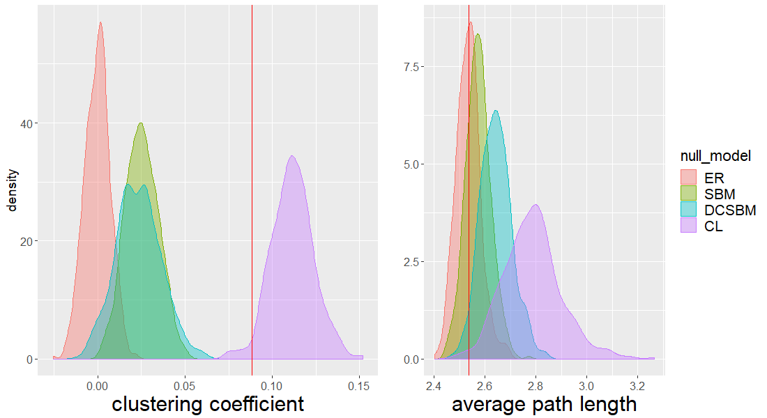
(e) Word Adjacency Newman, (2006)

Figure 5: Bootstrap tests on real-world networks continued.

Null	$K_{C}$	$K_{L}$	Decision
ER	0.039	4.255	Reject
SBM	0.043	4.971	Reject
DCSBM	0.047	5.087	Reject
CL	0.090	5.017	Reject

(a) C Elegans $\,C=0.132,\,L=2.455$

Null	$K_{C}$	$K_{L}$	Decision
ER	0.034	4.99	Reject
SBM	0.153	6.164	Reject
DCSBM	0.099	6.371	Reject
CL	0.091	5.958	Reject

(b) Dolphins $\,C=0.225,\,L=3.357$

Null	$K_{C}$	$K_{L}$	Decision
ER	0.012	3.995	Reject
SBM	0.293	4.983	Reject
DCSBM	0.086	5.298	Reject
CL	0.009	4.509	Reject

(c) Football $\,C=0.314,\,L=2.508$

Null	$K_{C}$	$K_{L}$	Decision
ER	0.068	4.541	Reject
SBM	0.179	5.303	Fail to reject
DCSBM	0.084	5.629	Reject
CL	0.197	5.289	Fail to reject

(d) Karate $\,C=0.117,\,L=2.408$

Null	$K_{C}$	$K_{L}$	Decision
ER	0.024	4.573	Reject
SBM	0.311	5.820	Reject
DCSBM	0.184	5.853	Reject
CL	0.187	5.889	Reject

(e) Les Miserables $\,C=0.414,\,L=2.641$

Null	$K_{C}$	$K_{L}$	Decision
ER	0.019	3.374	Reject
SBM	0.144	4.034	Reject
DCSBM	-0.003	4.376	Reject
CL	0.120	4.108	Reject

(f) Macaque Cortex $\,C=0.266,\,L=2.245$

Null	$K_{C}$	$K_{L}$	Decision
ER	0.0006	4.696	Reject
SBM	0.068	5.741	Reject
DCSBM	0.130	5.521	Reject
CL	0.1613	7.591	Reject

(g) Political Blogs $\,C=0.211,\,L=2.737$

Null	$K_{C}$	$K_{L}$	Decision
ER	0.015	4.354	Reject
SBM	0.124	5.455	Reject
DCSBM	0.099	5.722	Reject
CL	0.095	4.929	Reject

(h) Political Books $\,C=0.267,\,L=3.079$

Null	$K_{C}$	$K_{L}$	Decision
ER	0.0008	17.324	Fail to reject
SBM	0.026	36.747	Reject
DCSBM	0.038	30.763	Reject
CL	0.001	19.818	Reject

(i) Power Grid $\,C=0.103,\,L=18.989$

Null	$K_{C}$	$K_{L}$	Decision
ER	0.015	4.636	Reject
SBM	0.041	5.146	Reject
DCSBM	0.045	5.286	Reject
CL	0.132	5.571	Fail to reject

(j) Word Adjacency $\,C=0.089,\,L=2.536$

Table 3: Results from Weak Small-world test. For each network we present the cutoffs $K_{C}$ and $K_{L}$ for each null model. A network is weak small world under a specific null model if the observed $C$ is greater than $k_{C}$ and the observed $L$ is less than $K_{L}$.

We apply the bootstrap detection method for small world property to several real-world networks using the above-mentioned four null models, namely ER, SBM, DCSBM and CL. For each null model, we generate 500 networks to derive empirical distributions of $C$ and $L$ using parameters learned from a given real-world network. We present these empirical distributions for 10 real network datasets in the right columns of Figures  4 and  5. The observed values of $C$ and $L$ are indicated in the Figures with a red colored vertical line. In Table  2 we further present p-values associated with the two components of our intersection test statistic in Equation 3.1, as well as the overall decision from out test. In the table  2, the column for $C$ depicts $\mathbf{p_{C}}$, which is the proportion of simulated networks which have a higher clustering coefficient, and the column for $L$ depicts $\mathbf{p_{L}}$ , which is the proportion of simulated networks which have a lower average path length. The Decision column present the verdict from the the intersection test which rejects the null hypothesis to conclude that a given network is small-world, if the null hypothesis for both $C$ and $L$ are rejected. The test for $C$ rejects the null if $\mathbf{p_{C}}<0.05$, indicating that the given network has a significantly higher clustering coefficient compared to the null model. The test for $L$ rejects the null if $\mathbf{p_{L}}<0.99$, indicating the given network has a comparable path length to the null model. Finally, the left columns of Figure 4 and 5 further depicts the empirical distribution of the test statistic $\mathbf{C/L}$ along with its observed value.

Several interesting features emerge from our results. From Figure 4, the C-elegans and Les Miserables networks are small world under all four null models. The Karate club network is not small world under SBM and CL null models because the clustering coefficient $C$ is not significantly higher than what the two null models predict, despite $L$ being within the distribution of $L$ from all the null models. Therefore, the Karate club network’s high clustering coefficient can be well explained by either community structure or degree heterogeneity. On the other hand the Football network is not small world under ER and CL null models and the Dolphin network is not small world under the ER model, because the average path length $L$ is not within the distribution of $L$ from the null model. In both the networks, the clustering coefficient $C$ is higher than what any of the null models would predict. For both the networks the average path length is high enough that a ER random graph model cannot explain it. However, such an average path length can be well predicted by models that include community structure and/or degree heterogeneity.

In Figure 5, none of the 5 networks is small world under all four null models. The Macaque Cortex and Political books networks are small world only under DCSBM null model. For the other three null models, the distribution of $L$ values is completely in the left hand side of the observed $L$ value. The power grid, political blogs, and political books networks have very high observed values of $C$ which is higher than what any of the null models would predict. Therefore, in terms of clustering, the networks cannot be well approximated by any of the null models and require models with additional features. However, $L$ is comparable to only SBM and DCSBM null models for power grid network, SBM, DCSBM and CL null models for political blogs and DCSBM for political books networks. The word adjacencies network has a $C$ which is lower than the distribution of $C$ from the CL model and therefore it is not small world under the CL model. The network is small world under all other null models. Only the CL model can explain both the high clustering coefficient and the low average path length for this network.

Overall it appears that many networks are able to “pass” (i.e., reject) the clustering coefficient test for most of the null models, but “fail” (i.e., fail to reject) the average path length rest for some null models. Clearly the more complex null models, namely, CL and DCSBM consistently predicts higher average path length than the ER random graph model and are able to model the observed path lengths in many cases. Therefore many networks are small world only under those models and not under the SBM and ER models. This is an useful finding in terms of modeling choice for real-world network data.

Further, as the left columns of the Figures 4 and 5 show, the results with the traditional small world coefficient is identical to the result one would obtain from the clustering coefficient test alone. Consequently, using the traditional coefficient fails to take into account the average path length of the observed networks. This is contradictory to the philosophical spirit of the small world phenomenon - clustering structure despite small average path length. Consequently with ER null model the traditional small world coefficient declares all networks under test as small world. With SBM the metric only detects the Karate Club network as not being small world, with CL it detects Karate and word adjacencies as not small world, while with DCSBM it again detects all networks as small world. In comparison results with our proposed methodology brings out consequences of various modeling choices and help distinguish small-world property from community structure and degree heterogeneity.

Finally, we present the results from the “Weak small-world property” in Table 3. In each case we present the cutoff values for rejection for $K_{C}$ and $K_{L}$ under different null models. We will call a network small world if the observed value of $C$ is greater than the cutoff $K_{C}$ and the observed value of $L$ is less than the cutoff $K_{L}$. For the ER null model the cutoff $K_{C}$ is the theoretical $95th$ quantile of the asymptotic distribution of $C$ derived in 1, while the cutoff $K_{L}$ is the value $K_{2}$ defined in Theorem 3. For other null models we approximate these expected values with the 95th quantile of the bootstrap null distribution of $C$ and twice the average path length in the bootstrap null distribution of $L$ respectively. We note that for all real world networks and almost all null models, the observed value of $L$ is less than the small-world cutoff of twice the average expected path length (except for Power grid network with ER null model). The observed value of $C$ is also almost universally higher than the cutoff except for Karate Club network with SBM and CL null models and Word adjacency network with CL null model. In particular we note that while many networks are not deemed to be (strong) small-world in Table 2 because their observed average path lengths are higher than even the high quantiles of the distribution of average path length, they are deemed (weak) small-world because their observed path lengths are within twice the expected average path length. This observation is in-line with our observation in simulation (Figure 3 that the distribution of $L$ is highly concentrated around its mean.

6 Limitations and Conclusions

We have developed a hypothesis testing framework for detecting the small world property of network by defining suitable null and alternative family of models and hypotheses. The test is an intersection of two tests on average path length and clustering coefficient, which is rejected (network is designated small-world) if both the tests are rejected simultaneously. Our empirical results bring out interaction between average path length and clustering coefficient in real networks which places them closer to one of the different random graph null models we employ.

Acknowledgment

This work was supported in part by National Science Foundation grant DMS-1830547 and the NIH grant 7R01LM013309.

Appendix: Proofs

6.1 Proof of Theorem 1

We re-write the Proposition 2 of Reinert and Röllin, (2010) (also see Janson and Nowicki, (1991)) with a slight modification as

$$\sqrt{n}\begin{pmatrix}\frac{1}{\sqrt{n}n^{2}}(S-E[S])\\ \frac{1}{\sqrt{n}n^{2}}(T-E[T])\end{pmatrix}\,\overset{D}{\rightarrow}\,\mathcal{MVN}_{2}(0,\frac{1}{n^{4}}\Sigma),$$

where

$$\Sigma=3(n-2)\binom{n}{3}p(1-p)\begin{pmatrix}4p^{2}+\frac{p(1-p)}{n-2}&2p^{3}+\frac{p^{2}(1-p)}{n-2}\\ 2p^{3}+\frac{p^{2}(1-p)}{n-2}&p^{4}+\frac{p^{2}(1+p-2p^{2})}{3(n-2)}\end{pmatrix}$$

Clearly all elements of $\frac{1}{n^{4}}\Sigma$ are $O(p^{3})$ and therefore none of them diverges with increasing $n$. Consequently we have

$$\begin{pmatrix}\frac{1}{\sqrt{n}n^{2}}(S-E[S])\\ \frac{1}{\sqrt{n}n^{2}}(T-E[T])\end{pmatrix}\,=o(1)O_{p}(1)=o_{p}(1)$$

and then we can apply the multivariate delta method. We also note that the expectations are

$$E[T]=\binom{n}{3}p^{3},\quad\quad E[S]=3\binom{n}{3}p^{2}$$

Consider the function

$$g(X_{1},X_{2})=\log\left(\frac{3X_{2}}{X_{1}}\right)=\log(3X_{2})-\log(X_{1}).$$

Clearly this is a continuous function at $\mu=\frac{1}{\sqrt{n}n^{2}}[E[S],E[T]]$. Then from the intermediate value theorem we have

$$\sqrt{n}\left(g(\frac{1}{\sqrt{n}n^{2}}[S\quad T]^{T})-g(\frac{1}{\sqrt{n}n^{2}}[E[S]\quad E[T]]^{T})\right)$$

$$=\sqrt{n}[D(g(\mu))]\frac{1}{\sqrt{n}n^{2}}\left([S\quad T]^{T}-[E[S]\quad E[T]]^{T}\right)+o_{p}(1)$$

$$\to N_{2}\left(0,[D(g(\mu))]\frac{\Sigma}{n^{4}}[D(g(\mu))]^{T}\right),$$

where $D(g(\mu))$ is the matrix of first derivatives defined by

$$[D(g(\mu))]_{ij}=\frac{\partial g_{i}(\mu)}{\partial\mu_{j}}.$$

We note the function $g(\mu)$ is $\mathcal{R}^{2}\to\mathcal{R}$, and is given by

$$g(\mu)=\log(\frac{1}{\sqrt{n}n^{2}}3E[T])-\log(\frac{1}{\sqrt{n}n^{2}}E[S]).$$

Therefore,

$$[D(g(\mu))]=\left[-\frac{\sqrt{n}n^{2}}{E[S]}\quad\frac{3\sqrt{n}n^{2}}{3E[T]}\right].$$

and consequently,

$$[D(g(\mu))]\Sigma[D(g(\mu))]^{T}$$

$$=[-\frac{\sqrt{n}n^{2}}{E[S]}\quad\frac{\sqrt{n}n^{2}}{E[T]}]\begin{pmatrix}\Sigma_{11}&\Sigma_{12}\\ \Sigma_{12}&\Sigma_{22}\end{pmatrix}\begin{pmatrix}-\frac{\sqrt{n}n^{2}}{E[S]}\\ \frac{\sqrt{n}n^{2}}{E[T]}\end{pmatrix}$$

$$=n^{5}[\frac{\Sigma_{12}}{E[T]}-\frac{\Sigma_{11}}{E[S]},\,\frac{\Sigma_{22}}{E[T]}-\frac{\Sigma_{12}}{E[S]}]\begin{pmatrix}-\frac{1}{E[S]}\\ \frac{1}{E[T]}\end{pmatrix}$$

$$=n^{5}(-\frac{\Sigma_{12}}{(E[S])E[T]}+\frac{\Sigma_{11}}{(E[S])^{2}}+\frac{\Sigma_{22}}{E[T]^{2}}-\frac{\Sigma_{12}}{(E[S])E[T]})$$

$$=n^{5}(\frac{\Sigma_{11}}{(E[S])^{2}}+\frac{\Sigma_{22}}{E[T]^{2}}-2\frac{\Sigma_{12}}{(E[S])E[T]})$$

Therefore,

$$\sqrt{n}\left(\log C-\log(\frac{3E[T]}{E[S]})\right)$$

$$\to N\left(0,n(\frac{\Sigma_{22}}{E[T]^{2}}+\frac{\Sigma_{11}}{(E[S])^{2}}-\frac{2\Sigma_{12}}{E[S]E[T]})\right)$$

or equivalently,

$$\log C\to N(\log(\frac{3E[T]}{E[S]})),\frac{\Sigma_{22}}{E[T]^{2}}+\frac{\Sigma_{11}}{(E[S])^{2}}-\frac{2\Sigma_{12}}{E[S]E[T]})$$

and therefore $C$ converges to a log normal distribution.

6.2 Proof of Theorem 2:

Define $K^{\prime}_{\alpha}$ as the $100*(1-\alpha)$th upper quantile of the distribution of $C$ under the ER model with true value of $p$, i.e.,

$$K^{\prime}_{\alpha}=\exp\left(\log(p)+Z_{\alpha}\frac{1}{\binom{n}{3}^{2}}(\frac{\Sigma_{22}}{p^{6}}+\frac{\Sigma_{11}}{9p^{4}}-2\frac{\Sigma_{12}}{3p^{5}})\right),$$ (6.1)

where $Z_{\alpha}$ is the $100*(1-\alpha)$th upper quantile of the standard normal distribution. Let $K_{\alpha}$ be the corresponding $100*(1-\alpha)$th upper quantile that we calculate by replacing $p$ with the estimated value $\hat{p}$ in Equation 6.1. By weak law of large numbers

$$\hat{p}=\frac{2\sum_{i<j}A_{ij}}{n(n-1)}\quad\overset{p}{\to}\quad p,$$

and since $K_{\alpha}$ in Equation 6.1 is a continuous function of $p$, by the continuous mapping theorem,

$$K_{\alpha}\quad\overset{p}{\to}\quad K^{\prime}_{\alpha}\text{ as }n\to\infty.$$

Therefore,

$$P(C_{A}>K_{\alpha})\to\alpha,\text{ when }A\sim ER(n,\delta/(n-1)),$$

as $n\to\infty$.

Next we need to show that

$$P(C_{A}>K_{\alpha})\rightarrow 1,\text{ when }A\sim NW(n,p,\beta)\text{ and }n\rightarrow\infty.$$

We start proving this by defining the following three graphs:

• Let $A^{\prime}$ be an equivalent density ER graph, i.e., $A^{\prime}\sim ER(n,\delta/(n-1))$

• Let $A_{R}$ be the ring lattice component of the graph, i.e, obtained by removing the ER edges from the graph. In our notation, $A_{R}\sim RL(n,2\beta\delta)$ for some $0<\beta<1$, however this is a deterministic graph not a probabilistic one.

• Let $A_{E}$ be the Erdos Renyi component of the graph, i.e, obtained by removing the Ring lattice edges from the graph. In our notation, $A_{E}\sim ER(n,\frac{(1-\beta)d}{n-1})$ for some $0<\beta<1$.

Now since the number of triangles in $A$ must be higher than just the ring lattice portion of the graph $A_{R}$, we can say

$$C_{A}=\frac{T_{A}}{S_{A}}\geq\frac{T_{A_{R}}}{S_{A}}.$$

We use the Markov inequality on the non negative random variable $C_{A^{\prime}}$, which denotes the clustering coefficient of $A^{\prime}$, to state that, for any constant $c>0$ not dependent on $n$,

$$P\left(C_{A^{\prime}}\geq c\log n\frac{E[T_{A^{\prime}}]}{E[S_{A^{\prime}}]}\right)\leq\frac{1}{c^{\prime}\log n}\rightarrow 0,$$

as $n\rightarrow 0$, where $c^{\prime}$ is another constant not dependent on $n$. Therefore $K_{\alpha}$ above must satisfy

$$K_{\alpha}\leq c\log n\frac{E[T_{A^{\prime}}]}{E[S_{A^{\prime}}]}.$$

Therefore the desired result follows if we can prove that

$$P\left(T_{A_{R}}\geq cS_{A}\log n\frac{E[T_{A^{\prime}}]}{E[S_{A^{\prime}}]}\right)\rightarrow 1.$$ (6.2)

To show this we note that the quantities $T_{A_{R}},E[T_{A^{\prime}}],E[S_{A^{\prime}}]$ are all deterministic and calculate

$$T_{A_{R}}=n\dbinom{\delta\beta}{2}\asymp c_{2}n\delta^{2}\beta^{2},\quad\text{ and }\frac{E[T_{A^{\prime}}]}{E[S_{A^{\prime}}]}=c_{3}\frac{\delta}{n},$$

where $c_{2},c_{3}$ are constants independent of $n$. Therefore the result in Equation 6.2 is equivalent to

$$P\left(S_{A}\leq C_{2}\frac{n^{2}\delta\beta^{2}}{\log n}\right)\rightarrow 1.$$ (6.3)

We note $S_{A}$ consists of three parts:

$$S_{A}=\sum_{i,j,k}\{(S_{A_{E}})_{ijk}+(S_{A_{R}})_{ijk}+(E_{A_{E}})_{ij}(E_{A_{R}})_{jk}\}.$$

The middle term is a deterministic quantity and is upper bounded by

$$S_{A_{R}}=\frac{n.2\delta\beta(2\delta\beta-1)}{2}\leq c_{4}n\delta^{2}\beta^{2}.$$

By assumption of $\frac{\delta\log n}{n}\rightarrow 0$, (i.e., the graph is not too dense), we have

$$S_{A_{R}}<C_{2}\frac{n^{2}\delta\beta^{2}}{\log n}.$$

Next we derive an upper bound for the first term which holds with high probability. First note the expectation is,

$$E[S_{A_{E}}]=\frac{n(n-1)(n-2)}{2}\frac{4\delta^{2}(1-\beta)^{2}}{(n-1)^{2}}\asymp 2n\delta^{2}(1-\beta)^{2}$$

and

$$P(|S_{A_{E}}-E[S_{A_{E}}]|\geq\epsilon E[S_{A_{E}}])\leq\frac{c_{5}n\delta^{3}(1-\beta)^{3}}{n^{2}\delta^{4}(1-\beta)^{4}}=\frac{c_{5}}{n\delta(1-\beta)}.$$

Therefore,

$$P(S_{A_{E}}\leq c_{6}n\delta^{2}(1-\beta)^{2})\geq 1-\frac{c_{5}}{n\delta(1-\beta)},$$

where $c_{5},c_{6}$ are constants independent of $n$. By our assumption of $\frac{\delta\log n}{n}\rightarrow 0$,

$$c_{6}n\delta^{2}(1-\beta)^{2})<c_{7}\frac{n^{2}\delta\beta^{2}}{\log n}.$$

Finally, we tackle the third term. Note that the quantities $(E_{A_{R}})_{jk}$ are deterministic and we precisely know there are $n\delta\beta$ such edges. These incidental structures are formed if there is an ER edge in either end of the RL edge. Let $(d_{E})_{i}$ denote the degree of $i$th node in the graph $A_{E}$ and $d_{\max}=\max_{i}(d_{E})_{i}$ is the maximum degree of a node in $A_{E}$. Then from Bernstein inequality we get

$$P((d_{E})_{i} \geq(1+c_{8})\delta(1-\beta))$$

$$\leq\exp\left(-\frac{\frac{1}{2}c_{8}^{2}\delta^{2}(1-\beta)^{2}}{(n-2)\frac{\delta(1-\beta)}{n-1}(1-\frac{\delta(1-\beta)}{n-1})+\frac{1}{3}c_{8}\delta(1-\beta)}\right).$$

Taking an union bound over all $n$ vertices, we have

$$P(d_{\max}\geq(1+c_{8})\delta(1-\beta))\leq\exp(-c_{9}\log n).$$

Therefore we can bound the total number of incidental “V” shaped structures as

$$P\left(S_{A_{E}}\geq 2n\delta\beta(n-2)\frac{\delta(1-\beta)}{n-1}\right)\leq P\left(d_{\max}\geq(1+c_{8})\delta(1-\beta)\right)$$

and using the bound for the right hand side above we have

$$P\left(S_{A_{E}}\leq 2n\delta\beta(n-2)\frac{\delta(1-\beta)}{n-1}\right)\geq 1-\exp(-c_{9}\log n).$$

Next, combining the three results we have

$$P\left(S_{A}\leq C_{2}\frac{n^{2}\delta\beta^{2}}{\log n}\right)\geq 1-\frac{c_{1}0}{n\log n}-\exp(-c_{9}\log n)\rightarrow 1.$$ (6.4)

6.3 Proof of Theorem 3:

We start with some definitions. For any pair of nodes $(u,v)$, let $d(u,v)$ be the geodesic distance between $u$ and $v$. $\Gamma_{i}(v)$ is defined as the set of vertices at distance $i$ from vertex $v$, that is, $\Gamma_{i}(v)=\{u:d(u,v)=i\}$, and $|\Gamma_{i}(v)|$ is the number of vertices in the set $\Gamma_{i}(v)$.

Proof of Part 1: When $A\sim ER(n,p)$, our proof strategy is to collect the union of the events where $L>K_{2}$ can happen, and show that the sum of their probabilities go to zero. Define the following events:

1. The graph $G$ is not connected.

   It is well-known that $P[E1]\rightarrow 0$ when $\frac{np}{\log(n)}\rightarrow\infty$, which is our assumption. This result established by Erdös et al., (1959) is one of the most celebrated results in random graph theory. We skip the proof in the interest of space.

2. $\{\hat{p}>p(1+\frac{1}{\sqrt{n\log(n)}})\}$.

   We know that, for any $\epsilon\in(0,1)$, by Chernoff’s inequality,

   $$P[\hat{p}\geq(1+\epsilon)p]\leq\exp\left(-\frac{\epsilon^{2}{n\choose 2}p}{3}\right).$$

   Put $\epsilon=\frac{1}{\sqrt{n\log(n)}}$. Then, since ${\epsilon^{2}{n\choose 2}p}=\frac{(n-1)p}{2\log(n)}\rightarrow\infty$ by assumption, the probability on the right hand side goes to zero, which implies $P[E_{2}]\rightarrow 0$.

   (Note that we do not have to consider the case $\hat{p}<p$, since that makes $K_{2}$ larger than its population version, and therefore the right-tail probability is even lower.)

3. There is at least one vertex $v$ and some $i\in(1,\frac{2\log(n)}{3\log(np)})$ such that $|\Gamma_{i}(v)|\leq\frac{1}{2}(np)^{i}$.

   Here we apply Lemma 8 of Chung and Lu, (2001), which states that: when $p\geq\frac{c\log(n)}{n}$ for some $c>2$, then for any fixed vertex $v$, any fixed $i\in(1,\frac{2\log(n)}{3\log(np)})$, and any $\epsilon>0$,

   $$P[|\Gamma_{i}(v)|\leq(1-\sqrt{2/c}-\epsilon)(np)^{i}]=o\left(\frac{1}{n}\right).$$

   Fix any $\epsilon>0$. Since $\frac{np}{\log(n)}\rightarrow\infty$, we can use $c=\frac{2}{\epsilon^{2}}$, which implies that

   $$P[|\Gamma_{i}(v)|\leq(1-2\epsilon)(np)^{i}]=o\left(\frac{1}{n}\right).$$

   Taking union over $v$,

   $$P\left[\cup_{v\in(1,\ldots,n)}\left\{|\Gamma_{i}(v)|\leq\frac{1}{2}(np)^{i}\right\}\right]=o(1).$$

   Therefore, $P[E_{3}]\rightarrow 0$.

4. There exists a pair of vertices $(u,v)$, integers $k_{1},k_{2}$ such that

   $$|\Gamma_{k_{1}}(u)||\Gamma_{k_{1}}(v)|p>(2+\epsilon)\log(n)$$

   for some $\epsilon>0$, but $d(u,v)>k_{1}+k_{2}+1$.

   Suppose such a pair exists. There can be two cases.

   Case 1: $\Gamma_{k_{1}}(u)\cap\Gamma_{k_{2}}(v)$ is not null. Then, there is a path of length less than or equal to $k_{1}+k_{2}$ from $u$ to $v$, which means $d(u,v)\leq k_{1}+k_{2}$.

   Case 2: $\Gamma_{k_{1}}(u)\cap\Gamma_{k_{2}}(v)$ is null. Let’s compute the probability that there is no edge between $\Gamma_{k_{1}}(u)$ and $\Gamma_{k_{2}}(u)$. This probability is given by

   $$(1-p)^{|\Gamma_{k_{1}}(u)||\Gamma_{k_{1}}(v)|}.$$

   Note that $e^{-p}\geq(1-p)$. Therefore,

   $$(1-p)^{|\Gamma_{k_{1}}(u)||\Gamma_{k_{1}}(v)|} \leq\exp(-p|\Gamma_{k_{1}}(u)||\Gamma_{k_{1}}(v)|)$$

   $$\leq\exp(-(2+\epsilon)\log(n))=\frac{1}{n^{2+\epsilon}}.$$

   Therefore,

   $$P[\cup_{uv}\{\text{ No edge between }\Gamma_{k_{1}}(u)\text{ and }\Gamma_{k_{1}}(u)\}]\leq\frac{1}{n^{\epsilon}}\rightarrow 0.$$

   Therefore, $P[E_{4}]\leq\frac{1}{n^{\epsilon}}\rightarrow 0$.

Now, armed with the fact that $P[E1\cup E2\cup E3\cup E4]=0$, we proceed to complete the proof. Fix any $\epsilon>0$, and choose

$$k_{1}=\left\lceil\frac{\log(\sqrt{2(1+\epsilon)n\log(n)/(1-2\epsilon)})}{\log(np)}\right\rceil,$$

$$k_{2}=\left\lceil\frac{\log({2(1+\epsilon)n\log(n)/(1-2\epsilon)^{2}})}{\log(np)}-k_{1}-1\right\rceil.$$

Then $k_{1},k_{2}\in(1,\frac{2\log(n)}{3\log(np)})$, and therefore,

$$|\Gamma_{k_{1}}(u)||\Gamma_{k_{2}}(v)|\geq(1-2\epsilon)(np)^{k_{1}}\times(1-2\epsilon)(np)^{k_{2}}\geq 2(1+\epsilon)\log(n)$$

with probability greater than $1-P[E3]$. Therefore, from the result on E4, we can say that with probability $1-P[E3\cup E4]$, the path length between any two vertices is less than or equal to $k_{1}+k_{2}+1$. This implies that with probability $1-P[E3\cup E4]$, the average path length is less than or equal to $k_{1}+k_{2}+1$. Thus, we obtain

$$P\left[L\leq\left\lceil\frac{\log({2(1+\epsilon)n\log(n)/(1-2\epsilon)^{2}})}{\log(np)}\right\rceil\right]\rightarrow 1.$$

We can now conclude that, for any $\epsilon^{\prime}>0$,

$$P\left[L>\left\lceil\frac{\log({2(1+\epsilon^{\prime})n\log(n)})}{\log(np)}\right\rceil\right]\rightarrow 0.$$ (6.5)

However, $\lceil x\rceil$ could be anything from $x$ to $x+1$. Therefore, to be abundantly conservative, we use

$$\left\lceil\frac{\log({2(1+\epsilon^{\prime})n\log(n)})}{\log(np)}\right\rceil \leq\frac{\log({2(1+\epsilon^{\prime})n\log(n)})}{\log(np)}+1$$

$$=\frac{\log({2(1+\epsilon^{\prime})n^{2}p\log(n)})}{\log(np)}\leq\frac{(2+\delta)\log(n)}{\log(np)}$$

for any $\delta>0$. Finally, we have to adjust for the fact that $\hat{p}\leq p(1+\frac{1}{\sqrt{n\log(n)}})$, where we use the Taylor series approximation $\log(1+x)\approx x$ for the denominator. This gives us the final bound,

$$K_{2}=\frac{(2+\epsilon)\log(n)}{\log(n\hat{p})},$$

for any $\epsilon>0$.

Proof of Part 2:
When $A\sim NW(n,p,\beta)$, consider the network $A^{\prime}$ obtained by removing the ring lattice edges. Note that $A^{\prime}\sim ER(n,(1-\beta)p)$, so it follows from Equation (6.5) that

$$P\left[L(A^{\prime})>\frac{(2+\epsilon^{\prime})\log(n)}{\log((1-\beta)np)}\right]\rightarrow 0$$

for any $\epsilon^{\prime}>0$. Next, we prove that

$$P\left[K_{2}>\frac{(2+\epsilon^{\prime})\log(n)}{\log((1-\beta)np)}\right]\rightarrow 1$$

as $n\rightarrow\infty$. To see this, fix some $\epsilon\in(0,1)$, and let $K_{2}=\frac{(2+\epsilon)\log(n)}{\log(n\hat{p})}$. Let $\epsilon^{\prime}=\epsilon/2$, and let $K_{2}^{\prime}=\frac{(2+\epsilon^{\prime})\log(n)}{\log((1-\beta)np)}$. Then,

$$\frac{K_{2}}{K_{2}^{\prime}}=\frac{(2+\epsilon)\log((1-\beta)np}{(2+\epsilon/2)\log(n\hat{p})}=\frac{(2+\epsilon)}{(2+\epsilon/2)}\frac{\log(np)+\log(1-\beta)}{\log(np)+\log(\hat{p}/p)}.$$

Therefore, from the result on E2 from Part 1,

$$\frac{K_{2}}{K_{2}^{\prime}} =\frac{(2+\epsilon)}{(2+\epsilon/2)}\frac{\log(np)+\log(1-\beta)}{\log(np)+\log(1+\frac{1}{\sqrt{n\log(n)}})}$$

$$\geq \left(1+\frac{\epsilon}{6}\right)\frac{\log(np)+\log(1-\beta)}{\log(np)+\log(1+\frac{1}{\sqrt{n\log(n)}})}$$

with probability $1-P[E2]$. In the final expression, the first part is greater than 1, and the second part converges to 1 as $n\rightarrow\infty$, so we can choose $\epsilon$ to ensure that the product is greater than 1. Thus,

$$P\left[L(A^{\prime})>K_{2}\right]\leq P\left[L(A^{\prime})>K_{2}^{\prime}\right]+P[K_{2}<K_{2}^{\prime}]\rightarrow 0.$$

Clearly, $L(A)\leq L(A^{\prime})$, since $A$ has more edges than $A^{\prime}$, and every additional edge has a non-decreasing effect on the average path length. Therefore, we have proved part 2.

Proof of Part 3: For a ring lattice, we have

$$L\approx\frac{n}{2n\hat{p}}\approx\frac{1}{2{p}},\text{ and }K_{2}\approx\frac{(2+\epsilon)\log(n)}{\log(np)}$$

for large enough $n$ and small $\epsilon>0$. Therefore, it suffices to prove that for some $\epsilon>0$,

$$\frac{1}{2{p}}>\frac{(2+\epsilon)\log(n)}{\log(np)}$$

$$\Leftrightarrow\log(n)+\log(p)>2(2+\epsilon)p\log(n)$$

$$\Leftrightarrow\log(n)(1-2(2+\epsilon)p)+\log(p)>0,$$

which is true since $p<1/4$ and for large enough $n$.

References

- Adamic and Glance, (2005) Adamic, L. A. and Glance, N. (2005). The political blogosphere and the 2004 US election: divided they blog. In Proceedings of the 3rd International Workshop on Link Discovery, pages 36–43. ACM.
- Aiello et al., (2000) Aiello, W., Chung, F., and Lu, L. (2000). A random graph model for massive graphs. In Proceedings of the thirty-second annual ACM symposium on Theory of computing, pages 171–180.
- Albert and Barabási, (2002) Albert, R. and Barabási, A.-L. (2002). Statistical mechanics of complex networks. Reviews of modern physics, 74(1):47.
- Amaral et al., (2000) Amaral, L. A. N., Scala, A., Barthelemy, M., and Stanley, H. E. (2000). Classes of small-world networks. Proceedings of the national academy of sciences, 97(21):11149–11152.
- Ansmann and Lehnertz, (2011) Ansmann, G. and Lehnertz, K. (2011). Constrained randomization of weighted networks. Physical Review E, 84(2):026103.
- Bassett and Bullmore, (2006) Bassett, D. S. and Bullmore, E. (2006). Small-world brain networks. The neuroscientist, 12(6):512–523.
- Bassett et al., (2008) Bassett, D. S., Bullmore, E., Verchinski, B. A., Mattay, V. S., Weinberger, D. R., and Meyer-Lindenberg, A. (2008). Hierarchical organization of human cortical networks in health and schizophrenia. The Journal of Neuroscience, 28(37):9239–9248.
- Bassett and Bullmore, (2017) Bassett, D. S. and Bullmore, E. T. (2017). Small-world brain networks revisited. The Neuroscientist, 23(5):499–516.
- Bialonski et al., (2010) Bialonski, S., Horstmann, M.-T., and Lehnertz, K. (2010). From brain to earth and climate systems: Small-world interaction networks or not? Chaos: An Interdisciplinary Journal of Nonlinear Science, 20(1):013134.
- Bickel and Chen, (2009) Bickel, P. J. and Chen, A. (2009). A nonparametric view of network models and newman–girvan and other modularities. Proceedings of the National Academy of Sciences, 106(50):21068–21073.
- Blondel et al., (2008) Blondel, V. D., Guillaume, J.-L., Lambiotte, R., and Lefebvre, E. (2008). Fast unfolding of communities in large networks. Journal of Statistical Mechanics: Theory and Experiment, 2008(10):P10008.
- Bullmore and Sporns, (2009) Bullmore, E. and Sporns, O. (2009). Complex brain networks: graph theoretical analysis of structural and functional systems. Nature Reviews Neuroscience, 10(3):186–198.
- Chandrasekhar and Jackson, (2016) Chandrasekhar, A. and Jackson, M. O. (2016). A network formation model based on subgraphs. arXiv preprint arXiv:1611.07658.
- Chin et al., (2015) Chin, P., Rao, A., and Vu, V. (2015). Stochastic block model and community detection in sparse graphs: A spectral algorithm with optimal rate of recovery. In COLT, pages 391–423.
- Chung and Lu, (2001) Chung, F. and Lu, L. (2001). The diameter of sparse random graphs. Advances in Applied Mathematics, 26(4):257–279.
- Erdös et al., (1959) Erdös, P., Rényi, A., et al. (1959). On random graphs. Publicationes mathematicae, 6(26):290–297.
- Fortunato, (2010) Fortunato, S. (2010). Community detection in graphs. Physics reports, 486(3-5):75–174.
- Gallos et al., (2012) Gallos, L. K., Makse, H. A., and Sigman, M. (2012). A small world of weak ties provides optimal global integration of self-similar modules in functional brain networks. Proceedings of the National Academy of Sciences, 109(8):2825–2830.
- Gao and Lafferty, (2017) Gao, C. and Lafferty, J. (2017). Testing network structure using relations between small subgraph probabilities. arXiv preprint arXiv:1704.06742.
- Gao et al., (2017) Gao, C., Ma, Z., Zhang, A. Y., and Zhou, H. H. (2017). Achieving optimal misclassification proportion in stochastic block models. The Journal of Machine Learning Research, 18(1):1980–2024.
- Girvan and Newman, (2002) Girvan, M. and Newman, M. E. (2002). Community structure in social and biological networks. Proceedings of the National Academy of Sciences, 99(12):7821–7826.
- Guimera et al., (2005) Guimera, R., Mossa, S., Turtschi, A., and Amaral, L. N. (2005). The worldwide air transportation network: Anomalous centrality, community structure, and cities’ global roles. Proceedings of the National Academy of Sciences, 102(22):7794–7799.
- Guye et al., (2010) Guye, M., Bettus, G., Bartolomei, F., and Cozzone, P. J. (2010). Graph theoretical analysis of structural and functional connectivity mri in normal and pathological brain networks. Magnetic Resonance Materials in Physics, Biology and Medicine, 23(5-6):409–421.
- He et al., (2007) He, Y., Chen, Z. J., and Evans, A. C. (2007). Small-world anatomical networks in the human brain revealed by cortical thickness from mri. Cerebral cortex, 17(10):2407–2419.
- Hilgetag and Goulas, (2016) Hilgetag, C. C. and Goulas, A. (2016). Is the brain really a small-world network? Brain Structure and Function, 221(4):2361–2366.
- Hlinka et al., (2017) Hlinka, J., Hartman, D., Jajcay, N., Tomeček, D., Tintěra, J., and Paluš, M. (2017). Small-world bias of correlation networks: From brain to climate. Chaos: An Interdisciplinary Journal of Nonlinear Science, 27(3):035812.
- Hoff et al., (2002) Hoff, P. D., Raftery, A. E., and Handcock, M. S. (2002). Latent space approaches to social network analysis. Journal of the american Statistical association, 97(460):1090–1098.
- Humphries and Gurney, (2008) Humphries, M. D. and Gurney, K. (2008). Network ‘small-world-ness’: a quantitative method for determining canonical network equivalence. PloS one, 3(4):e0002051.
- Humphries et al., (2005) Humphries, M. D., Gurney, K., and Prescott, T. J. (2005). The brainstem reticular formation is a small-world, not scale-free, network. Proceedings of the Royal Society B: Biological Sciences, 273(1585):503–511.
- Janson and Nowicki, (1991) Janson, S. and Nowicki, K. (1991). The asymptotic distributions of generalized u-statistics with applications to random graphs. Probability theory and related fields, 90(3):341–375.
- Jeong et al., (2001) Jeong, H., Mason, S. P., Barabási, A.-L., and Oltvai, Z. N. (2001). Lethality and centrality in protein networks. Nature, 411(6833):41.
- Jeong et al., (2000) Jeong, H., Tombor, B., Albert, R., Oltvai, Z. N., and Barabási, A.-L. (2000). The large-scale organization of metabolic networks. Nature, 407(6804):651–654.
- Kaiser and Hilgetag, (2006) Kaiser, M. and Hilgetag, C. C. (2006). Nonoptimal component placement, but short processing paths, due to long-distance projections in neural systems. PLoS Comput Biol, 2(7):e95.
- Knuth, (1993) Knuth, D. E. (1993). The Stanford GraphBase: a platform for combinatorial computing, volume 1. AcM Press New York.
- Lei and Rinaldo, (2015) Lei, J. and Rinaldo, A. (2015). Consistency of spectral clustering in stochastic block models. The Annals of Statistics, 43(1):215–237.
- Liu et al., (2008) Liu, Y., Liang, M., Zhou, Y., He, Y., Hao, Y., Song, M., Yu, C., Liu, H., Liu, Z., and Jiang, T. (2008). Disrupted small-world networks in schizophrenia. Brain, 131(4):945–961.
- Lusseau et al., (2003) Lusseau, D., Schneider, K., Boisseau, O. J., Haase, P., Slooten, E., and Dawson, S. M. (2003). The bottlenose dolphin community of doubtful sound features a large proportion of long-lasting associations. Behavioral Ecology and Sociobiology, 54(4):396–405.
- Lynall et al., (2010) Lynall, M.-E., Bassett, D. S., Kerwin, R., McKenna, P. J., Kitzbichler, M., Muller, U., and Bullmore, E. (2010). Functional connectivity and brain networks in schizophrenia. The Journal of Neuroscience, 30(28):9477–9487.
- Meunier et al., (2010) Meunier, D., Lambiotte, R., and Bullmore, E. T. (2010). Modular and hierarchically modular organization of brain networks. Frontiers in neuroscience, 4:200.
- Milgram, (1967) Milgram, S. (1967). The small world problem. Psychology today, 2(1):60–67.
- Montoya and Solé, (2002) Montoya, J. M. and Solé, R. V. (2002). Small world patterns in food webs. Journal of theoretical biology, 214(3):405–412.
- Muldoon et al., (2016) Muldoon, S. F., Bridgeford, E. W., and Bassett, D. S. (2016). Small-world propensity and weighted brain networks. Scientific reports, 6:22057.
- Newman, (2001) Newman, M. E. (2001). The structure of scientific collaboration networks. Proceedings of the national academy of sciences, 98(2):404–409.
- Newman, (2006) Newman, M. E. (2006). Finding community structure in networks using the eigenvectors of matrices. Physical review E, 74(3):036104.
- Newman and Watts, (1999) Newman, M. E. and Watts, D. J. (1999). Scaling and percolation in the small-world network model. Physical Review E, 60(6):7332.
- Nowicki and Wierman, (1988) Nowicki, K. and Wierman, J. C. (1988). Subgraph counts in random graphs using incomplete u-statistics methods. Discrete Mathematics, 72(1-3):299–310.
- Pan and Sinha, (2009) Pan, R. K. and Sinha, S. (2009). Modularity produces small-world networks with dynamical time-scale separation. EPL (Europhysics Letters), 85(6):68006.
- Papo et al., (2016) Papo, D., Zanin, M., Martínez, J. H., and Buldú, J. M. (2016). Beware of the small-world neuroscientist! Frontiers in human neuroscience, 10:96.
- Paul et al., (2018) Paul, S., Milenkovic, O., and Chen, Y. (2018). Higher-order spectral clustering under superimposed stochastic block model. arXiv preprint arXiv:1812.06515.
- Reinert and Röllin, (2010) Reinert, G. and Röllin, A. (2010). Random subgraph counts and u-statistics: multivariate normal approximation via exchangeable pairs and embedding. Journal of Applied Probability, 47(2):378–393.
- Rohe et al., (2011) Rohe, K., Chatterjee, S., and Yu, B. (2011). Spectral clustering and the high-dimensional stochastic blockmodel. Ann. Statist, 39(4):1878–1915.
- Rubinov and Sporns, (2010) Rubinov, M. and Sporns, O. (2010). Complex network measures of brain connectivity: uses and interpretations. Neuroimage, 52(3):1059–1069.
- Sengupta and Chen, (2015) Sengupta, S. and Chen, Y. (2015). Spectral clustering in heterogeneous networks. Statistica Sinica, pages 1081–1106.
- Sengupta and Chen, (2018) Sengupta, S. and Chen, Y. (2018). A block model for node popularity in networks with community structure. Journal of the Royal Statistical Society: Series B (Statistical Methodology), 80(2):365–386.
- Sole and Montoya, (2001) Sole, R. V. and Montoya, M. (2001). Complexity and fragility in ecological networks. Proceedings of the Royal Society of London. Series B: Biological Sciences, 268(1480):2039–2045.
- Sporns, (2014) Sporns, O. (2014). Contributions and challenges for network models in cognitive neuroscience. Nature Neuroscience, 17(5):652–660.
- Telesford et al., (2011) Telesford, Q. K., Joyce, K. E., Hayasaka, S., Burdette, J. H., and Laurienti, P. J. (2011). The ubiquity of small-world networks. Brain connectivity, 1(5):367–375.
- Van Noort et al., (2004) Van Noort, V., Snel, B., and Huynen, M. A. (2004). The yeast coexpression network has a small-world, scale-free architecture and can be explained by a simple model. EMBO reports, 5(3):280–284.
- Vázquez, (2003) Vázquez, A. (2003). Growing network with local rules: Preferential attachment, clustering hierarchy, and degree correlations. Physical Review E, 67(5):056104.
- Wagner, (2001) Wagner, A. (2001). The yeast protein interaction network evolves rapidly and contains few redundant duplicate genes. Molecular biology and evolution, 18(7):1283–1292.
- Wagner and Fell, (2001) Wagner, A. and Fell, D. A. (2001). The small world inside large metabolic networks. Proceedings of the Royal Society of London. Series B: Biological Sciences, 268(1478):1803–1810.
- Watts and Strogatz, (1998) Watts, D. J. and Strogatz, S. H. (1998). Collective dynamics of small-world networks. Nature, 393(6684):440–442.
- White et al., (1986) White, J., Southgate, E., Thomson, J., and Brenner, S. (1986). The structure of the nervous system of the nematode caenorhabditis elegans: the mind of a worm. Phil. Trans. R. Soc. Lond, 314:1–340.
- Williams et al., (2002) Williams, R. J., Berlow, E. L., Dunne, J. A., Barabási, A.-L., and Martinez, N. D. (2002). Two degrees of separation in complex food webs. Proceedings of the National Academy of Sciences, 99(20):12913–12916.
- Zachary, (1977) Zachary, W. W. (1977). An information flow model for conflict and fission in small groups. Journal of anthropological research, 33(4):452–473.