BreakingBED - Breaking Binary and Efficient Deep Neural Networks by Adversarial Attacks

Abstract

Deploying convolutional neural networks (CNNs) for embedded applications presents many challenges in balancing resource-efficiency and task-related accuracy. These two aspects have been well-researched in the field of CNN compression. In real-world applications, a third important aspect comes into play, namely the robustness of the CNN. In this paper, we thoroughly study the robustness of uncompressed, distilled, pruned and binarized neural networks against white-box and black-box adversarial attacks (FGSM, PGD, C&W, DeepFool, LocalSearch and GenAttack). These new insights facilitate defensive training schemes or reactive filtering methods, where the attack is detected and the input is discarded and/or cleaned. Experimental results are shown for distilled CNNs, agent-based state-of-the-art pruned models, and binarized neural networks (BNNs) such as XNOR-Net and ABC-Net, trained on CIFAR-10 and ImageNet datasets. We present evaluation methods to simplify the comparison between CNNs under different attack schemes using loss/accuracy levels, stress-strain graphs, box-plots and class activation mapping (CAM). Our analysis reveals susceptible behavior of uncompressed and pruned CNNs against all kinds of attacks. The distilled models exhibit their strength against all white box attacks with an exception of C&W. Furthermore, binary neural networks exhibit resilient behavior compared to their baselines and other compressed variants.

1 Introduction

Neural network compression is an extensively studied topic for reducing the computational complexity [36, 27, 22], the memory demand [25, 20, 16] and/or the energy consumption [42] of deep neural networks (DNN) deployed on embedded systems. These aspects widen the potential for DNN applications in real-world scenarios. Particularly in the field of robotics and autonomous driving, increasingly deeper and larger convolutional neural networks (CNNs) are deployed on resource-constrained hardware platforms, enabling computer vision-based applications, such as pedestrian detection or free-space detection. Systems in autonomous vehicles are safety critical, maintaining zero-tolerance for potential threats to functional safety. Attacking (breaking) neural networks can be done by injecting small perturbations to their inputs, referred to as adversarial attacks [39]. Under the assumption of varying degrees of information on the CNN and the accessibility of its internal parameters, several black-box (GenAttack [2], LocalSearch [31]) and white-box (FGSM [12], DeepFool [30] and Carlini & Wagner [4]) attacks are potential threats. Understanding these threats helps to develop pro-active [11] and re-active [33] methods to defend against adversarial examples and thereby improve CNN robustness.

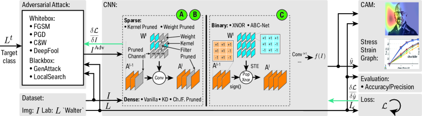
Figure 1: Experimental setup of BreakingBED for breaking binary (C) and efficient (A) and (B) DNNs attacked with white-box (FGSM, PGD and C&W) and black-box (LocalSearch and GenAttack) adversarial attacks. Evaluated by using loss/accuracy levels, stress-strain graphs, box-plots and class activation mapping (CAM).

Recent works investigated the mitigation of such threats through robust training of neural networks [15] and robust neural architecture search (NAS) techniques [13]. In [26], the authors compress neural networks through robust quantization, lowering the computational complexity while maintaining good performance against potential attacks. Further investigations on the robustness of binary neural networks (BNNs) were carried out in [10], where BNNs were attacked with white-box (FGSM [12] and C&W [4]) and black-box [34] techniques. The robustness of BNNs was concluded, albeit on basic adverserially trained networks from [34] and a small set of attacks.

In order to get a deeper understanding of the effectiveness of adversarial attacks (Sec. 3), applied to binary and efficient DNNs (Sec. 2), we perform an extensive set of robustness evaluation experiments. In detail, we expose vanilla full-precision, distilled, pruned and binary DNNs to a variety of adversarial attacks in Sec. 4.

2 Compression of Deep Neural Networks

Many works in literature have focused on reducing the redundancy emerging from training deeper and wider neural networks, aiming to mitigate the challenges of their deployment on edge devices. Compression techniques such as knowledge distillation, pruning, and binarization can potentially make CNNs more efficient in embedded settings.

2.1 Knowledge Distillation

Knowledge distillation (KD) is the transfer of knowledge from a teacher to a student network [40, 21]. The student can be a smaller DNN, which is trained on the soft labels of the larger teacher network, achieving an improvement in an accuracy-efficiency trade-off. The student represents a compressed version of the teacher, condensing its knowledge. This paper focuses on KD training, using Kullback-Leibler (KL) divergence between the teacher and the student output distribution formulated as the loss function in Eq. (1). Here, $\sigma(f_{t}(I))$ and $\sigma(f_{s}(I))$ represent the softmax output logits of the teacher and student network respectively, computed for a sample image $I$ in a mini batch of $N$ samples.

$$\small\hskip 14.22636pt\mathcal{L}^{KL}_{\text{KD}}(f_{t},f_{s},T)=\sum_{n=1}^{N}\sigma(f_{t}(I_{n})/T)\log\bigg{(}\frac{\sigma(f_{t}(I_{n})/T)}{\sigma(f_{s}(I_{n})/T)}\bigg{)}$$ (1)

During the knowledge transfer using the teacher’s logits, a softmax temperature $T\gg 1$ is used. During the evaluation, we use $T=1$ to obtain softmax-cross entropy loss.

2.2 Pruning

Pruning aims to eliminate redundancies in DNNs and produce smaller, more efficient neural networks. Pruning has been investigated in many works, over a wide range of DNN models, achieving high compression rates while maintaining high prediction accuracy [16, 20, 19].

Guo et al. [14] present an irregular pruning method, which can significantly reduce the parameter redundancy by integrating connection pruning with the retraining process. Recently, structured pruning techniques, which remove larger, regular parts of the network, achieve a tangible improvement in hardware acceleration with a negligible accuracy loss [16, 43, 9, 18]. More recently, He et al.proposed a learning-based compression method in AMC-AutoML [20]. The authors leverage a reinforcement learning (RL) agent, which learns the possible sparsities in each layer and prunes them based on an $\ell_{2}$-norm heuristic. We adapt the RL-agent of AMC-AutoML to support different pruning regularities such as filter-wise (F. Prune), channel-wise (Ch. Prune), kernel-wise (K. Prune) and weight-wise (W. Prune) pruning (shown in Fig. 1). Pruning input channels from a layer also discards corresponding output filters from previous layers. Thus, Ch./F. Prune result in a similar compression ratio and CNN structure. The pruning regularity has a direct impact on the hardware implementation complexity and throughput benefits. In this paper, the pruning rate is set at a constant value of $50\%$ over all experiments and pruning regularities.

2.3 Binarization

Binarization represents the most aggressive form of quantization, where the network weights $W$ and activations are constrained to $\pm 1$ values. This greatly reduces the memory requirements of DNNs. In theory, binarizing a single-precision floating-point DNN, reduces its memory footprint by up to $\times 32$. Different schemes for binarization of a DNN have been proposed. Courbariaux et al. [6] introduced the concept of training neural networks with binary weights $B$ during inference and maintaining a latent representation during back-propagation. The authors later augmented this approach with binarized activations [22].

Rastegari et al. [36] introduced XNOR-Net, where the convolution of an input feature map $A^{l-1}$ and weight tensor $W$ is approximated by a combination of XNOR operations and popcounts $\oplus$, followed by a multiplication with a scaling factor $\alpha$, such that $\mathtt{Conv}(A^{l-1},W)\approx(\mathtt{sign}(A^{l-1})\oplus B)\cdot\alpha$ (shown in Fig. 1).

Binary neural networks (BNNs) typically suffer from accuracy degradation. To mitigate this problem, Lin et al. [27] proposed a scheme for Accurate Binary CNNs (ABC-Net). The authors approximated the convolution by using a linear combination of multiple binary bases for weights and activations, shrinking the accuracy gap to full-precision counterparts. In this paper, we implement ABC-Net and XNOR-Net binarization techniques, to evaluate the effect of adversarial attacks on accurate BNNs.

3 Adversarial Attacks

One option to attack (break) neural networks is by injecting small perturbations (adversarial biases) called adversarial attacks. An adversarial example $I^{Adv}$ that forces a given classifier with parameters $\theta$ to misclassify an image $I$ with true label $L$, renders a successful non-target attack: $\mathcal{A}=\{I^{Adv}|\theta(I^{Adv})\neq L$ }. Whereas, a successful target attack can be defined as: $\mathcal{A}=\{I^{Adv}|\theta(I^{Adv})=L^{t}$} for some target class $t$. The capability of the adversary can be described by a set of allowed perturbations $S:D(I,I^{Adv})\leq\epsilon$, restricting the maximum possible perturbation distance $D(I,I^{Adv})$ to a given image $I$ by some adversarial manipulation budget $\epsilon$. Finding $I^{Adv}$ can be formulated as a maximization problem as defined in Eq. (2), whereby various attacks are designed to be effective using different distance metrics ($\ell_{1}$, $\ell_{2}$, $\ell_{\infty}$) [3].

$$\max\limits_{I^{Adv}\in\mathcal{S}}\mathcal{L}(I^{Adv},L,\theta)$$ (2)

Attacks can be categorized regarding the degree of accessibility to a model’s internal parameters $\theta$. White-box attacks [12, 29, 4, 8, 24, 39] assume complete model transparency, allowing full control and access to the target CNN. In most real-world scenarios, a model’s fine internal details are not easily accessible, rendering white-box attacks less practical [5]. On the other hand, black-box attacks [2, 31] assume no such information. The adversary can be a standard user, with access to only the inputs and the outputs of a targeted model. Such attacks are more practical and can have severe consequences in real-time critical applications.

Different models learn similar features when they are trained for the same task. Adversarial perturbations are highly aligned with the weight vectors of a model. This results in the generalization of adversarial examples over different models [12], making it possible to transfer a white-box attack from one model as a black-box attack to another [24].

3.1 White-box Attacks

Fast Gradient Sign Method: The most commonly used attack to verify the robustness of neural networks against input perturbations is the fast gradient sign method (FGSM) [12]. FGSM linearizes the loss function of a neural network around $\theta$ by calculating its gradient $\nabla\mathcal{L}(I,L,\theta)$ to generate adversarial examples $I^{Adv}$, resulting in an efficient solution to Eq. (2). The input variation parameter $\epsilon$ controls the perturbation’s amplitude [24], as expressed in Eq. (3).

$$I^{Adv}=I+\epsilon\cdot\text{sign}\left(\nabla\mathcal{L}\left(I,L,\theta\right)\right)$$ (3)

The attack is strengthened when performed iteratively. This can be considered as an extension of FGSM, generating adversarial samples using a small step-size [24].

Projected Gradient Descent: An even more effective variant is iterative projected gradient descent (PGD) on the loss function with uniform random noise initialization [38], expressed in Eq. (4).

$$I^{Adv}_{i+1}=\pi_{\mathcal{S}}\left(I^{Adv}_{i}+\alpha\cdot\nabla\mathcal{L}\left(I_{i}^{Adv},L,\theta\right)\right)$$ (4)

Here, adversary examples $I^{Adv}_{i+1}$ are generated by taking one step into the ascent direction of the loss gradient $\nabla\mathcal{L}(I_{i}^{Adv},L,\theta)$ with respect to the previous image $I_{i}^{Adv}$ at iteration $i$, where the step-size is scaled by $\alpha$, followed by a potential projection $\pi$ onto the legal set $\mathcal{S}$. Legal adversaries are ensured by a projection $\pi$ onto the legal set $\mathcal{I}+\mathcal{S}$ with $\mathcal{S}=\{\delta:||\delta||_{p}\leq\epsilon\}$. If not mentioned otherwise, PGD attacks focus on the $\ell_{\infty}$-norm as a distance metric for $D(I,I^{Adv})$, representing an $\ell_{\infty}$-ball around natural images $I$.

The iterative multi-step optimization method is able to converge to local maxima of the non-concave and constrained maximization problem, defined in Eq. 2, representing possible worst-case adversaries for the underlying model. By considering random uniform initialization, arbitrary starting points on the corresponding loss surface are ensured, thus resulting in an exploration of potentially varying local maxima and lastly giving rise to the structural behavior of the corresponding loss surface. This renders the PGD attack as the “ultimate” first-order adversary, as stated by Madry et al. [28].

Carlini & Wagner: Carlini and Wagner (C&W) [4] presented a targeted attack, to refute the promising defensive approach of defensive distillation [35]. The proposed C&W attack emerged as one of the strongest attacks in literature [1]. CW finds perturbations $\delta$ with minimal distance $D(I,I+\delta)$ that will change the classification of image $I$ to the target class $t$. This is a challenging non-linear optimization problem and therefore the authors introduce a function $g$, such that $g(I+\delta)=0$ when the classifier gets fooled towards the target class. The attack constructs adversarial examples which try to minimize the objective as mentioned in Eq. (5).

$$\min(\|\delta\|_{p}+\epsilon\cdot g(I+\delta)),$$ (5)

where $$g(I)=((\max_{j\neq t}Z(I)_{j})-Z(I)_{t})^{+}$$

$Z(I)_{j}$ indicates the output of the CNN for class $j$ before the softmax layer. The minimum condition $g(I)=0$ occurs when $Z(I)_{t}\leq Z(I)_{j}$ $\forall j\neq t$. The choice of $\epsilon$ maintains a trade-off between the attacked image similarity and the success rate of the target class. Using $\ell_{2}$ distance metric, the objective function is minimized through the gradient decent.

DeepFool: With the DeepFool [30] attack, the authors propose a method to generate adversarial examples that fool classifiers on large-scale datasets by estimating the distance of an input instance $I$ to the closest decision boundary. The iterative method estimates the perturbation $\delta_{i}$ at each iteration $i$ till the classifier $f(I_{i})$ changes its prediction ($f(I_{i})\neq L$). In practice, once an adversarial perturbation $\delta$ is found, the adversarial example is pushed further beyond the decision boundary. The algorithm is not guaranteed to converge to the optimal perturbation, nevertheless it generates adversarial examples with good approximations of the minimal perturbation. The size of the calculated perturbation can also be interpreted as a metric for the model’s robustness against adversarial attacks [41].

3.2 Black-box Attacks

LocalSearch: LocalSearch [31] is a simple gradient-free adversarial black-box attack, which is based on random perturbation and a greedy search algorithm around the perturbed pixels. The LocalSearch procedure works in iterations, where each iteration consists of two steps. The first step is to select and evaluate a small subset of points $P_{i}$, referred to as the local neighborhood. In the second step, a new solution $P_{i+1}$ is selected by taking the evaluation of the previous solution $P_{i}$ into account. LocalSearch is simple to implement, but is computationally expensive, similar to most greedy search algorithms.

GenAttack: GenAttack [2] is a gradient-free optimization strategy based on a genetic algorithm. The initial population of perturbed image examples is generated by adding uniform random noise. The best individuals survive the generation based on their fitness evaluation, the selection strategy and the crossover and mutation probabilities. Fitness evaluation reflects the optimization objective, while the selection strategy allows elite individuals in the population to generate new children perturbations through crossover and mutation mechanisms. GenAttack is a faster search algorithm when compared to LocalSearch [31], and generates perturbations which are imperceptible to the human eye.

4 Breaking Binary and Efficient DNNs

Although a successful attack could easily be carried out by adding large perturbations, the requirement of finding the minimum necessary perturbation in each case is typically desirable to perform the attack in an inconspicuous manner. This justifies CNNs to being particularly robust against adversarial attacks that are relevant or expected in practice. However, despite the requirement to keep the perturbation as small as possible, the target for training against an attack structure can be to maximize a corresponding loss function. A prior analysis on the robustness of real world compressed CNNs provides insights which facilitate the realization of strong adversarial defense methods.

We evaluate robustness of CNNs which are trained and evaluated on CIFAR-10 [23] or ImageNet [37] datasets. The 50K train and 10K test images ($32\times 32$ pixels) of CIFAR-10 are used to train and evaluate compressed variants of ResNet20/56. [17, 40, 20, 36, 27] respectively. The ImageNet dataset consists of $\sim$1.28M train and 50K validation images ($256\times 256$ pixels). Compressed variants of ResNet18/50 are trained and evaluated for ImageNet experiments. If not otherwise mentioned, all hyper-parameters specifying the training and the attacks were adopted from the reference implementation. The robustness evaluation covers various white-box (FGSM, PGD, C&W, DeepFool) and black-box (LocalSearch, GenAttack) attacks on the CIFAR-10-trained ResNet20/56 compressed variants, as well as ImageNet-trained CNNs. We perform all the experiments using the trained statistics for the batch normalization layers.

4.1 CNN Compressed Variants

Tab. 1 summarizes the compressed CNNs and their full-precision counterparts analyzed in this paper. It shows that the neural networks drastically vary in their memory demand and their compute complexity. Deep learning inference accelerators such as the NVIDIA-T4 GPU [32] or Xilinx FPGAs with DSP48 blocks support SIMD-based bit-wise operations [7]. In particular, a single DSP48 block can perform two 16-bit fixed-point multiplications or 48 XNOR operations at once. The normalized compute complexity (NCC) is defined as the optimal utilization of MAC and XNOR operations in one compute unit. The DSP48 block serves as a reference implementation to compute NCC in Tab. 1.

Dataset	Model	Acc. [%]	Memory demand [MB]	NCC [$10^{6}$]
CIFAR-10	ResNet20 [17]	92.46 %	1.07	41
	KD-KL [40]	93.25 %	1.07	41
	Ch.Prune [20]	89.76 %	0.70	19
	K.Prune [20]	90.73 %	0.61	20
	W.Prune [20]	91.98 %	0.59	20
	XNOR [36]	82.71 %	0.04	1.3
	ABC(1$\times$1) [27]	83.42 %	0.04	1.3
	ABC(3$\times$3) [27]	88.94 %	0.12	8.0
	ABC(5$\times$5) [27]	90.64 %	0.20	21.3
	ResNet56 [17]	93.88 %	3.40	125
	KD-KL [40]	94.24 %	3.40	125
	Ch.Prune [20]	92.86 %	2.50	62
	K.Prune [20]	93.04 %	2.19	63
	W.Prune [20]	93.54 %	2.02	62
	XNOR [36]	83.24 %	0.11	3.0
	ABC(1$\times$1) [27]	86.29 %	0.11	3.0
	ABC(3$\times$3) [27]	92.48 %	0.33	24
	ABC(5$\times$5) [27]	92.82 %	0.55	66
ImageNet	ResNet50 [17]	75.43 %	102.01	10216
	ResNet18 [17]	69.00 %	46.72	1814
	ResNet18-Ch.Prune [20]	67.62 %	34.52	884
	ResNet18-XNOR [36]	49.10 %	4.14	173
	ResNet18-ABC(1$\times$1) [27]	51.07 %	3.48	153
	ResNet18-ABC(3$\times$3) [27]	59.83 %	6.28	417

Table 1: Accuracy Top1 [%], Memory demand [MB] and the normalized compute complexity (NCC) of compressed CNNs and their full-precision counterparts.

4.2 Evaluation of Robustness

PGD-Evaluation: Considering PGD attack as the “ultimate” first-order attack, this section experimentally explores the structure of the loss surfaces and the corresponding accuracy deterioration of the proposed efficient DNNs, while exposing the models to PGD adversaries, similar to those proposed by Madry et al. [28]. Investigating the resulting structural behavior, especially the loss level to which the PGD attack is converging to and the speed of deterioration of accuracy, helps in understanding the adversarial robustness of the underlying models with respect to a defined PGD threat model $\tau_{PGD}$=$\{$ $\epsilon$, $\alpha$, $i$ $\}$.

All models are pre-trained on CIFAR-10 without any adversarial examples, to distinguish the influence of varying compression techniques on adversarial robustness. Subsequently, each model is exposed to PGD attacks from $\tau_{PGD}$=$\{\epsilon$=2, $~{}\alpha$=0.5, $~{}i$=1000$\}$. Following the method of Carlini et al. [3], $i$ was increased to verify convergence, ensuring local-maxima, representing potentially worst-case adversarial examples for the underlying model with respect to the applied threat model $\tau_{PGD}$. However, results are only shown up to $i$=100, since $\tau_{PGD}$ showed convergence for all investigated models in this range. The loss value and the corresponding accuracy of the models to the adversary were tracked every $5^{th}$-iteration.

Figure 2: PGD attack accuracy (solid) and loss (dashed) over PGD iterations for compressed variants of ResNet20 (left) and ResNet56 (right) averaged over five reruns of PGD attack. Additionally, the horizontal breaking line (BL - dashed black) visualizes the deterioration of model accuracy below random guessing ($\leq 10\%$ ) for CIFAR-10. Visual markings are added to categorize models above and below the BL at $i$=10.

In the following, the adversarial robustness of a model against PGD attacks is evaluated by (1) the overall loss level the PGD attack is converging to and as a consequence the resulting accuracy (2) the number of iterations a model can sustain until it breaks. We can consider a CNN model broken, if its accuracy indicates that the classification is random (10% for CIFAR-10 dataset), represented by model accuracy graphs dropping below the breaking line (BL). Fig. 2 shows the mean over five reruns of PGD attack for all models to exploit random initialization, which ensures random exploration of the underlying non-concave maximization problem as described in Sec. 3.

Consistently, all investigated pruning techniques harm adversarial robustness against PGD attack with respect to its vanilla versions of ResNet20/56, when considering (1) the loss and accuracy after a converged attack and (2) the speed of breaking. Vanilla and pruned versions of ResNet20 break within five iterations, whereas the respective ResNet56 versions break within ten iterations. KD shows greater resilience to the PGD attack since (1) its accuracy after the converged attack is higher compared to both the ResNet20/56 vanilla variants and (2) breaking at a higher number of iterations. KD-KL breaks at $i$=15 for its ResNet20 variant and at $i$=40 at its ResNet56 variant. Binarization can improve the robustness against the defined PGD attack, materializing in (1) the higher loss and accuracy after a converged attack and (2) the greater resilience for a longer period of PGD iterations. XNOR-Net and ABC(5$\times$5) break at $i$=20, while ABC(3$\times$3) and ABC(1$\times$1) break at around $i$=60 for their ResNet20 variants. For the ResNet56 variants, ABC(1$\times$1) and ABC(5$\times$5) break at $i$=20, whereas ABC(3$\times$3) sustains up to $i$=40. The ResNet56 variant of XNOR-Net outperforms all other models in (1) accuracy after converged attack ($\sim$14%) and (2) being the only model that never breaks throuhgout this experiment (see Fig. 2 right).

Stress-Strain Evaluation: To facilitate the interpretation of the data generated from the experiments, we propose a method for evaluating robustness. Different models such as ResNet20 and ResNet56 have different baseline accuracies, making it difficult to directly compare the robustness of different training or compression schemes. Existing metrics, such as attack success-rate [2] or accuracy degradation, fail to capture the differences of the baseline accuracy of a network. Taking inspiration from the field of mechanics, we use formulas of stress and strain to make an analogy with the robustness of networks before they break. Applying a certain amount of stress on an object causes a certain measure of deformity or strain. We adapt the strain formula to our problem as $\varepsilon$ = $\frac{\mathcal{A}-\mathcal{A}^{*}}{\mathcal{A}}$, where $\boldsymbol{\varepsilon}$ is the strain, $\mathcal{A}$ is the accuracy before attack and $\mathcal{A}^{*}$ the deteriorated accuracy. Note that, we use $\epsilon$ and $\boldsymbol{\varepsilon}$ to represent perturbation amplitude and strain respectively. A network which sustains higher strain $\boldsymbol{\varepsilon}$ w.r.t. an attack is less robust. The rate of change in $\boldsymbol{\varepsilon}$ with increased stress indicates the resilience or fragility of the CNN under heavier forms of the same attack. Similar to the different types of mechanical stress (compressive, tensile or shear), iterative and amplitude based attacks can represent different types of attack-stress $\sigma$.

Using $\sigma$ and $\boldsymbol{\varepsilon}$, we can compare the degree of robustness between networks, relative to their base accuracies. We can use inverted stress-strain graphs to better visualize the robustness of networks accordingly. Given the behavior of a network under a certain attack, we can classify its robustness in terms of material properties. A network that sustains a high attack stress before breaking is a strong network. On the other hand, a network which gradually degrades with increased attack stress is a ductile network. Lastly, a network which breaks before it deforms can be considered a brittle network. Fig. 3 shows a set of stress-strain graphs for all the networks and attacks investigated.

(a)

(b) FGSM - ResNet20

(c) PGD - ResNet20
- Fixed $i=3$

(d) DeepFool - ResNet20

(e) FGSM - ResNet56

(f) PGD - ResNet56
- Fixed $i=3$

(g) DeepFool - ResNet56

(h) GenAttack - ResNet20
- $\epsilon=8$ $|$ $N=16$

(i) LocalSearch- ResNet20
- Fixed $\epsilon=16$

(j) CW - ResNet20
- Fixed $\epsilon=1$

(k) GenAttack - ResNet56
- $\epsilon=8$ $|$ $N=16$

(l) LocalSearch - ResNet56
- Fixed $\epsilon=16$

(m) CW - ResNet56
- Fixed $\epsilon=1$

Figure 3: Stress-strain graphs for various attacks on compressed variants of ResNet20 (Top) and ResNet56 (Bottom).

Fast Gradient Sign Method: For FGSM attacks, the results show that the KD-KL variant is more resilient compared to other compression techniques, as its strain $\boldsymbol{\varepsilon}$ increases at a slower rate with intensified attack stress. During the training, the distillation is performed using higher temperature (T = 30). The attack perturbations are generated using cross-entropy loss with T = 1, resulting in saturated gradients and therefore weakening the attack. Fig. 3 shows an interesting effect of increased FGSM stress on the XNOR-Net variant. The robustness of ResNet56-XNOR is higher than other variants under low stress of up to $\sigma=4$. Beyond that point, further attack stress severely harms the robustness of the network, making it the second-worst variant, following ABC(1$\times 1$). Generally, a boost in robustness is observed when the base CNN is the larger ResNet56 model. This increases their ductility, as they sustain more attack stress before breaking, when compared to the more brittle ResNet20 models. Interestingly, the same does not apply for the binarized ABC models, as they show similar robustness, irrespective of being ResNet20 or ResNet56 variants.

Projected Gradient Descent: For PGD, increased attack stress can be interpreted as higher perturbation amplitude $\epsilon$ or more iterations $i$. Fig. 3 shows the attack stress $\sigma=\epsilon$, with iterations fixed to 3. The CNNs show various characteristics for this attack hyper-parameter setting. We observe KD-KL and XNOR variants of ResNet56 having a lower slope compared to other compressed CNNs indicating the ductile behavior.

Carlini & Wagner: For the C&W method, we set the attack stress $\sigma$ to search iterations over $\epsilon=1$ (see Eq. 5). The results show the strength of this method, rendering all our networks brittle. This is characterized by the steep ascent in strain, breaking all CNNs with minimal attack stress.

DeepFool: Similar to the C&W attack, DeepFool renders most of the considered CNNs brittle. One exception is the ResNet56-XNOR, which can sustain some amount of stress before completely breaking. It is worth noting that the other binary CNNs do not perform as well as ResNet56-XNOR in this case.

LocalSearch: The LocalSearch attack can also offer two types of stress: amplitude and iterations. In Fig. 3, the stress-strain curves for a fixed amplitude of $\epsilon=16$. For this amplitude, none of the networks completely break, even after 200 iterations of the attack. However, it is worth noting that binarized CNNs outperform the full-precision variants for both ResNet20 and ResNet56 experiments.

GenAttack: For GenAttack, we take the number of generations $i$ as the measure of attack stress, and fix amplitude $\epsilon=8$ and population $N=16$. In Fig. 3, a clear difference between the robustness of BNNs and other variants is observed. We can classify BNNs as strong against GenAttacks, and all other variants, as brittle.

(a)

(b) FGSM

(c) PGD

(d) CW

(e) LocalSearch

(f) DeepFool

(g) GenAttack

Figure 4: Box-plots for attacks on compressed variants of ResNet20 and ResNet56.

Box-Plots: In Fig. 4, we present box-plots from data collected over a range of experiments. For each attack, we sweep over the respective strength and iterations mentioned in Tab. 2. The exact definition of strength and iteration for each attack can be recalled from Sec. 3. The data includes both models, ResNet20 and ResNet56.

Attack	Strength $\epsilon$	Iterations $i$
FGSM	2, 4, 8, 16	N/A
PGD	0.1, 0.5, 1.0, 2.0	2, 3, 4, 5
CW	0.01, 0.1, 1.0, 5.0, 10.0	1,10, 20, 50
DeepFool	N/A	1, 5, 10, 20
Local Search	8, 16, 32	50, 100, 150, 200
GenAttack	8, 12	50,100, 150, 200
		$popsize$=6, 16

Table 2: All strength and iteration combinations tested for ResNet20 and ResNet56 variants (vanilla, pruned, binary, and distilled). Strength and iteration definitions for each attack are explained in Sec. 3.

Each plot shows the distribution of all the accuracies achieved by the compression technique, after being attacked by the corresponding method, over all the considered strengths and iterations, as well as their combinations. The box-plots reveal the strength of BNNs against both black-box attacks (GenAttack and LocalSearch), when compared to other variants. Different compression techniques produce different distributions for the PGD attack (marked in Fig. 4). CW proves to be the strongest adversarial attack scheme across all the compressed variants.

4.3 Class Activation Mapping on Attacked CNNs

We use class activation maps (CAM) [44] to determine the region of interest (RoI) for the prediction class using clean and attacked images. The output feature maps of the last convolutional layer and the weight tensor of the fully-connected layer is considered as the input to the CAM. The CAM highlights regions of the image that influence the CNN’s prediction to a specific class. Similar to heat-maps, red regions indicate those with the highest contribution, while blue indicates the ones with the least. We applied CAM on various compressed variants of ResNet20 and ResNet56, trained on CIFAR-10, which are attacked by DeepFool (Tab. 3). As mentioned in Sec. 3, DeepFool attempts to find the adversarial perturbation which leads the CNN to the closest decision boundary. Once a perturbation is found, it is reinforced to push the prediction beyond that boundary. Through the CAM visualizations in this section, we attempt to capture this behaviour over the attack iterations.

Model	Image$\rightarrow$ $I^{Adv}$		Vanilla	Distilled	Pruned			Binary
				KD-KL	Ch./F.	Kernel	Weight	XNOR	ABC(1$\times$1)	ABC(3$\times$3)	ABC(5$\times$5)
ResNet20 - CIFAR10	No AA
	$i=1$
	$i=5$
ResNet56 - CIFAR10	No AA
	$i=1$
	$i=5$

Table 3: CAM for ResNet20/56 and its compressed variants performed on non-attacked and DeepFool attacked images on the automobile image from CIFAR-10 dataset.

All the compression techniques produce no mis-classification in the automobile example using the unattacked raw image in Tab. 3. Three interpretations can be made from the heat maps. We support our interpretation with quantitative analysis by measuring the third quartile value of the heat map intensity across all the pixels. Observing the CAM output of ResNet56’s vanilla and channel-pruned variants for the unattacked input image, the RoI has large focused interest regions. For an intensity range of (0,255) blue$\rightarrow$red, the third quartile value of the heat map intensity across all pixels is 184 and 162 for vanilla and channel-pruned respectively, indicating a large RoI. Second, the intensity of the interest regions decreases, after the attack is applied for one iteration. The third quartile value decreases (171, 152) indicating the lower interest regions. Third, after the attack is applied for five iterations, the focus on the attacked region (bonet) is reinforced to fool towards the nearest class ($truck$). The third quartile value further decreases (135, 121). Under DeepFool attacks, ResNet56 is more robust compared to ResNet20 which can be illustrated by the more distinct RoIs in the heat maps. The BNN variants have a small RoI compared to their vanilla model for unattacked images. The third quartile value for ResNet56-XNOR is 98 indicating this aspect. As the inherent RoI for BNNs are small and concentrated, it could reduce the chances of finding and perturbing the smaller set of critical pixels by the attack model.

4.4 Robustness Evaluation on ImageNet dataset

For the robustness evaluation on the ImageNet dataset [37], we use pre-trained ResNet50 and ResNet18 models, and compressed variants of ResNet18. We observe a higher attack search time for ImageNet compared to the CIFAR-10 dataset due to the larger image sizes and model complexity. Therefore, we limit our analysis to two white-box attacks (FGSM and PGD), and one black-box attack (GenAttack). We consider compressed variants such as Ch-Prune, XNOR, ABC(1$\times$1) and ABC(3$\times$3) specified in Tab. 4- 6.

Fast Gradient Sign Method: In Tab. 4, we report the natural accuracy and attacked accuracy for different strengths ($\epsilon=\{2,4,8,16\}$). ResNet50 achieves the highest natural accuracy and attacked accuracy for different strengths compared to other models. Among the compressed variants the channel pruned and ABC(3x3) models portray slightly higher robustness at different strengths.

FGSM	Nat.Acc	$\epsilon=2$	$\epsilon=4$	$\epsilon=8$	$\epsilon=16$
ResNet50 [17]	75.43 %	22.18	16.24	12.08	7.46
ResNet18 [17]	69.00 %	12.82	8.16	5.19	2.95
ResNet18-Ch.Prune [20]	67.62 %	11.18	6.64	3.99	2.34
ResNet18-XNOR [36]	49.10 %	7.57	4.54	2.19	0.93
ResNet18-ABC(1$\times$1) [27]	51.07 %	9.11	4.65	2.30	1.13
ResNet18-ABC(3$\times$3) [27]	59.83 %	11.33	5.73	2.65	1.43

Table 4: Accuracy (Top1) [%] of CNNs after FGSM adversarial attacks for ImageNet.

PGD	$\epsilon$	$i=2$	$i=3$	$i=4$	$i=5$
ResNet50 [17]	0.1	25.77	16.07	9.83	5.91
(75.43 %)	0.5	3.35	0.94	0.43	0.27
ResNet18 [17]	0.1	17.86	10.32	5.58	3.11
(69.00 %)	0.5	1.33	0.17	0.04	0.01
ResNet18-Ch.Prune [20]	0.1	17.02	10.23	5.92	3.50
(67.62 %)	0.5	1.40	0.27	0.06	0.02
ResNet18-XNOR [36]	0.1	13.16	11.46	10.06	8.84
(49.10 %)	0.5	5.67	3.07	1.57	0.78
ResNet18-ABC(1$\times$1) [27]	0.1	18.35	16.22	14.20	12.37
(51.91)	0.5	7.60	3.64	1.75	0.82
ResNet18-ABC(3$\times$3) [27]	0.1	23.90	20.81	17.80	15.07
(59.83)	0.5	8.31	3.70	1.59	0.66

Table 5: Accuracy [%] of CNNs after PGD adversarial attacks for ImageNet.

Projected Gradient Decent: In Tab. 5, we report the attacked accuracy for two strengths ($\epsilon=0.1$, $\epsilon=0.5$). The attacked accuracy decreases for all the models as we increase the number of iterations $i$. We observe 9.16% higher attacked accuracy for binarized ResNet18 using ABC(3$\times$3) compared to the ResNet50 model at $i=5$ and $\epsilon=0.1$. Robustness at higher attack strength $\epsilon=0.5$ degrades the prediction accuracy for all the compressed variants.

GenAttack	$\epsilon$	$i=200$	$i=400$	$i=600$	$i=800$	$i=1000$
		OA/TA	OA/TA	OA/TA	OA/TA	OA/TA
ResNet50[17]	8.0	21.29/12.80	11.64/34.46	6.87/51.94	4.67/64.08	3.06/72.82
(75.43 %)	12.0	13.16/17.45	5.67/41.19	3.55/56.65	2.40/67.29	1.60/74.58
ResNet18[17]	8.0	16.41/14.52	8.11/41.83	4.35/62.58	2.36/75.62	1.34/83.29
(69.00 %)	12.0	10.24/22.44	5.13/50.74	2.70/68.85	1.58/80.21	1.04/86.62
ResNet18-Ch.Prune[20]	8.0	12.34/12.82	6.05/39.02	3.17/60.46	2.00/74.46	1.22/82.79
(67.62 %)	12.0	7.33/20.25	3.29/49.44	1.84/68.97	1.08/80.11	0.88/86.80
ResNet18-XNOR[36]	8.0	13.06/0.64	12.86/0.72	12.64/0.84	12.68/0.86	12.68/0.94
(49.10 %)	12.0	11.56/0.78	11.14/0.92	11.14/1.04	11.04/1.16	10.82/1.22
ResNet18-ABC(1$\times$1)[27]	8.0	17.59/1.48	17.67/1.62	17.37/1.76	17.23/1.88	16.89/1.98
(51.07 %)	12.0	15.83/1.90	15.40/2.08	15.20/2.26	15.02/2.34	14.86/2.52
ResNet18-ABC(3$\times$3)[27]	8.0	26.00/0.68	25.02/0.82	25.26/0.92	25.46/0.98	25.58/0.96
(59.83 %)	12.0	22.50/0.74	22.04/0.94	22.36/1.02	21.75/1.08	21.90/1.14
OA/TA = Accuracy to original label / Accuracy to target label.

Table 6: Accuracy (Top1) [%] of CNNs after GenAttack adversarial attacks for ImageNet. Pop size = 6.

GenAttack: We set an adaptive mutation rate $\rho$ and mutation range $\alpha$ for GenAttack based on the dataset configuration and set the population size to 6, as in [2]. In Tab. 6, we report overall attacked accuracy and accuracy w.r.t. the fooled target class at several iterations during the attack search ($i$ = $\{200,400,\allowbreak 600,800,1000\}$). We also analyze the robustness for two attack strengths ($\epsilon=8,12$). Similar to previous observations, ABC models portray higher robustness with respect to their unattacked accuracy, when compared to other compressed variants and the vanilla ResNet50 and ResNet18 models.

4.5 Discussion

The robustness of distilled models can be attributed to their soft label training, which can be more informative than sheer, hard labels. The student is ideally able to learn both the correct classification and the distribution of closeness among other classes. Furthermore, the student is distilled using a high temperature factor $T$, causing the magnitude of the predicted class to be $T$ times more confident than when trained on hard labels [4]. Thus, white box attacks like FGSM, PGD and DeepFool would require strong adversarial perturbation for fooling the final prediction to its nearest class. However, the C&W attack is able to fool the distilled model, even at higher temperatures as the attack is not focused on the cross-entropy loss directly.

The training scheme for BNNs is not as simple as vanilla or pruned models. It requires a straight-through-estimator, making the white-box attacks challenging compared to other variants. Introducing multiple scaling factors in case of ABC-Net eases the approximation to its full-precision model. Thus, XNOR-Nets appear to be more resilient against white-box attacks (Fig. 3, Fig. 4). Moreover, the PGD loss levels in Fig. 2 demonstrate the robustness of XNOR-Net through lower loss convergence values and breaking speed. The discretization of weights and activations also makes BNNs stronger against black-box attacks. The CAM results support the robustness for BNNs as they inherently possess smaller and concentrated RoI, reducing the chances of finding and perturbing the critical set of pixels. The BNN robustness is also observed for the ImageNet dataset when attacked with PGD and GenAttack (Tab. 5, Tab. 6).

Pruning is the process of eliminating unused and/or redundant parameters. Here, balancing the compression rate and the accuracy is a key factor. Due to the reduced learning ability, pruned models are not automatically more robust than their full-precision counterpart. This would call for an extra objective function for improving the robustness. Existing works have shown that it is possible to remove more model parameters when pruning is applied in an unstructured manner [16]. A similar behavior can be expected if the robustness is included in the pruning and fine-tuning process.

5 Conclusion

In this paper, we provided a comprehensive analysis on recent white-box and black-box adversarial attacks against state-of-the-art vanilla, distilled, pruned and binary neural networks. We demonstrated that the robustness of CNNs not only depends on the adversarial attack but also on the compression technique at hand. By varying the attacks’ hyper-parameters, strong, ductile and brittle CNNs were identified. Conclusions were made on robustness by analyzing PGD loss/accuracy levels, box-plots, stress-strain graphs and CNN heat maps with CAM. From the presented data, we show that knowledge about the expected adversarial attack or the used compression technique can help the designer or the attacker generate more robust applications or stronger attacks respectively.

References

- [1] Akhtar, N., Mian, A.S.: Threat of Adversarial Attacks on Deep Learning in Computer Vision: A Survey. IEEE Access 6, 14410–14430 (2018)
- [2] Alzantot, M., Sharma, Y., Chakraborty, S., Zhang, H., Hsieh, C.J., Srivastava, M.B.: GenAttack: Practical Black-Box Attacks with Gradient-Free Optimization. In: ACM Genetic and Evolutionary Computation Conference (GECCO). pp. 1111–1119. Association for Computing Machinery, New York, NY, USA (2019)
- [3] Carlini, N., Athalye, A., Papernot, N., Brendel, W., Rauber, J., Tsipras, D., Goodfellow, I.J., Madry, A., Kurakin, A.: On evaluating adversarial robustness. CoRR abs/1902.06705 (2019), http://arxiv.org/abs/1902.06705
- [4] Carlini, N., Wagner, D.A.: Towards Evaluating the Robustness of Neural Networks. In: IEEE Symposium on Security and Privacy (SP). pp. 39–57 (May 2017)
- [5] Chen, P.Y., Zhang, H., Sharma, Y., Yi, J., Hsieh, C.J.: ZOO: Zeroth Order Optimization based Black-box Attacks to Deep Neural Networks without Training Substitute Models pp. 15–26 (Nov 2017)
- [6] Courbariaux, M., Bengio, Y., David, J.P.: Binaryconnect: Training deep neural networks with binary weights during propagations. In: Cortes, C., Lawrence, N.D., Lee, D.D., Sugiyama, M., Garnett, R. (eds.) Advances in Neural Information Processing Systems (NeurIPS), pp. 3123–3131. Curran Associates, Inc. (2015)
- [7] Fasfous, N., Vemparala, M.R., Frickenstein, A., Stechele, W.: Orthruspe: Runtime reconfigurable processing elements for binary neural networks. In: 2020 Design, Automation Test in Europe Conference Exhibition (DATE). pp. 1662–1667 (2020)
- [8] andAlhussein Fawzi, S.M., Fawzi, O., Frossard, P.: Universal adversarial perturbations. IEEE/CVF Conference on Computer Vision and Pattern Recognition (CVPR) pp. 86–94 (July 2017)
- [9] Frickenstein, A., Rohit Vemparala, M., Unger, C., Ayar, F., Stechele, W.: Dsc: Dense-sparse convolution for vectorized inference of convolutional neural networks. In: IEEE/CVF Conference on Computer Vision and Pattern Recognition Workshops (CVPR-W) (June 2019)
- [10] Galloway, A., Taylor, G.W., Moussa, M.: Attacking binarized neural networks. In: International Conference on Learning Representations (2018)
- [11] Goldblum, M., Fowl, L., Feizi, S., Goldstein, T.: Adversarially robust distillation. In: AAAI (2020)
- [12] j. Goodfellow, I., Shlens, J., Szegedy, C.: Explaining and Harnessing Adversarial Examples. In: International Conference on Learning Representations (ICLR) (2015)
- [13] Guo, M., Yang, Y., Xu, R., Liu, Z.: When nas meets robustness: In search of robust architectures against adversarial attacks (2019)
- [14] Guo, Y., Yao, A., Chen, Y.: Dynamic network surgery for efficient dnns. In: Advances in Neural Information Processing Systems (NeurIPS) (2016)
- [15] Han, B., Yao, Q., Yu, X., Niu, G., Xu, M., Hu, W., Tsang, I., Sugiyama, M.: Co-teaching: Robust training of deep neural networks with extremely noisy labels. In: Bengio, S., Wallach, H., Larochelle, H., Grauman, K., Cesa-Bianchi, N., Garnett, R. (eds.) Advances in Neural Information Processing Systems 31, pp. 8527–8537. Curran Associates, Inc. (2018)
- [16] Han, S., Pool, J., Tran, J., Dally, W.: Learning both weights and connections for efficient neural network. In: Cortes, C., Lawrence, N.D., Lee, D.D., Sugiyama, M., Garnett, R. (eds.) Advances in Neural Information Processing Systems (NeurIPS), pp. 1135–1143. Curran Associates, Inc. (2015)
- [17] He, K., Zhang, X., Ren, S., Sun, J.: Deep Residual Learning for Image Recognition. In: IEEE/CVF Conference on Computer Vision and Pattern Recognition (CVPR). pp. 770–778 (June 2016)
- [18] He, Y., Zhang, X., Sun, J.: Channel pruning for accelerating very deep neural networks. In: IEEE International Conference on Computer Vision (ICCV). pp. 1398–1406 (Oct 2017)
- [19] He, Y., Liu, P., Wang, Z., et al.: Filter pruning via geometric median for deep convolutional neural networks acceleration. In: IEEE/CVF Conference on Computer Vision and Pattern Recognition (CVPR) (2019)
- [20] He, Y., Lin, J., Liu, Z., Wang, H., Li, L.J., Han, S.: AMC: AutoML for Model Compression and Acceleration on Mobile Devices. In: The European Conference on Computer Vision (ECCV) (2018)
- [21] Hinton, G., Vinyals, O., Dean, J.: Distilling the knowledge in a neural network (2015)
- [22] Hubara, I., Courbariaux, M., Soudry, D., El-Yaniv, R., Bengio, Y.: Binarized neural networks. In: Lee, D.D., Sugiyama, M., Luxburg, U.V., Guyon, I., Garnett, R. (eds.) Advances in Neural Information Processing Systems (NeurIPS), pp. 4107–4115. Curran Associates, Inc. (2016)
- [23] Krizhevsky, A.: Learning Multiple Layers of Features from Tiny Images (2009), university of Toronto
- [24] Kurakin, A., Goodfellow, I.J., Bengio, S.: Adversarial Machine Learning at Scale abs/1611.01236 (2016)
- [25] LeCun, Y., Denker, J.S., Solla, S.A.: Optimal brain damage. In: Touretzky, D.S. (ed.) Advances in Neural Information Processing Systems (NeurIPS), pp. 598–605. Morgan-Kaufmann (1990)
- [26] Lin, J., Gan, C., Han, S.: Defensive quantization: When efficiency meets robustness. In: International Conference on Learning Representations (2019)
- [27] Lin, X., Zhao, C., Pan, W.: Towards accurate binary convolutional neural network. In: Guyon, I., Luxburg, U.V., Bengio, S., Wallach, H., Fergus, R., Vishwanathan, S., Garnett, R. (eds.) Advances in Neural Information Processing Systems (NeurIPS), pp. 345–353. Curran Associates, Inc. (2017)
- [28] Madry, A., Makelov, A., Schmidt, L., Tsipras, D., Vladu, A.: Towards deep learning models resistant to adversarial attacks. ArXiv abs/1706.06083 (2018)
- [29] Makhzani, A., Shlens, J., Jaitly, N., Goodfellow, I.J.: Adversarial autoencoders. In: International Conference on Learning Representations Workshop (ICLR-W) (2016)
- [30] Moosavi-Dezfooli, S.M., Fawzi, A., Frossard, P.: DeepFool: A Simple and Accurate Method to Fool Deep Neural Networks. IEEE/CVF Conference on Computer Vision and Pattern Recognition (CVPR) pp. 2574–2582 (2015)
- [31] Narodytska, N., Kasiviswanathan, S.P.: Simple Black-Box Adversarial Attacks on Deep Neural Networks. In: IEEE/CVF Conference on Computer Vision and Pattern Recognition Workshops (CVPR-W). pp. 1310–1318 (July 2017)
- [32] Nvidia: Nvidia turing gpu architecture. In: https://www.nvidia.com/content/dam/en-zz/Solutions/design-visualization/technologies/turing-architecture/NVIDIA-Turing-Architecture-Whitepaper.pdf (Accessed: 28/02/20) (2017)
- [33] Papernot, N., McDaniel, P.: Extending defensive distillation. ArXiv abs/1705.05264 (2017)
- [34] Papernot, N., McDaniel, P., Goodfellow, I., Jha, S., Celik, Z.B., Swami, A.: Practical black-box attacks against machine learning. In: Proceedings of the 2017 ACM on Asia Conference on Computer and Communications Security. p. 506–519. Association for Computing Machinery, New York, NY, USA (2017)
- [35] Papernot, N., McDaniel, P.D., Wu, X., Jha, S., Swami, A.: Distillation as a Defense to Adversarial Perturbations Against Deep Neural Networks. In: IEEE Symposium on Security and Privacy (SP). pp. 582–597 (May 2016)
- [36] Rastegari, M., Ordonez, V., Redmon, J., Farhadi, A.: XNOR-Net: ImageNet Classification Using Binary Convolutional Neural Networks. In: Leibe, B., Matas, J., Sebe, N., Welling, M. (eds.) The European Conference on Computer Vision (ECCV). pp. 525–542. Springer International Publishing, Cham (2016)
- [37] Russakovsky, O., Deng, J., Su, H., Krause, J., Satheesh, S., Ma, S., Huang, Z., Karpathy, A., Khosla, A., Bernstein, M., Berg, A.C., Fei-Fei, L.: ImageNet Large Scale Visual Recognition Challenge. International Journal of Computer Vision (IJCV) 115(3), 211–252 (2015)
- [38] Shafahi, A., Najibi, M., Ghiasi, M.A., Xu, Z., Dickerson, J., Studer, C., Davis, L.S., Taylor, G., Goldstein, T.: Adversarial training for free! In: Wallach, H., Larochelle, H., Beygelzimer, A., d'Alché-Buc, F., Fox, E., Garnett, R. (eds.) Advances in Neural Information Processing Systems (NeurIPS), pp. 3358–3369. Curran Associates, Inc. (2019)
- [39] Szegedy, C., Zaremba, W., Sutskever, I., Bruna, J., Erhan, D., Goodfellow, I., Fergus, R.: Intriguing properties of neural networks. In: International Conference on Learning Representations (ICLR) (2014)
- [40] Tian, Y., Krishnan, D., Isola, P.: Contrastive representation distillation. In: International Conference on Learning Representations (ICLR) (2020)
- [41] Wiyatno, R.R., Xu, A., Dia, O., de Berker, A.: Adversarial examples in modern machine learning: A review (Nov 2019)
- [42] Yang, T., Chen, Y., Sze, V.: Designing Energy-Efficient Convolutional Neural Networks Using Energy-Aware Pruning. In: IEEE/CVF Conference on Computer Vision and Pattern Recognition (CVPR). pp. 6071–6079 (July 2017)
- [43] Zhang, T., Ye, S., Zhang, K., Ma, X., Liu, N., Zhang, L., Tang, J., Ma, K., Lin, X., Fardad, M., Wang, Y.: Structadmm: A systematic, high-efficiency framework of structured weight pruning for dnns (2018)
- [44] Zhou, B., Khosla, A., Lapedriza, A., Oliva, A., Torralba, A.: Learning deep features for discriminative localization. In: IEEE/CVF Conference on Computer Vision and Pattern Recognition (CVPR). pp. 2921–2929 (June 2016)