Claim Verification using a Multi-GAN based Model

Abstract

This article describes research on claim verification carried out using a multiple GAN-based model. The proposed model consists of three pairs of generators and discriminators. The generator and discriminator pairs are responsible for generating synthetic data for supported and refuted claims and claim labels. A theoretical discussion about the proposed model is provided to validate the equilibrium state of the model. The proposed model is applied to the FEVER dataset, and a pre-trained language model is used for the input text data. The synthetically generated data helps to gain information which helps the model to perform better than state of the art models and other standard classifiers.

1 Introduction

Misleading claims and news are prevalent phenomena in our day-to-day life. Sometimes these are extremely difficult to identify, and as a result, they are causing serious problems in our lives. This problem makes the research on claim verification extremely important and necessary. Fake news can be broadly classified into three categories [30]: i) Serious fabrications (uncovered in mainstream or participant media, yellow press or tabloids); ii) Large-scale hoaxes; and iii) Humorous fakes (news satire, parody, game shows). To solve this problem, the research on this subject evolved from the use of knowledge-base oriented methods to sophisticated deep learning-based techniques.

In [18] Mihalcea, and Strapparvva used natural language processing (NLP) techniques to detect fake news, which is considered one of the earliest attempts to solve this problem using NLP. Mihalcea and Strapparvva used tokenization and stemming for preprocessing the data and applied Naıve Bayes algorithm and Support Vector Machine (SVM) for the classification. In recent research the linguistic style [29], [2], [26] and source of the text are considered as the most critical factors to decide the genuineness of a fact or claim.

Other than that, sometimes multiple sources of particular claims are used as external resources for claim verification. In [29], Hannah et al. compared the linguistic characteristics of real news with satire, hoaxes, and propaganda. In this research, they presented a case study based on the data collected by PolitiFact.com, where they used Glove for the embedding of the test data, and Long Short Term Memory (LSTM) for the prediction. To improve their result, they concatenate the Linguistic Inquiry and Word Count (LIWC) features [24] with LSTM output vectors before undergoing the activation layer. LIWC features played a very vital role in claim verification research. LWIC extracts essential words in the text that are part of psycho-linguistic categories and helps in content analysis [14, 19]. This research work has been further extended by Kashyap et al. [28], and they proposed an End-to-end Framework for Credibility Analysis. The proposed end-to-end framework is capable of aggregating information from external evidence articles, the language of these articles, and the trustworthiness of their sources. It also helps in generating informative features for user-comprehensible explanations [28]. The use of external information sources is a very effective technique for claim verification research, like Ravali et al. in [27], [21], [9], [17], [38] used external sources for similar types of tasks. Ravali et al. proposed a novel method based on correlations between different sources of news in [27]. To find the correlation between sources, joint precision and joint recall are used.

Jeff Pasternack et al. introduced a generalized fact-finding framework in [21], in which they tried to solve a fact finding problem while different authors are making conflicting claims. Similarly, [9], [17], [38] also used inconsistent sources and information to verify the facts and claims. Liang Ge et al. [9] proposed a two-step procedure that calculates the degree of information consistency and identifies the underlying common reason for the inconsistency, and calculates a consistent score for each item. Likewise, Q. Li et al. [17] proposed an optimization framework in which truths and reliable sources are considered as two sets of unknown variables, and the framework aims to minimize the deviation between the truths and the multi-source observations. A generalized algorithm called TruthFinder is proposed in [38], which utilizes the information of different related websites to perform fact-checking. In most recent research on this topic, applications of deep learning techniques are very prevalent. The fake news detection research by Anshika et al. [choudhary2020linguistic], proposed a sequential neural model which helps to identify syntactic, grammatical, sentimental, and readability features of certain news. Using deep learning techniques, Yang Yang et al. [40] proposed text and Image information based Convolution Neural Network (TI-CNN), which uses both text and images as evidence for fact-checking. In this model, CNN is used for feature extraction from both text and images.

Recently, FEVER dataset has gained a lot of traction in the researcher community [36], [34], [37], hence for our claim verification research we are using FEVER dataset. In earlier research on the FEVER dataset, most of the researchers followed a pipeline suggested by the baseline model [35]. The pipeline consists of three phases in a sequence. These phases are identifying relevant wiki articles, extracting the appropriate supporting sentences, and determining the truthfulness of the claim. Most of the earlier researchers implemented the wiki article identifying phase by Wikipedia API, token matching techniques and the AllenNLP framework [8]. For sentence selection most of the earlier researchers used TF-IDF based method, sequence matching neural network, and some ranking based methods. The classification task is done using a TF-IDF based approach in the base model, while Neural network based models, different natural language inference models, and deep learning based models are also used later.

In this research, we proposed a GAN [10] based model to perform the claim verification job. The proposed model is inspired by two GAN based Positive Unlabeled (PU) learning models proposed by Ming et al. [13] (GenPU) and Yang et al. [39]. The proposed GAN based model consists of three pairs of generators and discriminators. These generator and discriminator pairs are responsible for generating positive or supported claims, negative or refuted claims, and class labels of the claims from a global perspective. Fig. 1 shows the proposed model.

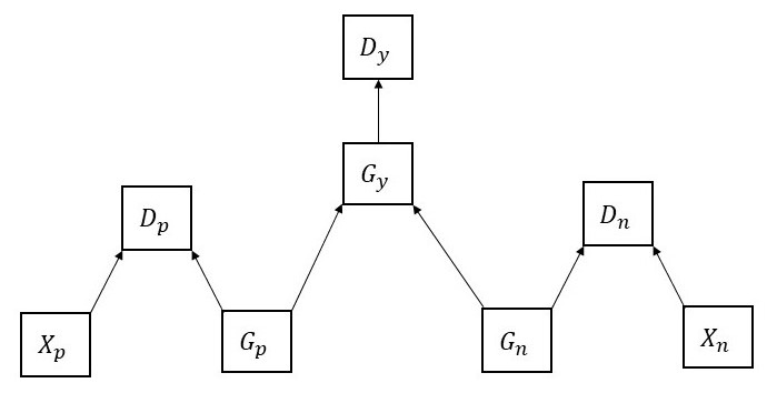
Figure 1: Schematic diagram of proposed model

This model uses three generators $(G_{p},G_{n},G_{y})$ and three discriminators $(D_{p},D_{n},D_{y})$. $G_{p}$ is responsible for generating positive claims and $Dp$ discriminates between original positive claims and synthetically generated positive claims. $G_{n}$ and $D_{n}$ are responsible for similar functions for negative claims. $Gy$ and $Dy$ get the input from the data generated by $G_{p}$ and $G_{n}$ and generate a class label (0/1) and the $D_{y}$ is the discriminator for $G_{y}$.

2 Proposed Methodology

In the proposed methodology three GAN units are used. These three units are responsible for generating positive samples Equation 1, negative samples Equation 2 and class labels Equation 3. Algorithm 1 gives the steps to train the generators and discriminators.

$$\min_{G_{p}}\max_{D_{p}}V(D,G)=\mathop{\mathbb{E}_{x\sim p_{p}{(x)}}}log(D_{p}(x))+\mathop{\mathbb{E}_{z\sim p_{z}{(z)}}}log(1-D_{p}(G_{p}(z)))$$ (1)

$$\min_{G_{n}}\max_{D_{n}}V(D,G)=\mathop{\mathbb{E}_{x\sim p_{n}{(x)}}}log(D_{n}(x))+\mathop{\mathbb{E}_{z\sim p_{z}{(z)}}}log(1-D_{n}(G_{n}(z)))$$ (2)

$$\begin{split}\min_{G_{p},G_{n},G_{y}}\max_{D_{y}}V(D,G)=\mathop{\mathbb{E}_{x\sim p{(x)}}}log(D_{y}(x))+\pi_{p}\mathop{\mathbb{E}_{z\sim p_{z}{(z)}}}log(1-D_{y}(G_{y}(G_{p}(z))))+\\ \pi_{n}\mathop{\mathbb{E}_{z\sim p_{z}{(z)}}}log(1-D_{y}(G_{y}(G_{n}(z))))\end{split}$$ (3)

Algorithm 1 Algorithm

1:

2:for training iterations do

3:     # update discriminator networks $D_{p},D_{n},D_{y}$ #

4:     sample mini-batch of noise examples $\{z^{i}\}^{m}_{i=1}$ from noise prior $p_{z}(z)$

5:     sample mini-batch of positive examples $\{x_{p}\}^{m}_{i=1}$ from noise prior $p_{p}(x)$

6:     sample mini-batch of negative examples $\{x_{n}\}^{m}_{i=1}$ from noise prior $p_{n}(x)$

7:     sample mini-batch of examples $\{x\}^{m}_{i=1}$ from noise prior $p(x)$

8:     update the positive discriminator $D_{p}$ by ascending its stochastic gradient:$\nabla_{\theta_{D_{p}}}\frac{1}{m}\sum_{i=1}^{m}\pi_{p}[log(D_{p}(x^{i}_{p}))+log(1-D_{p}(G_{p}(z^{i})))]$

9:     update the negative discriminator $D_{n}$ by ascending its stochastic gradient:$\nabla_{\theta_{D_{n}}}\frac{1}{m}\sum_{i=1}^{m}\pi_{n}[log(D_{n}(x^{i}_{n}))+log(1-D_{n}(G_{n}(z^{i})))]$

10:     update the discriminator $D_{y}$ by ascending its stochastic gradient:$\nabla_{\theta_{D_{y}}}\frac{1}{m}\sum_{i=1}^{m}\pi_{p}[log(D_{y}(x^{i}))+\pi_{p}log(1-D_{y}(G_{y}(G_{p}(z)))+\pi_{n}log(1-D_{y}(G_{y}(G_{n}(z)))]$

11:     # update generator networks $G_{p},G_{n},G_{y}$ #

12:     sample mini-batch of noise examples $\{z^{i}\}^{m}_{i=1}$from noise prior $p(z)$

13:     update the positive generator $G_{p}$ by descending its stochastic gradient: $\nabla_{\theta_{G_{p}}}\frac{1}{m}\sum_{i=1}^{m}\pi_{p}[-log(D_{p}(G_{p}(z^{i}))-log(D_{y}(G_{p}(z^{i}))]$

14:     update the negative generator $G_{p}$ by descending its stochastic gradient: $\nabla_{\theta_{G_{n}}}\frac{1}{m}\sum_{i=1}^{m}\pi_{n}[-log(D_{n}(G_{n}(z^{i}))-log(D_{y}(G_{n}(z^{i}))]$

15:     update the class label generator $G_{y}$ by descending its stochastic gradient: $\nabla_{\theta_{G_{y}}}\frac{1}{m}\sum_{i=1}^{m}[-\pi_{p}log(D_{y}(G_{p}(z^{i}))-\pi_{n}log(D_{y}(G_{n}(z^{i}))]$

16:end for

17:return $G_{y}$

The proposed model can handle only supported and refuted claims. $D_{y}$ will be trained with both supported and refuted claims, while $D_{p}$ and $D_{n}$ will be trained with only supported and refuted claims separately hence, $D_{y}$ is a more powerful discriminator compared to $D_{p}$ and $D_{n}$. There is a possibility that $D_{p}$ or $D_{n}$ will assign some sentences generated by $G_{p}$ and $G_{n}$ wrongly. As $D_{y}$ has the global view of both supported and refuted claims, it is capable of classifying them. Consider a situation: $G_{p}$ generates $Y_{p}$ (a synthetic positive claim). In the next step, $Y_{p}$ is the input to $G_{y}$, and $G_{y}$ is generating 1 (positive class label). The output of $G_{y}$ and input of $G_{p}$ is the input to the discriminator state ($D_{y}$). If $D_{y}$ classifies the $Y_{p}$ as positive, then there is no penalty that will be added to $G_{y}$ and $G_{p}$ otherwise penalties will be added to both $G_{p}$ and $G_{y}$. Consider another situation, where the $G_{y}$ generates 0 (negative class label) for an input of $Y_{p}$ and $D_{y}$ is also classifies the $Y_{p}$ as negative, then a penalty will be added to $G_{p}$, not $G_{y}$. So $D_{y}$ is acting as a global discriminator. Equation 4 is the loss function for the generator $G_{y}$. $\pi_{p}$ and $\pi_{n}$ are the probabilities of positive and negative claims in the dataset.

$$\begin{split}L(y)=\pi_{p}[D_{y}(G_{p}(z))log(D_{y}(G_{y}(G_{p}(z))))+(1-D_{y}(G_{p}(z)))log(1-D_{y}(G_{p}(z)))]+\\ \pi_{n}[D_{y}(G_{n}(z))log(D_{y}(G_{y}(G_{n}(z))))+(1-D_{y}(G_{n}(z)))log(1-D_{y}(G_{n}(z)))]\end{split}$$ (4)

For a GAN system achieving the equilibrium condition is very important. In the present context, to find the equilibrium condition, first, we need to find the optimal conditions for discriminators. Using the optimal conditions of the discriminators, the minimization conditions for the generator can be obtained. Considering the generators ($G_{p}$, $G_{n}$, $G_{y}$) are fixed, and $\pi_{p}$ and $\pi_{n}$ are the probabilities of positive and negative claims in the dataset. So in the in equilibrium condition the distribution of positive generated data ($p_{gp}(x)$) and negative generated data ($p_{gn}(x)$) will follow the below mentioned Equations 5 and 6. In Equations 5 and 6, $p_{p}(x)$ and $p_{n}(x)$ are the positive and negative class probability distributions.

$$p_{gp}(x)=p_{p}(x)$$ (5)

$$p_{gn}(x)=p_{n}(x)$$ (6)

The optimal discriminator functions $D_{p}^{*}(x)$, $D_{n}^{*}(x)$, $D_{y}^{*}(x)$ can be derived by differentiate Equation 1, 2 and 3.

$$D^{*}_{P}(x)=\frac{p_{p}(x)}{p_{p}(x)+p_{gp}(x)}$$ (7)

$$D^{*}_{n}(x)=\frac{p_{n}(x)}{p_{n}(x)+p_{gn}(x)}$$ (8)

$$\begin{split}\min_{G_{p},G_{n},G_{y}}\max_{D_{y}}V(D^{*},G)=log\left(\frac{p(x)}{p(x)+\pi_{p}p_{gp}(x)+\pi_{n}p_{gn}(x)}\right)+\\ \pi_{p}log\left(\frac{\pi_{p}p_{gp}(x)+\pi_{n}p_{gn}(x)}{p(x)+\pi_{p}p_{gp}(x)+\pi_{n}p_{gn}(x)}\right)+\\ \pi_{n}log\left(\frac{\pi_{p}p_{gp}(x)+\pi_{n}p_{gn}(x)}{p(x)+\pi_{p}p_{gp}(x)+\pi_{n}p_{gn}(x)}\right)\end{split}$$ (9)

Using Jensen–Shannon divergence (JSD) [7], we can show that the minimum value of the generators can be achieved when following conditions will be satisfied:

$$p_{p}(x)=p_{gp}(x)$$ (10)

$$p_{n}(x)=p_{gn}(x)$$ (11)

$$p_{y}(x)=\pi_{p}p_{gp}(x)+\pi_{n}p_{gn}(x)$$ (12)

The derivation steps of the above mentioned equations is presented in Appendix A.

3 Data

FEVER dataset is used for this research. It is a publicly available dataset for claim verification. There are three types of claims present in the dataset i) supported, ii) refuted, iii) information not enough (INE). For every supported and refuted claim there is one or multiple supporting evidence, while for the INE class there is no evidence. All evidence provided in the FEVER dataset is collected from Wikipedia. In most cases, the first few lines of a particular Wikipedia page are taken in FEVER dataset as the evidence. In Table 1 two examples of the claim, evidence and class label are presented.

Table 1: Examples of claim verification

Claim: Tetris has sold millions of physical copies.

Evidence: It was announced that Tetris has sold more than 170 million

copies, approximately 70 physical copies and …

Label: True

Claim: Andy Roddick lost 5 Master Series between 2002 and 2010.

Evidence: Roddick was ranked in the top 10 for nine consecutive years

between 2002 and 2010, and

won five Masters Series in that period.

Label: False

FEVER training dataset has 80,035 Supported claims, 29,775 Refuted claims, and 35,639 NotEnoughInfo claims. The FEVER 1.0 validation set and test set have 3,333 Support claims, 3,333 Refute claims, and 3,333 NotEnoughInfo claims respectively. FEVER 2.0 has 391 Support claims, 396 Refute claims, and 387 NotEnoughInfo claims respectively. For the experiments we used only supported and refuted claims.

4 Experiments

The algorithm described in the previous section is implemented and tested using the FEVER 1.0 and FEVER 2.0 datasets. The steps of the experiments are described in this section.

4.1 Data preprocessing:

For this experiment, only ‘Supported’ and ‘Refuted’ claims are considered from the training dataset. In the training dataset, every claim has one or multiple evidence. For a particular claim, its corresponding evidence is concatenated separately. For example, there is a data point with the following claim $(C)$ evidence $(E)$ and label $(L):[C,E<e_{1},e_{2},e_{3}>,L].$ The input data format for the further processes will be: $x=[<C;e_{1},L>,<C;e_{2},L>,<C;e_{3},L>]$. This preprocessed claim evidence pair is used for further experiments.

4.2 GAN Implementation:

The implementation of GAN is the central part of this research. There are two types of GAN implemented: text generating GAN and binary class label generating GAN. The text generating GAN is generating synthetic text data for supported and refuted claims. The binary class label generating GAN generates the binary class label for each of the generated claims. To implement text generating GAN, we followed LaTextGAN [4]. LaTextGAN follows two phases for the implementation. During the first phase, it creates an encoded space, and in the second phase, it follows the traditional GAN [10] implementation steps and generates synthetic data in the encoded space. Finally, the synthetically generated data is decoded into normal text data. On the other hand, the implementation of binary labels generating GAN is similar to the implementation of the traditional GAN [10].

4.3 GenPU Based Methods:

The proposed model is inspired by the GenPU. To explore further we have modified GenPU in two variants such as Inverted GenPU and Symmetric GenPU. In case of Inverted GenPU the value functions for the positive and negative text generating GAN are exchanged. Hence the respective value functions become the equations mentioned in Equation 13, 14 and 15.

$$D^{*}_{n}=\operatorname*{argmax}_{D_{n}}\mathop{\mathbb{E}_{x\sim p_{p}{(x)}}}log(D_{n}(x))+\mathop{\mathbb{E}_{z\sim p_{z}{(z)}}}log(1-D_{u}(G_{n}(z)))$$ (13)

$$\min_{G_{p}}\max_{D_{p}}V(D,G)=-\mathop{\mathbb{E}_{x\sim p_{p}{(x)}}}log(D^{*}_{n}(x))-\mathop{\mathbb{E}_{z\sim p_{z}{(z)}}}log(1-D^{*}_{n}(G_{n}(z)))$$ (14)

$$\min_{G_{n}}\max_{D_{n}}V(D,G)=\mathop{\mathbb{E}_{x\sim p_{p}{(x)}}}log(D_{p}(x))+\mathop{\mathbb{E}_{z\sim p_{z}{(z)}}}log(1-D_{p}(G_{p}(z)))$$ (15)

In Symmetric GenPU the equations for both the value functions are same. The value functions for Symmetric GenPU are presented in Equation 16 and 17.

$$\min_{G_{p}}\max_{D_{p}}V(D,G)=\mathop{\mathbb{E}_{x\sim p_{p}{(x)}}}log(D_{p}(x))+\mathop{\mathbb{E}_{z\sim p_{z}{(z)}}}log(1-D_{p}(G_{p}(z)))$$ (16)

$$\min_{G_{n}}\max_{D_{n}}V(D,G)=\mathop{\mathbb{E}_{x\sim p_{p}{(x)}}}log(D_{p}(x))+\mathop{\mathbb{E}_{z\sim p_{z}{(z)}}}log(1-D_{p}(G_{p}(z)))$$ (17)

4.4 Other methods:

The performance of the proposed method is compared with other GAN based methods and classifiers. The GAN based models generate synthetic data and the synthetically generated data is added to the original dataset and it helps to create an extended feature space of the FEVER dataset and gives leverage to new features. This synthetically generated data is further classified using positive-unlabeled (PU) learning which considers supported facts as positive class and are added to the existing training dataset. Finally, this extended dataset is used for the training process. The synthetic data is generated using LeakGAN [11] and LaTextGAN [4] separately and two different sets of results are collected to compare the performance. Other than GAN based methods different deep learning and machine learning based classification methods are used such as: BERT based classifier [3], Graph Convolution Network (GCN) [31], Long Short Term Memory (LSTM) [12], Convolution Neural Network (CNN) [15], Support Vector Machine (SVM) [5], Naive Bayes [16], Random forest [20], Stochastic Gradient Descent (SGD) [6] are also implemented for the claim verification task. To implement BERT based classifier Huggingface BERT [3] pretrained transformer is used as tokenizer for the training, validation and testing dataset. The vocabulary size of the pretrained model is 30522 and the size of the hidden layer is 768. Later the pretuned model is fine tuned to classify the claims. In GCN, the point wise mutual information between words is calculated to generate the graph. To implement the CNN five kernels of sizes 2, 3, 4, 5 and 6 are used. For LSTM the input data is encoded using GloVe [25]. The learning rate and batch size for GCN, CCN and LSTM are 0.001, 64 respectively. The Random forest is equipped with 1000 trees and entropy is used as supported criteria for the information gain. The SGB model utilizes hinge loss and L2 penalty. The deep learning models are implemented using PyTorch [22], and the Scikit learn library [23] is used for machine learning models.

5 Results

In this section the results of the previously discussed experiments will be discussed. All models are trained with the FEVER training dataset and tested with FEVER 1.0 and FEVER 2.0 test dataset. In the Table 2 and Table 3 detailed results for each of the models are presented. Each of the experiments is repeated five times. The result for FEVER 1.0 is also compared with previous research work by Yang et al. [39].

Table 2: Result of FEVER 1.0

	FEVER 1.0 Dataset
Classifiers	Precision	Recall	F1 Score
BERT Classifier	0.45 $\pm$ 0.011	0.44 $\pm$ 0.010	0.44 $\pm$ 0.009
Leak GAN Based Classifier	0.65 $\pm$ 0.003	0.64 $\pm$ 0.006	0.63 $\pm$ 0.003
LaTextGAN Based Classifier	0.41 $\pm$ 0.008	0.36 $\pm$ 0.016	0.30 $\pm$ 0.009
Graph Convolutional Network	0.45 $\pm$ 0.015	0.44 $\pm$ 0.013	0.44 $\pm$ 0.013
SVM	0.53 $\pm$ 0.013	0.42 $\pm$ 0.013	0.38 $\pm$ 0.013
Naive Bayes	0.41 $\pm$ 0.016	0.34 $\pm$ 0.014	0.24 $\pm$ 0.015
Random forest	0.33 $\pm$ 0.011	0.33 $\pm$ 0.010	0.28 $\pm$ 0.011
SGD	0.31 $\pm$ 0.023	0.22 $\pm$ 0.022	0.27 $\pm$ 0.023
LSTM	0.45 $\pm$ 0.003	0.42 $\pm$ 0.004	0.004 $\pm$ 0.004
CNN	0.46 $\pm$ 0.012	0.44 $\pm$ 0.011	0.43 $\pm$ 0.012
Inverted GenPU	0.52 $\pm$ 0.013	0.71 $\pm$ 0.023	0.60 $\pm$ 0.018
Symmetric GenPU	0.33 $\pm$ 0.015	0.54 $\pm$ 0.02	0.40 $\pm$ 0.016
Proposed Method	0.50 $\pm$ 0.016	0.93 $\pm$ 0.018	0.65 $\pm$ 0.018
Yang et al. result	0.61	0.58	0.60

In Table 2 and Table 3 it can be observed that the F1 score for the proposed method is better than the rest of the models and the previous research.

The proposed GAN model has three generator-discriminator pairs and each of them is having one loss function. To generate very good quality synthetic data, the loss should be minimized. While training the model we observed losses of three generator-discriminator pairs such as positive loss, negative loss and binary label loss. In the Fig. 4, Fig. 5 and Fig. 8 it can be observed that the loss of three generator-discriminator pairs is gradually reduced.

Table 3: Result of FEVER 2.0

	FEVER 2.0 Dataset
Classifiers	Precision	Recall	F1 Score
BERT Classifier	0.46 $\pm$ 0.013	0.44 $\pm$ 0.014	0.44 $\pm$ 0.013
Leak GAN Based Classifier	0.52 $\pm$ 0.023	0.51 $\pm$ 0.019	0.51 $\pm$ 0.021
LaTextGAN Based Classifier	0.42 $\pm$ 0.02	0.39 $\pm$ 0.019	0.39 $\pm$ 0.019
Graph Convolutional Network	0.43 $\pm$ 0.023	0.39 $\pm$ 0.013	0.37 $\pm$ 0.016
SVM	0.40 $\pm$ 0.019	0.37 $\pm$ 0.022	0.35 $\pm$ 0.019
Naive Bayes	0.33 $\pm$ 0.030	0.22 $\pm$ 0.023	0.27 $\pm$ 0.025
Random forest	0.33 $\pm$ 0.014	0.26 $\pm$ 0.017	0.29 $\pm$ 0.015
SGD	0.30 $\pm$ 0.025	0.22 $\pm$ 0.029	0.26 $\pm$ 0.027
LSTM	0.43 $\pm$ 0.028	0.40 $\pm$ 0.039	0.39 $\pm$ 0.032
CNN	0.41 $\pm$ 0.021	0.38 $\pm$ 0.011	0.37 $\pm$ 0.018
Inverted GenPU	0.58 $\pm$ 0.024	0.71 $\pm$ 0.022	0.63 $\pm$ 0.012
Symmetric GenPU	0.41 $\pm$ 0.016	0.55 $\pm$ 0.011	0.49 $\pm$ 0.013
Proposed Method	0.49 $\pm$ 0.061	0.97 $\pm$ 0.041	0.65 $\pm$ 0.051

The proposed GAN based model starts with some random values and tries to generate synthetic data, which helps to achieve a better F1 score. In the training process, after every epoch, we have calculated the F1 score for both the test datasets and observed a gradual improvement of the F1 score. The gradual change of precision, recall, and F1 score for the FEVER 1.0 and FEVER 2.0 is presented in Fig. 3 and Fig. 3. Moreover, to visualize the distribution of original and synthetically data, the t-SNE plot of the positive and negative generated data is shown in Fig. 4 and Fig. 5. The perplexity of the t-SNE plot is 30, and the learning rate is 120. It can be observed that the distribution of synthetically generated positive data is very similar to that of original positive text data, while the distribution of the negative synthetic data is similar to the original negative text data. The positive synthetic data is much more similar to the positive text data compared to the similarity between negative synthetic data and negative text data.

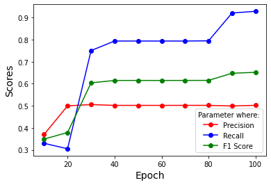
Figure 2: Precision, Recall and F1 Score for FEVER 1.0 Dataset

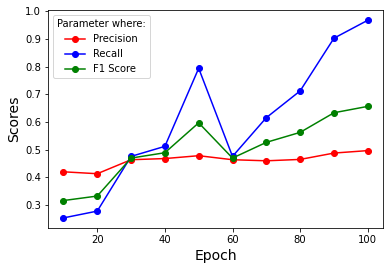
Figure 3: Precision, Recall and F1 Score for FEVER 2.0 Dataset

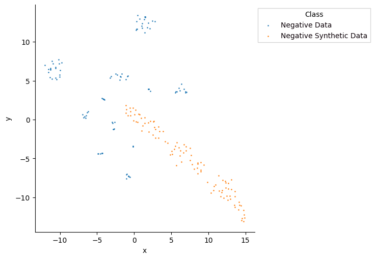
(a) Epoch = 25

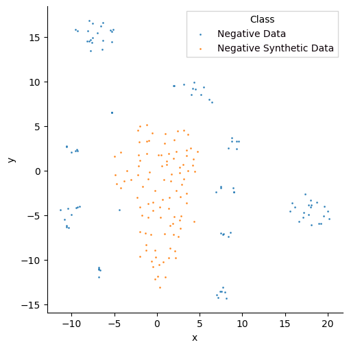
(b) Epoch = 50

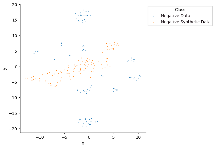
(c) Epoch = 75

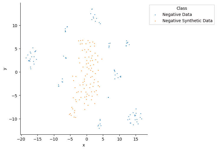
(d) Epoch = 100

Figure 4: t-SNE Plot of original and synthetic data for negative class

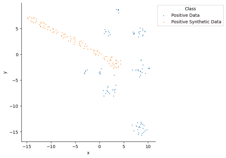
(a) Epoch = 25

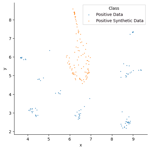
(b) Epoch = 50

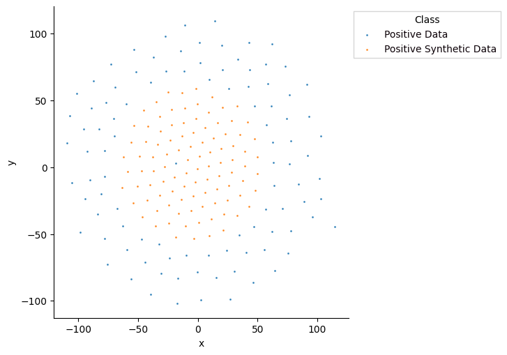
(c) Epoch = 75

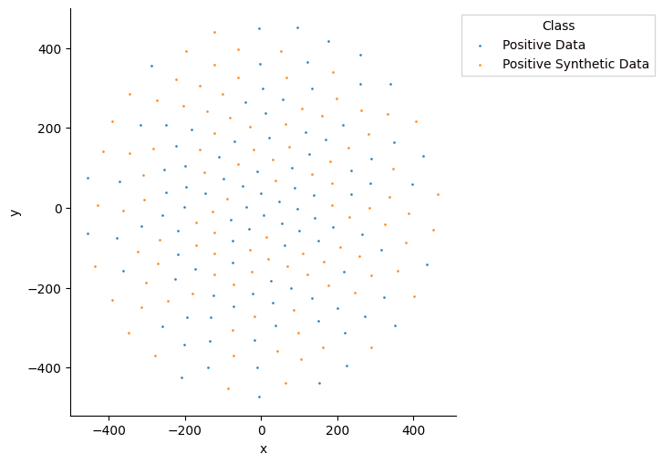
(d) Epoch = 100

Figure 5: t-SNE Plot of origianl and synthetic data for postive class

Fig. 8, 8, 8 depicting the positive loss, negative loss and label generating loss. We can see the three losses are decreasing over epochs gradually, which also suggests that all the generator discriminator pairs are training to achieve the equilibrium state. To test the gradual progression of the synthetically generated data, we also measure the similarity scores between original (positive and negative) data and synthetic data (positive and negative) while training the model. It has been observed that for the generated data, the similarity score gradually improves over epochs, as shown in Fig. 9 and 10. To measure the similarity 20,000 synthetically generated data are randomly selected and Cosine similarity [32], Manhattan distance [33], Euclidean distance [1] are calculated.

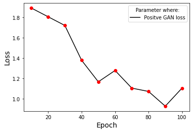
Figure 6: Postive loss

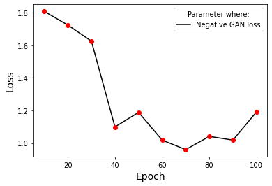
Figure 7: Negative loss

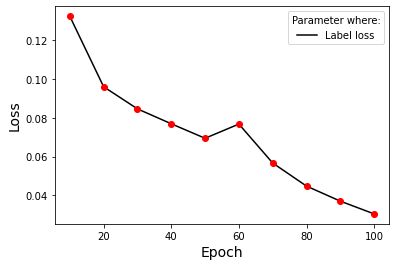
Figure 8: Label loss

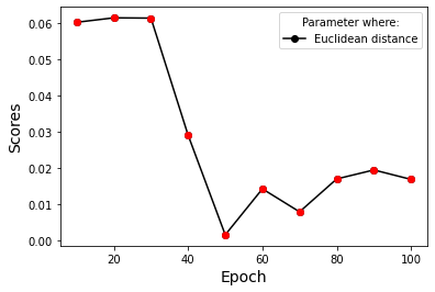
(a) Cosine distance

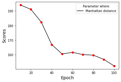
(b) Manhattan distance

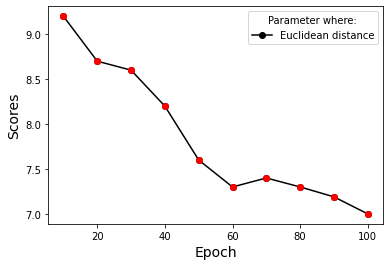
(c) Euclidean distance

Figure 9: Similarity scores for positive data

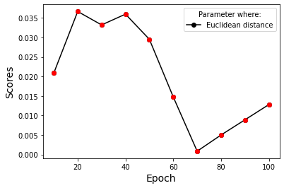
(a) Cosine distance

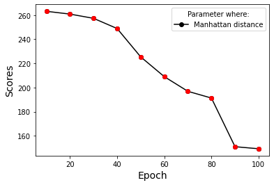
(b) Manhattan distance

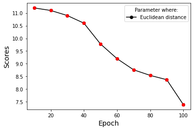
(c) Euclidean distance

Figure 10: Similarity scores for negative data

6 Conclusion

This research proposes a multiple GAN-based model that employs the GAN’s synthetic data generation capability to solve claim verification problems. The model generates synthetic data for supported, refuted claims and their class labels using three separate generator discriminator pairs. The synthetic data eventually helps in the fact-checking task for FEVER 1.0 and FEVER 2.0 test datasets. The results have shown that the proposed model starts with random data generation, and as the training progresses, it generates synthetic data similar to the original data. Different statistical and analytical similarity metrics confirm that the similarity between original data and synthetically generated data increases as the training progresses. This gradual improvement of data quality shows the effectiveness of the model. The proposed model produces an F1 score of 0.65 $\pm$ 0.018 and 0.65 $\pm$ 0.051 for FEVER 1.0 and FEVER 2.0, respectively. In the future, this model can be extended to a multi-class classifier, and a similar set of experiments can be carried out on other publicly available standard datasets to test this proposed model’s effectiveness.

Appendix A Mathematical Calculations

In the proposed methodology three GAN units are used. These three units are responsible for generating positive samples Equation 18, negative samples Equation 19 and class labels Equation 20.

$$\min_{G_{p}}\max_{D_{p}}V(D,G)=\mathop{\mathbb{E}_{x\sim p_{p}{(x)}}}log(D_{p}(x))+\mathop{\mathbb{E}_{z\sim p_{z}{(z)}}}log(1-D_{p}(G_{p}(z)))$$ (18)

$$\min_{G_{n}}\max_{D_{n}}V(D,G)=\mathop{\mathbb{E}_{x\sim p_{n}{(x)}}}log(D_{n}(x))+\mathop{\mathbb{E}_{z\sim p_{z}{(z)}}}log(1-D_{n}(G_{n}(z)))$$ (19)

$$\begin{split}\min_{G_{p},G_{n},G_{y}}\max_{D_{y}}V(D,G)=\mathop{\mathbb{E}_{x\sim p{(x)}}}log(D_{y}(x))+\pi_{p}\mathop{\mathbb{E}_{z\sim p_{z}{(z)}}}log(1-D_{y}(G_{y}(G_{p}(z))))+\\ \pi_{n}\mathop{\mathbb{E}_{z\sim p_{z}{(z)}}}log(1-D_{y}(G_{y}(G_{n}(z))))\end{split}$$ (20)

To find the equilibrium condition, first, we need to find the optimal conditions for discriminators. Using the optimal conditions of the discriminators, the minimization conditions for the generator can be obtained. Considering the generators ($G_{p}$, $G_{n}$, $G_{y}$) are fixed, and $\pi_{p}$ and $\pi_{n}$ are the probabilities of positive and negative claims in the dataset. So in the in equilibrium condition the distribution of positive generated data ($p_{gp}(x)$) and negative generated data ($p_{gn}(x)$) will follow the below mentioned Equations 21 and 22.

$$p_{gp}(x)=p_{p}(x)$$ (21)

$$p_{gn}(x)=p_{n}(x)$$ (22)

To find the optimal discriminator functions $D_{p}^{*}(x)$, $D_{n}^{*}(x)$, $D_{y}^{*}(x)$ we need to differentiate Equation 18, 19 and 20.

Let, $a=\mathop{\mathbb{E}_{x\sim p_{p}{(x)}}}$, $b=\mathop{\mathbb{E}_{z\sim p_{p}{(z)}}}$ and $t=D_{p}(x)$. Substitution $a$, $b$ and $x$ in Equation 18 we get Equation 23.

$$l=a*log(t)+b*log(1-t)$$ (23)

Differentiating Equation 23 with respect to $t$ and equating the result with zero we can get the optimum value of $t$.

$$\diff{l}{t}=\frac{a}{t}-\frac{b}{(1-t)}=0$$ (24)

$$\frac{a}{t}=\frac{b}{(1-t)}$$ (25)

$$t=\frac{a}{(a+b)}$$ (26)

Therefore, substitution values of $a$ and $b$ the optimal discriminator function will be Equation 27. The value of $b$ is $p_{gp}$ for the optimum condition as discussed earlier.

$$D^{*}_{P}(x)=\frac{p_{p}(x)}{p_{p}(x)+p_{gp}(x)}$$ (27)

Similarly, we can derive the equation for the negative discriminator as shown in Equation 28.

$$D^{*}_{n}(x)=\frac{p_{n}(x)}{p_{n}(x)+p_{gn}(x)}$$ (28)

To find the optimal values discriminator function for $D_{y}$ we need to differentiate Equation 20.

Let, $a=\mathop{\mathbb{E}_{x\sim p_{p}{(x)}}}$, $b=\pi_{p}*\mathop{\mathbb{E}_{z\sim p_{p}{(z)}}}$, $c=\pi_{n}*\mathop{\mathbb{E}_{z\sim p_{p}{(z)}}}$ and $t=D_{y}(x)$. Substitution $a$, $b$, $c$ and $x$ in Equation 20 we get Equation 29.

$$l=a*log(t)+b*log(1-t)+c*log(1-t)$$ (29)

Differentiating Equation 29 with respect to $t$ and equating the result with zero we can get the optimum value of $t$.

$$\diff{l}{t}=\frac{a}{t}+\frac{b}{1-t}+\frac{c}{1-t}=0$$ (30)

$$t=\frac{a}{a+b+c}$$ (31)

Substituting the values of $a,b,c$ gives the Equation 32.

$$\begin{split}\min_{G_{p},G_{n},G_{y}}\max_{D_{y}}V(D^{*},G)=log\left(\frac{p(x)}{p(x)+\pi_{p}p_{gp}(x)+\pi_{n}p_{gn}(x)}\right)+\\ \pi_{p}log\left(\frac{\pi_{p}p_{gp}(x)+\pi_{n}p_{gn}(x)}{p(x)+\pi_{p}p_{gp}(x)+\pi_{n}p_{gn}(x)}\right)+\\ \pi_{n}log\left(\frac{\pi_{p}p_{gp}(x)+\pi_{n}p_{gn}(x)}{p(x)+\pi_{p}p_{gp}(x)+\pi_{n}p_{gn}(x)}\right)\end{split}$$ (32)

Using Jensen–Shannon divergence (JSD) [7], we can show that the minimum value of the generators can be achieved when following conditions will be satisfied:

$$p_{p}(x)=p_{gp}(x)$$ (33)

$$p_{n}(x)=p_{gn}(x)$$ (34)

$$p_{y}(x)=\pi_{p}p_{gp}(x)+\pi_{n}p_{gn}(x)$$ (35)

References

[1]
Charu C Aggarwal, Alexander Hinneburg, and Daniel A Keim.
On the surprising behavior of distance metrics in high dimensional
space.
pages 420–434, 2001.
[2]
Ramy Baly, Georgi Karadzhov, Dimitar Alexandrov, James Glass, and Preslav
Nakov.
Predicting factuality of reporting and bias of news media sources.
arXiv preprint arXiv:1810.01765, 2018.
[3]
Jacob Devlin, Ming-Wei Chang, Kenton Lee, and Kristina Toutanova.
Bert: Pre-training of deep bidirectional transformers for language
understanding.
arXiv preprint arXiv:1810.04805, 2018.
[4]
David Donahue and Anna Rumshisky.
Adversarial text generation without reinforcement learning.
arXiv preprint arXiv:1810.06640, 2018.
[5]
Harris Drucker, Christopher J Burges, Linda Kaufman, Alex Smola, and Vladimir
Vapnik.
Support vector regression machines.
Advances in neural information processing systems, 9:155–161,
1996.
[6]
Jerome H Friedman.
Stochastic gradient boosting.
Computational statistics & data analysis, 38(4):367–378,
2002.
[7]
Bent Fuglede and Flemming Topsoe.
Jensen-shannon divergence and hilbert space embedding.
page 31, 2004.
[8]
Matt Gardner, Joel Grus, Mark Neumann, Oyvind Tafjord, Pradeep Dasigi,
Nelson F. Liu, Matthew Peters, Michael Schmitz, and Luke S. Zettlemoyer.
Allennlp: A deep semantic natural language processing platform.
2017.
arXiv:arXiv:1803.07640.
[9]
Liang Ge, Jing Gao, Xiaoyi Li, and Aidong Zhang.
Multi-source deep learning for information trustworthiness
estimation.
pages 766–774, 2013.
[10]
Ian Goodfellow, Jean Pouget-Abadie, Mehdi Mirza, Bing Xu, David Warde-Farley,
Sherjil Ozair, Aaron Courville, and Yoshua Bengio.
Generative adversarial nets.
Advances in neural information processing systems,
27:2672–2680, 2014.
[11]
Jiaxian Guo, Sidi Lu, Han Cai, Weinan Zhang, Yong Yu, and Jun Wang.
Long text generation via adversarial training with leaked
information.
arXiv preprint arXiv:1709.08624, 2017.
[12]
Sepp Hochreiter and Jürgen Schmidhuber.
Long short-term memory.
Neural computation, 9(8):1735–1780, 1997.
[13]
Ming Hou, Brahim Chaib-Draa, Chao Li, and Qibin Zhao.
Generative adversarial positive-unlabelled learning.
arXiv preprint arXiv:1711.08054, 2017.
[14]
Klaus Krippendorff.
Content analysis: An introduction to its methodology.
2018.
[15]
Steve Lawrence, C Lee Giles, Ah Chung Tsoi, and Andrew D Back.
Face recognition: A convolutional neural-network approach.
IEEE transactions on neural networks, 8(1):98–113, 1997.
[16]
David D Lewis.
Naive (bayes) at forty: The independence assumption in information
retrieval.
pages 4–15, 1998.
[17]
Qi Li, Yaliang Li, Jing Gao, Bo Zhao, Wei Fan, and Jiawei Han.
Resolving conflicts in heterogeneous data by truth discovery and
source reliability estimation.
pages 1187–1198, 2014.
[18]
Rada Mihalcea and Carlo Strapparava.
The lie detector: Explorations in the automatic recognition of
deceptive language.
pages 309–312, 2009.
[19]
Kimberly A Neuendorf and Anup Kumar.
Content analysis.
The international encyclopedia of political communication,
pages 1–10, 2015.
[20]
Mahesh Pal.
Random forest classifier for remote sensing classification.
International journal of remote sensing, 26(1):217–222, 2005.
[21]
Jeff Pasternack and Dan Roth.
Making better informed trust decisions with generalized fact-finding.
2011.
[22]
Adam Paszke, Sam Gross, Francisco Massa, Adam Lerer, James Bradbury, Gregory
Chanan, Trevor Killeen, Zeming Lin, Natalia Gimelshein, Luca Antiga, Alban
Desmaison, Andreas Kopf, Edward Yang, Zachary DeVito, Martin Raison, Alykhan
Tejani, Sasank Chilamkurthy, Benoit Steiner, Lu Fang, Junjie Bai, and Soumith
Chintala.
Pytorch: An imperative style, high-performance deep learning library.
pages 8024–8035, 2019.
URL:
http://papers.neurips.cc/paper/9015-pytorch-an-imperative-style-high-performance-deep-learning-library.pdf.
[23]
F. Pedregosa, G. Varoquaux, A. Gramfort, V. Michel, B. Thirion, O. Grisel,
M. Blondel, P. Prettenhofer, R. Weiss, V. Dubourg, J. Vanderplas, A. Passos,
D. Cournapeau, M. Brucher, M. Perrot, and E. Duchesnay.
Scikit-learn: Machine learning in Python.
Journal of Machine Learning Research, 12:2825–2830, 2011.
[24]
James W Pennebaker, Martha E Francis, and Roger J Booth.
Linguistic inquiry and word count: Liwc 2001.
Mahway: Lawrence Erlbaum Associates, 71(2001):2001, 2001.
[25]
Jeffrey Pennington, Richard Socher, and Christopher D Manning.
Glove: Global vectors for word representation.
pages 1532–1543, 2014.
[26]
Verónica Pérez-Rosas, Bennett Kleinberg, Alexandra Lefevre, and Rada
Mihalcea.
Automatic detection of fake news.
arXiv preprint arXiv:1708.07104, 2017.
[27]
Ravali Pochampally, Anish Das Sarma, Xin Luna Dong, Alexandra Meliou, and
Divesh Srivastava.
Fusing data with correlations.
pages 433–444, 2014.
[28]
Kashyap Popat, Subhabrata Mukherjee, Andrew Yates, and Gerhard Weikum.
Declare: Debunking fake news and false claims using evidence-aware
deep learning.
arXiv preprint arXiv:1809.06416, 2018.
[29]
Hannah Rashkin, Eunsol Choi, Jin Yea Jang, Svitlana Volkova, and Yejin Choi.
Truth of varying shades: Analyzing language in fake news and
political fact-checking.
pages 2931–2937, 2017.
[30]
Victoria L Rubin, Yimin Chen, and Nadia K Conroy.
Deception detection for news: three types of fakes.
Proceedings of the Association for Information Science and
Technology, 52(1):1–4, 2015.
[31]
Franco Scarselli, Marco Gori, Ah Chung Tsoi, Markus Hagenbuchner, and Gabriele
Monfardini.
The graph neural network model.
IEEE Transactions on Neural Networks, 20(1):61–80, 2008.
[32]
Amit Singhal et al.
Modern information retrieval: A brief overview.
IEEE Data Eng. Bull., 24(4):35–43, 2001.
[33]
Deepak Sinwar and Rahul Kaushik.
Study of euclidean and manhattan distance metrics using simple
k-means clustering.
Int. J. Res. Appl. Sci. Eng. Technol, 2(5):270–274, 2014.
[34]
James Thorne and Andreas Vlachos.
Adversarial attacks against fact extraction and verification.
arXiv preprint arXiv:1903.05543, 2019.
[35]
James Thorne, Andreas Vlachos, Christos Christodoulopoulos, and Arpit Mittal.
Fever: a large-scale dataset for fact extraction and verification.
arXiv preprint arXiv:1803.05355, 2018.
[36]
James Thorne, Andreas Vlachos, Oana Cocarascu, Christos Christodoulopoulos, and
Arpit Mittal.
The fact extraction and verification (fever) shared task.
arXiv preprint arXiv:1811.10971, 2018.
[37]
James Thorne, Andreas Vlachos, Oana Cocarascu, Christos Christodoulopoulos, and
Arpit Mittal.
The fever2. 0 shared task.
pages 1–6, 2019.
[38]
Mengting Wan, Xiangyu Chen, Lance Kaplan, Jiawei Han, Jing Gao, and Bo Zhao.
From truth discovery to trustworthy opinion discovery: An
uncertainty-aware quantitative modeling approach.
pages 1885–1894, 2016.
[39]
Fan Yang, Eduard Dragut, and Arjun Mukherjee.
Claim verification under positive unlabeled learning.
IEEE/ACM International Conference on Advances in Social Networks
Analysis and Mining (ASONAM), 2020.
[40]
Yang Yang, Lei Zheng, Jiawei Zhang, Qingcai Cui, Zhoujun Li, and Philip S Yu.
Ti-cnn: Convolutional neural networks for fake news detection.
arXiv preprint arXiv:1806.00749, 2018.