Flow views and infinite interval exchange transformations for recognizable substitutions

Abstract.

A flow view is the graph of a measurable conjugacy $\displaystyle\Phi$ between a substitution or S-adic subshift $\displaystyle({\Sigma},\operatorname{\sigma},\mu)$ and an exchange of infinitely many intervals in $\displaystyle([0,1],\mathfrak{F},m)$. The natural refining sequence of partitions of $\displaystyle{\Sigma}$ is transferred to $\displaystyle([0,1],m)$ using a canonical addressing scheme, a fixed dual substitution $\displaystyle{\mathcal{S}_{*}}$, and a shift-invariant probability measure $\displaystyle\mu$. On the flow view, $\displaystyle\boldsymbol{\tau}$ is shown horizontally at a height of $\displaystyle\Phi(\boldsymbol{\tau})$.

The IIET $\displaystyle\mathfrak{F}$ is well approximated by exchanges of finitely many intervals, making numeric and graphic methods possible. The graphs of $\displaystyle\mathfrak{F}$s show forms of self-similarity, a special case of which is proved. The spectral type of $\displaystyle\Phi\in L^{2}({\Sigma},\mu),$ is of particular interest. As an example of utility, some spectral results for constant-length substitutions are included.

1. Introduction

This paper shows how to construct an exchange transformation $\displaystyle\mathfrak{F}$ on infinitely many intervals in $\displaystyle[0,1]$ to represent any minimal and recognizable substitution subshift in $\displaystyle\mathbb{Z}$. (We say infinite interval exchange transformation or IIET for short). All probability measure preserving transformations are measurably conjugate to cut-and-stack transformations on $\displaystyle[0,1]$, so existence is not surprising [4]. Our construction provides several advantages:

Efficiency. All but $\displaystyle\epsilon$ of $\displaystyle[0,1]$ is contained in $\displaystyle\mathcal{O}(|\ln(\epsilon)|)$ intervals in the domain of $\displaystyle\mathfrak{F}$. We will show that for any $\displaystyle n\in\mathbb{N}$, there is an interval exchange tranformation $\displaystyle\mathfrak{F}_{n}$ that is equal to $\displaystyle\mathfrak{F}$ on $\displaystyle\mathcal{O}(n)$ intervals and differs on a set of measure $\displaystyle\leq\lambda^{-n}$. Figure 1 shows $\displaystyle\mathfrak{F}_{7}$ for the Fibonacci ($\displaystyle\alpha\to\alpha\beta,\,\beta\to\alpha$) and $\displaystyle\mathfrak{F}_{5}$ for Thue–Morse ($\displaystyle\alpha\to\alpha\beta,\,\beta\to\beta\alpha,$) substitutions. $\displaystyle\Diamond$

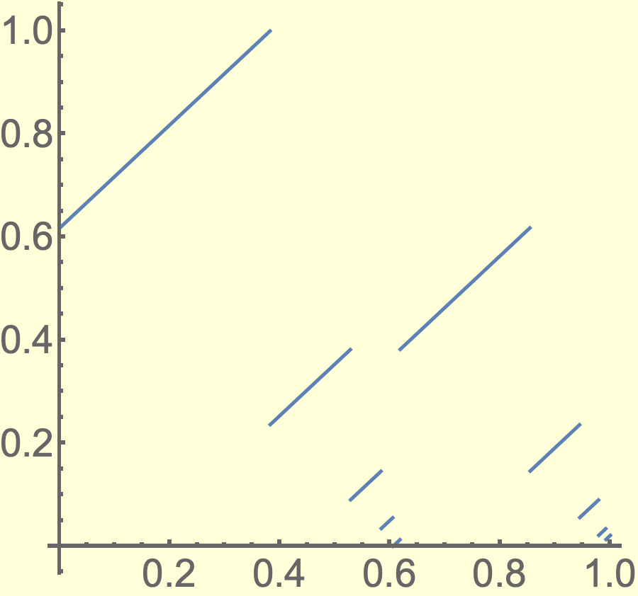
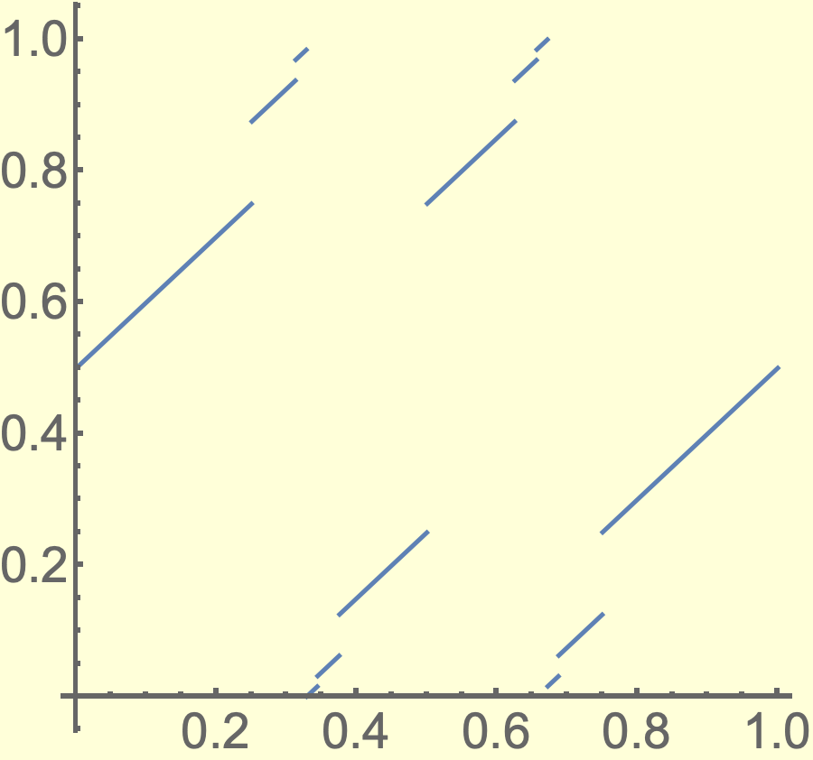
Figure 1. Canonical IIETs for Fibonacci (left) and Thue–Morse (right)

Visualization. The graph of the map $\displaystyle\Phi:{\Sigma}\to[0,1]$, called a flow view, is a picture of every sequence in $\displaystyle{\Sigma}$ lined up between $\displaystyle 0$ and $\displaystyle 1$. It literally graphs the a.e. one-to-one correspondence between $\displaystyle[0,1]$ and the subshift by showing each $\displaystyle\boldsymbol{\tau}\in{\Sigma}$ (in colored unit interval tiles) at a height of $\displaystyle\Phi(\boldsymbol{\tau})$. Figure 2 shows the central portion of the flow views for the Fibonacci and Thue–Morse substitutions. The vertical black line is the interval from 0 to 1 on the $\displaystyle y$-axis. $\displaystyle\Diamond$

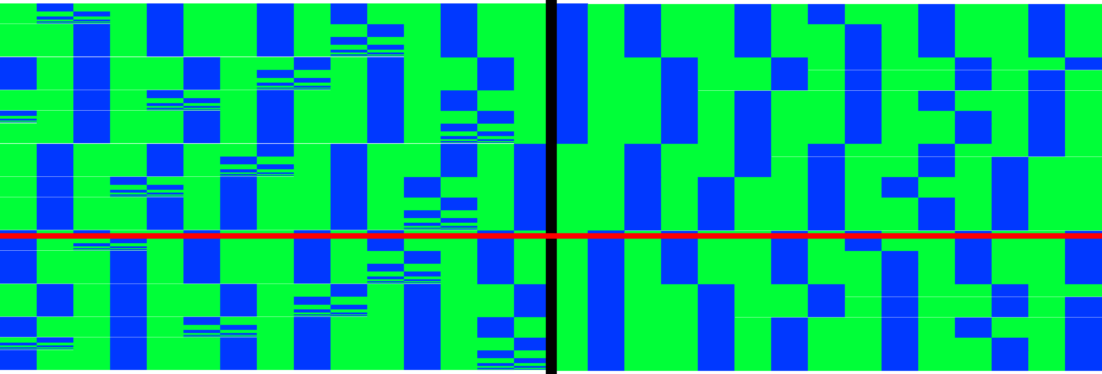
Figure 2. Flow views for Fibonacci (top) and Thue–Morse (bottom) subshifts. The red line highlights the $\displaystyle\boldsymbol{\tau}\in{\Sigma}$ for which $\displaystyle\Phi(\boldsymbol{\tau})={1}/{e}$

Generalizations. The construction works for a large class of S-adic systems and the adaptations necessary are provided. The continuous analogues, self-similar and fusion tilings of $\displaystyle\mathbb{R}$, are suspensions and therefore the results apply for a transversal. The construction works in some higher dimensional situations to produce commuting IIETs on $\displaystyle[0,1]$ and this work in ongoing [16]. $\displaystyle\Diamond$

Applications. The spectral theory of the subshift can be investigated in $\displaystyle L^{2}([0,1])$ directly. Moreover, $\displaystyle\Phi$ is a natural element of $\displaystyle L^{2}({\Sigma},\mu)$ whose spectral decomposition is particularly important. A few results are presented for constant-length substitutions to show the possibilities. Because of the intimate connection between translation surfaces and interval exchange transformations, our IIETs provide an unlimited stable of translation surfaces that are probably of infinite genus. The graphs of our IIETs show types of self-similarity properties, which is expected to simplify the basic analysis of their translation surfaces. $\displaystyle\Diamond$

There are three main ingredients in our construction. The first is a system for associating each $\displaystyle\boldsymbol{\tau}\in{\Sigma}$ with an address $\displaystyle{\boldsymbol{{\mathsf{a}}}}=({\mathsf{a}}_{1},{\mathsf{a}}_{2},...),$ where each $\displaystyle{\mathsf{a}}_{n}$ lives in a finite alphabet $\displaystyle\mathsf{A}$ that is different from the alphabet $\displaystyle{\mathcal{A}}$ of our substitution. This is closely related to a description of substitution subshifts via Bratteli diagrams, where $\displaystyle{\mathsf{a}}_{n}$ tells you which arrow to follow at level $\displaystyle n$. In our construction the label $\displaystyle{\mathsf{a}}_{n}$ represents how the $\displaystyle(n-1)$-supertile sits inside its $\displaystyle n$-supertile. The second ingredient is a function $\displaystyle{\phi}$ on the alphabet $\displaystyle\mathsf{A}$. This function is related to a choice of dual substitution, whose matrix is the transpose of the substitution matrix of our original, and to the left Perron-Frobenius eigenvector of that matrix. That vector is also a right Perron-Frobenius eigenvector of the original substitution matrix, so it represents frequencies in our original subshift. The third ingredient is a function $\displaystyle\Phi({\boldsymbol{{\mathsf{a}}}})=\Phi_{0}({\mathsf{a}}_{1})+\sum_{n=1}^{\infty}{\phi}({\mathsf{a}}_{n})\lambda^{-n}$, where $\displaystyle\lambda$ is the Perron-Frobenius eigenvalue and $\displaystyle\Phi_{0}({\mathsf{a}}_{1})$ depends on the letter at the origin. (This is remiscent of the Dumont-Thomas numeration scheme [6, 13].) This turns things inside-out. In the usual Bratteli diagram description, two tilings are in the same translational orbit only if they addresses have the same tail, and their relative displacement is given by a finite sum of the digits where they are different, where $\displaystyle{\mathsf{a}}_{1}$ is the least significant digit. Because it determines the letter at 0, for us $\displaystyle{\mathsf{a}}_{1}$ is the MOST significant digit. The image of $\displaystyle\Phi$ is the unit interval.

After describing the construction and providing a few examples, we will show that $\displaystyle\Phi$ is one-to-one almost everywhere and that the shift action on $\displaystyle{\Sigma}$ conjugates to an IIET $\displaystyle\mathfrak{F}$. Basic properties of $\displaystyle\Phi$ and $\displaystyle\mathfrak{F}$ are deduced. We also undertake a spectral study of the coordinate function $\displaystyle\Phi$, both for general substitutions and for substitutions of constant length. We conclude with further examples and open questions.

2. Setting: symbolic and substitution dynamical systems

We briefly review and set notation for substitution sequences and introduce some necessary terminology. For a more thorough introduction see [19, 15] and the recent survey [1].

2.1. Symbolic dynamics

A finite set $\displaystyle{\mathcal{A}}$ is taken to be the alphabet with elements $\displaystyle\alpha\in{\mathcal{A}}$ known as letters. A word is a string of the form $\displaystyle\boldsymbol{\omega}=\omega_{1}\omega_{2}...\omega_{n}$, which can be formalized as a function $\displaystyle\boldsymbol{\omega}:\{1,2,...,n\}\to{\mathcal{A}}$ and both notations are used. The length of a word is denoted $\displaystyle|\boldsymbol{\omega}|$. We use the notation $\displaystyle\boldsymbol{\omega}[i,...,k]$ to extract a subword of $\displaystyle\boldsymbol{\omega}$, where $\displaystyle i\leq k$ is assumed.

The set $\displaystyle{\mathcal{A}}^{+}$ is the set of all words of finite length and $\displaystyle{\mathcal{A}}^{\mathbb{Z}}$ is the set of all (bi)infinite sequences on $\displaystyle{\mathcal{A}}$. We endow $\displaystyle{\mathcal{A}}^{\mathbb{Z}}$ with a “big ball” metric that determines the distance between $\displaystyle\boldsymbol{\tau},\boldsymbol{\tau}^{\prime}\in{\mathcal{A}}^{\mathbb{Z}}$ based on the largest ball around the origin on which they are identical. Any choice will generate the product topology on $\displaystyle{\mathcal{A}}^{\mathbb{Z}}$. We use the following.

Definition 2.1.

For any $\displaystyle\boldsymbol{\tau}$ and $\displaystyle\boldsymbol{\tau}^{\prime}\in{\mathcal{A}}^{\mathbb{Z}}$ with $\displaystyle\boldsymbol{\tau}\neq\boldsymbol{\tau}^{\prime}$, define $\displaystyle N(\boldsymbol{\tau},\boldsymbol{\tau}^{\prime})=\inf\{n\geq 0:\boldsymbol{\tau}(j)\neq\boldsymbol{\tau}^{\prime}(j)\text{ where }|j|=n\}.$ Then

$$d(\boldsymbol{\tau},\boldsymbol{\tau}^{\prime})=\begin{cases}\exp(-N(\boldsymbol{\tau},\boldsymbol{\tau}^{\prime}))&\boldsymbol{\tau}\neq\boldsymbol{\tau}^{\prime}\\ 0&\boldsymbol{\tau}=\boldsymbol{\tau}^{\prime}\end{cases}.$$

Given $\displaystyle\boldsymbol{\omega}:\{i,i+1,...,k\}\to{\mathcal{A}}$, we use $\displaystyle[\boldsymbol{\omega}]$ to denote the cylinder set

$$[\boldsymbol{\omega}]=\{\boldsymbol{\tau}\in{\mathcal{A}}^{\mathbb{Z}}\text{ such that }\boldsymbol{\tau}(j)=\boldsymbol{\omega}(j)\text{ for }j=i,...,k\}.$$

The topology of $\displaystyle{\mathcal{A}}^{\mathbb{Z}},$ and thus $\displaystyle{\Sigma}$, is generated by cylinder sets.

There is a shift action $\displaystyle\operatorname{\sigma}:{\mathcal{A}}\to{\mathcal{A}}$ by elements of $\displaystyle\mathbb{Z}$ on words of any length given by

(1) $$\left(\operatorname{\sigma}(\boldsymbol{\omega})\right)(k)=\boldsymbol{\omega}(k-1)\quad\text{ for all }k\in\mathbb{Z}.$$

The shift moves $\displaystyle\boldsymbol{\omega}$ one unit to the left, so that whatever was at $\displaystyle 1$ in $\displaystyle\boldsymbol{\omega}$ is at the origin in $\displaystyle\operatorname{\sigma}(\boldsymbol{\omega})$. The shift is continuous and the resulting dynamical system is known as the full shift $\displaystyle({\mathcal{A}}^{\mathbb{Z}},\operatorname{\sigma})$. Any closed, shift-invariant subset $\displaystyle{\Sigma}\subset{\mathcal{A}}^{\mathbb{Z}}$ inherits the metric topology and shift action; the pair $\displaystyle({\Sigma},\operatorname{\sigma})$ is known as a subshift.

2.2. Substitutions and their dynamical systems (see [15, 21])

A map $\displaystyle\mathcal{S}:{\mathcal{A}}\to{\mathcal{A}}^{+}$ is called a substitution rule for $\displaystyle{\mathcal{A}}$. For each $\displaystyle\alpha\in{\mathcal{A}}$ we write $\displaystyle\mathcal{S}(\alpha)=\alpha_{1}\alpha_{2}...\alpha_{\ell}$, where $\displaystyle\ell=|\mathcal{S}(\alpha)|$. Borrowing from tiling terminology, $\displaystyle\mathcal{S}^{n}(\alpha)$ is called an $\displaystyle n$-supertile of type $\displaystyle\alpha$ and is defined recursively:

(2) $$\mathcal{S}^{n}(\alpha)=\mathcal{S}^{n-1}(\alpha_{1})\,\mathcal{S}^{n-1}(\alpha_{2})\,...\,\mathcal{S}^{n-1}(\alpha_{\ell}).$$

The set of all supertiles $\displaystyle\mathcal{L}=\{\mathcal{S}^{n}(\alpha),\,n\in\mathbb{N}\text{ and }\alpha\in{\mathcal{A}}\}$ determines a subshift of $\displaystyle{\Sigma}\subset{\mathcal{A}}^{\mathbb{Z}}$ by proclaiming $\displaystyle\boldsymbol{\tau}\in{\mathcal{A}}^{\mathbb{Z}}$ to be admitted by $\displaystyle\mathcal{S}$ if and only if every finite subword of $\displaystyle\boldsymbol{\tau}$ is a subword of an element of $\displaystyle\mathcal{L}$.

Definition 2.2.

The set $\displaystyle{\Sigma}=\{\boldsymbol{\tau}\in{\mathcal{A}}^{\mathbb{Z}}\text{ admitted by }\mathcal{L}\}$, if nonempty, is endowed with the subspace topology, shift $\displaystyle\operatorname{\sigma}$, and a shift-invariant Borel probability $\displaystyle\mu$. The triple $\displaystyle({\Sigma},\operatorname{\sigma},\mu)$ is called the subshift of $\displaystyle\mathcal{S}$ or more generally a substitution subshift.

The transition matrix $\displaystyle M$ of $\displaystyle\mathcal{S}$ has entries $\displaystyle M_{ij}$ equal to the number of $\displaystyle\alpha_{i}$’s in $\displaystyle\mathcal{S}(\alpha_{j})$. It is clear that $\displaystyle M$ is nonnegative; $\displaystyle M$ is said to be primitive if there is some $\displaystyle k$ for which every entry of $\displaystyle M^{k}$ is positive. Primitive or not, there is a positive eigenvalue $\displaystyle\lambda$ that is $\displaystyle\geq|\lambda^{\prime}|$ for any other eigenvalue. We call $\displaystyle\lambda$ the expansion factor of $\displaystyle\mathcal{S}$.

The matrix $\displaystyle M$ keeps track of the lengths of supertiles:

$$[1\,1\,...\,1]M^{n}=[|S^{n}(\alpha_{1})|\,|S^{n}(\alpha_{2})|...\,|S^{n}(\alpha_{|{\mathcal{A}}|})|].$$

A left eigenvector for $\displaystyle\lambda$ represents the natural lengths of the tiles for a self-similar tiling. Because we are working with sequences, tiles are unit length and so this vector is not yet important. On the other hand, a right eigenvector for $\displaystyle\lambda$ represents the relative frequencies of letters in $\displaystyle{\mathcal{A}}$, at least in a subspace of $\displaystyle{\Sigma}$. In this subspace the relative frequencies of supertiles are given by $\displaystyle 1/\lambda^{n}$ of this vector. In the S-adic case, frequencies will be compatible with the sequence of transition matrices $\displaystyle\{M^{(n)}\}$ in a similar way (see [1, 8]).

Given a nonnegative right probability eigenvector $\displaystyle\vec{r}$ for $\displaystyle\lambda$, there is an invariant measure $\displaystyle\mu$ such that $\displaystyle\mu([\alpha_{j}])=\vec{r}(j)$ for all $\displaystyle j=1,2,...,|{\mathcal{A}}|$. A useful deduction is that $\displaystyle\mu(\mathcal{S}^{n}([\alpha_{j}]))=\vec{r}(j)/\lambda^{n}$. When $\displaystyle M$ is primitive, $\displaystyle\lambda$ is unique and has a unique right probability eigenvector with no zero entries. This is a common assumption that we avoid making when possible.

Example 2.3.

Our main illustrating example will be the period-doubling substitution $\displaystyle\mathcal{S}_{PD}$ defined by $\displaystyle A\to AB,B\to AA$. Figure 3 shows the letters and their first three iterations.

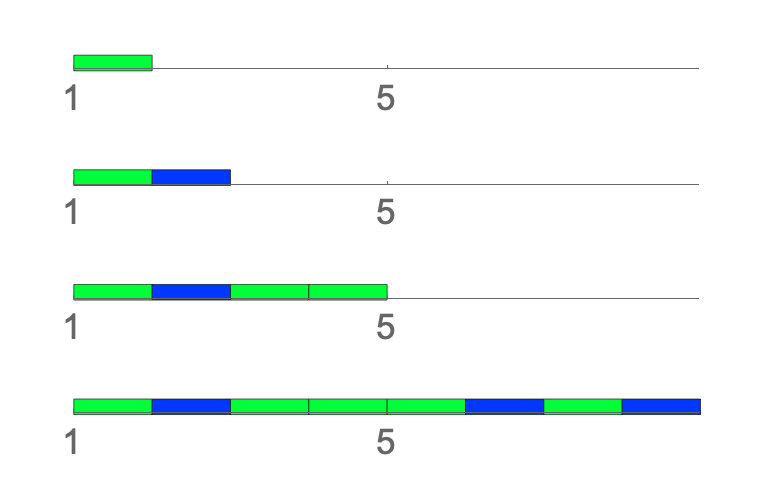
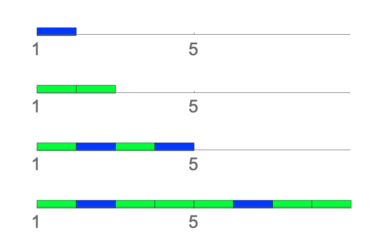
Figure 3. The $\displaystyle A$ tile (top left) and the $\displaystyle B$ tile (top right) with 1-, 2, and 3-supertiles below

The transition matrix is $\displaystyle M=\left(\begin{smallmatrix}1&2\\ 1&0\end{smallmatrix}\right)$ with right Perron eigenvector $\displaystyle(2/3,1/3)$. The system $\displaystyle(\mathcal{S}_{PD},\operatorname{\sigma})$ has a unique shift-invariant probability measure $\displaystyle\mu$ for which $\displaystyle\mu([A])=2/3$, $\displaystyle\mu([B])=1/3$, and all other measures can be deduced from the fact that $\displaystyle\mu(\mathcal{S}_{PD}^{n}([C]))=2^{-n}\mu([C])$. $\displaystyle\Diamond$

2.3. Addresses and $\displaystyle n$-cylinders

A substitution is said to be recognizable if there is some $\displaystyle R>0$ such that if $\displaystyle\boldsymbol{\tau},\boldsymbol{\tau}^{\prime}\in{\Sigma}$ and $\displaystyle\boldsymbol{\tau}[n-R,..n+R]=\boldsymbol{\tau}^{\prime}[n-R,..n+R]$, then $\displaystyle\boldsymbol{\tau}(n)$ and $\displaystyle\boldsymbol{\tau}^{\prime}(n)$ are in exactly the same supertile and location within it. A substitution that is recognizable can be broken down into supertiles and ‘desubstituted’ in a certain sense, if we think of the substitution as acting on $\displaystyle{\Sigma}$.

For $\displaystyle\boldsymbol{\tau}=\{\alpha_{n}\}_{n\in\mathbb{Z}}$, we certainly can define $\displaystyle\mathcal{S}(\boldsymbol{\tau})$ to be $\displaystyle...\mathcal{S}(\alpha_{-1})\mathcal{S}(\alpha_{0})\mathcal{S}(\alpha_{1})...$, but there is not a natural location for the start of $\displaystyle\mathcal{S}(\alpha_{1})$ (or any other supertile). For simplicity we define it so that $\displaystyle\mathcal{S}(\alpha_{1})$ starts at $\displaystyle 1$. Recognizability extends to supertiles of any level, and $\displaystyle\mathcal{S}^{n}(\boldsymbol{\tau})$ is defined so that the $\displaystyle n$-supertile $\displaystyle\mathcal{S}^{n}(\alpha_{1})$ begins at $\displaystyle 1$.

Let the letter $\displaystyle\alpha$ be located at $\displaystyle 1\in\mathbb{Z}$ so that $\displaystyle[\alpha]=\{\boldsymbol{\tau}\in{\Sigma}\text{ with }\boldsymbol{\tau}(1)=\alpha\}.$ We define $\displaystyle\mathcal{S}^{n}([\alpha])=\{\mathcal{S}^{n}(\boldsymbol{\tau}),\boldsymbol{\tau}\in[\alpha]\}$. We know that the topology of $\displaystyle{\Sigma}$ is generated by such sets, shifted so that have 0 sits in all possible locations (see e.g. [14]). For each $\displaystyle n=0,1,2,...$,

(3) $$\mathcal{B}_{n}=\left\{\operatorname{\sigma}^{k}(\mathcal{S}^{n}([\alpha])),\alpha\in{\mathcal{A}}\text{ and }1\leq k\leq|\mathcal{S}^{n}(\alpha)|\right\}$$

forms a partition of $\displaystyle{\Sigma}$. The refining sequence of partitions $\displaystyle\{\mathcal{B}_{n}\}_{n=0}^{\infty}$ is called the canonical partition sequence of $\displaystyle{\Sigma}$. Sets of the form $\displaystyle\operatorname{\sigma}^{k}(\mathcal{S}^{n}([\alpha]))$ with $\displaystyle 1\leq k\leq|\mathcal{S}^{n}(\alpha)|$ are called $\displaystyle n$-cylinders.

Remark 2.4.

There may be a difference between $\displaystyle[\mathcal{S}(\alpha)]$ and $\displaystyle\mathcal{S}([\alpha])$, if there are allowable words that are the same word as $\displaystyle\mathcal{S}(\alpha)$ but that are not actually supertiles by recognition. Our use of the term ‘cylinder’ in ‘$\displaystyle n$-cylinder’ may thus be nonstandard.

The domain of $\displaystyle\mathcal{S}$ is the alphabet of addresses. It is the subset of $\displaystyle{\mathcal{A}}\times\mathbb{N}$ given by

(4) $$\mathsf{A}=\{{\mathsf{a}}:=(\alpha,j)\text{ such that }1\leq j\leq|\mathcal{S}(\alpha)|\}.$$

The projection maps $\displaystyle\pi_{\mathcal{A}}({\mathsf{a}})$ and $\displaystyle\pi_{\mathbb{N}}({\mathsf{a}})$ are used when needed. Elements of $\displaystyle\mathsf{A}$ are used in two crucial ways. One is to specify the word $\displaystyle\mathcal{S}({\mathsf{a}}):=\operatorname{\sigma}^{j}(\mathcal{S}(\alpha))$. The other is to identify the the letter in the $\displaystyle j$th position of $\displaystyle\mathcal{S}(\alpha)$, which is the letter at $\displaystyle 0$ in $\displaystyle\operatorname{\sigma}^{j}(\mathcal{S}(\alpha))$ and so is denoted $\displaystyle\mathcal{S}({\mathsf{a}})_{0}$.

The position of the supertile at the origin in any $\displaystyle\boldsymbol{\tau}\in{\Sigma}$ is indexed by the domain $\displaystyle\mathsf{A}$ and is, by recognizability, unique. When $\displaystyle\boldsymbol{\tau}(0)$ is in the $\displaystyle j$th spot of the $\displaystyle 1$-supertile $\displaystyle\mathcal{S}(\alpha)$, we identify its $\displaystyle 1$-address as $\displaystyle{\boldsymbol{{\mathsf{a}}}}_{{1}}(\boldsymbol{\tau})=(\alpha,j)={\mathsf{a}}\in\mathsf{A}$. Equivalently, $\displaystyle\boldsymbol{\tau}\in\operatorname{\sigma}^{j}(\mathcal{S}[\alpha])$. The $\displaystyle 1$-cylinder of $\displaystyle{\mathsf{a}}=(\alpha,j)$ is defined to be

$$[\mathcal{S}({\mathsf{a}})]=\{\boldsymbol{\tau}\in{\Sigma}\text{ such that }{\boldsymbol{{\mathsf{a}}}}_{{1}}(\boldsymbol{\tau})={\mathsf{a}}\}=\operatorname{\sigma}^{j}(\mathcal{S}([\alpha])).$$

The position of $\displaystyle\boldsymbol{\tau}(0)$’s 1-supertile inside of its 2-supertile is uniquely determined and can be labeled by $\displaystyle\mathsf{A}$. Thus for any $\displaystyle\boldsymbol{\tau}\in{\Sigma}$ we can define the 2-address $\displaystyle{\boldsymbol{{\mathsf{a}}}}_{{2}}(\boldsymbol{\tau})=({\mathsf{a_{1}}},{\mathsf{a_{2}}})$ if $\displaystyle\boldsymbol{\tau}(0)$ is in a 1-supertile of type $\displaystyle\pi_{\mathcal{A}}({\mathsf{a_{1}}})=\alpha_{1}$ in position $\displaystyle\pi_{\mathbb{N}}({\mathsf{a}}_{1})=j_{1}$, and that supertile is contained in a $\displaystyle 2$-supertile of type $\displaystyle\pi_{\mathcal{A}}({\mathsf{a}}_{2})=\alpha_{2}$ at position $\displaystyle\pi_{\mathbb{N}}({\mathsf{a}}_{2})=j_{2}$. There is an appropriate $\displaystyle k\in\{1,2,...,|\mathcal{S}^{2}(\alpha_{2})|\}$ for which $\displaystyle\mathcal{S}({\mathsf{a}}_{1},{\mathsf{a}}_{2})=\operatorname{\sigma}^{k}(\mathcal{S}^{2}(\alpha_{2}))$.

Recognizability implies that for all $\displaystyle n\in\mathbb{N}$ the position of $\displaystyle\boldsymbol{\tau}(0)$’s $\displaystyle(n-1)$-supertile inside its $\displaystyle n$-supertile can be uniquely determined and can be labelled by $\displaystyle\mathsf{A}$. Every $\displaystyle\boldsymbol{\tau}\in{\Sigma}$ contains a nested sequence of $\displaystyle n$-supertiles containing the origin that tells us which partition elements it belongs inside.

Consider the 0-cylinder of type $\displaystyle\alpha$, defined in the 0-level canonical partition (3) to be $\displaystyle\operatorname{\sigma}([\alpha])=\{\boldsymbol{\tau}\in{\Sigma}\,|\,\boldsymbol{\tau}(0)=\alpha\}$. Since $\displaystyle\boldsymbol{\tau}(0)$ is determined by $\displaystyle{\boldsymbol{{\mathsf{a}}}}_{{1}}(\boldsymbol{\tau})$, the 0-cylinder of type $\displaystyle\alpha$ is the union of 1-cylinders that have $\displaystyle\alpha$ at the origin. This gives us a transition rule for addresses as a Markov chain. The set of all positions $\displaystyle\alpha$ appears in 1-supertiles is

(5) $${\mathsf{T}({\alpha})}=\{{\mathsf{b}}\in\mathsf{A}\,|\,\mathcal{S}({\mathsf{b}})_{0}=\alpha\}=\{(\beta,j)\in\mathsf{A}\,|\,\alpha\text{ is the }j\text{th letter of }\mathcal{S}(\beta)\}.$$

If $\displaystyle\pi_{\mathcal{A}}({\mathsf{a}})=\alpha$ we write $\displaystyle{\mathsf{T}({{\mathsf{a}}})}={\mathsf{T}({\alpha})}$. For each $\displaystyle\alpha\in{\mathcal{A}}$ we have $\displaystyle\operatorname{\sigma}([\alpha])=\bigcup_{{\mathsf{b}}\in{\mathsf{T}({\alpha})}}[\mathcal{S}({\mathsf{b}})].$

Definition 2.5.

We say $\displaystyle{\boldsymbol{{\mathsf{a}}}}=({\mathsf{a}}_{1},{\mathsf{a}}_{2},...)\in\mathsf{A}^{\mathbb{N}}\cup\mathsf{A}^{\infty}$ is an address if $\displaystyle{\mathsf{a}}_{k}\in{\mathsf{T}({\alpha_{k-1}})}$ for all $\displaystyle 1\leq k\leq|{{\boldsymbol{{\mathsf{a}}}}}|$. The set of all addresses of lengths $\displaystyle n$, $\displaystyle\infty$, or “any” are denoted $\displaystyle\mathbf{A}_{n},\mathbf{A}_{\infty},$ and $\displaystyle\mathbf{A}$, respectively. For $\displaystyle\boldsymbol{\tau}\in{\Sigma}$, the $\displaystyle n$-address of $\displaystyle\boldsymbol{\tau}$, denoted $\displaystyle{\boldsymbol{{\mathsf{a}}}}_{{n}}(\boldsymbol{\tau})$, is the address of $\displaystyle\boldsymbol{\tau}(0)$’s $\displaystyle n$-supertile.

When $\displaystyle n<\infty$ and $\displaystyle{\boldsymbol{{\mathsf{a}}}}=({\mathsf{a}}_{1}{\mathsf{a}}_{2},...,{\mathsf{a}}_{n})$, we define the $\displaystyle n$-supertile addressed by $\displaystyle{\boldsymbol{{\mathsf{a}}}}$ to be $\displaystyle\mathcal{S}({\boldsymbol{{\mathsf{a}}}})=\operatorname{\sigma}^{j}(\mathcal{S}^{n}(\pi_{\mathcal{A}}({\mathsf{a}}))),$ for the appropriate value of $\displaystyle j$. Similarly the address corresponds to the $\displaystyle n$-cylinder denoted $\displaystyle[\mathcal{S}({\boldsymbol{{\mathsf{a}}}})]=\operatorname{\sigma}^{j}(\mathcal{S}^{n}([\pi_{\mathcal{A}}({\mathsf{a}})]))$. The length of $\displaystyle{\boldsymbol{{\mathsf{a}}}}$ is the level of the supertile $\displaystyle{\boldsymbol{{\mathsf{a}}}}$ represents. If $\displaystyle|{\boldsymbol{{\mathsf{a}}}}|=n<\infty$, the type of $\displaystyle{\boldsymbol{{\mathsf{a}}}}$ is $\displaystyle\alpha_{n}$ and $\displaystyle{\boldsymbol{{\mathsf{a}}}}$ specifies an exact location (or domain) for $\displaystyle\mathcal{S}^{n}(\alpha_{n})$.

An address can be thought of as instructions: First, place a supertile of type $\displaystyle\alpha_{1}$ so that the origin is in the $\displaystyle j_{1}$th spot. Then, slide a copy of $\displaystyle\mathcal{S}^{2}(\alpha_{2})$ to match its $\displaystyle j_{2}$’th 1-supertile to the one in place already. Then move a copy of $\displaystyle\mathcal{S}^{3}(\alpha_{3})$ to match its $\displaystyle j_{3}$th 2-supertile to the existing one, and so on. Figure 4 illustrates the process for the 3-supertile $\displaystyle\mathcal{S}_{PD}(B2,A2,A1)$.

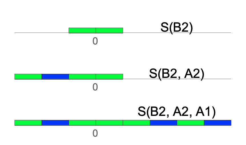
Figure 4. Building a supertile from an address string

Any two addresses $\displaystyle{\boldsymbol{{\mathsf{a}}}}$ and $\displaystyle{\boldsymbol{{\mathsf{a}}}}^{\prime}$ that share a common prefix $\displaystyle{\boldsymbol{{\mathsf{a}}}}_{{n}}$ correspond to elements of $\displaystyle{\Sigma}$ that have the same $\displaystyle n$-supertile in the same location at the origin. Thus both $\displaystyle[\mathcal{S}({\boldsymbol{{\mathsf{a}}}})]$ and $\displaystyle[\mathcal{S}({\boldsymbol{{\mathsf{a}}}}^{\prime})]$ are contained in $\displaystyle[\mathcal{S}({\boldsymbol{{\mathsf{a}}}}_{{n}})]$. Each $\displaystyle{\boldsymbol{{\mathsf{a}}}}\in\mathbf{A}_{n-1}$ addresses an $\displaystyle(n-1)$-supertile of some type $\displaystyle\alpha_{n-1}$ and therefore can be contained in any $\displaystyle n$-supertile from $\displaystyle{\mathsf{T}({\alpha_{n-1}})}$. That means

$$[\mathcal{S}({\boldsymbol{{\mathsf{a}}}})]=\bigcup_{{\mathsf{b}}\in{\mathsf{T}({\alpha_{n-1}})}}[\mathcal{S}({\boldsymbol{{\mathsf{a}}}},{\mathsf{b}})].$$

Every element of $\displaystyle\mathcal{B}_{n}$ arises in this way, showing that $\displaystyle\mathcal{B}_{n}$ is a refinement of $\displaystyle\mathcal{B}_{n-1}$ for all $\displaystyle n\in\mathbb{N}$. Since the measures of all partition elements go to zero, the sequence refines to points almost everywhere. Addresses may fail to uniquely specify an element of $\displaystyle{\Sigma}$, but we will see this is a measure-0 event. Note that extending an address corresponds to identifying a higher-order supertile around 0.

3. The functions $\displaystyle\Phi$ and $\displaystyle\mathfrak{F}$

In this section we define the maps that make up the measurable conjugacy $\displaystyle\Phi:({\Sigma},\operatorname{\sigma},\mu)\to([0,1],\mathfrak{F},m)$, illustrating the process with the period-doubling substitution. Proofs will follow in the next section. Readers may well be reminded of many constructions using similar ideas, for instance [3, 12], Anosov flows, Veech rectangles, and a variety of tower-related constructions.

The next two figures encapsulate the ideas behind the construction of $\displaystyle\Phi$, the flow view, and $\displaystyle\mathfrak{F}$. Figure 5 illustrates how the dual subdivision graph helps locate supertiles vertically using the $\displaystyle 3$-supertile from figure 4. This figure is behind the definition of $\displaystyle\Phi$ .

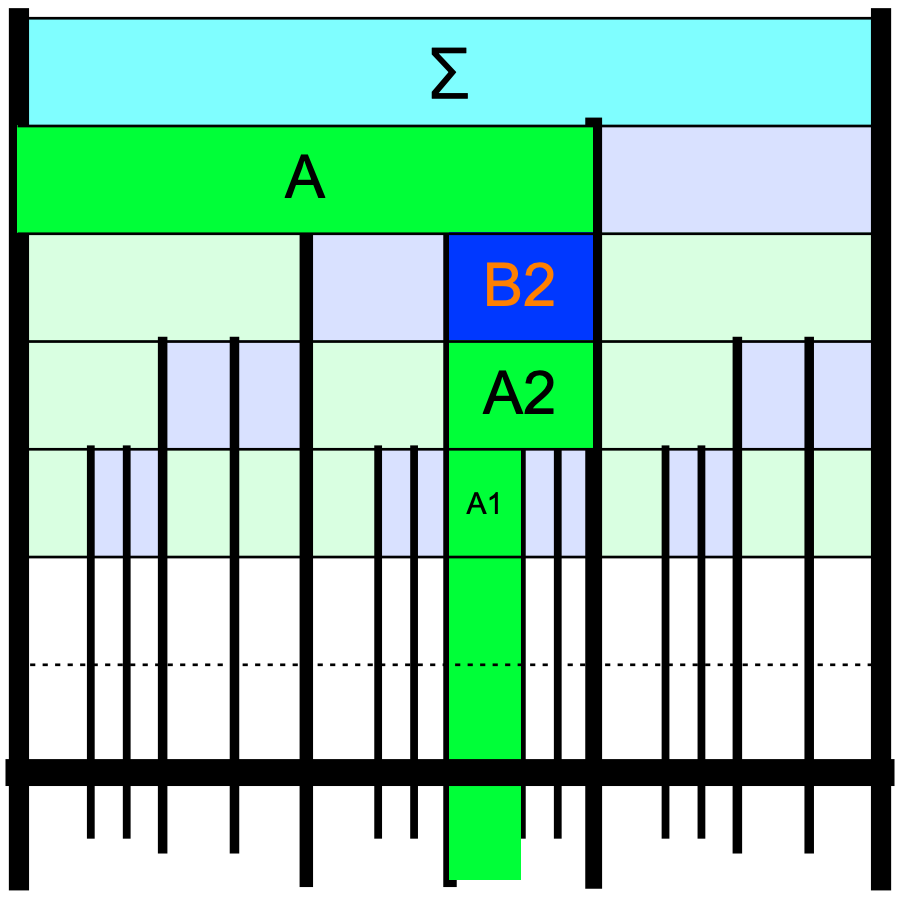
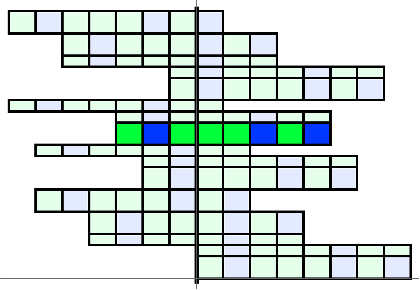
Figure 5. The highlighted path in the dual subdivision leads to the correct interval to place $\displaystyle\mathcal{S}_{PD}(B2,A2,A1)$ within the level-3 flow view

Figure 6 illustrates how shifting a supertile leads to a change in address, again using the supertile from figure 4. The author does not know an obvious way to see the shift in the subdivision graph directly, but the upcoming definition of $\displaystyle\mathfrak{F}$ (equation (11)) captures it in a formula. Importantly, these figures show how the interval exchange transformation arises.

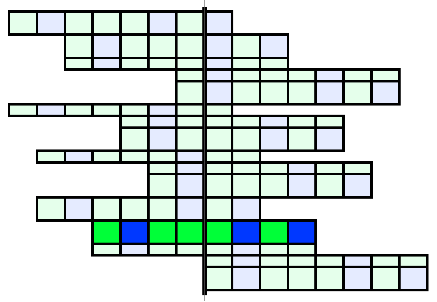
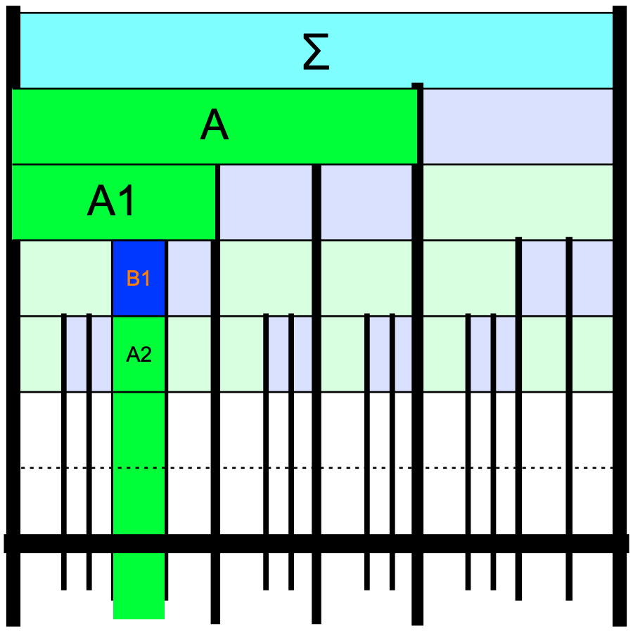
Figure 6. The shifted supertile $\displaystyle\operatorname{\sigma}(\mathcal{S}_{PD}(B2,A2,A1))$ has address $\displaystyle(A1,B1,A2)$

The standard set of assumptions to be used are as follows. The substitution $\displaystyle\mathcal{S}$ should be recognizable and its subshift should be minimal in the sense that every orbit is dense. The measure $\displaystyle\mu$ is assumed to be a shift-invariant Borel probability measure. With these assumptions, letters with zero frequency and other technical difficulties are avoided.

3.1. Definition of $\displaystyle\Phi$

In this section we construct a partition sequence of $\displaystyle[0,1)$ to match up with the canonical partition sequence of $\displaystyle{\Sigma}$. A partition element $\displaystyle{\mathbf{I}}({\boldsymbol{{\mathsf{a}}}}_{{n}})$ in $\displaystyle[0,1)$ of length $\displaystyle\mu([\mathcal{S}({\boldsymbol{{\mathsf{a}}}}_{{n}})])$ is assigned to each $\displaystyle n$-cylinder in a way that preserves inclusion. The partition sequence in $\displaystyle{\Sigma}$ refines to points so the map $\displaystyle\Phi$ can be thought of intuitively as infinite intersections, but we define it as a nondecreasing limit of left endpoints given by partial sums $\displaystyle\Phi_{n}:\mathcal{B}_{n}\to[0,1)$. The $\displaystyle n$-th level flow view displays $\displaystyle\mathcal{S}({\boldsymbol{{\mathsf{a}}}}_{{n}})$ at a height $\displaystyle\Phi_{n}({\boldsymbol{{\mathsf{a}}}}_{{n}})$ with vertical thickness $\displaystyle\mu([\mathcal{S}({\boldsymbol{{\mathsf{a}}}}_{{n}})])$.

To start, we need to choose an initial partition of $\displaystyle[0,1)$. Since $\displaystyle\mu$ is a probability measure we know $\displaystyle\sum_{\alpha\in{\mathcal{A}}}\mu([\alpha])=1$, so for each $\displaystyle\alpha\in{\mathcal{A}}$, choose a left endpoint $\displaystyle{\Phi}_{0}(\alpha)\in[0,1)$ such that the intervals $\displaystyle{\mathbf{I}}(\alpha):=[{\Phi}_{0}(\alpha),{\Phi}_{0}(\alpha)+\mu([\alpha]))$ cover $\displaystyle[0,1)$. The initial partition is $\displaystyle\mathcal{I}_{0}=\{{\mathbf{I}}(\alpha),\alpha\in{\mathcal{A}}\}$.

The left side of figure 7 shows the initial partitions at the top of the subdivision graph using the choice $\displaystyle{\Phi}_{0}(A)=0,\,{\Phi}_{0}(B)=2/3$ . Any element $\displaystyle\boldsymbol{\tau}\in{\Sigma}$ with $\displaystyle\boldsymbol{\tau}(0)=A$ will ultimately be sent somewhere in the interval $\displaystyle[0,2/3]$. Likewise if $\displaystyle\boldsymbol{\tau}(0)=B$ then $\displaystyle\Phi(\boldsymbol{\tau})\in[2/3,1]$.

Figure 7. The initial partition for $\displaystyle\mathcal{S}_{PD}$: dual subdivision graph (left), level-0 flow view (right)

Recall that for $\displaystyle{\mathsf{b}}=(\beta,j)\in\mathsf{A}{}$, $\displaystyle\mu([\mathcal{S}({\mathsf{b}})])=\mu(\mathcal{S}([\beta]))=\mu([\beta])/\lambda.$ We have

(6) $$\mu([\alpha])=\sum_{{\mathsf{b}}\in{\mathsf{T}({\alpha})}}\mu([\mathcal{S}(\beta)])=\sum_{{\mathsf{b}}\in{\mathsf{T}({\alpha})}}\mu([\beta])/\lambda.$$

That means for each $\displaystyle\alpha\in{\mathcal{A}}$ we can partition $\displaystyle[0,\mu([\alpha]))$ into intervals of these lengths. Let the ‘left endpoint’ function $\displaystyle{\phi}:{\mathsf{T}({\alpha})}\to[0,\mu([\alpha]))$ record the left endpoints of this partition and define $\displaystyle{\phi}({\mathsf{a}})={\phi}(\alpha)$ for $\displaystyle\alpha=\pi_{\mathcal{A}}({\mathsf{a}})$. We have

(7) $$\left[0,\mu([\alpha])\right)=\bigcup_{{\mathsf{b}}\in{\mathsf{T}({{\mathsf{a}}})}}\left[{\phi}({\mathsf{b}}),\,{\phi}({\mathsf{b}})+\frac{\mu([\pi_{\mathcal{A}}({\mathsf{b}})])}{\lambda}\right).$$

Figure 8 shows the choice of $\displaystyle{\phi}$ to be used for the period-doubling flow view.

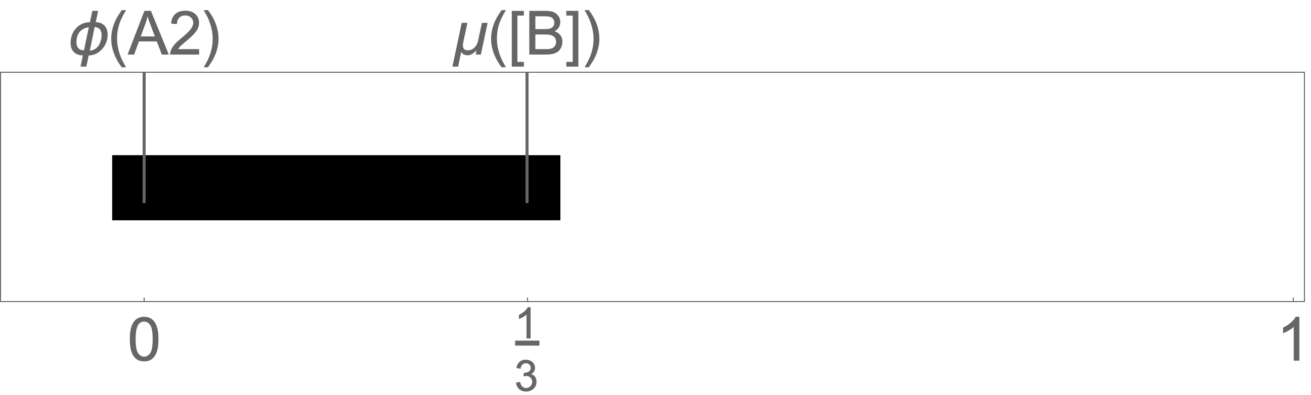
Figure 8. Our choice of initial partition for $\displaystyle\mathcal{S}_{PD}$

The orders of the subintervals chosen for $\displaystyle{\phi}$ are conveniently expressed as a fixed dual substitution $\displaystyle{\mathcal{S}_{*}}$. The row corresponding to $\displaystyle\alpha$ in the substitution matrix of $\displaystyle M$ is the column for $\displaystyle\alpha$ in the matrix of $\displaystyle{\mathcal{S}_{*}}$, so $\displaystyle{\mathcal{S}_{*}}(\alpha)$ contains the composition of letters seen in $\displaystyle{\mathsf{T}({\alpha})}$. To move the partition of $\displaystyle[0,\mu([\alpha]))$ into the correct location in $\displaystyle[0,1)$ we add $\displaystyle{\Phi}_{0}([\alpha])$. Let $\displaystyle{\mathsf{b}}\in\mathsf{A}$ with $\displaystyle{\mathsf{b}}\in T_{\alpha}$. Then

$${\Phi}_{1}({\mathsf{b}})={\Phi}_{0}(\alpha)+{\phi}({\mathsf{b}})\,\text{ and }\,{\mathbf{I}}({\mathsf{b}})=\left[{\Phi}_{1}({\mathsf{b}}),{\Phi}_{1}({\mathsf{b}})+\mu([\mathcal{S}({\mathsf{b}})])\right)$$

So $\displaystyle\mathcal{I}_{1}=\left\{{\mathbf{I}}({\mathsf{a}}),\,{\mathsf{a}}\in\mathsf{A}\right\}$ refines partition $\displaystyle\mathcal{I}_{0}$ and $\displaystyle m({\mathbf{I}}({\mathsf{a}}))=\mu([\mathcal{S}({\mathsf{a}})])$ for all $\displaystyle{\mathsf{a}}\in\mathsf{A}$.

The first refinements of the period doubling flow view appear in figure 9. Since $\displaystyle{\mathsf{T}({A})}=\{A1,B1,B2\}$ and $\displaystyle{\mathsf{T}({B})}=\{A2\},$ we choose the dual substitution $\displaystyle{\mathcal{S}_{*}}:A\to ABB$ and $\displaystyle B\to A.$ For $\displaystyle{\phi}$ and $\displaystyle{\Phi}_{1}$ that gives:

$${\Phi}_{1}(A1)=0+0,\quad{\Phi}_{1}(B1)=0+1/3,\quad{\Phi}_{1}(B2)=0+1/2,\text{ and }{\Phi}_{1}(A2)=2/3+0.$$

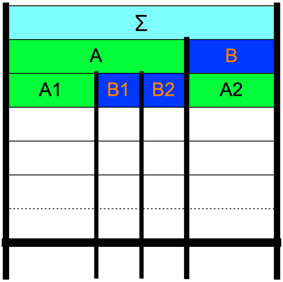
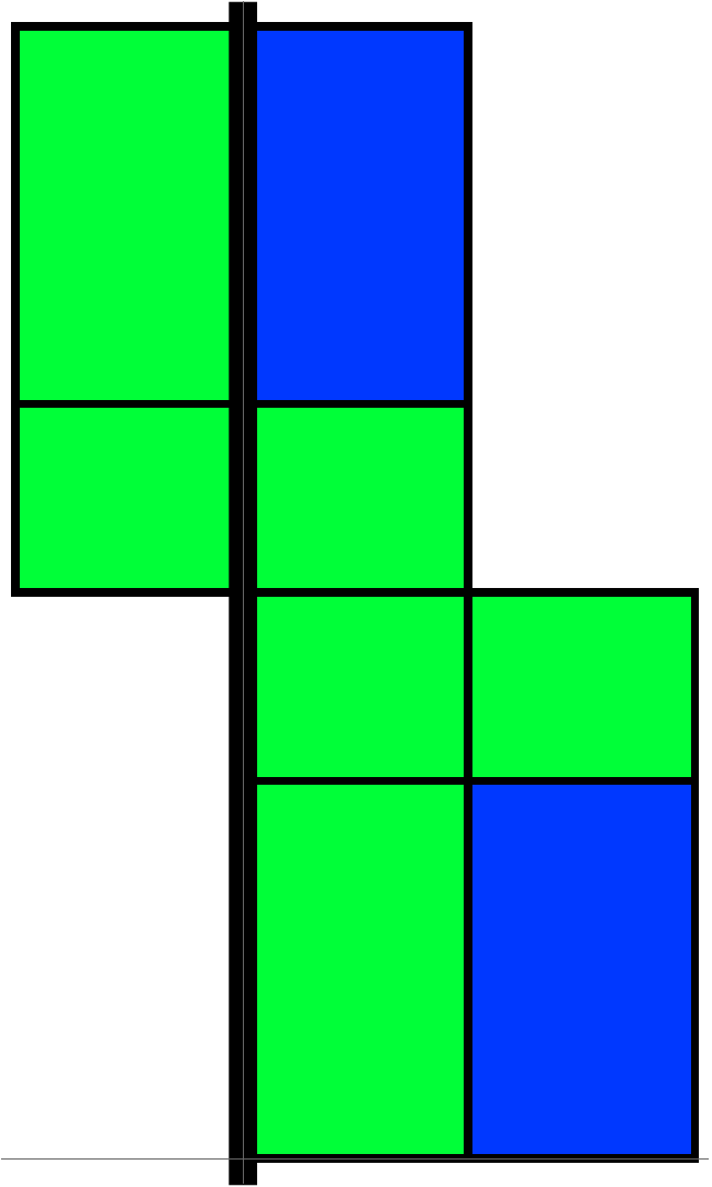
Figure 9. The first dual subdivision and the level-1 flow view for $\displaystyle\mathcal{S}_{PD}$

To build the flow view, place a copy of each of the supertiles in their positions horizontally, then raise them to the height and thickness given by the interval of the same address. This represents the $\displaystyle n$-cylinder set of all tiling that have that supertile at the origin in that position, and its Lebesgue measure matches its $\displaystyle\mu$-measure.

This process is used to refine intervals at level $\displaystyle(n-1)$ to level $\displaystyle n$ in general, but the reader may benefit from seeing one more level. The refinement $\displaystyle\mathcal{I}_{2}$ is given by sets of the form $\displaystyle{\mathbf{I}}({\mathsf{a}}_{1},{\mathsf{a}}_{2})$, where $\displaystyle({\mathsf{a}}_{1},{\mathsf{a}}_{2})\in\mathbf{A}_{2}$. We construct our refinement so that each $\displaystyle{\mathbf{I}}({\mathsf{a}}_{1})\in\mathcal{I}_{1}$ is partitioned by $\displaystyle\{{\mathbf{I}}({\mathsf{a_{1}}},{\mathsf{a_{2}}}),{\mathsf{a}}_{2}\in{\mathsf{T}({{\mathsf{a}}_{1}})}\}$ placed in the order given by $\displaystyle{\mathcal{S}_{*}}$.

Suppose $\displaystyle\pi_{\mathcal{A}}({\mathsf{a}}_{i})=\alpha_{i}$ for $\displaystyle i=1,2$. Because $\displaystyle\mu$ is invariant, and because the 2-cylinder set $\displaystyle[\mathcal{S}({\mathsf{a}}_{1},{\mathsf{a}}_{2})]$ is a shift of the 2-cylinder $\displaystyle\mathcal{S}^{2}([\alpha_{2}])$ we have

$$\mu([\mathcal{S}({\mathsf{a}}_{1})])=\sum_{{\mathsf{a}}_{2}\in{\mathsf{T}({{\mathsf{a}}_{1}})}}\mu([\mathcal{S}({\mathsf{a}}_{1},{\mathsf{a}}_{2})])=\sum_{{\mathsf{a}}_{2}\in{\mathsf{T}({{\mathsf{a}}_{1}})}}\mu([\pi_{\mathcal{A}}({\mathsf{a}}_{2})])/\lambda^{2}.$$

Because the interval $\displaystyle[0,\mu([\mathcal{S}(\alpha_{1})]))$ is scaled by $\displaystyle 1/\lambda$ from $\displaystyle[0,\mu([\alpha_{1}]))$, we use $\displaystyle{\phi}({\mathsf{a}}_{2})/\lambda$ to partition it. This preserves the order given by $\displaystyle{\mathcal{S}_{*}}$. A scaled-down copy of the partition of $\displaystyle\alpha_{1}$ is placed on every $\displaystyle{\mathbf{I}}({\mathsf{a}}_{1})$ where $\displaystyle\pi_{\mathcal{A}}({\mathsf{a}}_{1})=\alpha_{1}$. That is, take $\displaystyle{\Phi}_{1}(\mathcal{S}({\mathsf{a}}_{1}))$ and add on $\displaystyle{\phi}({\mathsf{a}}_{2})/\lambda$:

$${\Phi}_{2}({\mathsf{a}}_{1},{\mathsf{a}}_{2})={\Phi}_{1}({\mathsf{a}}_{1})+{\phi}({\mathsf{a}}_{2})/\lambda\quad$$

We define $\displaystyle{\mathbf{I}}({\mathsf{a}}_{1},{\mathsf{a}}_{2})=[{\Phi}_{2}({\mathsf{a}}_{1},{\mathsf{a}}_{2}),{\Phi}_{2}({\mathsf{a}}_{1},{\mathsf{a}}_{2})+\mu([\pi_{\mathcal{A}}({\mathsf{a}}_{2})])/\lambda^{2})$. See figure 10.

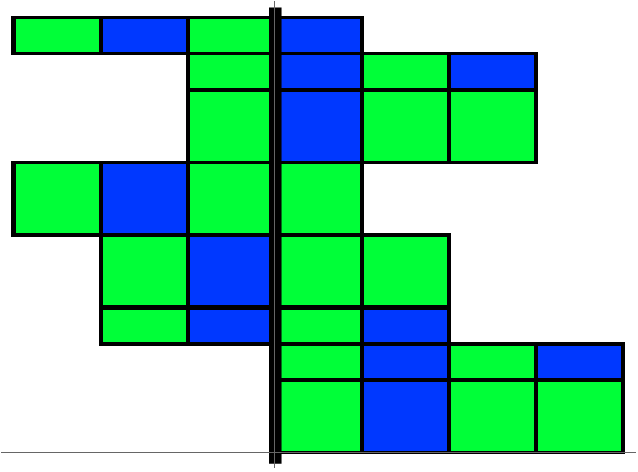
Figure 10. The level-2 dual subdivision and flow view for $\displaystyle\mathcal{S}_{PD}$

From here the refinements follow the same pattern and we can define the function $\displaystyle{\Phi}_{n}:\mathbf{A}_{n}\to[0,1)$ recursively or directly. For notational convenience consider $\displaystyle\mathbf{A}_{0}=\mathsf{A}$ and let $\displaystyle\Phi_{0}:\mathsf{A}\to[0,1]$ be $\displaystyle\Phi_{0}({\mathsf{a}}):=\Phi_{0}(\pi_{\mathcal{A}}({\mathsf{a}}))$. If $\displaystyle{\boldsymbol{{\mathsf{a}}}}=({\mathsf{a}}_{1},{\mathsf{a}}_{2},...{\mathsf{a}}_{n})$, then

(8) $${\Phi}_{n}({\boldsymbol{{\mathsf{a}}}})={\Phi}_{n-1}({\mathsf{a}}_{1}\,...,{\mathsf{a}}_{n-1})+{\phi}({\mathsf{a}}_{n})/\lambda^{n-1}={\Phi}_{0}({\mathsf{a}}_{1})\ +\sum_{k=1}^{n}{\phi}({\mathsf{a}}_{k})/\lambda^{k-1}.$$

The interval corresponding to $\displaystyle{\boldsymbol{{\mathsf{a}}}}$ is thus

$${\mathbf{I}}({\boldsymbol{{\mathsf{a}}}})=[{\Phi}_{n}({\boldsymbol{{\mathsf{a}}}}),{\Phi}_{n}({\boldsymbol{{\mathsf{a}}}})+\mu(\pi_{\mathcal{A}}({\mathsf{a}}_{n})))/\lambda^{n})=[{\Phi}_{n}({\boldsymbol{{\mathsf{a}}}}),{\Phi}_{n}({\boldsymbol{{\mathsf{a}}}})+\mu([\mathcal{S}({\boldsymbol{{\mathsf{a}}}})])),$$

making the Lebesgue measure of $\displaystyle{\mathbf{I}}({\boldsymbol{{\mathsf{a}}}})$ is equal to $\displaystyle\mu([\mathcal{S}({\boldsymbol{{\mathsf{a}}}})])$. We define the canonical partition sequence of $\displaystyle[0,1)$ given by $\displaystyle{\mathcal{S}_{*}}$ to be $\displaystyle\mathcal{I}_{n}=\{{\mathbf{I}}({\mathsf{a_{1}}},{\mathsf{a_{2}}},...{\mathsf{a_{n}}})\text{ such that }({\mathsf{a_{1}}},{\mathsf{a_{2}}},...{\mathsf{a_{n}}})\in\mathbf{A}_{n}\}.$

Definition 3.1.

The coordinate map given by $\displaystyle{\mathcal{S}_{*}}$ is the map $\displaystyle\Phi:{\Sigma}\to[0,1]$ given by

(9) $$\Phi(\boldsymbol{\tau})=\lim_{n\to\infty}\Phi_{n}({\boldsymbol{{\mathsf{a}}}}_{{n}}(\boldsymbol{\tau}))={\Phi}_{0}({\mathsf{a}}_{1})\ +\sum_{k=1}^{\infty}{\phi}({\mathsf{a}}_{k})/\lambda^{k-1},\text{ where }{\boldsymbol{{\mathsf{a}}}}(\boldsymbol{\tau})=({\mathsf{a_{1}}},{\mathsf{a_{2}}},...).$$

The flow view given by $\displaystyle{\mathcal{S}_{*}}$ is the graph of a canonical isomorphism $\displaystyle\Phi$, with each $\displaystyle\boldsymbol{\tau}\in{\Sigma}$ shown at the height $\displaystyle\Phi(\boldsymbol{\tau})$. The $\displaystyle n$th level flow view is the graph of $\displaystyle\Phi_{n}$. The fact that coordinate maps are measure-theoretic isomorphisms is deferred to the next section.

Figure 11 shows the flow view for the substitution $\displaystyle 1\to 1\,3\,2\,,2\to 2\,3\,1\,,3\to 3\,1\,3$. This substitution is constant-length with expansion $\displaystyle\lambda=3$ and has a period-2 substructure.

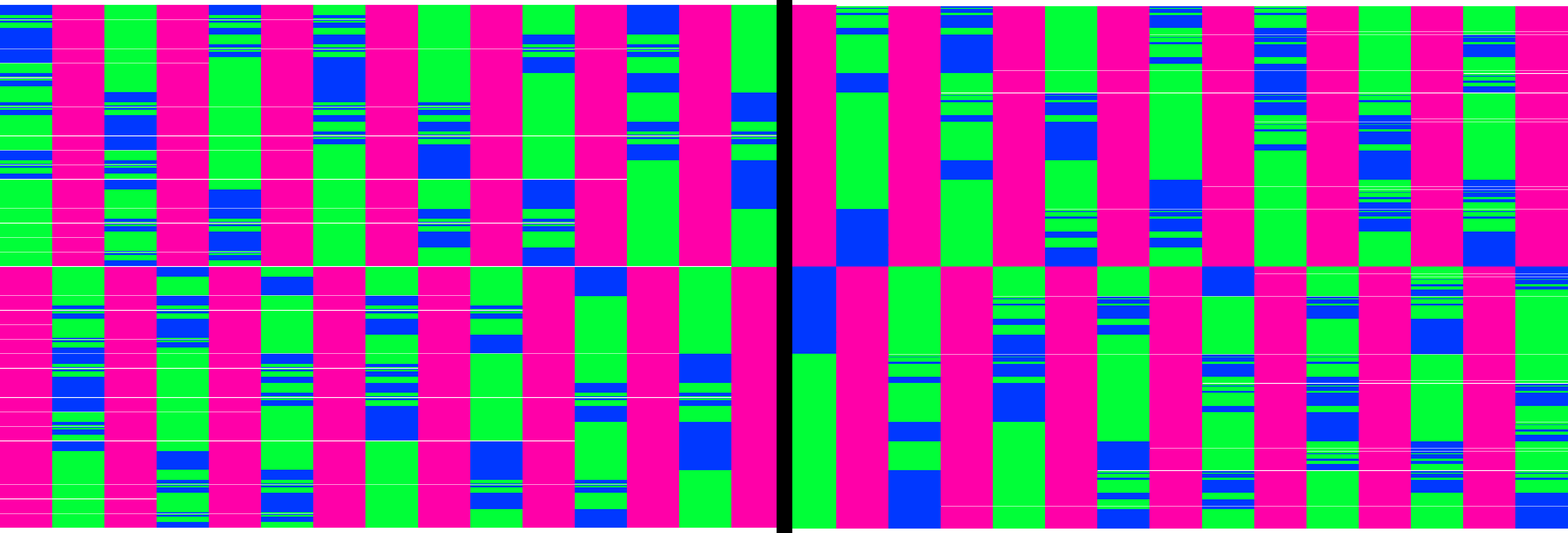
Figure 11. This substitution has nontrivial “height” of 2 [17]

3.2. Definition of $\displaystyle\mathfrak{F}$

Shifts in $\displaystyle{\Sigma}$ cause changes in the addresses in a way that is captured almost everywhere by an especially simple Vershik map on a stationary Bratteli diagram. It is already interesting to consider this system, but we need only the Vershik map, and solely as a bookkeeping device. For the interested, we briefly describe the Bratteli diagram first.

The vertex set at each level of our Bratteli diagram (except the top) is $\displaystyle\mathsf{A}$. The edges into a vertex $\displaystyle{\mathsf{a}}=(\alpha,j)$ at level $\displaystyle n$ are from $\displaystyle\{{\mathsf{b}}=(\beta,k),1\leq k\leq|\mathcal{S}(\beta)|\}$ at level $\displaystyle(n-1)$, where $\displaystyle\beta$ is the letter at position $\displaystyle j$ in $\displaystyle\mathcal{S}({\mathsf{a}})$. This must be the case because the level $\displaystyle n$ address letter specifies the type at $\displaystyle(n-1)$, but not the position. We call the edge set $\displaystyle\mathsf{E}$.

This canonical order relates the minimal and maximal paths in the Bratteli diagram to the the first and last positions in supertiles. Together $\displaystyle(\mathsf{A},\mathsf{E})$ form a stationary Bratteli diagram whose path space is given by $\displaystyle\mathbf{A}_{\infty}$. There are exactly $\displaystyle|{\mathcal{A}}|$ minimal and maximal paths in each $\displaystyle\mathbf{A}_{n}$ that address the first and last positions of the $\displaystyle n$-supertile of each type, and we denote these by $\displaystyle\underline{{\boldsymbol{{\mathsf{a}}}}_{{{n}}}}{(\alpha)}$ and $\displaystyle\overline{{\boldsymbol{{\mathsf{a}}}}_{{{n}}}}{(\alpha)},\alpha\in{\mathcal{A}}$.

For any $\displaystyle{\boldsymbol{{\mathsf{a}}}}=({\mathsf{a}}_{1},{\mathsf{a}}_{2},...)\in\mathbf{A}$ define $\displaystyle\mathbf{n}({\boldsymbol{{\mathsf{a}}}})$ to be the first index at which an element of $\displaystyle{\boldsymbol{{\mathsf{a}}}}$ can be increased, i.e. the smallest $\displaystyle k$ for which $\displaystyle{\boldsymbol{{\mathsf{a}}}}_{{[1,...k]}}\neq\overline{{\boldsymbol{{\mathsf{a}}}}_{{{k}}}}{(\alpha)}$ for any $\displaystyle\alpha$.

Definition 3.2.

The Vershik map $\displaystyle{\mathcal{V}}:\mathbf{A}\to\mathbf{A}$ is defined for any $\displaystyle{\boldsymbol{{\mathsf{a}}}}$ for which $\displaystyle\mathbf{n}({\boldsymbol{{\mathsf{a}}}})=N<\infty$ with $\displaystyle{\boldsymbol{{\mathsf{a}}}}=(\overline{{\boldsymbol{{\mathsf{a}}}}_{{{N-1}}}}{(\alpha)},(\alpha_{N},j_{N}),{\mathsf{a}}_{N+1}...)$ to be

(10) $${\mathcal{V}}({\boldsymbol{{\mathsf{a}}}})=\left(\underline{{\boldsymbol{{\mathsf{a}}}}_{{{N-1}}}}{(\beta)},(\alpha_{N},j_{N}+1),{\mathsf{a}}_{N+1},...\right),\text{ where }\beta\text{ is the }(j_{N}+1)\text{th letter of }\mathcal{S}(\alpha_{N}).$$

A return to figures 5 and 6 may be helpful in understanding how the Vershik map keeps track of an address as its tiling is shifted. There is no change to the address of any $\displaystyle k$-supertile where $\displaystyle k>\mathbf{n}({\boldsymbol{{\mathsf{a}}}})$, since the boundary being crossed over is in its interior. The coding inside the $\displaystyle\mathbf{n}({\boldsymbol{{\mathsf{a}}}})$-supertile is increased by one, resetting all of its subtiles to their first positions. The types of those subtiles depends on $\displaystyle\beta$.

We define $\displaystyle\mathbf{n}(\boldsymbol{\tau})=\mathbf{n}({\boldsymbol{{\mathsf{a}}}}(\boldsymbol{\tau}))$, making $\displaystyle{\boldsymbol{{\mathsf{a}}}}_{{\mathbf{n}(\boldsymbol{\tau})}}(\boldsymbol{\tau})$ the address of the lowest-level supertile containing both $\displaystyle\boldsymbol{\tau}$ and $\displaystyle\operatorname{\sigma}(\boldsymbol{\tau})$. That means $\displaystyle{\boldsymbol{{\mathsf{a}}}}_{{[\mathbf{n}(\boldsymbol{\tau})+1,\infty)}}(\boldsymbol{\tau})={\boldsymbol{{\mathsf{a}}}}_{{[\mathbf{n}(\boldsymbol{\tau})+1,\infty)}}(\operatorname{\sigma}(\boldsymbol{\tau}))$ and we say that $\displaystyle{\boldsymbol{{\mathsf{a}}}}(\boldsymbol{\tau})$ and $\displaystyle{\boldsymbol{{\mathsf{a}}}}(\operatorname{\sigma}(\boldsymbol{\tau}))$ are tail equivalent. The map $\displaystyle{\mathcal{V}}$ was designed to record how the addresses of sequences change under the action of the shift. In lemma 4.6 we will show that for all $\displaystyle\boldsymbol{\tau}\in{\Sigma}$ with $\displaystyle\mathbf{n}({\boldsymbol{{\mathsf{a}}}}(\boldsymbol{\tau}))<\infty$, $\displaystyle{\boldsymbol{{\mathsf{a}}}}(\operatorname{\sigma}(\boldsymbol{\tau}))={\mathcal{V}}({\boldsymbol{{\mathsf{a}}}}(\boldsymbol{\tau})).$

In order to define $\displaystyle\mathfrak{F}$ as a function that commutes with $\displaystyle\operatorname{\sigma}$ we need to give a unique address to almost every $\displaystyle x\in[0,1]$. That requires identifying the partition element that contains $\displaystyle x$ at each level. This is not a problem for the points on which $\displaystyle\Phi$ is invertible, in which case we define $\displaystyle{\boldsymbol{{\mathsf{a}}}}(x)={\boldsymbol{{\mathsf{a}}}}(\Phi^{-1}(x))$.

At points where $\displaystyle\Phi$ is not one-to-one, the proof of proposition 13 shows that $\displaystyle x$ is a partition endpoint. Thus there is a $\displaystyle\boldsymbol{\tau}$ in its preimage for which $\displaystyle x=\Phi(\boldsymbol{\tau})=\Phi_{K}(\boldsymbol{\tau})$ as a finite sum. We choose this preimage and define $\displaystyle{\boldsymbol{{\mathsf{a}}}}(x)={\boldsymbol{{\mathsf{a}}}}(\boldsymbol{\tau})$ and $\displaystyle\mathbf{n}(x)=\mathbf{n}({\boldsymbol{{\mathsf{a}}}}(\boldsymbol{\tau}))$ for this $\displaystyle\boldsymbol{\tau}$. This makes $\displaystyle\mathfrak{F}$ take $\displaystyle x$ along with the elements in the interval above it. For $\displaystyle x\in[0,1]$ with $\displaystyle\mathbf{n}(x)=N<\infty$, define the canonical IIET given by $\displaystyle{\mathcal{S}_{*}}$ to be

(11) $$\mathfrak{F}(x)=x-{\Phi}_{N}({\boldsymbol{{\mathsf{a}}}}_{{N}}(x))+{\Phi}_{N}({\mathcal{V}}({\boldsymbol{{\mathsf{a}}}}_{{N}}(x))).$$

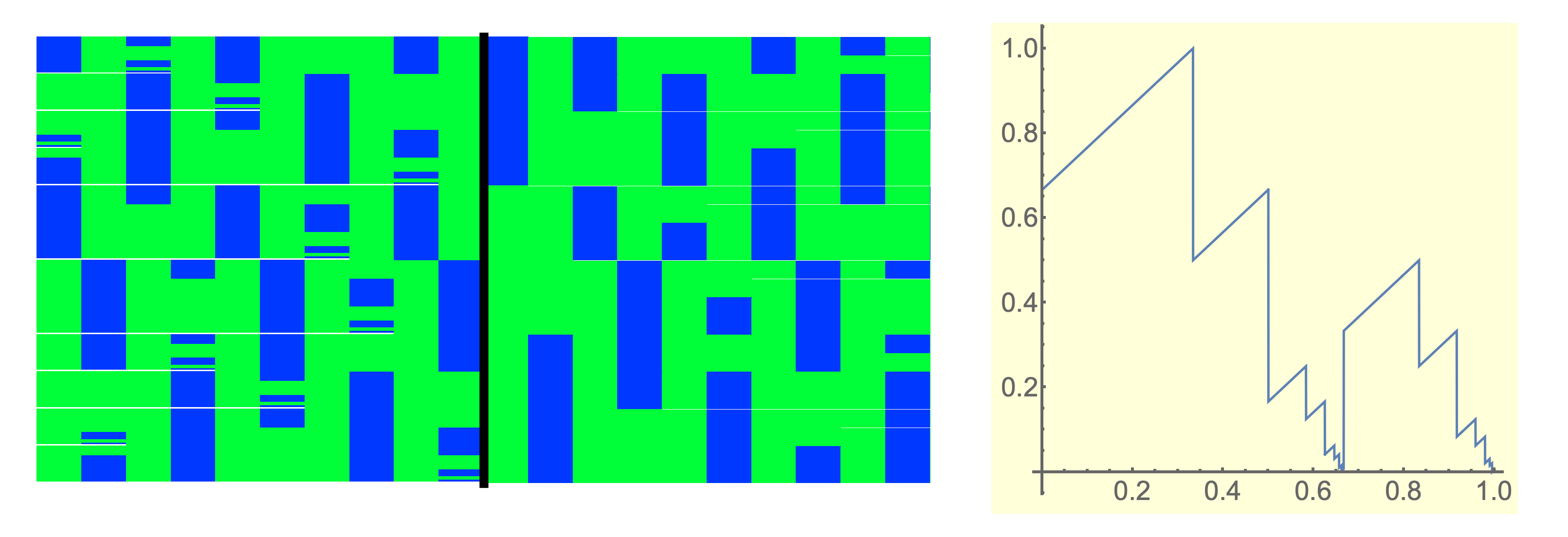
Figure 12. The final results for period-doubling. The blue vertical lines in the IIET connect the ends of jump discontinuities

4. Proofs and properties

Recall our standard assumptions: the substitution $\displaystyle\mathcal{S}$ should be recognizable and its subshift should be minimal in the sense that every orbit is dense. The measure $\displaystyle\mu$ is assumed to be a shift-invariant Borel probability measure. With these assumptions we have the following handy lemma, whose proof we omit.

Lemma 4.1.

If $\displaystyle({\Sigma},\operatorname{\sigma})$ is minimal and $\displaystyle\mu$ is shift invariant, the subset

(12) $${\Sigma}_{0}=\{\boldsymbol{\tau}\in{\Sigma}\,|\,\text{each }{\mathsf{a}}\in\mathsf{A}\text{ appears infinitely often in }{\boldsymbol{{\mathsf{a}}}}(\boldsymbol{\tau})\}$$

has full measure.

4.1. Properties of $\displaystyle\Phi$

The main result is that although $\displaystyle\Phi$ is only a measure-theoretic isomorphism, it is uniformly continuous and 2:1 wherever it is not 1:1.

Proposition 4.2.

Given $\displaystyle\boldsymbol{\tau}\in{\Sigma}$ with $\displaystyle{\boldsymbol{{\mathsf{a}}}}(\boldsymbol{\tau})=\left\{{\mathsf{a}}_{n}\right\}_{n=1}^{\infty}$, the map

(13) $$\Phi(\boldsymbol{\tau})={\Phi}_{0}(\boldsymbol{\tau}(0))+\sum_{n=1}^{\infty}\frac{{\phi}({\mathsf{a}}_{n})}{\lambda^{n-1}}={\Phi}_{K}({{\boldsymbol{{\mathsf{a}}}}}_{K}(\boldsymbol{\tau}))+\sum_{n=K+1}^{\infty}\frac{{\phi}({\mathsf{a}}_{n})}{\lambda^{n-1}}$$

is uniformly continuous everywhere and bijective almost everywhere.

Proof.

We know $\displaystyle\Phi$ is well-defined because every tiling has a unique address and each infinite series converges by definition. It is a surjection because the partitions refine to points. The image is compact, so 1 must also be included as $\displaystyle\Phi(\boldsymbol{\tau})$ for some $\displaystyle\boldsymbol{\tau}$.

To make $\displaystyle|\Phi(\boldsymbol{\tau})-\Phi(\boldsymbol{\tau}^{\prime})|<\epsilon$, it suffices to require $\displaystyle\boldsymbol{\tau}$ and $\displaystyle\boldsymbol{\tau}^{\prime}$ to have the same address out to $\displaystyle N$, where $\displaystyle\epsilon>\lambda^{-N}$. For if that is the case, then $\displaystyle\Phi(\boldsymbol{\tau})$ and $\displaystyle\Phi(\boldsymbol{\tau}^{\prime})$ map into the same element of $\displaystyle\mathcal{I}_{N}$, which has length smaller than $\displaystyle\lambda^{-N}$. There is a common recognizability radius $\displaystyle R_{N}$ to determine the $\displaystyle N$th supertile at the origin for any element of $\displaystyle{\Sigma}$. To ensure $\displaystyle\boldsymbol{\tau}$ and $\displaystyle\boldsymbol{\tau}^{\prime}$ agree on that supertile we need only that $\displaystyle d(\boldsymbol{\tau},\boldsymbol{\tau}^{\prime})<1/R_{N}$.

Now suppose $\displaystyle\Phi(\boldsymbol{\tau})=\Phi(\boldsymbol{\tau}^{\prime})$, and let $\displaystyle n$ be the smallest for which $\displaystyle{\boldsymbol{{\mathsf{a}}}}_{{n}}(\boldsymbol{\tau})\neq{\boldsymbol{{\mathsf{a}}}}_{{n}}(\boldsymbol{\tau}^{\prime})$. All of the partial sums are nondecreasing and so if $\displaystyle{\boldsymbol{{\mathsf{a}}}}_{{n}}(\boldsymbol{\tau})\neq{\boldsymbol{{\mathsf{a}}}}_{{n}}(\boldsymbol{\tau}^{\prime})$ then WLOG we may assume $\displaystyle{\Phi}_{n}({\boldsymbol{{\mathsf{a}}}}_{{n}}(\boldsymbol{\tau}))<{\Phi}_{n}({\boldsymbol{{\mathsf{a}}}}_{{n}}({\boldsymbol{\tau}^{\prime}}))$. The remaining terms in the series for $\displaystyle{\boldsymbol{{\mathsf{a}}}}(\boldsymbol{\tau}^{\prime})$ must then be 0, so $\displaystyle\Phi(\boldsymbol{\tau}^{\prime})={\Phi}({\boldsymbol{{\mathsf{a}}}}_{{n}}(\boldsymbol{\tau}^{\prime}))$. This set of left endpoints in $\displaystyle[0,1]$ comes up often enough to name it:

(14) $$\mathfrak{LEs}=\{{\Phi}_{n}({\boldsymbol{{\mathsf{a}}}}),\,{\boldsymbol{{\mathsf{a}}}}\in\mathbf{A}_{n}\text{ and }n\in\mathbb{N}\}.$$

The remaining terms that comprise $\displaystyle\Phi(\boldsymbol{\tau})$ must be the maximum possible within $\displaystyle{\mathbf{I}}({\boldsymbol{{\mathsf{a}}}}_{{n-1}}(\boldsymbol{\tau}))$, and this is also unique. So if $\displaystyle x=\Phi(\boldsymbol{\tau})=\Phi(\boldsymbol{\tau}^{\prime})$, and $\displaystyle x\in\mathfrak{LEs}$, then $\displaystyle\Phi^{-1}(x)$ contains exactly two elements. The tails of the addresses of both $\displaystyle\boldsymbol{\tau}$ and $\displaystyle\boldsymbol{\tau}^{\prime}$ use only a subset of the full label set $\displaystyle\mathsf{A}$. By lemma 4.1, this is a null set for $\displaystyle\mu$. ∎

Remark 4.3.

The sequences that map to $\displaystyle\mathfrak{LEs}$ include sequences whose supertile sequence at the origin only covers a half-line, but there are others. A problematic such case appears in the proof of theorem 5.3. The author does not yet understand the relationship between $\displaystyle{\Sigma}_{0}$ and $\displaystyle\mathfrak{LEs}$.

By construction Lebesgue measure is the push-forward of $\displaystyle\mu$ under $\displaystyle\Phi$ and so

Corollary 4.4.

For all integrable $\displaystyle f:[0,1]\to\mathbb{C}$, $\displaystyle\int_{0}^{1}f(x)dm=\int_{\Sigma}f(\Phi(\boldsymbol{\tau}))d\mu$.

At points where $\displaystyle\Phi$ is one-to-one its inverse is continuous in the following sense.

Corollary 4.5.

Let $\displaystyle x_{0}\in[0,1)/\mathfrak{LEs}$. For every $\displaystyle\delta>0$ there exists an $\displaystyle\epsilon^{\prime}>0$ such that if $\displaystyle|x-x_{0}|<\epsilon^{\prime}$, then $\displaystyle d(\Phi^{-1}(x),\Phi^{-1}(x_{0}))<\delta$ for any element of $\displaystyle\Phi^{-1}(x)$.

Proof.

Since $\displaystyle x_{0}\notin\mathfrak{LEs}$ there is a unique $\displaystyle\boldsymbol{\tau}_{0}$ with $\displaystyle\Phi(\boldsymbol{\tau}_{0})=x_{0}$. We know $\displaystyle\boldsymbol{\tau}_{0}$ is a single infinite order supertile covering all of $\displaystyle\mathbb{Z}$ since its address has infinitely many nonminimal or nonmaximal elements. Thus there is an $\displaystyle N$ such that $\displaystyle(-1/\delta,1/\delta)$ is in the domain of the $\displaystyle N$-supertile at the origin in $\displaystyle\boldsymbol{\tau}_{0}$. Fix such an $\displaystyle N$ and choose $\displaystyle\epsilon^{\prime}>0$ such that $\displaystyle(x_{0}-\epsilon^{\prime},x_{0}+\epsilon^{\prime})\subset{\mathbf{I}}({\boldsymbol{{\mathsf{a}}}}_{{N}}(\boldsymbol{\tau}))$.

If $\displaystyle\boldsymbol{\tau}$ is such that $\displaystyle\Phi(\boldsymbol{\tau})\in B_{\epsilon^{\prime}}(x_{0})$, then $\displaystyle{\boldsymbol{{\mathsf{a}}}}_{{N}}(\boldsymbol{\tau})={\boldsymbol{{\mathsf{a}}}}_{{N}}(\boldsymbol{\tau}_{0})$. This means that $\displaystyle\boldsymbol{\tau}$ and $\displaystyle\boldsymbol{\tau}^{\prime}$ have the same $\displaystyle N$-supertile at the origin, and thus $\displaystyle d(\boldsymbol{\tau},\boldsymbol{\tau}^{\prime})<\delta$. ∎

4.2. Properties of $\displaystyle\mathfrak{F}$

The map $\displaystyle{\mathcal{V}}$ was designed to record how the addresses of sequences change under the action of the shift. We have

Lemma 4.6.

For all $\displaystyle\boldsymbol{\tau}\in{\Sigma}$ with $\displaystyle\mathbf{n}({\boldsymbol{{\mathsf{a}}}}(\boldsymbol{\tau}))<\infty$, $\displaystyle{\boldsymbol{{\mathsf{a}}}}(\operatorname{\sigma}(\boldsymbol{\tau}))={\mathcal{V}}({\boldsymbol{{\mathsf{a}}}}(\boldsymbol{\tau})).$

Proof.

Let $\displaystyle\mathbf{n}({\boldsymbol{{\mathsf{a}}}}(\boldsymbol{\tau}))=N$ so that the origin is situated at the end of all of $\displaystyle\boldsymbol{\tau}$’s $\displaystyle k$-superiles for $\displaystyle k=1,...,N-1$. We can write $\displaystyle{\boldsymbol{{\mathsf{a}}}}(\boldsymbol{\tau})=(\overline{{\boldsymbol{{\mathsf{a}}}}_{{{N-1}}}}{(\alpha)},(\alpha_{N},j_{N}),{\boldsymbol{{\mathsf{a}}}}_{{[N+1,\infty)}}(\boldsymbol{\tau}))$, where $\displaystyle\alpha$ is the $\displaystyle j_{N}$th letter of $\displaystyle\mathcal{S}(\alpha_{N})$.

Shifting $\displaystyle\boldsymbol{\tau}$ moves to the first element of the next $\displaystyle(N-1)$-supertile inside $\displaystyle\mathcal{S}^{N}(\alpha_{N})$, which has type $\displaystyle\beta$, the $\displaystyle(j_{N}+1)$th letter of $\displaystyle\mathcal{S}(\alpha_{N})$. Now $\displaystyle\operatorname{\sigma}(\boldsymbol{\tau})$ is at the beginning of the $\displaystyle(N-1)$-supertile of type $\displaystyle\beta$, so $\displaystyle{\boldsymbol{{\mathsf{a}}}}_{{N-1}}(\operatorname{\sigma}(\boldsymbol{\tau}))=\underline{{\boldsymbol{{\mathsf{a}}}}_{{{N-1}}}}{(\beta)}$. None of the addresses of supertiles of larger order than $\displaystyle N$ are altered. This means

$${\boldsymbol{{\mathsf{a}}}}(\operatorname{\sigma}(\boldsymbol{\tau}))=\left(\underline{{\boldsymbol{{\mathsf{a}}}}_{{{N-1}}}}{(\beta)},(\alpha_{N},j_{N}+1),{\boldsymbol{{\mathsf{a}}}}_{{[N+1,\infty)}}(\boldsymbol{\tau}))\right).$$

By equation (10) this is equal to $\displaystyle{\mathcal{V}}({\boldsymbol{{\mathsf{a}}}}(\boldsymbol{\tau}))$. ∎

Theorem 4.7.

Let $\displaystyle\mathcal{S}$ be a recognizable substitution with minimal subshift $\displaystyle({\Sigma},\operatorname{\sigma},\mu)$ and let $\displaystyle\Phi:({\Sigma},\mu)\to([0,1],m)$ be a canonical isomorphism. For $\displaystyle x\in[0,1]$ with $\displaystyle\mathbf{n}(x)=N<\infty$ we define

(15) $$\mathfrak{F}(x)=x-{\Phi}_{N}({\boldsymbol{{\mathsf{a}}}}_{{N}}(x))+{\Phi}_{N}({\mathcal{V}}({\boldsymbol{{\mathsf{a}}}}_{{N}}(x))).$$

Then $\displaystyle\mathfrak{F}$ is defined for almost every $\displaystyle x$ with respect to Lebesgue measure $\displaystyle m$. Moreover, $\displaystyle\Phi$ is a measurable conjugacy between $\displaystyle({\Sigma},\operatorname{\sigma},\mu)$ and $\displaystyle([0,1],\mathfrak{F},m)$.

Proof.

There are finitely many points at which $\displaystyle\mathfrak{F}$ fails to be defined. Since $\displaystyle x=1$ is never in any finite partition interval, $\displaystyle\mathfrak{F}$ is not defined there. There are also $\displaystyle|{\mathcal{A}}|$ infinite maximal addresses representing an infinite-order supertile with domain $\displaystyle(-\infty,...,-1,0]$, and none of these have a well-defined Vershik map. The image under $\displaystyle\Phi$ of these sequences may not have a well-defined image under $\displaystyle\mathfrak{F}$. (It might, depending on whether it is in $\displaystyle\mathfrak{LEs}$, in which case the IIET will track only one of the possible orbits.) Every other $\displaystyle x\in[0,1]$ has a well-defined Vershik map on a well-defined address $\displaystyle{\boldsymbol{{\mathsf{a}}}}(x)$ and for these $\displaystyle\mathfrak{F}$ is well defined.

Let $\displaystyle\boldsymbol{\tau}\in{\Sigma}$ with $\displaystyle\mathbf{n}(\boldsymbol{\tau})=M<\infty$ so that $\displaystyle\Phi(\boldsymbol{\tau})$ lies in $\displaystyle{\mathbf{I}}({\boldsymbol{{\mathsf{a}}}}_{{M}}(\boldsymbol{\tau}))$. We can write $\displaystyle\Phi(\boldsymbol{\tau})={\Phi}_{M}({\boldsymbol{{\mathsf{a}}}}_{{M}}(\boldsymbol{\tau}))+\sum_{n=M+1}^{\infty}\frac{{\phi}({\mathsf{a}}_{n})}{\lambda^{n-1}}$. We have

$$\displaystyle\mathfrak{F}(\Phi(\boldsymbol{\tau})) \displaystyle=\Phi(\boldsymbol{\tau})-{\Phi}_{M}({\boldsymbol{{\mathsf{a}}}}_{{M}}(\boldsymbol{\tau}))+{\Phi}_{M}({\mathcal{V}}({\boldsymbol{{\mathsf{a}}}}_{{M}}(\boldsymbol{\tau})))$$

$$\displaystyle=\left({\Phi}({\boldsymbol{{\mathsf{a}}}}_{{M}}(\boldsymbol{\tau}))+\sum_{n=M+1}^{\infty}\frac{{\phi}({\mathsf{a}}_{n})}{\lambda^{n-1}}\right)-{\Phi}_{M}({\boldsymbol{{\mathsf{a}}}}_{{M}}(\boldsymbol{\tau}))+{\Phi}_{M}({\mathcal{V}}({\boldsymbol{{\mathsf{a}}}}_{{M}}(\boldsymbol{\tau})))$$

$$\displaystyle={\Phi}_{M}({\mathcal{V}}({\boldsymbol{{\mathsf{a}}}}_{{M}}(\boldsymbol{\tau})))+\sum_{n=M+1}^{\infty}\frac{{\phi}({\mathsf{a}}_{n})}{\lambda^{n-1}}$$

$$\displaystyle={\Phi}_{M}({\boldsymbol{{\mathsf{a}}}}_{{M}}(\operatorname{\sigma}(\boldsymbol{\tau})))+\sum_{n=M+1}^{\infty}\frac{{\phi}({\mathsf{a}}_{n})}{\lambda^{n-1}}=\Phi(\operatorname{\sigma}(\boldsymbol{\tau})),$$

with the last two equalities following from lemma 4.6 and the fact that $\displaystyle\boldsymbol{\tau}$ and $\displaystyle\operatorname{\sigma}(\boldsymbol{\tau})$ are tail equivalent with $\displaystyle{\boldsymbol{{\mathsf{a}}}}_{{[M+1,\infty)}}(\boldsymbol{\tau})={\boldsymbol{{\mathsf{a}}}}_{{[M+1,\infty)}}(\sigma(\boldsymbol{\tau}))$. ∎

Corollary 4.8.

For any $\displaystyle n\in\mathbb{N}$ there is an exchange of $\displaystyle n(|\mathsf{A}|-|{\mathcal{A}}|)+|{\mathcal{A}}|$ intervals that is equal to $\displaystyle\mathfrak{F}$ on all but $\displaystyle|{\mathcal{A}}|$ intervals of total measure $\displaystyle\leq\lambda^{-n}$.

Proof.

Fix an $\displaystyle n$ and consider $\displaystyle x\in[0,1]$. If $\displaystyle\mathbf{n}(x)\leq n$ let $\displaystyle\mathfrak{F}_{n}(x)=\mathfrak{F}(x)$. If $\displaystyle\mathbf{n}(x)>n$ then it must be that $\displaystyle x\in I(\overline{{\boldsymbol{{\mathsf{a}}}}_{{{n}}}}{(\alpha)})$ for some $\displaystyle\alpha\in{\mathcal{A}}$. Since $\displaystyle\mu([\mathcal{S}(\overline{{\boldsymbol{{\mathsf{a}}}}_{{{n}}}}{(\alpha)}]])=\mu([\mathcal{S}(\underline{{\boldsymbol{{\mathsf{a}}}}_{{{n}}}}{(\alpha)})])$ we define $\displaystyle\mathfrak{F}_{n}(x)=x-{\Phi}(\overline{{\boldsymbol{{\mathsf{a}}}}_{{{n}}}}{(\alpha)})+{\Phi}(\underline{{\boldsymbol{{\mathsf{a}}}}_{{{n}}}}{(\alpha)})$. This temporarily fills in what happens at the ends of $\displaystyle n$-supertiles by sending them to the start of $\displaystyle n$-supertiles of the same type. The total length of the intervals on which $\displaystyle\mathfrak{F}$ and $\displaystyle\mathfrak{F}_{n}$ have the potential to differ is $\displaystyle\sum_{\alpha\in{\mathcal{A}}}\mu([\mathcal{S}^{n}(\alpha)])=1/\lambda^{n}$.

There are exactly $\displaystyle|{\mathcal{A}}|$ maximal addresses and $\displaystyle|{\mathcal{A}}|$ minimal addresses, one per element of $\displaystyle{\mathcal{A}}$. We count the number of intervals needed for $\displaystyle\mathfrak{F}_{n}$ inductively. To make $\displaystyle\mathfrak{F}_{1}$, there are $\displaystyle|\mathsf{A}|$ total intervals and $\displaystyle|{\mathcal{A}}|$ of them have maximal addresses. On the nonmaximal intervals, of which there are $\displaystyle|\mathsf{A}|-|{\mathcal{A}}|$, $\displaystyle\mathfrak{F}$ and $\displaystyle\mathfrak{F}_{1}$ agree. On the remaining $\displaystyle|{\mathcal{A}}|$ intervals they may disagree.

There are $\displaystyle|\mathsf{A}|-|{\mathcal{A}}|$ new nonmaximal intervals on which $\displaystyle\mathfrak{F}_{2}$ and $\displaystyle\mathfrak{F}$ agree that come from refining the maximal partition elements in $\displaystyle\mathcal{I}_{1}$. Thus $\displaystyle\mathfrak{F}_{2}$ and $\displaystyle\mathfrak{F}$ agree on $\displaystyle 2(|\mathsf{A}|-|{\mathcal{A}}|)$ intervals and potentially disagree on $\displaystyle|{\mathcal{A}}|$ intervals.

At each stage the function $\displaystyle\mathfrak{F}_{n}$ can be thought of as refining $\displaystyle\mathfrak{F}_{n-1}$ by filling in what happens to the $\displaystyle|\mathsf{A}|-|{\mathcal{A}}|$ new nonmaximal intervals that appear as the maximal elements of $\displaystyle\mathcal{I}_{n-1}$ are refined. The potentially disagreeing intervals are smaller at each stage by a factor of $\displaystyle 1/\lambda$.

∎

A progression showing the first three approximants for the period-doubling IIET appears in figure 13. The blue is the part in agreement and the orange is the part that needs refinement. The orange lines that extend to 0 are artifacts from the program used and should be disregarded.

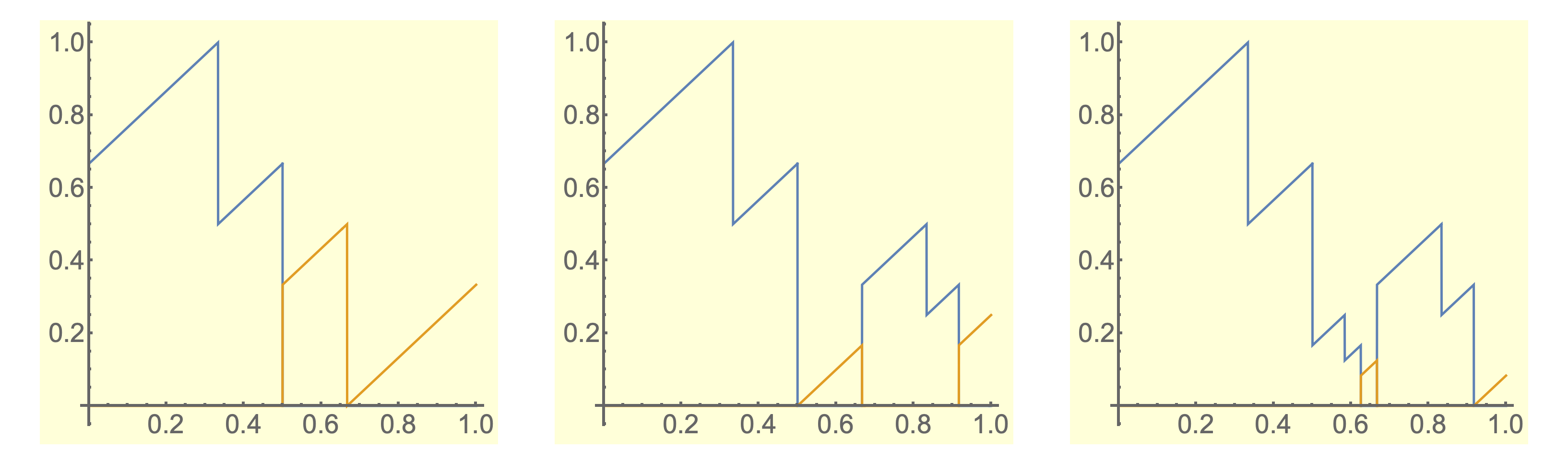
Figure 13. The graphs of $\displaystyle\mathfrak{F}_{1},\mathfrak{F}_{2},$ and $\displaystyle\mathfrak{F}_{3}$ for $\displaystyle\mathcal{S}_{PD}$

Although $\displaystyle\mathfrak{F}_{3}$ is only accurate on $\displaystyle 7/8$ of the interval, the pattern for filling in the remainder is visible from the progression. Moreover the refinements appear to provide the key to understanding the form of self-similarity taken.

4.2.1. Self-similarity of some $\displaystyle\mathfrak{F}$

All of the IIETs shown in this document exhibit repetitive properties that appear to be a form of self-similarity, perhaps via a graph-directed IFS. This reveals geometrically the self-inducing structure of $\displaystyle{\Sigma}$. The following result establishes self-similarity for a class of substitutions.

Proposition 4.9.

Suppose there are $\displaystyle\beta,\gamma\in{\mathcal{A}}$ such that $\displaystyle\mathcal{S}(\alpha)$ begins with $\displaystyle\beta$ and ends with $\displaystyle\gamma$ for all $\displaystyle\alpha\in{\mathcal{A}}$. Then there is a canonical IIET of $\displaystyle({\Sigma},\operatorname{\sigma},\mu)$ and a constant $\displaystyle\kappa\in[0,1)$ for which

(16) $$\mathfrak{F}(x)=\lambda(\mathfrak{F}(x/\lambda)+\kappa)\text{ for a.e. }x\in[0,1].$$

Proof.

Construct the initial partition $\displaystyle\mathcal{I}_{0}$ so that $\displaystyle{\mathbf{I}}(\gamma)=[0,\mu([\gamma]))$. No other restrictions on $\displaystyle\Phi_{0}$ are required.

Next, we need to choose $\displaystyle{\phi}$ (or $\displaystyle{\mathcal{S}_{*}}$). Since every supertile ends in a $\displaystyle\gamma$, we know $\displaystyle{\mathcal{S}_{*}}(\gamma)$ contains all of $\displaystyle{\mathcal{A}}$ and so we let $\displaystyle[0,1/\lambda)$ be partitioned the same way as $\displaystyle\mathcal{I}_{0}$ for these maximal supertiles. By similar logic we know that $\displaystyle{\mathcal{S}_{*}}(\beta)$ contains all of $\displaystyle{\mathcal{A}}$ and so we include a copy of $\displaystyle\mathcal{I}_{0}$ scaled by $\displaystyle\lambda$ in $\displaystyle{\mathbf{I}}(\beta)$ for these minimal supertiles. Denote this copy of $\displaystyle\mathcal{I}_{0}$ as $\displaystyle[\kappa,\kappa+1/\lambda)$ and note that $\displaystyle\kappa\in[1/\lambda,1)$.

Suppose the canonical isomorphism $\displaystyle\Phi$ and IIET $\displaystyle\mathfrak{F}$ have been constructed for this initial partition and refinement maps. We show that $\displaystyle\mathfrak{F}$ is self-similar.

The square $\displaystyle Q=[0,1/\lambda)\times[\kappa,\kappa+1/\lambda)$ contains all transitions from maximal 1-supertiles to minimal 1-supertiles. The maximal 1-supertiles that are not maximal 2-supertiles occupy the interval $\displaystyle[1/\lambda^{2},1/\lambda)$, and the transitions between them must be the same as the transitions between tiles within non-maximal supertiles. That means that if $\displaystyle x\in[1/\lambda^{2},1/\lambda)$, then $\displaystyle\mathfrak{F}(x)=\lambda^{-1}\mathfrak{F}(\lambda x)+\kappa$. Alternatively, if $\displaystyle x\in[1/\lambda,1)$, then $\displaystyle\mathfrak{F}(x)=\lambda(\mathfrak{F}(x/\lambda)-\kappa)$.

We prove the result inductively, extending it to $\displaystyle[1/\lambda^{2},1/\lambda)$ next. We know $\displaystyle[0,1/\lambda^{2})$ contains all the maximal 2-supertiles and will be mapped to the interval of length $\displaystyle 1/\lambda^{2}$ of minimal 2-supertiles, which begins at $\displaystyle\kappa(1+1/\lambda)$. The transitions between non-maximal 3-supertiles are the same as the transitions between non-maximal tiles within their supertiles, so

$$\mathfrak{F}(x)=\lambda^{-2}\mathfrak{F}(\lambda^{2}x)+\kappa(1+1/\lambda).$$

Since $\displaystyle\lambda^{2}x\in[1/\lambda,1)$, that means

$$\mathfrak{F}(\lambda^{2}x)=\lambda(\mathfrak{F}(\lambda^{2}x/\lambda)-\kappa)=\lambda(\mathfrak{F}(\lambda x)-\kappa).$$

Plugging into the expression for $\displaystyle\mathfrak{F}(x)$ yields

$$\mathfrak{F}(x)=\lambda^{-2}\left(\lambda(\mathfrak{F}(\lambda x)-\kappa)\right)+\kappa(1+1/\lambda)=\lambda^{-1}\mathfrak{F}(\lambda x)+\kappa.$$

Since $\displaystyle\lambda x\in[1/\lambda^{2},1/\lambda)$ this extends the result (16) to $\displaystyle[1/\lambda^{2},1)$. By induction we find the result to hold for all intervals of the form $\displaystyle[1/\lambda^{n},1)$. ∎

Remark 4.10.

Examples satisfying the proposition can be made with many known ergodic properties. The one shown in figure 14 has purely discrete dynamical spectrum.

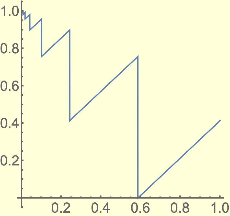
Figure 14. Shazam! A self-similar IIET for $\displaystyle A\to BBA,\,B\to BA$

5. Spectral analysis of $\displaystyle({\Sigma},\operatorname{\sigma},\mu)$

5.1. Review: spectral analysis in a general system (see e.g. [20, 18])

One way to study the behavior of a dynamical system $\displaystyle(X,T,\nu)$ is through the measurable functions it supports. It is particularly convenient to consider $\displaystyle L^{2}(X,\nu)$ because it is a Hilbert space. The function $\displaystyle h\in L^{2}(X,\nu)$ can be considered to be measuring some feature of each $\displaystyle x\in X$. If that feature repeats with some type of structure then $\displaystyle h$ may reveal it. A natural question is whether there is repetition under any powers of $\displaystyle T$, which leads to a Fourier analysis approach. The spectral coefficient $\displaystyle\hat{h}(j)$ is defined as the inner product

$$\hat{h}(j)=\left\langle T^{j}(h),\,h\right\rangle=\int_{X}h(T^{j}(x))\overline{h(x)}d\nu(x).$$

This expression compares the measurements $\displaystyle h$ takes at each pair $\displaystyle(x,T^{j}(x))$ and averages the result over all $\displaystyle x$. If there is significant structure in $\displaystyle(X,T)$ for $\displaystyle h$ to pick up, this will be reflected by larger values of $\displaystyle\hat{h}(j)$ for certain $\displaystyle j$s. It is well-known that the sequence of spectral coefficients is positive definite and so there is a spectral measure $\displaystyle z_{h}$ on the circle $\displaystyle S^{1}$ for which

$$\hat{h}(j)=\int_{S^{1}}z^{j}dz_{h}\quad\text{ for all }\quad j\in\mathbb{Z}.$$

An eigenfunction for $\displaystyle T$ is an $\displaystyle h\in L^{2}(X,\nu)$ for which there exists an eigenvalue $\displaystyle R\in\mathbb{R}$ with $\displaystyle h(T(x))=R\,h(x)$ for all $\displaystyle x\in X$. All constant functions are eigenfunctions and so it is customary to consider $\displaystyle h$ for which $\displaystyle\int_{X}h\,d\nu=0$ when looking at spectral measures.

5.2. The spectral measure of $\displaystyle\Phi$

In $\displaystyle\Phi$ we have an extraordinary function in $\displaystyle L^{2}({\Sigma},\mu)$. It measures the features of $\displaystyle\boldsymbol{\tau}\in{\Sigma}$ so accurately that it can almost always place it in a unique location in $\displaystyle[0,1]$. Moreover, that location is close to other $\displaystyle\boldsymbol{\tau}$s that strongly ‘resemble’ it as measured using any other test function in $\displaystyle L^{2}(X,\mu)$. Presumably this implies that the spectral measure of $\displaystyle\Phi$ is the maximal spectral type of the system.

For each $\displaystyle j\in\mathbb{Z}$ we compute the spectral coefficient using lemma 4.4

$$\hat{\Phi}(j)=\int_{\Sigma}\Phi(\operatorname{\sigma}^{j}(\boldsymbol{\tau}))\overline{\Phi(\boldsymbol{\tau})}\mu(d\boldsymbol{\tau})=\int_{0}^{1}\,x\,\mathfrak{F}^{j}(x)dx,$$

and since $\displaystyle\mathfrak{F}^{k}(x)=x+c_{i}$, where $\displaystyle c_{i}$ depends on the location of $\displaystyle x$, the integrand is a piecewise sum of upward-facing quadratics $\displaystyle x^{2}+c_{i}x$.

It is known [17] that shifting by sequences of the form $\displaystyle\{l_{n}=|\mathcal{S}^{n}(\alpha)|\}_{n=1}^{\infty}$ reveals the presence or absence of nonconstant eigenfunctions. Figures 15 through 19 in the discussions below exhibit a variety of behaviors of $\displaystyle\mathfrak{F}^{l_{n}}(x)$ for different substitutions, beginning with the constant-length case.

5.3. Special case: constant-length substitutions

The author believes there are variations of the following results that must hold for the general case, but the question remains open. For now we restrict ourselves to the well-studied special case.

We say $\displaystyle\mathcal{S}$ is a substitution of constant length if there is a $\displaystyle K\in\{2,3,...\}$ for which $\displaystyle|\mathcal{S}(\alpha)|=K$ for all $\displaystyle\alpha\in{\mathcal{A}}$. In this case $\displaystyle K$ is the expansion factor and all supertiles are of length $\displaystyle K^{n}$. The results in this section will not surprise you after looking at the comparison of relatively large powers of four examples with $\displaystyle K=2$ in figure 15.

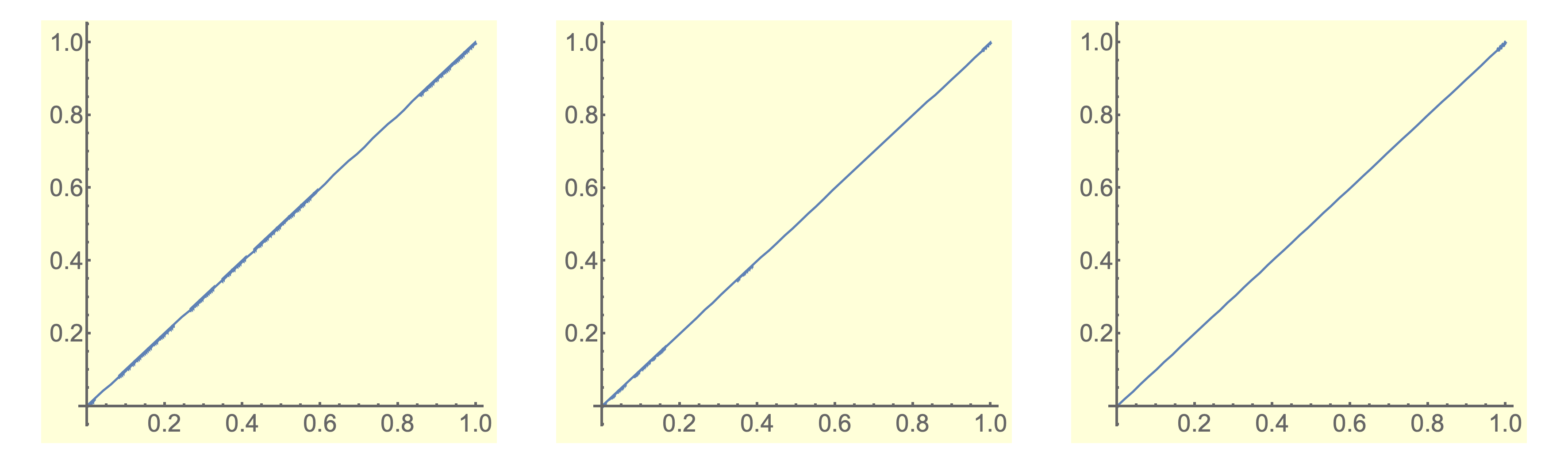
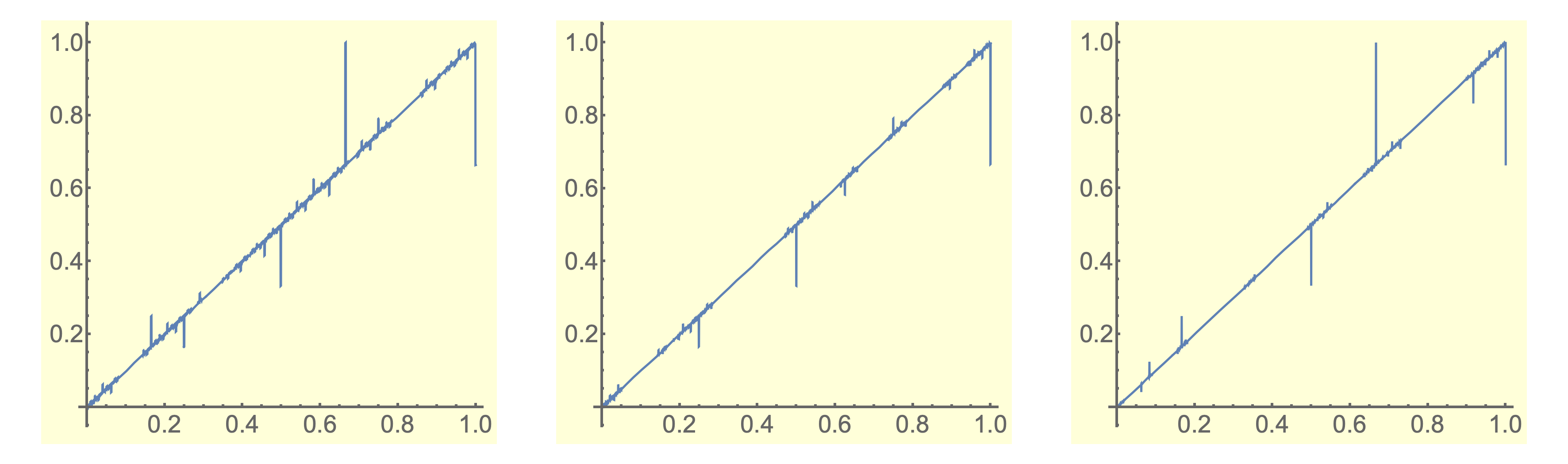
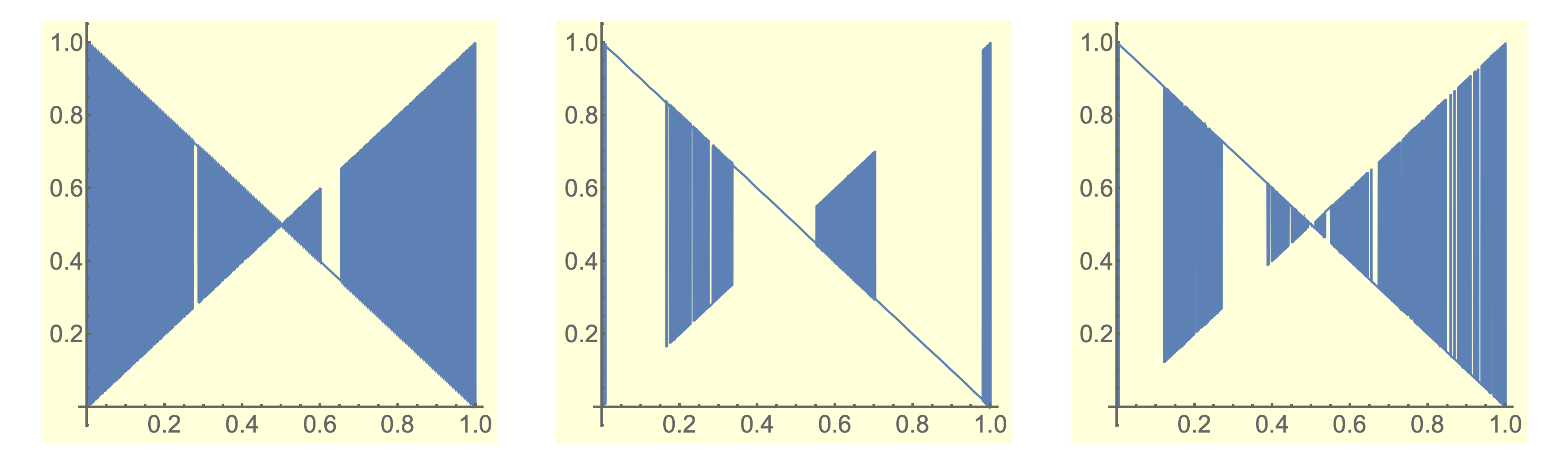
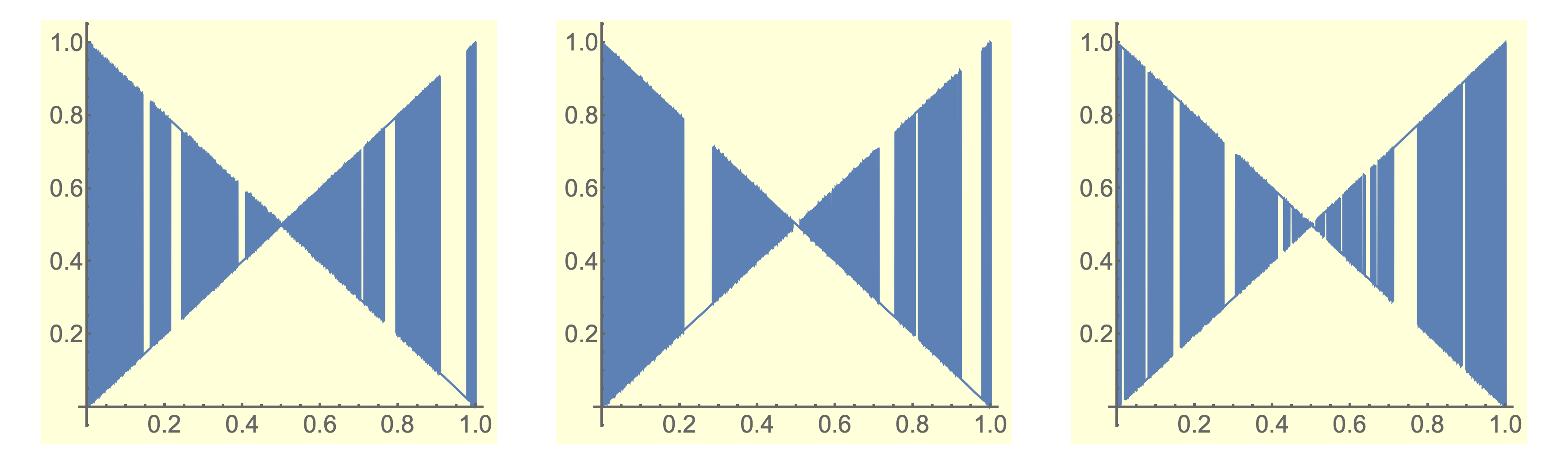
Figure 15. Rows are the 2-adic odometer, period-doubling, Thue–Morse, and Rudin–Shapiro IIETs. The graphs are $\displaystyle\mathfrak{F}_{20}^{j}$, where $\displaystyle j=2^{8},2^{9},$ and $\displaystyle 2^{10}$

Proposition 5.1.

If $\displaystyle\mathcal{S}$ is a primitive recognizable constant-length substitution with expansion factor $\displaystyle K$ then $\displaystyle\left\{\mathfrak{F}^{K^{n}}(x),\,n\in\mathbb{N}\right\}$ has at most $\displaystyle|{\mathcal{A}}|$ accumulation points for a.e. $\displaystyle x\in[0,1]$.

Proof.

Let $\displaystyle x$ be such that $\displaystyle\mathfrak{F}^{j}(x)$ is defined for all $\displaystyle j\in\mathbb{N}$. Choose $\displaystyle\boldsymbol{\tau}\in\Phi^{-1}(x)$ for which $\displaystyle{\boldsymbol{{\mathsf{a}}}}(x)={\boldsymbol{{\mathsf{a}}}}(\boldsymbol{\tau})$. Since $\displaystyle K^{n}$ is the length of an $\displaystyle n$-supertile, the $\displaystyle n$-supertile at the origin in $\displaystyle\operatorname{\sigma}^{K^{n}}(\boldsymbol{\tau})$ and in $\displaystyle\boldsymbol{\tau}$ are the same modulo $\displaystyle K^{n}$ but may be of different types. That makes $\displaystyle|{\mathcal{A}}|$ possible $\displaystyle n$-subintervals that could contain $\displaystyle\mathfrak{F}^{K^{n}}(x)$.

For $\displaystyle N>n$, $\displaystyle\boldsymbol{\tau}(0)$ and $\displaystyle\operatorname{\sigma}^{K^{N}}(\boldsymbol{\tau})(0)$ now are in the same position modulo $\displaystyle K^{N}$, so as before there are exactly $\displaystyle|{\mathcal{A}}|$ subintervals that could contain $\displaystyle\Phi(\operatorname{\sigma}^{K^{N}}(\boldsymbol{\tau}))$. Shifting by $\displaystyle K^{N}$ matches up $\displaystyle n$-supertiles as well, so the possible intervals for $\displaystyle\boldsymbol{\tau}$ and $\displaystyle\operatorname{\sigma}^{K^{N}}(\boldsymbol{\tau})$ are contained in the intervals for $\displaystyle\boldsymbol{\tau}$ and $\displaystyle\operatorname{\sigma}^{K^{n}}(\boldsymbol{\tau})$. Thus there are $\displaystyle|{\mathcal{A}}|$ nested sequences of intervals of vanishing length that $\displaystyle\mathfrak{F}^{K^{n}}(x)$ can visit as $\displaystyle n\to\infty$. The limits of their left endpoints are the possible accumulation points for $\displaystyle\left\{\mathfrak{F}^{K^{n}}(x),\,n\in\mathbb{N}\right\}$. ∎

The spectrum of constant-length substitutions is well-understood (see [11] and the survey [15]). The spectrum always contains $\displaystyle\mathbb{Z}[1/K]$, representing the underlying $\displaystyle K$-adic odometer structure. Questions of whether any other eigenfunctions, or any other significantly different functions at all, depends on how the letters populate the locations in $\displaystyle\mathcal{S}^{n}(\alpha)$ as $\displaystyle\alpha$ varies. A fundamental notion is the following.

Definition 5.2.

A substitution $\displaystyle\mathcal{S}$ has a coincidence if there are $\displaystyle N\in\mathbb{N},\beta\in{\mathcal{A}}$ and $\displaystyle j_{c}\in\{1,...,K^{N}\}$ such that $\displaystyle\beta$ is the $\displaystyle j_{c}$th letter of $\displaystyle\mathcal{S}^{N}(\alpha)$ for all $\displaystyle\alpha\in{\mathcal{A}}$. Elements in $\displaystyle\mathsf{A}$ of the form $\displaystyle(\alpha,j_{c})$ are called coincidence labels.

Theorem 5.3.

Let $\displaystyle\mathcal{S}$ be a primitive substitution of constant length $\displaystyle K>1$ with IIET $\displaystyle\mathfrak{F}$. Then $\displaystyle\lim_{n\to\infty}\mathfrak{F}^{K^{n}}(x)=x$ almost everywhere if and only if $\displaystyle\mathcal{S}$ has a coincidence.

Proof.

Suppose there is a coincidence, which by taking powers if necessary can be assumed to occur at $\displaystyle j_{c}\in\{1,...,K\}$. Consider $\displaystyle{\Sigma}_{c}$, the set of all $\displaystyle\boldsymbol{\tau}\in{\Sigma}$ such that $\displaystyle{\boldsymbol{{\mathsf{a}}}}(\boldsymbol{\tau})$ contains infinitely many coincidence labels. This is a set of full measure by lemma 4.1.

Let $\displaystyle x=\Phi(\boldsymbol{\tau})$ for $\displaystyle\boldsymbol{\tau}\in{\Sigma}_{c}$ and let $\displaystyle\epsilon>0$. Find some $\displaystyle n>1+|\ln(\epsilon)|$ at which $\displaystyle{\boldsymbol{{\mathsf{a}}}}(\boldsymbol{\tau})$ has a coincidence label. Then $\displaystyle{\boldsymbol{{\mathsf{a}}}}_{{n-1}}(\boldsymbol{\tau})$ is the same no matter what the type $\displaystyle\pi_{\mathcal{A}}({\mathsf{a}}_{n})$. Any shift of $\displaystyle\boldsymbol{\tau}$ by $\displaystyle K^{N}$ where $\displaystyle N>n$ aligns the $\displaystyle n$-supertiles, so $\displaystyle{\boldsymbol{{\mathsf{a}}}}(\operatorname{\sigma}^{K^{N}}(\boldsymbol{\tau}))$ also has a coincidence label at $\displaystyle n$. That is, $\displaystyle\boldsymbol{\tau}(0)$ and $\displaystyle(\operatorname{\sigma}^{K^{N}}(\boldsymbol{\tau}))(0)$ are in the same $\displaystyle n-1$ supertile in the same location. Their images under $\displaystyle\Phi$ must both be in $\displaystyle{\mathbf{I}}({\boldsymbol{{\mathsf{a}}}}_{{n-1}}(\boldsymbol{\tau}))$ which has length $\displaystyle=1/K^{n-1}<\epsilon$. This shows $\displaystyle\mathfrak{F}^{K^{n}}(x)\to x$ for any $\displaystyle x\in\Phi({\Sigma}_{c})$.

Now suppose $\displaystyle\lim_{n\to\infty}\mathfrak{F}^{K^{n}}(x)=x$ almost everywhere and let $\displaystyle\delta>0$ such that $\displaystyle\delta<\mu([\alpha\beta])$ for all legal two-letter words $\displaystyle\alpha\beta$. By Egorov’s theorem there is a set $\displaystyle{D_{\delta}}\subset[0,1]$ on which the convergence is uniform and $\displaystyle m({D_{\delta}})\geq 1-\delta$. Choose $\displaystyle M$ so that if $\displaystyle n\geq M$ then $\displaystyle|\mathfrak{F}^{K^{M}}(x)-x|<\delta$ for all $\displaystyle x\in{D_{\delta}}$.

Let $\displaystyle{E}(j)$ be the set of all sequences in the $\displaystyle j$th spot of their $\displaystyle M$ supertile, i.e.

$${E}(j)=\bigcup_{\alpha\in{\mathcal{A}}}\operatorname{\sigma}^{j}(\mathcal{S}^{M}([\alpha)]),$$

which has measure $\displaystyle\mu({E}(j))=1/K^{M}$. Let $\displaystyle{E_{\delta}}(j)={E}(j)\cap{D_{\delta}}$. Let $\displaystyle j_{c}$ be the index for which $\displaystyle\mu({E_{\delta}}(j))\leq\mu({E_{\delta}}(j_{c}))$ for all $\displaystyle j\in\{1,...,K^{M}\}$. We claim $\displaystyle j_{c}$ is a coincidence for $\displaystyle\mathcal{S}$.

For the sake of contradiction suppose there are $\displaystyle\hat{\alpha}$ and $\displaystyle\hat{\beta}$ that differ at their $\displaystyle j_{c}$th spot: $\displaystyle\mathcal{S}^{M}(\hat{\alpha})_{j_{c}}\neq\mathcal{S}^{M}(\hat{\beta})_{j_{c}}$. Then $\displaystyle\operatorname{\sigma}^{j_{c}}(\mathcal{S}^{M}([\hat{\alpha}\hat{\beta}]))\notin{E_{\delta}}$, since $\displaystyle\boldsymbol{\tau}$ and $\displaystyle\operatorname{\sigma}^{j_{c}}(\boldsymbol{\tau})$ are not within $\displaystyle\delta$ of one another for any $\displaystyle\boldsymbol{\tau}$ it contains. That means $\displaystyle\mu({E_{\delta}}(j_{c}))\leq\mu({E}(j_{c}))-\mu(\operatorname{\sigma}^{j_{c}}([\hat{\alpha}\hat{\beta}]))=1/K^{M}-\mu([\hat{\alpha}\hat{\beta}]))/K^{M}.$ Since $\displaystyle\mu({E_{\delta}}(j_{c}))$ is the maximum measure over the $\displaystyle j$s we see that

$$\mu({E_{\delta}})=\sum_{j=1}^{K^{M}}\mu({E_{\delta}}(j))\leq K^{M}\mu({E_{\delta}}(j_{c}))\leq 1-\mu([\hat{\alpha}\hat{\beta}])<1-\delta.$$

Since $\displaystyle\mu({E_{\delta}})=m({D_{\delta}})$, this contradicts the definition of $\displaystyle{D_{\delta}}$ and completes the proof. ∎

5.4. Pictures for the non-constant length case.

The author had originally posited a connection between having purely discrete spectrum and some type of convergence of $\displaystyle\mathfrak{F}^{l_{n}}(x)$ to the identity. This problem is closely connected to the Pisot substitution conjecture [2]. The next few figures show shifts by large supertile amounts for some familiar examples.

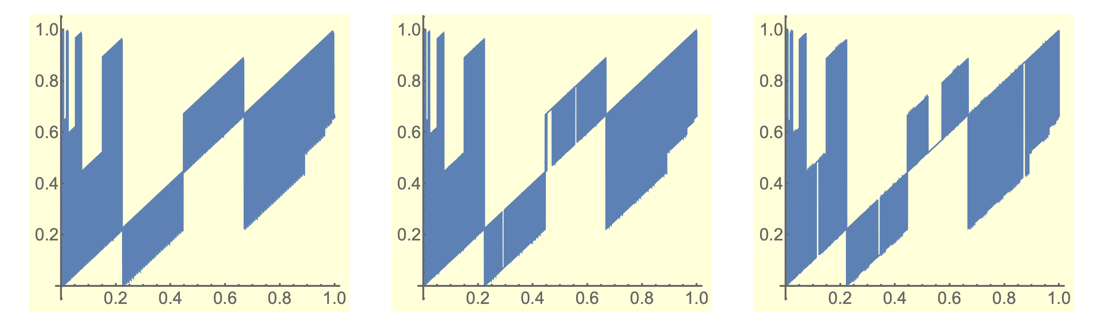
Figure 16. The IIET $\displaystyle\mathfrak{F}_{20}^{j}$ for the Chacon substitution $\displaystyle\mathcal{S}_{C}(0)=0\,0\,1\,0$ and $\displaystyle\mathcal{S}_{C}(1)=1$, where $\displaystyle j=121,j=364,$ and $\displaystyle j=1093$. The subshift is uniquely ergodic and weakly mixing

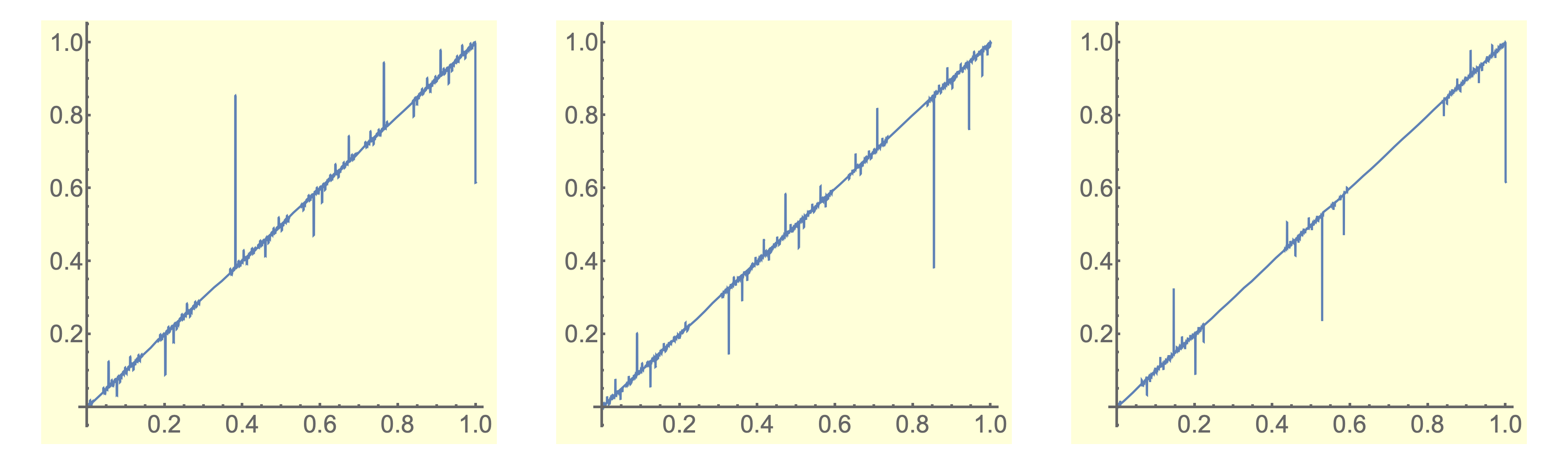
Figure 17. Fibonacci IIET $\displaystyle\mathfrak{F}_{30}^{j}$, where $\displaystyle j=377,j=610,$ and $\displaystyle j=987$

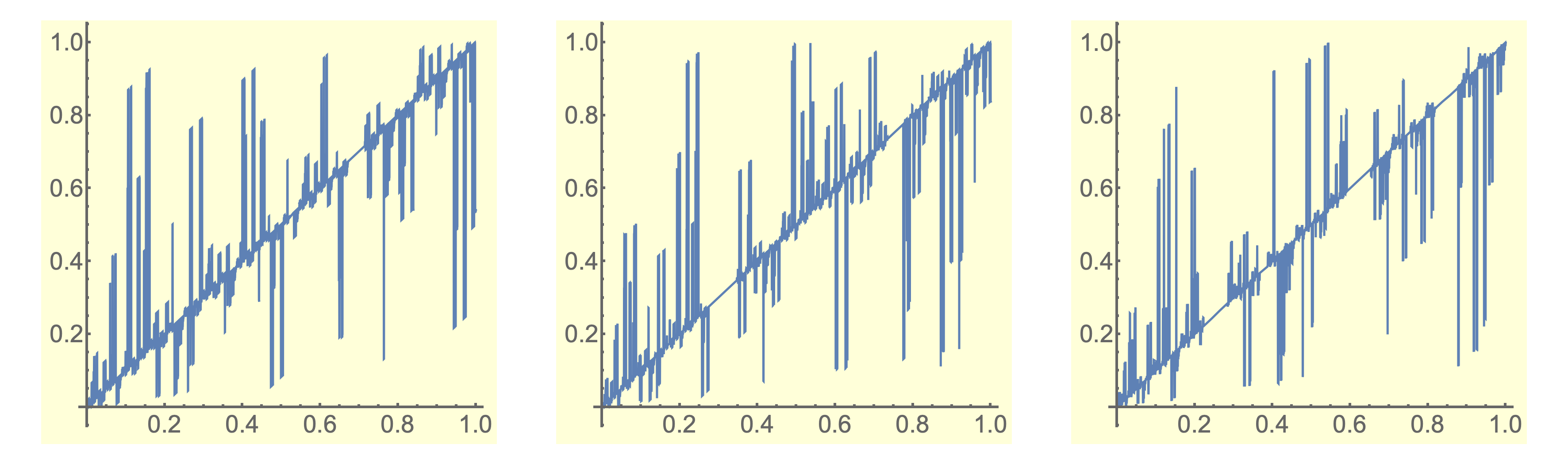
Figure 18. The IIET $\displaystyle\mathfrak{F}_{20}^{j}$ for the tribonacci substitution $\displaystyle A\to AB,\,B\to AC,\,C\to A$, for $\displaystyle j=204,j=574,$ and $\displaystyle j=927$

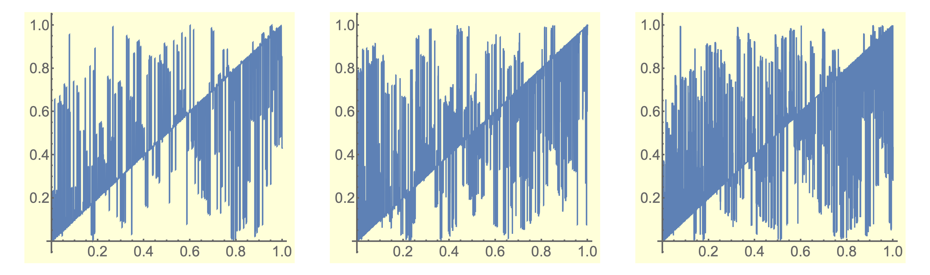
Figure 19. The IIET $\displaystyle\mathfrak{F}_{20}^{j}$ for the substitution $\displaystyle A\to ABBB,\,B\to A$, for $\displaystyle j=217,j=508,$ and $\displaystyle j=1159$. This substitution has some singular continuous spectrum [5]

6. Self-similar tilings, S-adic sequences and fusion tilings of $\displaystyle\mathbb{R}$

Our construction works in a number of other situations. We provide a relatively complete description of the one-dimensional case below. Preliminary work is being carried out in higher dimensions[16]. For subshifts in $\displaystyle\mathbb{Z}^{m}$ the result is $\displaystyle m$ commuting IIETs on $\displaystyle[0,1]$, and for fusion tilings there is a canonical flow view representation but the action of the first return map is less clear.

6.1. S-adic systems

These systems are generated with substitutions that can vary at each level. A general S-adic system is generated by a directive sequence of morphisms $\displaystyle\mathcal{S}_{n}:{\mathcal{A}}_{n}\to{\mathcal{A}}_{n-1}^{+}$ on a sequence $\displaystyle{\mathcal{A}}_{0},{\mathcal{A}}_{1},{\mathcal{A}}_{2},{\mathcal{A}}_{3},...$ of finite alphabets. The $\displaystyle n$-supertiles are of the form $\displaystyle\mathcal{S}_{1}(\mathcal{S}_{2}(...(\mathcal{S}_{n}(\alpha))...)$, where $\displaystyle\alpha\in{\mathcal{A}}_{n}$, and a subshift of all admissible sequences is obtained as in definition 2.2. A classic type of S-adic system is made by taking all substitutions with a given transition matrix $\displaystyle M$ on a single alphabet $\displaystyle{\mathcal{A}}$. In that situation the estimates from corollary 4.8 still hold, and a single dual substitution can be chosen to construct the flow view.

For S-adic symbolic systems the notion of recognizability (along with other things) becomes more nuanced [7]. We assume the strongest form: full recognizability, where each substitution in the directive sequence is recognizable. We also assume that the subshift admitted by the supertiles is minimal. In this case there is no direct Perron-Frobenius theorem to give us information about the natural lengths or frequencies. However, there is a sequence of transition matrices and that any invariant measure for the subshift must obey a type of transition-consistency that forces the left equation of (6) to be true at each level.

There are two adaptations needed to our proof. First, we need an address set $\displaystyle\mathsf{A}_{n}$ for each $\displaystyle\mathcal{S}_{n}$, constructed as before (4). Addresses for $\displaystyle n$-cylinders will be those elements of $\displaystyle\mathsf{A}_{1}\times\mathsf{A}_{2}\times...\times\mathsf{A}_{n}$ that represent allowable supertile inclusions. The refining sequence $\displaystyle\{\mathcal{B}_{n}\}$ of $\displaystyle{\Sigma}$ is canonical, as is the order on the Bratteli diagram. The second adaptation is to produce a new $\displaystyle{\phi}$ function at each level. Because the measure is transition-consistent, we can partition the intervals for $\displaystyle n$-supertiles into the subintervals corresponding to their $\displaystyle(n+1)$-tiles and define $\displaystyle{\phi}_{n}$ with them as in equation (7). As before, some initial partition using the alphabet $\displaystyle{\mathcal{A}}_{0}$ on which the sequence space is based is required to make $\displaystyle\Phi_{0}$. Equation (8) becomes

(17) $${\Phi}_{n}({\boldsymbol{{\mathsf{a}}}})={\Phi}_{n-1}({\mathsf{a}}_{1}\,...,{\mathsf{a}}_{n-1})+{\phi}_{n}({\mathsf{a}}_{n}).$$

The rest of the proofs are made with these adaptations.

6.2. Tilings of $\displaystyle\mathbb{R}$

Self-similar and fusion tilings of $\displaystyle\mathbb{R}$ are suspensions of substitution and S-adic systems, respectively, and in this case it is the first return map to a transversal that is conjugate to the IIET. The height function is given by a choice lengths of the tiles, and to compare their systems they need to be normalized. The right eigenvector controls the measure and cannot be changed. In the symbolic case we already have that $\displaystyle\vec{r}$ is a probability and the length vector is all ones. Thus for the natural lengths we should choose the left eigenvector for which $\displaystyle\vec{l}\cdot\vec{r}=1$. Flow views below are scaled properly.

Example 6.1.

Figure 20 shows the flow views for the tribonacci substitution ($\displaystyle A\to AB,\,B\to AC,\,C\to A$) first as unit tiles and then as its suspension using the normalized natural tile lengths.

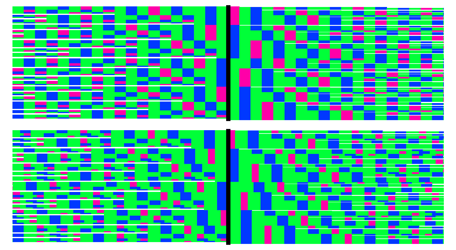
Figure 20. Flow views for the tribonacci substitution. Top: unit length tiles. Bottom: natural length tiles. For the tiling flow, the IIET is the first return map to the transversal of all tilings with an endpoint at 0

Any appropriately scaled suspensions over the tribonacci substitution are topologically conjugate to one another as tiling flows [10]. The conjugacy is non-local, exemplifying the fact that tiling flows do not have a Curtis-Lyndon-Hedlund theorem. $\displaystyle\Diamond$

Example 6.2.

Figure 21 shows the flow views for the well-studied non-Pisot substitution rule $\displaystyle A\to ABBB,\,B\to A$. Powers of its IIET were shown in figure 19.

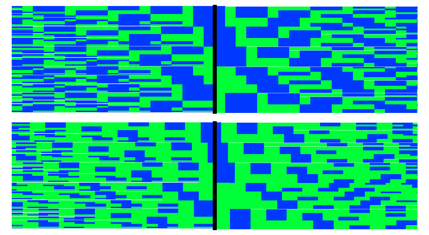
Figure 21. Flow views for $\displaystyle A\to ABBB,\,,B\to A$. Top: unit tiles. Bottom: natural length, properly scaled

This substitution has two distinct eigenvalues of large modulus. Again from [10] we know that even when properly normalized, the tiling flows are not topologically conjugate unless the tile lengths are rationally related. The two flows shown are not conjugate. $\displaystyle\Diamond$

Example 6.3 (Chacon substitution).

The Chacon substitution $\displaystyle\mathcal{S}_{C}(0)=0\,0\,1\,0$ and $\displaystyle\mathcal{S}_{C}(1)=1$ is not primitive, but it is minimal and uniquely ergodic and therefore its subshift has canonical IIETs.

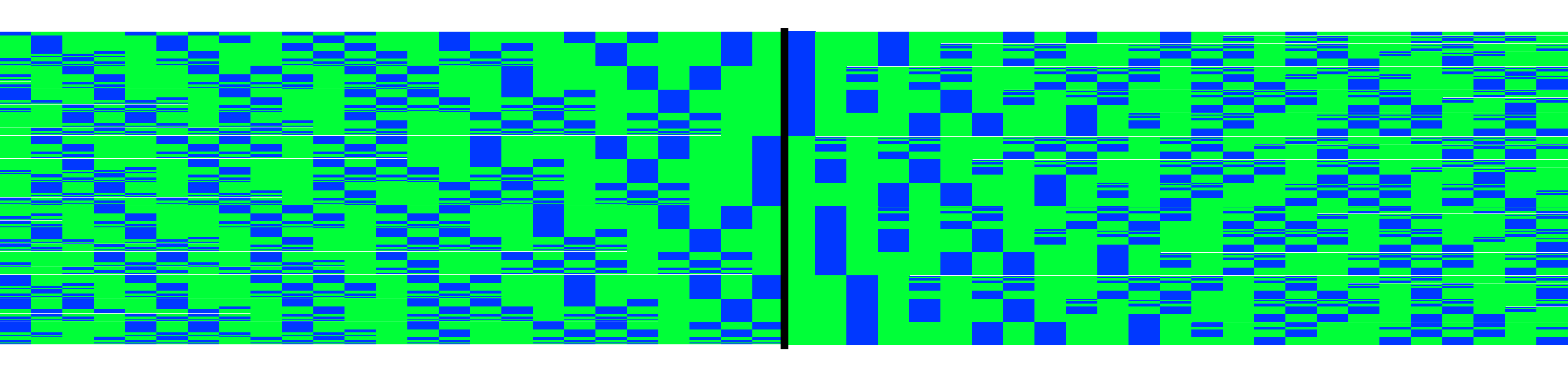
Figure 22. There is no meaningful natural length flow view to compare to the Chacon substitution subshift

The lack of primitivity prohibits a representative flow view for the natural length tiles. The natural length for “$\displaystyle 1$” is 0, so the result is a 3-odometer on just the $\displaystyle 0$ tile. Its flow view would look like a solid green rectangle, so only the unit length flow view is pictured in figure 22. $\displaystyle\Diamond$

7. Questions, comments, observations

The author has fallen down numerous rabbit holes of high (to her) entertainment value. The following is a somewhat random assortment of her favorites.

✤ Any substitution whose subshift is minimal and recognizable has numerous IIET/flow view combinations that represent it. In the simplest case we could consider only the set of canonical IIETs given by all possible dual substitutions. This produces a finite list of $\displaystyle(\Phi_{j},\mathfrak{F}_{j})$s that all represent $\displaystyle({\Sigma},\operatorname{\sigma},\mu)$.

• What information is contained in the measure-theoretic automorphisms $\displaystyle\Phi_{2}^{-1}\circ\Phi_{1}$ of $\displaystyle{\Sigma}$?

• Many substitutions have a periodic dual substitution which, if treated as recognizable, would be an odometer. What is the significance of this?

• Is there an optimal choice of dual substitution to represent a system?

✤ The flow view construction provides a link between all substitutions and S-adic systems that share a common primitive transition matrix $\displaystyle M$.

• For any given substitution, an S-adic system using any or all of the choices of dual substitution could be used, in which case the representation would be non-canonical.

• Alternatively, S-adic systems in which the directive sequence shares a transition matrix can be modeled with a dual substitution for its flow view.

• Take two subshifts with coordinate maps given by the same dual substitution. This gives a measure-theoretic bijection between the subshifts. How do the properties of the matrix affect the properties of this bijection?

✤ The Fibonacci substitution subshift is known to correspond to an exchange of two intervals, but the $\displaystyle\mathfrak{F}$ that appears in figure 1 of our introduction exchanges infinitely many. That’s because there are only two choices of dual substitution for $\displaystyle\mathcal{S}_{fib}$, and both yield exchanges of infinitely many intervals. There are two main ways to enlarge the scope. One is to allow all canonical $\displaystyle(\Phi_{j},\mathfrak{F}_{j})$s for all powers of the substitution. The other is to allow the subdivisions to vary at each stage, producing an S-adic subdivisions. The latter has not been investigated so far, but the former allows the Fibonacci two-interval exchange to appear from our process. With $\displaystyle\mathcal{S}_{fib}^{2}$ and the correct choice of dual substitution, figure 23 shows how the approximants become the two-interval exchange.

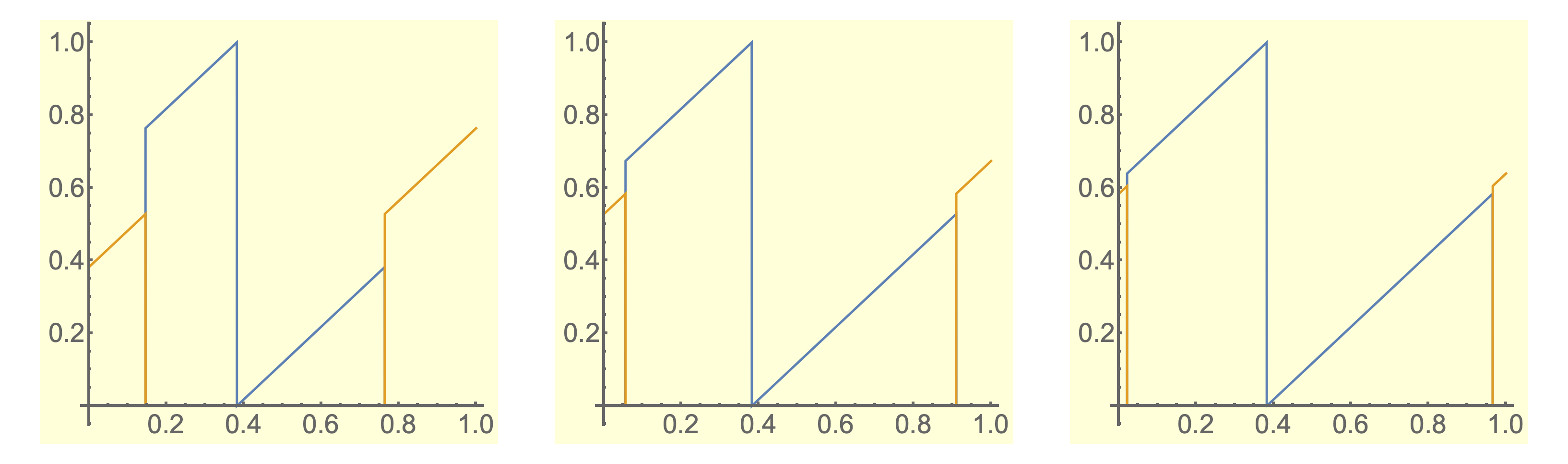
Figure 23. The first three approximants for the IIET of $\displaystyle\mathcal{S}_{fib}^{2}$

• Conjecture: If a substitution subshift is measurably conjugate to a finite interval exchange transformation, that transformation is a member of the family of canonical infinite interval exchange transformations of its powers.

• One can define the efficiency of an IIET representation in terms of how many total translations/intervals are possible given the size of the substitution versus how many the IIET actually needs. For instance, since the Fibonacci subshift can be represented with an IET of two intervals, the efficiency of any other canonical representation can be compared. In general this is expected to require asymptotic analysis.

✤ The destination under $\displaystyle\Phi$ of a randomly selected tiling is ‘expected’ to be $\displaystyle\int_{\Sigma}\Phi(\boldsymbol{\tau})d\mu=\int_{0}^{1}x\,dx=1/2$. This indicates that $\displaystyle\boldsymbol{\tau}\in\Phi^{-1}(1/2)$ might be particularly representative examples. The stability and other properties of this set under choice of dual substitution is not yet known.

✤ In [9], the authors begin with the dyadic odometer as an IIET and then ‘twist’ it, obtaining new translation surfaces encoding, eventually, S-adic or substitution subshifts as minimal components. Remarkably, a power of the Fibonacci substitution appears as a minimal component and does not have the odometer as a factor [9, Section 5.4].

• The method is a sort of inverse of the one in this paper, beginning with an IIET and ending with a subshift. To what degree can the two together classify the IIETs of self-inducing subshifts?

• Can our method ‘find’ the dyadic odometer for the Fibonacci substitution? If so can it find other, perhaps Fibonacci-number-adic, odometers?

References

- [1] S. Akiyama and P. Arnoux. Substitution and Tiling Dynamics: Introduction to Self-inducing Structures: CIRM Jean-Morlet Chair, Fall 2017. Lecture Notes in Mathematics. Springer International Publishing, 2020.
- [2] S. Akiyama, M. Barge, V. Berthé, J.-Y. Lee, and A. Siegel. On the Pisot substitution conjecture. In Mathematics of aperiodic order, volume 309 of Progr. Math., pages 33–72. Birkhäuser/Springer, Basel, 2015.
- [3] P. Arnoux and A. M. Fisher. The scenery flow for geometric structures on the torus: the linear setting. Chinese Ann. Math. Ser. B, 22(4):427–470, 2001.
- [4] Pierre Arnoux, Donald S. Ornstein, and Benjamin Weiss. Cutting and stacking, interval exchanges and geometric models. Israel J. Math., 50(1-2):160–168, 1985.
- [5] Michael Baake, Natalie Priebe Frank, Uwe Grimm, and E. Arthur Robinson, Jr. Geometric properties of a binary non-Pisot inflation and absence of absolutely continuous diffraction. Studia Math., 247(2):109–154, 2019.
- [6] Valérie Berthé and Anne Siegel. Tilings associated with beta-numeration and substitutions. Integers, 5(3):A2, 46, 2005.
- [7] Valérie Berthé, Wolfgang Steiner, Jörg M. Thuswaldner, and Reem Yassawi. Recognizability for sequences of morphisms. Ergodic Theory Dynam. Systems, 39(11):2896–2931, 2019.
- [8] S. Bezuglyi and O. Karpel. Bratteli diagrams: structure, measures, dynamics. In Dynamics and numbers, volume 669 of Contemp. Math., pages 1–36. Amer. Math. Soc., Providence, RI, 2016.
- [9] Henk Bruin and Olga Lukina. Rotated odometers, 2021.
- [10] Alex Clark and Lorenzo Sadun. When size matters: subshifts and their related tiling spaces. Ergodic Theory Dynam. Systems, 23(4):1043–1057, 2003.
- [11] F. M. Dekking. The spectrum of dynamical systems arising from substitutions of constant length. Z. Wahrscheinlichkeitstheorie und Verw. Gebiete, 41(3):221–239, 1977/78.
- [12] Tomasz Downarowicz and Alejandro Maass. Finite-rank Bratteli-Vershik diagrams are expansive. Ergodic Theory Dynam. Systems, 28(3):739–747, 2008.
- [13] Jean-Marie Dumont and Alain Thomas. Systemes de numeration et fonctions fractales relatifs aux substitutions. Theoret. Comput. Sci., 65(2):153–169, 1989.
- [14] F. Durand, B. Host, and C. Skau. Substitutional dynamical systems, Bratteli diagrams and dimension groups. Ergodic Theory Dynam. Systems, 19(4):953–993, 1999.
- [15] N. Pytheas Fogg. Substitutions in dynamics, arithmetics and combinatorics, volume 1794 of Lecture Notes in Mathematics. Springer-Verlag, Berlin, 2002. Edited by V. Berthé, S. Ferenczi, C. Mauduit and A. Siegel.
- [16] Natalie Priebe Frank and Lorenzo Sadun. In progress, 2021.
- [17] B. Host. Valeurs propres des systèmes dynamiques définis par des substitutions de longueur variable. Ergodic Theory Dynam. Systems, 6(4):529–540, 1986.
- [18] Anatole Katok and Jean-Paul Thouvenot. Spectral properties and combinatorial constructions in ergodic theory. In Handbook of dynamical systems. Vol. 1B, pages 649–743. Elsevier B. V., Amsterdam, 2006.
- [19] Bruce P. Kitchens. Symbolic dynamics. Universitext. Springer-Verlag, Berlin, 1998. One-sided, two-sided and countable state Markov shifts.
- [20] Karl Petersen. Ergodic theory, volume 2 of Cambridge Studies in Advanced Mathematics. Cambridge University Press, Cambridge, 1989. Corrected reprint of the 1983 original.
- [21] Martine Queffélec. Substitution dynamical systems—spectral analysis, volume 1294 of Lecture Notes in Mathematics. Springer-Verlag, Berlin, second edition, 2010.