$\boldsymbol{S}$-dual Inflation and the String Swampland

Abstract

The Swampland de Sitter conjecture in combination with upper limits on the tensor-to-scalar ratio $r$ derived from observations of the cosmic microwave background endangers the paradigm of slow-roll single field inflation. This conjecture constrains the first and the second derivatives of the inflationary potential in terms of two ${\cal O}(1)$ constants $c$ and $c^{\prime}$. In view of these restrictions we reexamine single-field inflationary potentials with $S$-duality symmetry, which ameliorate the unlikeliness problem of the initial condition. We compute $r$ at next-to-leading order in slow-roll parameters for the most general form of $S$-dual potentials and confront model predictions to constraints imposed by the de Sitter conjecture. We find that $c\sim{\cal O}(10^{-1})$ and $c^{\prime}\sim{\cal O}(10^{-2})$ can accommodate the 95% CL upper limit on $r$. By imposing at least 50 $e$-folds of inflation with the effective field theory description only valid over a field displacement ${\cal O}(1)$ when measured as a distance in the target space geometry, we further restrict $c\sim{\cal O}(10^{-2})$, while the constraint on $c^{\prime}$ remains unchanged. We comment on how to accommodate the required small values of $c$ and $c^{\prime}$.

I Introduction

Inflation is the leading paradigm for explaining the behavior of the quasi-de Sitter expansion in the very early universe. Single-field inflationary models provide promising explanations to the cosmological horizon problem, the lack of topological defects, and the observed large-scale isotropy Guth:1980zm ; Linde:1981mu ; Albrecht:1982wi . In addition, inflation provides a mechanism for generating small fluctuations in energy density, which could have seeded galactic structure formation Mukhanov:1981xt ; Hawking:1982cz ; Guth:1982ec ; Starobinsky:1982ee ; Bardeen:1983qw , and are observed in the temperature anisotropies of the cosmic microwave background (CMB) Spergel:2003cb ; Komatsu:2010fb .

One of the main goals of modern CMB missions is to measure the tensor-to-scalar ratio $r$ accurately to constrain inflationary models. The combination of BICEP2/Keck Array data with observations by Planck (TT,TE,EE +lowE+lensing) and BAO significantly shrink the space of allowed inflationary cosmologies: $r<0.068$ at 95% CL Ade:2018gkx ; Akrami:2018odb . Moreover, CMB data favor standard slow-roll single field inflationary models with plateau-like potentials $V$, for which $V_{\phi\phi}<0$, over power-law potentials; here $\phi$ is the dilaton/inflaton and $V_{\phi}\equiv dV/d\phi$ Ade:2015lrj . In this paper we investigate slow-roll inflationary models within the context of the Swampland program Vafa:2005ui and confront model predictions with experiment. We particularize the investigation to inflationary potentials satisfying $V_{\phi\phi}<0$ while being invariant under the $S$-duality constraint, $\phi\rightarrow-\phi$ Montonen:1977sn , which is reminiscent of String Theory Font:1990gx ; Sen:1994fa .

The Swampland program has been established to lay out a connection between quantum gravity and very-large-scale/ultra-low-energy astronomical observations. The String Swampland comprises the set of (apparently) consistent effective field theories (EFT) that cannot be completed into quantum gravity in the ultraviolet Brennan:2017rbf ; Palti:2019pca . This rather abstract concept implies that if gravity were to be added into an EFT which is self-consistent up to a scale $E_{\rm self}$, then the combined theory would exhibit a new limitting energy scale $E_{\rm swamp}$, above which the theory must be modified if it is to become compatible with quantum gravity in the ultraviolet. When the energy relation $E_{\rm swamp}<E_{\rm self}<E_{\rm Pl}$ holds and $E_{\rm swamp}$ is below any characteristic energy scale involved in the theory, we say that the entire EFT belongs to the String Swampland; $E_{\rm Pl}$ denotes the Planck energy scale. Guidance for a model building approach is provided by an ensemble of Swampland conjectures ArkaniHamed:2006dz ; Ooguri:2006in ; Klaewer:2016kiy ; Ooguri:2018wrx ; Grimm:2018ohb ; Heidenreich:2018kpg ; Ooguri:2016pdq ; Palti:2017elp ; Obied:2018sgi ; Andriot:2018wzk ; Kehagias:2018uem ; Cecotti:2018ufg ; Klaewer:2018yxi ; Heckman:2019bzm ; Lust:2019zwm ; Bedroya:2019snp ; Kehagias:2019akr ; Blumenhagen:2019vgj ; Andriot:2020lea ; Gendler:2020dfp ; Bonnefoy:2020uef ; Perlmutter:2020buo ; Luben:2020wix ; Calderon-Infante:2020dhm ; Kolb:2021xfn . There are two consequential conjectures which gathered immediate interest in the context of inflationary cosmology:

• Distance Swampland conjecture: This conjecture limits the field space of validity of any EFT by limiting the field excursion $\Delta\phi$ to be small when expressed in Planck units, namely $\Delta\phi/M_{\rm Pl}\equiv\delta\lesssim\alpha\sim{\cal O}(1)$, where $M_{\rm Pl}=(8\pi G)^{-1/2}$ is the reduced Planck mass Ooguri:2006in ; Klaewer:2016kiy ; Ooguri:2018wrx ; Grimm:2018ohb ; Heidenreich:2018kpg .

• de Sitter conjecture: The gradient of the scalar potential $V$ must satisfy the lower bound,

  $$M_{\rm Pl}\frac{|V_{\phi}|}{V}\equiv{\cal C}\geq c\,,$$ (1)

  or else its Hessian must satisfy

  $$M_{\rm Pl}^{2}\frac{V_{\phi\phi}}{V}\equiv{\cal C^{\prime}}\leq-c^{\prime}$$ (2)

  where $c$ and $c^{\prime}$ are positive order-one numbers in Planck units Obied:2018sgi ; Ooguri:2018wrx .

It has been noted that while the distance conjecture by itself does not pose significant challenge for single-field inflationary models (and corresponds observationally to a suppressed $r$ through the well-known Lyth bound Lyth:1996im ), the de Sitter conjecture is in direct tension with slow-roll inflationary potentials favored by CMB data Agrawal:2018own ; Achucarro:2018vey ; Garg:2018reu ; Ben-Dayan:2018mhe ; Kinney:2018nny ; Fukuda:2018haz ; Garg:2018zdg ; Agrawal:2018rcg ; Chiang:2018lqx . The objective of our investigation is to analyze the status of single-field inflationary potentials with $S$-duality symmetry in the context of the Swampland conjectures.

The remainder of the paper is structured as follows. In Sec. II we first provide an overview of the equations of motion in single-field slow-roll inflation and introduce the definition of the slow-roll parameters. After that, to make the connection with experiment we compute the scalar spectral index $n_{s}$ and the tensor-to-scalar ratio $r$ at next-to-leading order (NLO) in slow-roll parameters. In Sec. III we examine the subtleties of model building while imposing contraints which depend on multiple slow-roll parameters focussing attention on $S$-dual symmetric inflationary potentials. We summarize the generalities of these potentials and confront model predictions to the CMB observables $n_{s}$ and $r$. In Sec. IV we investigate the ambiguity on the definition of the slow-roll parameters and explore whether this uncertainty can help ameliorate the tension between single-field inflationary models and the de Sitter Swampland conjecture. The paper wraps up with some conclusions presented in Sec. V.

II Constraints on $\boldsymbol{r}$ at NLO in slow-roll parameters

The essential property of nearly all crowned inflationary models is a period of slow-roll evolution of $\phi$ during which its kinetic energy remains always much smaller than its potential energy. The equation of motion for the canonical homogeneous inflaton field is

$$\ddot{\phi}+3H\dot{\phi}+V_{\phi}=0\,,$$ (3)

where $H=\dot{a}/a$ is the Hubble parameter and dot denotes derivative with respect to the cosmic time. The slow-roll conditions

$${\textstyle\frac{1}{2}}\dot{\phi}^{2}\ll|V|$$ (4)

and

$$\left|\frac{\ddot{\phi}}{3H\dot{\phi}}\right|\ll 1\,,$$ (5)

imply

$$\epsilon\equiv\frac{M_{\rm Pl}^{2}}{2}\left(\frac{V_{\phi}}{V}\right)^{2}\ll 1$$ (6)

and

$$\eta\equiv M_{\rm Pl}^{2}\left[\frac{V_{\phi\phi}}{V}-\frac{1}{2}\left(\frac{V_{\phi}}{V}\right)^{2}\right]\ll 1\,,$$ (7)

respectively Kolb:1994ur ; Dodelson:1997hr . The Friedmann relation incorporating slow-roll is given by

$$H(\phi)\simeq\sqrt{\frac{V}{3M_{\rm Pl}^{2}}}\,.$$ (8)

At the end of slow roll, $\phi$ falls into the core of the potential and oscillates rapidly around the minimum, ultimately leading to the reheating period. The amount of inflationary expansion within a given timescale is generally parametrized in terms of the number of $e$-foldings that occur as the scalar field rolls from a particular value $\phi$ to its value $\phi_{e}$ when inflation ends:

$$N(\phi\to\phi_{e})=-\frac{1}{M_{\rm Pl}^{2}}\int_{\phi}^{\phi_{e}}\frac{V}{V_{\phi}}d\phi\,,$$ (9)

with ${\epsilon}(\phi_{e})=1$ Remmen:2014mia . The de Sitter conjecture bounds the integrand above. Around a minimum of the potential without changes in the curvature

$$N(\phi\to\phi_{e})=\frac{1}{M_{\rm Pl}^{2}}\int_{\min(\phi,\phi_{e})}^{\max(\phi,\phi_{e})}\left|\frac{V}{V_{\phi}}\right|d\phi\leq\frac{|\phi_{e}-\phi|}{M_{\rm Pl}^{2}}\max_{[\phi,\phi_{e}]}\left|\frac{V}{V_{\phi}}\right|=\frac{|\phi_{e}-\phi|}{M_{\rm Pl}^{2}}\left|\frac{V}{V_{\phi}}\right|_{\phi},$$ (10)

as $V/V_{\phi}\sim 1/\sqrt{\epsilon}$ grows as the field moves away from the minimum. Using the de Sitter conjecture bound this can be written more compactly as Fukuda:2018haz

$$\frac{\Delta\phi}{M_{\rm Pl}}>c\,N.$$ (11)

To make contact with experiment we calculate $r$ at NLO in slow-roll parameters. We begin by parametrizing the scalar

$${\cal P}_{s}=A_{s}\left(\frac{k}{k_{*}}\right)^{n_{s}-1+\frac{1}{2}\alpha_{s}\ln\left(\frac{k}{k_{*}}\right)+\cdots}$$ (12)

and tensor

$${\cal P}_{t}=A_{t}\left(\frac{k}{k_{*}}\right)^{n_{t}+\frac{1}{2}\alpha_{t}\ln\left(\frac{k}{k_{*}}\right)+\cdots}\,$$ (13)

power spectra, where the spectral indices and their running (included here for completeness only) are given by

$$n_{s} \simeq 1-4\epsilon+2\eta+\left(\frac{10}{3}+4\mathcal{B}\right){\epsilon}\eta-(6+4\mathcal{B}){\epsilon}^{2}+\frac{2}{3}\eta^{2}-\frac{2}{3}(3\mathcal{B}-1)\left(2{\epsilon}^{2}-6{\epsilon}\eta+\xi^{2}\right)\,,$$

$$n_{t} \simeq -2\epsilon+\left(\frac{8}{3}+4\mathcal{B}\right){\epsilon}\eta-\frac{2}{3}(7+6\mathcal{B}){\epsilon}^{2}\,,$$

$$\alpha_{s} \equiv {\frac{dn_{s}}{d\ln k}}\simeq-8\epsilon^{2}+16\epsilon\eta-2\xi^{2}\,,$$

$$\alpha_{t} \equiv \frac{dn_{t}}{d\ln k}\simeq-4\epsilon(\epsilon-\eta)\,,$$ (14)

and where $\mathcal{B}=\gamma_{\rm E}+\ln 2-2\approx-0.7296$ and

$$\xi^{2}\equiv\frac{M_{\rm Pl}^{4}V_{\phi}V_{\phi\phi\phi}}{V^{2}}\,,$$ (15)

is the third slow-roll parameter Leach:2002ar . The NLO amplitudes are related to ${\epsilon},\eta$ and $V$ by

$$A_{s} \simeq \frac{V}{24\pi^{2}M_{\rm{Pl}}^{4}\epsilon}\left[1-(4\mathcal{B}+1)\epsilon+\left(2\mathcal{B}-\frac{2}{3}\right)\eta\right]\,,$$ (16)

$$A_{t} \simeq \frac{V}{6\pi^{2}M_{\rm{Pl}}^{4}}\left[1-\left(2\mathcal{B}+\frac{5}{3}\right)\epsilon\right]\,.$$ (17)

All in all, the ratio of the NLO amplitudes of the spectra is given by

$$r\equiv\frac{A_{t}}{A_{s}}\simeq 16\epsilon+32\left(\mathcal{B}-\frac{1}{3}\right){\epsilon}({\epsilon}-\eta)\,.$$ (18)

Substituting (1) into (18) we reproduce the well-known constraint at LO in slow-roll parameters,

$$r\simeq 16\epsilon\equiv 8{\cal C}^{2}\Rightarrow{\cal C}\simeq\sqrt{r/8}\lesssim 0.09\,,$$ (19)

where we have taken $r$ to saturate the 95% CL upper limit. A comparison of this upper limit with the lower limit in (1) has called into question whether slow-roll single field inflationary models could live on the Swampland Agrawal:2018own ; Achucarro:2018vey ; Garg:2018reu ; Ben-Dayan:2018mhe ; Kinney:2018nny ; Fukuda:2018haz ; Garg:2018zdg ; Agrawal:2018rcg ; Chiang:2018lqx . Using the upper value of the measured $1\sigma$ range, $n_{s}=0.9658\pm 0.0040$ Akrami:2018odb , a combined limit on ${\cal C}$ and ${\cal C}^{\prime}$ can be derived substituting (1) and (2) into the expression of the scalar spectral index (14). At LO,

$$n_{s}\simeq 1-2{\cal C}^{2}+2\eta\,.$$ (20)

The allowed region of the $n_{s}-r$ plane at LO has been reported in Kinney:2018nny . We can visualize the modification of the NLO bounds on ${\cal C}$ and ${\cal C}^{\prime}$ posed by the data in Fig. 1 in a model independent way, to the degree that the $\xi^{2}$ term in the expansion for $n_{s}$ in (14) is negligible. This alone suggest a certain degree of incompatibility between observations and the de Sitter conjecture. The inclusion of a non-zero $\xi$ would slightly reduce the tension with $c^{\prime}$, displacing down the contours of Fig. 1 (right) but leaving them almost unchanged along the $\mathcal{C}$ direction.

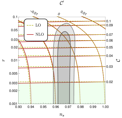
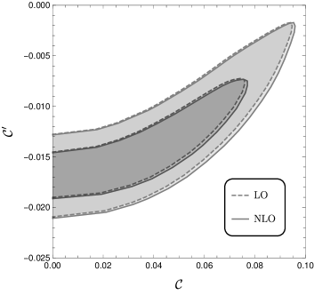
Figure 1: Relation between $(r,n_{s})$ and $(\mathcal{C},\mathcal{C}^{\prime})$ at LO and NLO, together with the bound (11) (shaded region) for $N=50$ and $\Delta\phi=M_{\rm Pl}$ (left); and experimental constrains on ($\mathcal{C},\mathcal{C}^{\prime})$ at LO and NLO from TT, TE, EE + lowE + lensing + BK15 + BAO data Akrami:2018odb (right).

In the next section we will particularize our study to inflationary potentials with $S$-duality symmetry. In particular, we will explore the relevance of the distance Swampland conjecture, which cannot be explored in a model independent way at any order.

III $\boldsymbol{S}$-duality strikes again

Dualities within gauge theories are striking as they relate a strongly coupled field theory to a weakly coupled one, and thereby they are handy for evaluating a theory at strong coupling, where perturbation theory breaks down, by translating it into its dual description with a weak coupling constant; ergo, dualities point to a single quantum system which has two classical limits. The $U(1)$ gauge theory on $\mathbb{R}^{4}$ is known to possess an electric-magnetic duality symmetry that inverts the coupling constant and extends to an action of $SL(2,\mathbb{Z})$ Montonen:1977sn . There are also many examples of $S$-duality in String Theory Font:1990gx ; Sen:1994fa . In this section we examine potentials which are invariant under the $S$ duality constraint and confront them with experiment. Herein we do not attempt a full association with a particular string vacuum, but simply regard the self-dual constraint as a relic of string physics in inflationary cosmology. We adopt a phenomenological approach to expand the inflationary potential in terms of a generic form satisfying the $S$-duality constraint and then the determination of the expansion coefficients is data driven.

For a real scalar field $\phi$, the $S$-duality symmetry is $\phi\to-\phi$ (or alternatively $g\rightarrow 1/g$, with $g\sim e^{\phi/M_{\rm Pl}}$). In case there is an imaginary part, i.e. an axion, then the $S$-duality group is extended to the modular group $SL(2,\mathbb{Z})$. The $S$-duality constraint forces a particular functional form on the inflationary potential: $V(\phi)=f[\cosh(\kappa\phi/M_{\rm Pl})]$, where $\kappa$ is a constant Anchordoqui:2014uua .

A compelling property of inflationary potentials featuring $S$-duality symmetry is that they resolve the “unlikeliness problem”, which is typical of plateau-like potentials, e.g.,

$$V_{1}(\phi)=\frac{V_{0}^{(1)}}{M_{\rm Pl}^{4}}\left(\phi^{2}-\phi_{0}^{2}\right)^{2},$$ (21)

where $V_{0}$ and $\phi_{0}$ are free parameters Ijjas:2013vea . Note that the plateau region satisfies $\phi\ll\phi_{0}$ terminating at the local minimum, and for large values of $\phi$ the potential grows as a power-law $\sim V_{0}(\phi/M_{\rm Pl})^{4}$. This means that we have two paths to reach the minimum of the potential: by slow-roll along the plateau or by slow-roll from the power-law side of the minimum. The problem appears because the path from the power-law side requires less fine tuning of parameters, has inflation occurring over a much wider range of $\phi$, and produces exponentially more inflation, but still CMB data prefer the unlikely path along the plateau.

The simplest $S$ self-dual form,

$$V_{2}(\phi)=V_{0}^{(2)}\ {\rm sech}\left(\frac{\kappa\phi}{M_{\rm Pl}}\right),$$ (22)

solves the unlikeliness problem because it has no power-law wall. Moreover, it is easily seen that for (21) and (22) the slow-roll parameters ${\epsilon}$ and $\eta$ are of the scale $(\phi_{0}/M_{\rm Pl})^{2}\sim\kappa^{-1}$ and thus have similar inflationary growths; see Fig. 2. However, for (21) the slow-roll parameters ${\epsilon}$ and $\eta$ grow fast near the end of inflation ($\phi\sim\phi_{0}$), but for the $S$ self-dual form ${\epsilon}$ and $\eta$ remain small because the potential has no local minimum. Thereby, $\phi$ cannot exit the inflationary period.

Figure 2: Potential and slow-roll functions for the potentials defined by (21) (solid line), and (22) with $\kappa=2$ (dotted), $\kappa=5$ (dashed) and $\kappa=10$ (dot-dashed).

To describe $S$-dual potentials for which inflation ends we adopt a polynomial expression in the sech function. Without loss of generality, we can write it as

$$V(\phi)=V_{0}\sum_{n=0}^{N}a_{n}\ \mathrm{sech}^{n}\left(\frac{\kappa\phi}{M_{\rm Pl}}\right)\,,$$ (23)

under the condition that $\sum_{i}a_{i}=1$, to ensure that $V_{0}=V(0)$. Here, the normalization constant $V_{0}$ and the expansion coefficients $a_{n}$ are determined empirically by matching experimental constraints. To determine the coefficients $a_{n}$ we demand:

• $N(\phi_{*}\to\phi_{e})\simeq 60$, with $\phi_{*}$ the field value when the $k_{*}$ scale crosses the horizon, $k_{*}=aH$;

• the NLO expression of $r$ given in (18) to satisfy the 95% CL upper limit, i.e. $r<0.069$ Akrami:2018odb ;

• the NLO expression of the scalar spectral index $n_{s}$ given in (14) to match the upper end of the measured $1\sigma$ value, $n_{s}\simeq 0.9698$ Akrami:2018odb .

The phenomenological expression in (22) could develop a minimum to support dissipative oscillations at the cessation of the slow roll and reheating, and resolves the unlikeliness problem. In order to analyze the model, it is convenient to define $y=\mathrm{sech}(\kappa\phi/M_{\rm Pl})$ and $V(\phi)=V_{0}f(y)$, with

$$f(y)=\sum_{n=0}^{N}a_{n}y^{n}.$$ (24)

Without conflicting with $S$-duality, we restrict ourselves here to $\phi>0$ to guarantee a bijection between $y$ and $\phi$. Note that $y\in[0,1]$ as $\phi\in[0,\infty)$. It is then easy to see that

$$V_{\phi}=-V_{0}\frac{\kappa}{M_{\rm Pl}}y\sqrt{1-y^{2}}f^{\prime}(y),$$ (25a)

$$V_{\phi\phi}=V_{0}\left(\frac{\kappa}{M_{\rm Pl}}\right)^{2}\left[\vphantom{\sum}y^{2}(1-y^{2})f^{\prime\prime}(y)+y(1-2y^{2})f^{\prime}(y)\right],$$ (25b)

and

$$V_{\phi\phi\phi}=V_{0}\left(\frac{\kappa}{M_{\rm Pl}}\right)^{3}y\sqrt{1-y^{2}}\left[\vphantom{\sum}-y^{2}(1-y^{2})f^{\prime\prime\prime}(y)-3y(1-2y^{2})f^{\prime\prime}(y)-(1-6y^{2})f^{\prime}(y)\right]$$ (25c)

which allow to obtain analytical expressions for $\epsilon$, $\eta$ and $\xi$.

Non-trivial potentials occur for $N\geq 2$. Here, we study the polynomial form in (22) at lowest order, i.e. $f(y)=a_{0}+a_{1}y+a_{2}y^{2}$. From the initially four model parameters $(V_{0},a_{1},a_{2},a_{3})$ the normalization condition $V(0)=V_{0}$ (or $f(1)=1)$ allows to remove one of them. The potential has a minimum, at which we can impose $V=0$, removing another constant. It is easily seen that in this case $f$ can be rewritten as

$$f(y)=\left(\frac{y-\beta}{1-\beta}\right)^{2},$$ (26)

where $\beta\in(0,1)$ is the position of the minimum. This corresponds to a potential

$$V(\phi)=V_{0}\left[\frac{\mathrm{sech}\left(\kappa\frac{\phi}{M_{\rm Pl}}\right)-\mathrm{sech}\left(\kappa\frac{\phi_{0}}{M_{\rm Pl}}\right)}{1-\mathrm{sech}\left(\kappa\frac{\phi_{0}}{M_{\rm Pl}}\right)}\right]^{2},$$ (27)

where $\beta=\mathrm{sech}\left(\kappa\phi_{0}/M_{\rm Pl}\right)$. A point worth noting at this juncture is that the the expansion of (23) is not hierarchical, i.e., the coefficients $a_{n}$ should not necessarily become smaller and smaller with larger $n$. Our choice is based on the complexity of the model, in which larger $N$ potentials would contain more free parameters and, under some conditions, more maxima/minima. Note that an identification of (24) with (26) allows one to see that $a_{1}/a_{0}=-2/\beta$ and $a_{2}/a_{1}=-1/2\beta$ and the hierarchy, if existing, is contingent on the position of the minimum of the field $\phi_{0}$ and on $\kappa$.

In Fig. 3 we show a comparison between the model described by (27) and the one introduced in (21). It is important to note that for small $\kappa$, both potentials become similar. Indeed, up to $\mathcal{O}(\kappa^{3})$ terms,

$$V(\phi)\approx\frac{V_{0}}{V_{0}^{(1)}}\left[\left(\frac{M_{\rm Pl}}{\phi_{0}}\right)^{4}-\frac{5}{6}\frac{\kappa^{2}M_{\rm Pl}^{2}}{\phi_{0}^{2}}\frac{\phi^{2}}{\phi_{0}^{2}}\right]V_{1}(\phi).$$ (28)

The zeroth order difference may be absorbed in the normalization of the potentials, so the potentials can be made almost identical for

$$\phi\lesssim\sqrt{\frac{6}{5}}\frac{M_{\rm Pl}}{\kappa}.$$ (29)

Then, only a relatively large $\kappa$ would produce substantial differences between both models if we want to avoid using highly trans-Planckian fields. For larger fields, the differences are more obvious, as $V_{1}$ grows indefinitely while

$$\lim_{\phi\to\infty}V(\phi)=\frac{V_{0}}{4}{\rm csch^{4}\,}\left(\frac{\kappa\phi_{0}}{2M_{\rm Pl}}\right).$$ (30)

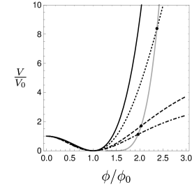
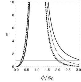
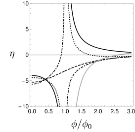
Figure 3: Potential and slow-roll functions for the potentials defined by (21) (solid line), and (27) with $\kappa=1/2$ (dotted), $\kappa=\ln(1+\sqrt{2})$ (dashed) and $\kappa=1$ (dot-dashed). The gray lines end of inflation ($\epsilon=1$).

The slow roll parameters can be now obtained from (25c) and (26), and are given by

$$\epsilon=\frac{2\kappa^{2}y^{2}(1-y^{2})}{(y-\beta)^{2}},$$ (31a)

$$\eta=\frac{2\kappa^{2}y\left(1-2y^{2}\right)}{y-\beta}$$ (31b)

and

$$\xi=\frac{4\kappa^{4}y^{2}\left(y^{2}-1\right)\left(\beta+2y\left(6y^{2}-3\beta y-2\right)\right)}{(y-\beta)^{3}};$$ (31c)

these can be easily combined with (14) and (18) to explore the parameter space in terms of $n_{s}$, $r$ and $N$. The first step in that direction requires to find out the condition(s) for slow roll to end. The potential under consideration allows for two types of slow roll inflation: (i) one in which $\phi$ rolls down the potential towards a minimum at larger values, and (ii) one in which a large field rolls down the potential towards smaller values. The condition $\epsilon=1$ may be rewritten as the quartic polynomial equation

$$y^{4}+\frac{1-2\kappa^{2}}{2\kappa^{2}}y^{2}-\frac{\beta}{\kappa^{2}}y+\frac{\beta^{2}}{2\kappa^{2}}=0,$$ (32)

which has, in principle, four complex roots, which may be obtained following Ferrari’s method Tignol:2001 . For the polynomial $y^{4}+qy^{2}+ry+s$, the roots are found to be

$$y=\sigma_{1}\sqrt{\frac{u}{2}}+\sigma_{2}\sqrt{-\frac{u}{2}-\frac{q}{2}-\sigma_{1}\frac{r}{2\sqrt{2u}}},$$ (33)

where $\sigma_{1}$ and $\sigma_{2}$ are two independent signs that generate the four solutions, and $u$ is a solution to the cubic equation $u^{3}+qu^{2}+(q^{2}/4-s)u-r^{2}/8=0$. This can be reduced by a change of variables $u=v-q/3$ to a depressed cubic equation $v^{3}-(s+q^{2}/12)v-(2q^{3}+27r^{2}-72qs)/216=0$. Such equation, generally $v^{3}+av+b=0$, has a solution given by Cardano’s formula $v=\sqrt[3]{\mathcal{A}_{+}}+\sqrt[3]{\mathcal{A}_{-}}$, with $\mathcal{A}_{\pm}=-b/2\pm\sqrt{\Delta}$ and $\Delta=(a/3)^{3}+(b/2)^{2}$ which, reverting the changes of variables, is

$$\Delta=-\frac{\beta^{2}}{2^{8}3^{3}\kappa^{8}}\left[32\kappa^{2}\beta^{4}+(1-8\kappa^{2}(5+4\kappa^{2})\beta^{2}-(1-2\kappa^{2})^{3}\right].$$ (34)

It is clear that the nature of the solutions depends on the sign of $\Delta$, which is unconstrained. The lines $\Delta=0$, which separate both regions, may be solved explicitly for $\beta$. Out of the four possible solutions, only

$$\beta_{0}(\kappa)=\frac{1}{8}\sqrt{-\frac{\left(16\kappa^{2}+1\right)^{3/2}}{\kappa^{2}}+32\kappa^{2}-\frac{1}{\kappa^{2}}+40}$$ (35)

is in the $\beta\in[0,1]$ and $\kappa>0$ region. The previous equation determines a limit in the $\kappa>1/\sqrt{2}$ region, value below which $\beta_{0}$ becomes complex. Moreover, $\kappa=\frac{1}{2}\sqrt{11+5\sqrt{5}}$ marks the point at which $\beta=1$. For $\beta>\beta_{0}(\kappa)$, $\Delta>0$. Then $\kappa<1/\sqrt{2}\Rightarrow\Delta>0$ and $\kappa>\frac{1}{2}\sqrt{11+5\sqrt{5}}\Rightarrow\Delta<0$. Conversely, $\Delta<0\Rightarrow\kappa>1/\sqrt{2}$ and $\Delta>0\Rightarrow\kappa<\frac{1}{2}\sqrt{11+5\sqrt{5}}$. For $1/\sqrt{2}<\kappa<\frac{1}{2}\sqrt{11+5\sqrt{5}}$ the curve $\beta_{0}(\kappa)$ separates both regions.

$\Delta>0$ —

In this case, $\mathcal{A}_{\pm}$ is real, and $u$ may be written directly as $u=\sqrt[3]{\mathcal{A}_{+}}+\sqrt[3]{\mathcal{A}_{-}}-q/3$. It it possible to see that $\mathcal{A}_{\pm}>0$ over the region where $\Delta>0$. Moreover, even if $q>0$ somewhere, $u>0$ everywhere. If $\sigma_{1}=+1$, $y$ is real and $\sigma_{2}$ generate both solutions. The case $\sigma_{1}=-1$ corresponds to complex solutions in all range where $\Delta>0$. Then, the two solutions of interest here are given by

$$y_{\pm}=\sqrt{\frac{u}{2}}\pm\sqrt{-\frac{u}{2}-\frac{q}{2}-\frac{r}{2\sqrt{2u}}}$$ (36a)

and

$$u=\left(-\frac{b}{2}+\sqrt{\left(\frac{b}{2}\right)^{2}+\left(\frac{a}{3}\right)^{3}}\right)^{\frac{1}{3}}+\left(-\frac{b}{2}-\sqrt{\left(\frac{b}{2}\right)^{2}+\left(\frac{a}{3}\right)^{3}}\right)^{\frac{1}{3}}-\frac{q}{3}.$$ (36b)

$\Delta<0$ —

In this case, the solution to the cubic equation contains complex terms, and it becomes convenient to define $\mathcal{A}_{\pm}=\mathcal{A}\exp(\pm i\theta)$, where $\mathcal{A}\equiv|\mathcal{A}_{\pm}|=\sqrt{b^{2}/4-\Delta}=\sqrt{-(a/3)^{3}}$ and $\theta=2\arctan[\sqrt{-\Delta}/(\mathcal{A}-b/2)]$, which allows to write $v=2\mathcal{A}^{\frac{1}{3}}\cos(\theta/3)$ and see that it is explicitly real. Moreover, as $\theta$ ranges in $[0,\pi]$, $\cos(\theta/3)$ is not negative. This, together with the fact that $q<0$ if $\kappa>1/\sqrt{2}$ makes $u$ positive as well. In this region, though, both values of $\sigma_{1}$ generate real solutions. It is clear that $\sigma_{1}=\sigma_{2}=-1$ would yield a negative solution, irrelevant in this case. Further investigation reveals that the other solution with $\sigma_{1}=-1$ yields negative solutions as well. The other solutions are always contained in $[0,1]$. Then, the solutions in this case are the same $y_{\pm}$ defined in (36a) where now $u$ is better expressed involving real numbers only as

$$u=2\sqrt{-\frac{a}{3}}\cos\left[\frac{2}{3}\arctan\left(\frac{\sqrt{-(b/2)^{2}-(a/3)^{3}}}{\sqrt{-(a/3)^{3}}-b/2}\right)\right]-\frac{q}{3}.$$ (37)

The parameters $a$, $b$ and $q$ used in all solutions above are

$$a=-\frac{\beta^{2}}{2\kappa^{2}}-\frac{\left(1-2\kappa^{2}\right)^{2}}{48\kappa^{4}},$$ (38a)

$$b=\frac{\beta^{2}\left(1-2\kappa^{2}\right)}{12\kappa^{4}}-\frac{\beta^{2}}{8\kappa^{4}}-\frac{\left(1-2\kappa^{2}\right)^{3}}{864\kappa^{6}},$$ (38b)

and

$$q=\frac{1-2\kappa^{2}}{2\kappa^{2}}.$$ (38c)

The solutions $y_{\pm}$ to the end of inflation equation $\epsilon=1$ are shown in Fig. 4. We recall here that $y_{-}$ corresponds to a solution for smaller $y$ (larger $\phi$), and $y_{+}$ to larger $y$ (smaller $\phi$). We define $y_{\pm}=\mathrm{sech}(\kappa\phi_{\pm}/M_{\rm Pl})$.

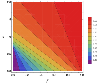
(a)  Solution $y_{+}$ from (36a).

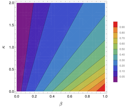
(b)  Solution $y_{-}$ from (36a).

Figure 4: Exploration of the solutions $y_{\pm}$ to the end of inflation condition $\epsilon=1$.

We can now proceed with our analysis noting that, besides the values of $\beta$ and $\kappa$, which determine the end of inflation, there is still freedom in choosing the value of the field at the scale that corresponds to the experimental values. We call this $\phi_{*\pm}$ and define $\delta_{\pm}=\pm(\phi_{\pm}-\phi_{*\pm})/M_{\rm Pl}$. We recall that the distance Swampland conjecture demands that $\delta_{\pm}\lesssim\mathcal{O}(1)$. In terms of our model, when we are considering large fields (minus signs above), the value of $\phi_{*-}$ is unbounded and $\delta_{-}$ could take any positive value. Nevertheless, for small fields (plus signs above) $\delta_{+}$ is constrained so that $\phi_{*+}>0$, which means $\delta_{+}<\phi_{+}/M_{\rm Pl}$. All in all, the corresponding values for $y$ are

$$y_{*\pm}=\mathrm{sech}\left(\vphantom{\sum}\mathrm{arcsech}\,y_{\pm}\mp\kappa\delta_{\pm}\right)$$ (39)

where $\delta_{+}<\kappa^{-1}\mathrm{arcsech}\,y_{+}$. A choice of values $(\beta,\kappa,\delta)$ and a branch (large or small $\phi)$ specifies the model completely. In specifically, the values for $y_{\pm}$ and $y_{*\pm}$ described above can be used to calculate the slow roll functions at $y_{*\pm}$ and, subsequently, the values of $n_{s}$ and $r$; and the number of $e$-folds between $y_{*\pm}$ and $y_{\pm}$. Finally, we also study the number of inflation $e$-folds produced corresponding to the different parameters, which can be obtained from (9) to be

$$N=\frac{2\beta\left(\frac{1}{y_{*\pm}}-\frac{1}{y_{\pm}}\right)+(1-\beta)\ln\left(\frac{1-y_{\pm}}{1-y_{*\pm}}\right)+(1+\beta)\ln\left(\frac{1+y_{\pm}}{1+y_{*\pm}}\right)-2\ln\left(\frac{y_{\pm}}{y_{*\pm}}\right)}{4\kappa^{2}}.$$ (40)

Figure 5: Exploration of the $(\kappa,\delta)$ parameter space for a fixed $\beta=0.5$. The dashed curves in black (white) are for constant $\delta$ ($\kappa$). The solid lines contain the relations between $(\mathcal{C},\mathcal{C}^{\prime})$ and $(r_{s},r)$ for the model (i.e. for the actual $\xi$ obtained from (31c)). The experimental bounds are as in Fig. 1.

Our results for the large field solution (corresponding to $y_{-}$) with $\beta=0.5$ are encapsulated in Fig. 5. The results show a mixed degree of compatibility between the Swampland conjectures and experimental data for the $S$-dual potential. The model itself can easily accommodate the experimental constrains for some region of the parameter space (namely $\kappa\gtrsim 1$ and $\delta\lesssim 1$), as $n_{s}$, $r$, and $50\lesssim N\lesssim 60$ are all reproducible. We can further study the compatibility between the de Sitter conjecture, the distance conjecture, and the experimental results. It is clearly visible how the bound on $\mathcal{C}$ from the de Sitter conjecture and the requirement on $\Delta\phi$ from the distance conjecture are in tension, as values of $\mathcal{C}\sim\mathcal{O}(1)$ even for the $95\%\,\mathrm{CL}$ lower limit on $n_{s}$ at $0.959$ require $\delta\gg 1$. On the other hand, the de Sitter bound on $\mathcal{C}^{\prime}$ and the distance conjecture set bounds that get softer in the same direction of decreasing $r$. In this case, $\mathcal{C}^{\prime}$ is constrained by the data at the $95\%\,\mathrm{CL}$ lower limit on $n_{s}$ to $\mathcal{C}^{\prime}\gtrsim-0.02$. Despite this experimental constraint being much stronger than the $\mathcal{C}\lesssim 0.09$, there is no strong incompatibility with the distance conjecture.

As a final remark, we study the strength of Lyth’s bound (11) on the current model, i.e. to which extent the model saturates such bound. In Fig. 6 we show the value of $N\mathcal{C}/\delta$ as obtained from (40) as a function of $\kappa$ and $\delta$, which is bound above by $1$ by means of Lyth’s bound. It is visible that only for small values of $\delta$ Lyth’s bound is saturated.

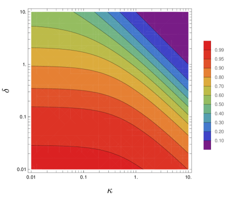
Figure 6: Value of $N\mathcal{C}/\delta$, bound to be lower than one by (11), as a function of $(\kappa,\delta)$ for $\beta=0.5$.

IV Ambiguity in slow-roll parameter definitions and impact on the Swampland conjectures

It is common in the literature to observe two different definitions of the slow-roll parameters, one defined in terms of the Hubble parameter $H$, and other in terms of the potential $V$; we have used the latter in previous sections. We have seen that the slow-roll parameters of single field inflation defined by $V$ are in tension with the Swampland conjectures. An interesting question we explore in this section is whether these two choices of parameters differ in a significant way, so that the tension with the Swampland conjectures can be reduced.

Accelerated expansion occurs as long as $\ddot{a}>0$, and, since

$$\frac{\ddot{a}}{aH^{2}}=1+\frac{\dot{H}}{H^{2}},$$ (41)

that condition may be rewritten as $-\dot{H}/H^{2}<1$. The slow-roll limit means that $H$ is constant, as this is the only way to support exponential expansion with $a=\exp(Ht)$. The slow-roll regime may be considered as that in which $H$ changes slowly, which is what motivates the definition of the dimensionless slow roll parameter as

$$\epsilon_{H}=-\frac{\dot{H}}{H^{2}},$$ (42)

for which $\epsilon_{H}<1$ means accelerated expansion, $\epsilon\ll 1$ means slow-roll expansion, and $\epsilon_{H}=0$ means exponential expansion. Using the Friedmann equation

$$H^{2}=\frac{1}{3M_{\rm Pl}^{2}}\left(V+\frac{1}{2}\dot{\phi}^{2}\right)$$ (43)

and the equation of motion (3), this may be rewritten as

$$\epsilon_{H}=3\frac{\dot{\phi}^{2}/2}{V+\dot{\phi}^{2}/2}=2M_{\rm Pl}^{2}\left(\frac{H_{\phi}}{H}\right)^{2},$$ (44)

where we have made use of the relation $\dot{\phi}^{2}=-2M_{\rm Pl}^{2}\dot{H}$. In order to connect this to the $V$-parameters, we write

$$\frac{H_{\phi}}{H}=-\frac{3H\dot{\phi}}{6M_{\rm Pl}^{2}H^{2}}=\frac{V_{\phi}+\ddot{\phi}}{6M_{\rm Pl}^{2}H^{2}},$$ (45)

and

$$\epsilon_{H}=\frac{M_{\rm Pl}^{2}}{2}\left(\frac{V_{\phi}+\ddot{\phi}}{V+\dot{\phi}^{2}/2}\right)^{2}.$$ (46)

The slow-roll condition $\epsilon_{H}\ll 1$ directly implies that $V\gg\dot{\phi}^{2}/2$, in which case

$$\epsilon_{H}\approx\frac{M_{\rm Pl}^{2}}{2}\left(\frac{V_{\phi}+\ddot{\phi}}{V}\right)^{2}.$$ (47)

If one further imposes the condition that $|\ddot{\phi}|\ll|V_{\phi}|$, the approximation

$$\epsilon_{H}\approx\frac{M_{\rm Pl}^{2}}{2}\left(\frac{V_{\phi}}{V}\right)^{2}$$ (48)

is valid. This motivates the definition of the $V$-parameter as

$$\epsilon_{V}\equiv\frac{M_{\rm Pl}^{2}}{2}\left(\frac{V_{\phi}}{V}\right)^{2},$$ (49)

The question of whether $\epsilon_{H}$ and $\epsilon_{V}$ may be approximately equal depends on whether the two approximations used to derive (48) are simultaneously satisfied. A glance at (44) suggests that they may not always be, as in the limit $\dot{\phi}\to 0$, $\epsilon_{H}\to 0$ while $\epsilon_{V}$ may take any finite value. Moreover, one can rewrite the equation of motion as

$$(V_{\phi}+\ddot{\phi})^{2}=\frac{3}{M_{\rm Pl}^{2}}\dot{\phi}^{2}(V+\dot{\phi}^{2}/2)$$ (50)

to see that a condition on the smallness of $\dot{\phi}^{2}$ doesn’t guarantee the smallness of $\ddot{\phi}$ with respect to $V_{\phi}$ unless $V_{\phi}$ is itself small. We conclude that, in general, both conditions must be separately satisfied to guarantee the similarity between $\epsilon_{H}$ and $\epsilon_{V}$. A more comprehensive study of the differences between both parameters (as well as the second order ones, $\eta_{H}$ and $\eta_{V}$), can be found in Liddle:1994 . Here we highlight only the aspects relevant for our discussion.

Given a specific potential $V(\phi)$, one can obtain a solution $\phi(t)$ to the equation of motion, subject to the initial conditions $\phi(t_{0})=\phi_{0}$ and $\dot{\phi}(t_{0})=\dot{\phi}_{0}$. This makes the difference between $\epsilon_{V}$ and $\epsilon_{H}$ explicit, since at $t=t_{0}$ the former depends only on $\phi_{0}$ while the latter depends on both $\phi_{0}$ and $\dot{\phi}_{0}$. Therefore, the equality or similarity between $\epsilon_{V}$ and $\epsilon_{H}$ is a matter of a handpicked pair $(\phi_{0},\dot{\phi}_{0})$ that would guarantee both $\dot{\phi}^{2}/2\ll V$ and $|\ddot{\phi}|\ll V_{\phi}$.

This makes clear that the end of inflation condition $\epsilon_{H}=1$ would yield different results than $\epsilon_{V}=1$. While the latter condition is the most commonly used, and is simpler to evaluate due to its sole dependence on the shape of the potential, it is the former condition that must be satisfied exactly, since it depends on the full solution of the scalar field equation of motion.

A judicious choice of initial conditions on the field and its derivative at the time at which the scale $k_{*}$ crosses the horizon should be able to accommodate multiple values of $\mathcal{C}$ or $\mathcal{C}^{\prime}$, potentially reducing the tensions with the Swampland conjectures, while remaining in the $H$-dictated slow-roll regime. Nevertheless, keeping the de Sitter conjecture and the observed number of inflation $e$-folds under control is not guaranteed in this situation. A full study like the one presented in Sec. III, adding these initial conditions, should be considered if one aims to characterize the complete parameter space. Nevertheless, we leave that for future work, as the increase in computational complexity escapes the aim of this paper. Here, instead, we choose initial conditions that optimize the comparison between the $H$-parameters and the $V$-parameters, rather than the generality of the study.

To remove part of the ambiguity caused by the freedom of choice in the initial conditions, we consider $t_{*}$ (the time at which the scale $k_{*}$ crosses the horizon) as the starting point for the solution to the equation of motion. In order to reduce the number of quantities affected by the choice of parameters, we choose to leave the observable values of $n_{s}$ and $r$ unaffected. Since these values depend on $\epsilon$ and $\eta$ at $t_{*}$, fixing the initial conditions on $\phi$ such that $\epsilon_{H}(t_{*})=\epsilon_{V}(t_{*})$ allows to remove any effect of this choice on them. This is just an operational perspective that should allow us to compare the differences that $\epsilon_{H}$ and $\epsilon_{V}$ have only in regard to the other observable, $N$. This condition amounts to

$$\dot{\phi}^{2}(t_{*})=\frac{2V(\phi_{*})}{3/\epsilon_{V}(\phi_{*})-1},$$ (51)

which may be rewritten in terms of $y$ as

$$\dot{y}(t_{*})=\frac{\sqrt{{V_{0}}}}{M_{\rm Pl}}\frac{2\kappa^{2}{y_{0}}^{2}(\beta-y_{0})\left(1-{y_{0}}^{2}\right)}{(1-\beta)\sqrt{3({y_{0}}-\beta)^{2}-2\kappa^{2}{y_{0}}^{2}\left(1-{y_{0}}^{2}\right)}}.$$ (52)

In a similar manner as we proceeded before, we start by fixing the model parameters $(\beta,\kappa)$, and finding the end of inflation using the $\epsilon_{V}(y_{\mathrm{e},V})=1$ condition, and the value of $y_{*}$ via (39), using a given value of $\delta$, named here $\delta_{V}$. With both $y_{*}$ and $y_{\mathrm{e},V}$ we can find the value of $N_{V}$ using (40). To quantify the difference between the choice of $\epsilon_{V}$ and of $\epsilon_{H}$, we calculate the true end of inflation through the $\epsilon_{H}(y_{\mathrm{e},H})=1$ condition, which provides a true value for $\delta$, as $\delta_{H}=\kappa^{-1}(\mathrm{arcsech}\,y_{*}-\mathrm{arcsech}\,y_{\mathrm{e},H})$, and a true number of $e$-folds $N_{H}$ as

$$N_{H}=-\frac{1}{M_{\rm Pl}}\int_{\phi_{*}}^{\phi_{e}}\frac{d\phi}{\sqrt{2\epsilon_{H}}}=\frac{1}{\kappa}\int_{t_{*}}^{t_{\mathrm{e},H}}\frac{\dot{y}}{y\sqrt{1-y^{2}}\sqrt{2\epsilon_{H}}}dt,$$ (53)

where $t_{\mathrm{e},H}$ is the true time at which inflation ends.

In Fig. 7(a) we show the relation between $N_{V}$ and $\delta_{V}$, and $N_{H}$ and $\delta_{H}$. While a full analysis similar to that presented in Fig. 5 might be the only way to fully understand the relevance of the parameter set choice, here it is visible how the difference $\Delta N\equiv N_{H}-N_{V}$ grows both with $\kappa$ and $\delta$. We can see in Fig. 7(b) that for small values of $\kappa$, which are of more interest in the study of the de Sitter conjecture on $\mathcal{C}$, $\Delta N$ is small enough to make it irrelevant, and no significant difference would be expected in that front. Regarding $\mathcal{C}^{\prime}$, the $\mathcal{C}^{\prime}\gtrsim-0.02$ experimental bound may be accommodated a bit easier regarding the number of $e$-folds, as in that region the constraint $\epsilon_{V}=1$ is underestimating the number of $e$-folds by a few percent points of its true value.

Nevertheless, despite the minor changes introduced in relation to the Swampland conjectures, Fig. 7(b) makes clear that the $\epsilon_{V}=1$ condition might end inflation too early, producing considerable underestimations of the actual number of $e$-folds.

We want to remind the reader that these results are obtained for $\beta=0.5$, as was the case with the results presented in and after Fig. 5. It must also be clarified that the information presented in Fig. 7(a) and Fig. 7(b) is not in contradiction, unlike it may seem. Fig. 7(a) presents the curves $N_{H}(\delta_{H})$ and $N_{V}(\delta_{V})$, so the horizontal axis is not the same variable, and makes it seem that for a single $\delta$, the $V$-based condition overestimates the number of $e$-folds. Nevertheless, in Fig. 7(b) we show the curves evaluated at the same value of $\delta$. This is therefore comparing the two parameter choices for a fixed value of the field excursion $\Delta\phi$. Under this circumstance, it is clearly seen that the $V$-based conditions produce an underestimation of the number of inflation $e$-folds with respect to the $H$-based ones.

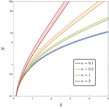
(a)  $N$ as a function of $\delta$ for the $\epsilon_{H}=1$ (solid) and $\epsilon_{V}=1$ (dashed) conditions.

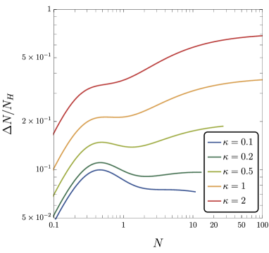
(b)  Underestimation of $N$ with $\epsilon_{V}=1$ relative to $\epsilon_{H}=1$.

Figure 7: Comparison of the two end of inflation conditions, $\epsilon_{H}=1$ and $\epsilon_{V}=1$, regarding their effect on the number of inflation $e$-folds and the parameter $\delta$.

V Conclusions

We have analyzed the most general form of single-field $S$-dual inflationary potentials at NLO in slow-roll parameters within the context of the Swampland program and confronted model predictions with experiment. We have found that to accommodate the 95% CL limit on $r<0.068$ form BICEP2/Keck Array + Planck + BAO data Ade:2018gkx ; Akrami:2018odb we require $c\sim{\cal O}(10^{-1})$. This requirement is in tension with the de Sitter conjecture. However, in the spirit of Dias:2018ngv , we can adopt a conservative approach and regard the de Sitter conjecture as a parametric constraint where the inequality (1) holds, but the number $c$ may not be strictly ${\cal O}(1)$. Indeed, it is easy to established a mass hierarchy between the lightest moduli field and and inflaton to accommodate $c\sim{\cal O}(10^{-1})$ Dias:2018ngv . From this viewpoint, constraints on inflation can then be used to constrain $c$. Still, as we have shown in Fig. 5 to accommodate $c\sim{\cal O}(10^{-1})$ a $\delta\sim{\cal O}(10)$ would be required. To be able to match such a large value of $\delta$ we must explore the subtleties of the distance conjecture, which asserts that for any infinite field distance limit, an infinite tower of states becomes exponentially light, and therefore EFTs are only valid for finite scalar field variations Ooguri:2006in ; Klaewer:2016kiy ; Ooguri:2018wrx ; Grimm:2018ohb ; Heidenreich:2018kpg . This in turn implies a quantum gravity cutoff associated to the infinite tower of states, decreasing exponentially in terms of the proper field distance, $\Lambda_{\rm QG}=\Lambda_{\rm self}\ e^{-\lambda\,\Delta\phi}$, where $\Lambda_{\rm QG}$ is the quantum gravity cutoff, $\Lambda_{\rm self}$ is the cutoff of the EFT, and $\lambda$ is argued to be of order unity in Planck units (see, however, Andriot:2020lea ; Gendler:2020dfp ). Now, since $\Lambda_{\rm self}\leq M_{\rm Pl}$ we have $\Delta\phi\leq\lambda^{-1}\ln(M_{\rm Pl}/\Lambda_{\rm self})$, which indicates that the maximum field variation actually depends on the cutoff of the EFT vanBeest:2021lhn . We know that for EFT to describe inflation, its cutoff must be above the Hubble scale, i.e. $\Lambda_{\rm self}>H$. If we adopt the conservative bound $\Lambda_{\rm self}\sim H$, then $\Delta\phi\lesssim 10~{}M_{\rm Pl}$ Scalisi:2018eaz . Needless to say, it should be stressed that the EFT will likely break down (or at least get sensitive to the infinite tower) before the mass of the first state becomes of order Hubble, so the constraints might be stronger than those derived from the assumption $\Lambda_{\rm self}\sim H$. Next-generation CMB satellites searching for primordial B-modes (e.g. PIXIE Khatri:2013dha , CORE Finelli:2016cyd , and LiteBIRD Hazumi:2019lys ) will reach a 95%CL sensitivity of $r<0.002$. This will allow discrimination between small-field $\Delta\phi<M_{\rm Pl}$ and large-field $\Delta\phi>M_{\rm Pl}$ inflationary models, and will provide a final verdict for the ideas presented and discussed in this paper.

As a final remark, it would be interesting to study the full parameter space using the $H$-parameters introduced in Sec. IV rather than the $V$-parameters. As stated there, the increase in the number free parameters would make it more feasible to reduce the tension with the Swampland conjectures. An analysis like the one presented here in which the $H$-parameters are used in full is left for future work.

- (1) A. H. Guth, The inflationary universe: A possible solution to the horizon and flatness problems, Phys. Rev. D 23, 347-356 (1981) doi:10.1103/PhysRevD.23.347
- (2) A. D. Linde, A new inflationary universe scenario: A possible solution of the horizon, flatness, homogeneity, isotropy and primordial monopole problems, Phys. Lett. B 108, 389-393 (1982) doi:10.1016/0370-2693(82)91219-9
- (3) A. Albrecht and P. J. Steinhardt, Cosmology for grand unified theories with radiatively induced symmetry breaking, Phys. Rev. Lett. 48, 1220-1223 (1982)
- (4) V. F. Mukhanov and G. V. Chibisov, Quantum fluctuations and a nonsingular universe, JETP Lett. 33, 532-535 (1981)
- (5) S. W. Hawking, The development of irregularities in a single bubble inflationary universe, Phys. Lett. B 115, 295 (1982) doi:10.1016/0370-2693(82)90373-2
- (6) A. H. Guth and S. Y. Pi, Fluctuations in the new inflationary universe, Phys. Rev. Lett. 49, 1110-1113 (1982) doi:10.1103/PhysRevLett.49.1110
- (7) A. A. Starobinsky, Dynamics of phase transition in the new inflationary universe scenario and generation of perturbations, Phys. Lett. B 117, 175-178 (1982) doi:10.1016/0370-2693(82)90541-X
- (8) J. M. Bardeen, P. J. Steinhardt and M. S. Turner, Spontaneous creation of almost scale-free density perturbations in an inflationary universe, Phys. Rev. D 28, 679 (1983) doi:10.1103/PhysRevD.28.679
- (9) D. N. Spergel et al. [WMAP Collaboration], First year Wilkinson Microwave Anisotropy Probe (WMAP) observations: Determination of cosmological parameters, Astrophys. J. Suppl. 148, 175-194 (2003) doi:10.1086/377226 [arXiv:astro-ph/0302209 [astro-ph]].
- (10) E. Komatsu et al. [WMAP Collaboration], Seven-year Wilkinson Microwave Anisotropy Probe (WMAP) observations: Cosmological interpretation, Astrophys. J. Suppl. 192, 18 (2011) doi:10.1088/0067-0049/192/2/18 [arXiv:1001.4538 [astro-ph.CO]].
- (11) Y. Akrami et al. [Planck Collaboration], Planck 2018 results X: Constraints on inflation, Astron. Astrophys. 641, A10 (2020) doi:10.1051/0004-6361/201833887 [arXiv:1807.06211 [astro-ph.CO]].
- (12) P. A. R. Ade et al. [BICEP2 and Keck Array Collaboration], Constraints on primordial gravitational waves using Planck, WMAP, and new BICEP2/Keck observations through the 2015 season, Phys. Rev. Lett. 121, 221301 (2018) doi:10.1103/PhysRevLett.121.221301 [arXiv:1810.05216 [astro-ph.CO]].
- (13) P. A. R. Ade et al. [Planck Collaboration], Planck 2015 results. XX. Constraints on inflation, Astron. Astrophys. 594, A20 (2016) doi:10.1051/0004-6361/201525898 [arXiv:1502.02114 [astro-ph.CO]].
- (14) C. Vafa, The String landscape and the swampland, hep-th/0509212.
- (15) C. Montonen and D. I. Olive, Magnetic monopoles as gauge particles?, Phys. Lett. B 72, 117 (1977). doi:10.1016/0370-2693(77)90076-4
- (16) A. Font, L. E. Ibanez, D. Lüst and F. Quevedo, Strong - weak coupling duality and nonperturbative effects in string theory, Phys. Lett. B 249, 35 (1990). doi:10.1016/0370-2693(90)90523-9
- (17) A. Sen, Strong - weak coupling duality in four-dimensional string theory, Int. J. Mod. Phys. A 9, 3707 (1994) doi:10.1142/S0217751X94001497 [hep-th/9402002].
- (18) T. D. Brennan, F. Carta and C. Vafa, The String Landscape, the Swampland, and the missing corner, PoS TASI 2017, 015 (2017) doi:10.22323/1.305.0015 [arXiv:1711.00864 [hep-th]].
- (19) E. Palti, The Swampland: introduction and review,” Fortsch. Phys. 67, no. 6, 1900037 (2019) doi:10.1002/prop.201900037 [arXiv:1903.06239 [hep-th]].
- (20) N. Arkani-Hamed, L. Motl, A. Nicolis and C. Vafa, The String landscape, black holes and gravity as the weakest force, JHEP 0706, 060 (2007) doi:10.1088/1126-6708/2007/06/060 [hep-th/0601001].
- (21) H. Ooguri and C. Vafa, On the geometry of the String Landscape and the Swampland, Nucl. Phys. B 766, 21 (2007) doi:10.1016/j.nuclphysb.2006.10.033 [hep-th/0605264].
- (22) D. Klaewer and E. Palti, Super-Planckian spatial field variations and quantum gravity, JHEP 1701, 088 (2017) doi:10.1007/JHEP01(2017)088 [arXiv:1610.00010 [hep-th]].
- (23) H. Ooguri, E. Palti, G. Shiu and C. Vafa, Distance and de Sitter conjectures on the Swampland, Phys. Lett. B 788, 180 (2019) doi:10.1016/j.physletb.2018.11.018 [arXiv:1810.05506 [hep-th]].
- (24) T. W. Grimm, E. Palti and I. Valenzuela, Infinite distances in field space and massless towers of states, JHEP 1808, 143 (2018) doi:10.1007/JHEP08(2018)143 [arXiv:1802.08264 [hep-th]].
- (25) B. Heidenreich, M. Reece and T. Rudelius, Emergence of weak coupling at large distance in quantum gravity, Phys. Rev. Lett. 121, no. 5, 051601 (2018) doi:10.1103/PhysRevLett.121.051601 [arXiv:1802.08698 [hep-th]].
- (26) H. Ooguri and C. Vafa, Non-supersymmetric AdS and the Swampland, Adv. Theor. Math. Phys. 21, 1787 (2017) doi:10.4310/ATMP.2017.v21.n7.a8 [arXiv:1610.01533 [hep-th]].
- (27) E. Palti, The weak gravity conjecture and scalar fields, JHEP 1708, 034 (2017) doi:10.1007/JHEP08(2017)034 [arXiv:1705.04328 [hep-th]].
- (28) G. Obied, H. Ooguri, L. Spodyneiko and C. Vafa, de Sitter Space and the Swampland, arXiv:1806.08362 [hep-th].
- (29) D. Andriot, On the de Sitter swampland criterion, Phys. Lett. B 785, 570 (2018) doi:10.1016/j.physletb.2018.09.022 [arXiv:1806.10999 [hep-th]].
- (30) A. Kehagias and A. Riotto, A note on Inflation and the Swampland, Fortsch. Phys. 66, no.10, 1800052 (2018) doi:10.1002/prop.201800052 [arXiv:1807.05445 [hep-th]].
- (31) S. Cecotti and C. Vafa, Theta-problem and the String Swampland,” arXiv:1808.03483 [hep-th].
- (32) D. Klaewer, D. Lüst and E. Palti, A spin-2 conjecture on the Swampland, Fortsch. Phys. 67, no. 1-2, 1800102 (2019) doi:10.1002/prop.201800102 [arXiv:1811.07908 [hep-th]].
- (33) J. J. Heckman and C. Vafa, Fine tuning, sequestering, and the Swampland, doi:10.1016/j.physletb.2019.135004 arXiv:1905.06342 [hep-th].
- (34) D. Lüst, E. Palti and C. Vafa, AdS and the Swampland, doi:10.1016/j.physletb.2019.134867 arXiv:1906.05225 [hep-th].
- (35) A. Bedroya and C. Vafa, Trans-Planckian censorship and the Swampland, arXiv:1909.11063 [hep-th].
- (36) A. Kehagias, D. Lüst and S. Lüst, Swampland, gradient flow and infinite distance, arXiv:1910.00453 [hep-th].
- (37) R. Blumenhagen, M. Brinkmann and A. Makridou, Quantum log-corrections to Swampland conjectures, arXiv:1910.10185 [hep-th].
- (38) D. Andriot, N. Cribiori and D. Erkinger, The web of swampland conjectures and the TCC bound, JHEP 07, 162 (2020) doi:10.1007/JHEP07(2020)162 [arXiv:2004.00030 [hep-th]].
- (39) N. Gendler and I. Valenzuela, Merging the weak gravity and distance conjectures using BPS extremal black holes, JHEP 01, 176 (2021) doi:10.1007/JHEP01(2021)176 [arXiv:2004.10768 [hep-th]].
- (40) Q. Bonnefoy, L. Ciambelli, D. Lüst and S. Lüst, The Swampland at large number of space-time dimensions, [arXiv:2011.06610 [hep-th]].
- (41) E. Perlmutter, L. Rastelli, C. Vafa and I. Valenzuela, A CFT distance conjecture, [arXiv:2011.10040 [hep-th]].
- (42) M. Lüben, D. Lüst and A. R. Metidieri, The black hole entropy distance conjecture and black hole evaporation, Fortsch. Phys. 69, no.3, 2000130 (2021) doi:10.1002/prop.202000130 [arXiv:2011.12331 [hep-th]].
- (43) J. Calderón-Infante, A. M. Uranga and I. Valenzuela, The convex hull Swampland distance conjecture and bounds on non-geodesics, [arXiv:2012.00034 [hep-th]].
- (44) E. W. Kolb, A. J. Long and E. McDonough, Catastrophic production of slow gravitinos, [arXiv:2102.10113 [hep-th]].
- (45) D. H. Lyth, What would we learn by detecting a gravitational wave signal in the cosmic microwave background anisotropy?, Phys. Rev. Lett. 78, 1861-1863 (1997) doi:10.1103/PhysRevLett.78.1861 [arXiv:hep-ph/9606387 [hep-ph]].
- (46) P. Agrawal, G. Obied, P. J. Steinhardt and C. Vafa, On the cosmological implications of the String Swampland, Phys. Lett. B 784, 271-276 (2018) doi:10.1016/j.physletb.2018.07.040 [arXiv:1806.09718 [hep-th]].
- (47) A. Achúcarro and G. A. Palma, The string swampland constraints require multi-field inflation, JCAP 02, 041 (2019) doi:10.1088/1475-7516/2019/02/041 [arXiv:1807.04390 [hep-th]].
- (48) S. K. Garg and C. Krishnan, Bounds on slow roll and the de Sitter Swampland, JHEP 11, 075 (2019) doi:10.1007/JHEP11(2019)075 [arXiv:1807.05193 [hep-th]].
- (49) I. Ben-Dayan, Draining the Swampland, Phys. Rev. D 99, no.10, 101301 (2019) doi:10.1103/PhysRevD.99.101301 [arXiv:1808.01615 [hep-th]].
- (50) W. H. Kinney, S. Vagnozzi and L. Visinelli, The zoo plot meets the swampland: mutual (in)consistency of single-field inflation, string conjectures, and cosmological data, Class. Quant. Grav. 36, no.11, 117001 (2019) doi:10.1088/1361-6382/ab1d87 [arXiv:1808.06424 [astro-ph.CO]].
- (51) H. Fukuda, R. Saito, S. Shirai and M. Yamazaki, Phenomenological consequences of the refined swampland conjecture, Phys. Rev. D 99, no.8, 083520 (2019) doi:10.1103/PhysRevD.99.083520 [arXiv:1810.06532 [hep-th]].
- (52) S. K. Garg, C. Krishnan and M. Zaid Zaz, Bounds on slow roll at the boundary of the Landscape, JHEP 03, 029 (2019) doi:10.1007/JHEP03(2019)029 [arXiv:1810.09406 [hep-th]].
- (53) P. Agrawal and G. Obied, Dark energy and the refined de Sitter conjecture, JHEP 06, 103 (2019) doi:10.1007/JHEP06(2019)103 [arXiv:1811.00554 [hep-ph]].
- (54) C. I. Chiang, J. M. Leedom and H. Murayama, What does inflation say about dark energy given the swampland conjectures?, Phys. Rev. D 100, no.4, 043505 (2019) doi:10.1103/PhysRevD.100.043505 [arXiv:1811.01987 [hep-th]].
- (55) E. W. Kolb and S. L. Vadas, Relating spectral indices to tensor and scalar amplitudes in inflation, Phys. Rev. D 50, 2479-2487 (1994) doi:10.1103/PhysRevD.50.2479 [arXiv:astro-ph/9403001 [astro-ph]].
- (56) S. Dodelson, W. H. Kinney and E. W. Kolb, Cosmic microwave background measurements can discriminate among inflation models, Phys. Rev. D 56, 3207-3215 (1997) doi:10.1103/PhysRevD.56.3207 [arXiv:astro-ph/9702166 [astro-ph]].
- (57) J. E. Lidsey, A. R. Liddle, E. W. Kolb, E. J. Copeland, T. Barreiro and M. Abney, Reconstructing the inflation potential: An overview, Rev. Mod. Phys. 69, 373 (1997) doi:10.1103/RevModPhys.69.373 [astro-ph/9508078].
- (58) G. N. Remmen and S. M. Carroll, How many -folds should we expect from high-scale inflation?, Phys. Rev. D 90, no.6, 063517 (2014) doi:10.1103/PhysRevD.90.063517 [arXiv:1405.5538 [hep-th]].
- (59) S. M. Leach, A. R. Liddle, J. Martin and D. J. Schwarz, Cosmological parameter estimation and the inflationary cosmology, Phys. Rev. D 66, 023515 (2002) doi:10.1103/PhysRevD.66.023515 [arXiv:astro-ph/0202094 [astro-ph]].
- (60) L. A. Anchordoqui, V. Barger, H. Goldberg, X. Huang and D. Marfatia, -dual Inflation: BICEP2 data without unlikeliness, Phys. Lett. B 734, 134-136 (2014) doi:10.1016/j.physletb.2014.05.046 [arXiv:1403.4578 [hep-ph]].
- (61) A. Ijjas, P. J. Steinhardt and A. Loeb, Inflationary paradigm in trouble after Planck2013, Phys. Lett. B 723, 261 (2013) doi:10.1016/j.physletb.2013.05.023 [arXiv:1304.2785 [astro-ph.CO]].
- (62) J.-P. Tignol, Galois’ Theory of Algebraic Equations, World Scientific (2001) doi:10.1142/4628.
- (63) A. R. Liddle, P. Parsons and J. D. Barrow, Formalizing the slow-roll approximation in inflation, Phys. Rev. D 50, no.12, 7222 (1994) doi:10.1103/PhysRevD.50.7222 [arXiv:astro-ph/9408015].
- (64) M. Dias, J. Frazer, A. Retolaza and A. Westphal, Primordial gravitational waves and the swampland, Fortsch. Phys. 67, no.1-2, 2 (2019) doi:10.1002/prop.201800063 [arXiv:1807.06579 [hep-th]].
- (65) M. van Beest, J. Calderón-Infante, D. Mirfendereski and I. Valenzuela, Lectures on the Swampland Program in string compactifications,” [arXiv:2102.01111 [hep-th]].
- (66) M. Scalisi and I. Valenzuela, Swampland distance conjecture, inflation and -attractors, JHEP 08, 160 (2019) doi:10.1007/JHEP08(2019)160 [arXiv:1812.07558 [hep-th]].
- (67) R. Khatri and R. A. Sunyaev, Forecasts for CMB and -type spectral distortion constraints on the primordial power spectrum on scales with the future Pixie-like experiments, JCAP 06, 026 (2013) doi:10.1088/1475-7516/2013/06/026 [arXiv:1303.7212 [astro-ph.CO]].
- (68) F. Finelli et al. [CORE Collaboration], Exploring cosmic origins with CORE: Inflation, JCAP 04, 016 (2018) doi:10.1088/1475-7516/2018/04/016 [arXiv:1612.08270 [astro-ph.CO]].
- (69) M. Hazumi et al., LiteBIRD: A aatellite for the studies of B-mode polarization and inflation from cosmic background radiation detection, J. Low Temp. Phys. 194, no.5-6, 443-452 (2019) doi:10.1007/s10909-019-02150-5