Understanding the Design-Space of Sparse/Dense Multiphase GNN dataflows on Spatial Accelerators

Abstract

Graph Neural Networks (GNNs) have garnered a lot of recent interest because of their success in learning representations from graph-structured data across several critical applications in cloud and HPC. Owing to their unique compute and memory characteristics that come from an interplay between dense and sparse phases of computations, the emergence of reconfigurable dataflow (aka spatial) accelerators offers promise for acceleration by mapping optimized dataflows (i.e., computation order and parallelism) for both phases. The goal of this work is to characterize and understand the design-space of dataflow choices for running GNNs on spatial accelerators in order for mappers or design-space exploration tools to optimize the dataflow based on the workload. Specifically, we propose a taxonomy to describe all possible choices for mapping the dense and sparse phases of GNN inference, spatially and temporally over a spatial accelerator, capturing both the intra-phase dataflow and the inter-phase (pipelined) dataflow. Using this taxonomy, we do deep-dives into the cost and benefits of several dataflows and perform case studies on implications of hardware parameters for dataflows and value of flexibility to support pipelined execution.

I Introduction

Recently, there has been an emergence of several general-purpose programmable spatial accelerators (aka reconfigurable or flexible dataflow accelerators [1]) targeting machine learning and HPC. Commercial examples include Cerebras [2], Graphcore [3], and SambaNova [4], and academic prototypes include Plasticine [5] and MAERI [6]. While low-level microarchitectural details vary, at a high-level these accelerators are comprised of a “spatial” array of processing elements (PEs), a private register file (RF) in each PE, a programmable scratchpad-based memory hierarchy, and specialized networks-on-chip (NoC) for operand distribution and output collection to/from the PEs. Fig. 1 shows an example.

A key distinguishing feature of spatial accelerators from conventional CPUs and GPUs is the ability to support dataflow execution [5]. In the spatial accelerator domain, the term dataflow is used to refer to the loop transformations supported by the accelerators to stage the computation across space (i.e., parallelism) and time (i.e., loop order) [7, 8]. A “good” dataflow is the one that can maintain a high utilization via efficient parallelization, and minimize data movement through the memory hierarchy via data reuse. The dataflow along with tile sizes is known as a mapping [8]. While fixed dataflow accelerators [7, 8] encode the dataflow into hardware FSMs, programmable/flexible accelerators support diverse mappings which can be statically configured by a compiler.

The space of dataflows for executing dense DNN layers sequentially has been explored heavily [8, 9, 10, 7]. These works have proposed taxonomies to describe the design-space of DNN dataflows, which have helped the architecture and compiler researchers by providing understanding of reuse [8], [7] and formalizing the design-space of the dataflows for mapping optimization [11], [12]. However, as Fig. 2 shows, these prior dataflow taxonomies target only a single layer at a time. Moreover, these works only target dense DNNs.

Several ML and HPC kernels (e.g. GCNs [13], DLRMs [14], BiCGStab [2] etc.) employ multiple phases of sparse-dense computations offering opportunities for pipelining and reuse across phases. The focus of this work is to characterize and understand the dataflow choices for such multiphase sparse-dense kernels, thus expanding the design-space of the dataflows as Fig. 2 shows. The design-space of these dataflows is non-trivial due to the interdependence of two phases. Moreover, sparsity makes the reuse and compute utilization data-dependent. In the given scope of the paper, this work focuses on understanding the dataflow choices for Graph Neural Networks (GNNs) inference, though our analysis can also extend to other multiphase computations as well.

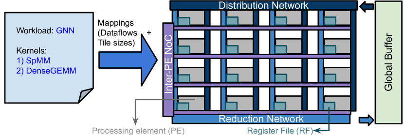
Figure 1: Spatial Accelerator

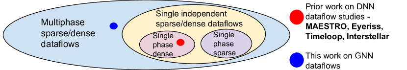
Figure 2: Map space of our work on GNN dataflow studies is a superset of that of prior works on DNN dataflow studies - MAESTRO [8], Eyeriss [7], Timeloop [9] and Interstellar [10].

GNNs are becoming increasingly popular because of their ability to accurately learn representations from graph-structured data to solve graph/node classification, graph generation, and link prediction problems [15]. Example applications include item recommendation [16], molecular feature extraction [17] and natural language processing [18]. GNN inference runtime is dominated by two phases: (1) Aggregation and (2) Combination [19]. Aggregation is an SpMM computation with irregular, workload dependent accesses of data. Combination computations can be cast as GEMMs, similar to dense DNNs.

Several recent works on GNN acceleration [19, 20, 21, 22, 23, 24] have demonstrated the challenges with getting high performance for GNNs from commodity CPUs, GPUs, and DNN accelerators. These challenges arise from (i) extremely high amounts of sparsity in the Aggregation phase (over 99% as compared to 70-80% in modern DNNs), and (ii) diverse data reuse opportunities within and across these phases. These works have also demonstrated that GNNs offer opportunities for acceleration by crafting specialized dataflows for extracting reuse both within and across the phases. Unfortunately, most of these prior works propose building specialized GNN accelerator ASICs with heavy co-design of a specific GNN dataflow and its hardware microarchitecture, which limits their applicability as graph datasets and GNN algorithms evolve. In contrast, this is the first work, to the best of our knowledge, that provides a qualitative and quantitative analysis of the design-space of various inter-phase and intra-phase dataflow strategies for mapping GNNs over flexible spatial accelerators.

This work makes the following contributions:

(i) Taxonomy: We propose a succinct taxonomy to classify various inter-phase and intra-phase dataflows to describe the possible pipelining strategies employed by GNN accelerators. This taxonomy expresses: (1) Aggregation intra-phase dataflow, (2) Combination intra-phase dataflow, (3) Inter-phase strategy, and (4) phase ordering. Rather than targetting a specific GNN accelerator where the dataflow choices might be limited due to its microarchitecture [19, 21, 20], or directly compare two different GNN accelerators where it would become hard to tease apart the performance difference due to dataflow versus microarchitecture, we target a templated flexible spatial accelerator substrate [5, 6] over which any dense/sparse dataflow that our taxonomy describes can be run.

(ii) Qualitative Analysis and Analytical Framework: Using the taxonomy, we explore various factors that affect the runtime and the energy of these dataflow strategies such as spatial/temporal mapping choices of various dimensions in the intra-phase, the pipelining granularity in the inter-phase, and tile sizes. We encode these into a framework called OMEGA.

(iii) Quantitative Analysis: Using OMEGA, we study the impact of graph properties (such as number of vertices, edges, features) on dataflow choices. We also analyze the impact of hardware parameters, for example, low distribution and reduction bandwidth, and issues of load balancing in pipelining.

(iv) Architectural Insights: We demonstrate the benefits of reconfigurable dataflow accelerators for multiphase computation as opposed to GNN accelerator ASICs given the interdependence of dataflows.

This work explores the design-space of pipelined dataflows with both sparse and dense phases, and proposes the OMEGA framework to model the cost of these dataflows. The insights from this work can extend to other ML and HPC workloads with multiphase kernels [2], [14]. We envision that the taxonomy will formalize the design-space of multiphase dataflows which will enable better mapping optimizers for ML and HPC workloads. Moreover, the future mapping optimizer can use OMEGA framework as a cost-model for multiphase dataflows. The insights from this work would also help the architects make informed design decisions, thus enabling a richer HW/SW co-design for future ML and HPC accelerators.

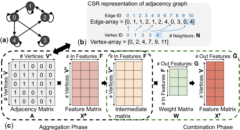
Figure 3: (a) Example graph, (b) CSR representation of the adjacency matrix, (c) computations. Note: V* can be represented as neighbors(N) if it is represented in CSR format. Also, figure assumes computation order Aggregarion to Combination ((AX⁰)W). For Combination to Aggregation (A(X⁰W)), intermediate matrix is V$\times$G.

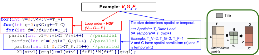
Figure 4: Example showing compact notation for the loop-nest for Combination phase dataflow and an example tiling strategy for that dataflow. See Fig 3 for dimension and matrix notations. Similar loop ordering and tiling notation applies to Aggregation.

II Background and Related Work

II-A GNN Computation

An input graph is represented by G(V, E) with V vertices and E edges. A graph can also be represented as an adjacency matrix which represents the connectivity of the graph. Matrix representations are common, since dense/sparse matrix multiplication has been the prime target of spatial accelerators.

Recent works show that the main computation bottlenecks of various GNN algorithms like GCN [13], GraphSage [25], GINConv [26] can be broken down into two phases: Aggregation and Combination [19]. GCNs allow either phase to precede the other while some algorithms like GraphSAGE perform Aggregation before Combination. The Aggregation phase involves the addition of the feature vectors of the neighboring nodes in the graph. This leads to irregular accesses of data due to the irregular degree distribution in the graphs of interest and, as a result, irregularity in the neighbor locations of a particular vertex in a given dataset. The Aggregation phase can be mapped as sparse matrix$\times$dense matrix multiplication (SpMM) with the highly sparse adjacency matrix being the main source of irregular accesses. The Combination phase is a feature reduction phase. This phase is dense with regular GEMM computation.

Fig. 3a) shows an example graph with five vertices and eleven edges, including self loops and Fig. 3c) shows the adjacency matrix representation of the graph. Fig. 3b) is the Compressed Sparse Row (CSR) representation of the graph’s adjacency matrix. For CSR representation, the neighbors of a particular vertex are stored back-to-back. Because most graphs are extremely sparse ($>$ 99% sparsity) [27], CSR is often used as the graph representation [19, 20], and is what we assume in this work. As labeled in Fig. 3c), A represents the adjacency matrix, X represents the feature matrix, and W represents the weight matrix. Any computation with A is a part of the Aggregation phase, and any computation with W is a part of the Combination phase. Other variables include: V (# vertices), F (# input features), G (# output features), and N (# of neighbors of a vertex).

II-B GNN Accelerators

Several GNN accelerator ASICs have been proposed [28, 21, 19, 20, 22, 24, 23, 29, 30], each implementing a specific dataflow which is heavily co-designed with the microarchitecture. The dataflows from these accelerators form a subset of the design-space that we explore. GCNAX [29] proposes a flexible GCN accelerator with the ability to choose between some dataflows to optimize for energy. However, GCNAX primarily targets off-chip dataflows with a small global buffer and 16 PEs, while our work focuses on on-chip dataflow strategies for large programmable spatial accelerators with high parallelism opportunities.

II-C Dataflow Analysis

There have been several efforts to understand and classify dataflows for DNNs such as Timeloop [9], Interstellar [10], and MAESTRO [8]. However, as Fig. 2 shows, these works focus only on dataflows for single dense layers, forming a subset of dataflows that we study in this work (which includes pipelining and multi-phase sparse-dense dataflows).

III GNN Dataflow Taxonomy

In this section, we discuss the GEMM/SpMM dataflows within an individual phase (Intra-phase dataflows) and the overall dataflow with both phases (Inter-phase dataflows).

Notation. We use the notations from Fig. 3 for the matrices and the dimensions for the rest of the paper. Fig. 4 presents the succinct notations we use for describing the dataflow of a single phase, without writing out its full loop-nest. It describes the loop order (i.e., order of temporal loops) and the spatial parallelism choices which are determined by the tile sizes. In this paper, tile size (T_Dim) represents spatial loop tiling and it refers to the number of elements of a dimension mapped in parallel across PEs. For instance, T_F is the number of input features (F) processed in parallel across PEs. Here s and t in the subscript represent whether a dimension Dim is spatial (which means T_Dim>1) or temporal (T_Dim=1). Also, V and F dimensions are used in both the phases so we use T_V_CMB to describe T_V in Combination phase and T_V_AGG for Aggregation.

Table I discusses the implication of the loop order and the spatial parallelism of the dimensions on data movement for three popular 2D GEMM dataflows. Next, we describe various dataflow choices and the taxonomy to describe the intra-phase and the inter-phase dataflows.

TABLE I: Example 2D GEMM dataflow choices for combination and their hardware implications. The subscript $\mathbf{s}$ on two dimensions represents spatial mapping (i.e., unrolling) of those dimensions across the rows and columns of the accelerator (in a tiled manner), while $\mathbf{t}$ represents temporal mapping. "Stationary" means that the matrix is inside the PEs while "streaming means" that the matrix is streamed from GB.

Dataflow	Implication of Loop Order	Implication of Spatial Dimensions
VsGsFt	Output (VG) stationary, Intermediate matrix (VF) and Weights (FG) stream every cycle	Spatial multicast of VF and FG every cycle. Temporal reduction of partial sums within each PE.
GsFsVt	Weight (FG) stationary, Intermediate matrix (VF) streams every cycle	Spatial multicast of VF every cycle. Spatial reduction of partial sums across PEs
VsFsGt	Intermediate matrix (VF) stationary, Weight (FG) streams every cycle	Spatial multicast of FG every cycle. Spatial reduction of partial sums across PEs

III-A Intra-phase Dataflow

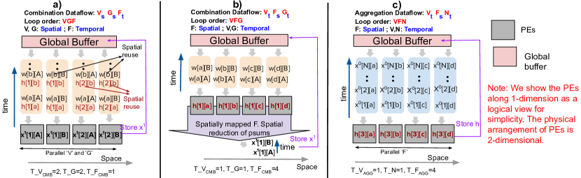
Figure 5: Examples of different intra-phase dataflows. a) Combination dataflow: $V_{s}G_{s}F_{t}$, b) Combination dataflow: $V_{t}F_{s}G_{t}$ c) Aggregation dataflow: $V_{t}F_{s}N_{t}$. See Fig. 3 for matrix and dimension notations. Input feature indices $x^{0}[n=1,2..][f=a,b...]$, Weight indices: $w[f=a,b..][g=A,B..]$, Intermediate indices: $h[v=1,2...][f=a,b..]$, Output feature indices: $x^{1}[v=1,2][g=A,B]$.

III-A1 Combination Dataflow

Fig. 5a) and b) show examples of Combination dataflows. In Fig. 5a), V$\times$F matrix ($h[v][f]$) and F$\times$G matrix ($w[f][g]$) stream from the buffer into the PEs. The input features vary each cycle, and thus the dimension is temporally mapped and their T_F_CMB=1 due to no spatial parallelism. The other dimensions are spatial since they have parallelism. The tile sizes T_V_CMB and T_G are 2, since two vertices ‘1’ and ‘2’ and two output features ‘A’ and ‘B’ are parallelized. Also, ‘w’ and ‘h’ are spatially multicasted in this example. This results in V_sG_sF_t. The reduction is temporal which can be achieved by the accumulators inside the MACs. As another example, Fig. 5b) shows a Combination dataflow in which different features are mapped in parallel. V$\times$F matrix is present in the RF. F$\times$G matrix is streamed from the buffer into the PEs. Different partial sums resulting from different features “a-d” are reduced spatially which can be done through a linear chain or adder tree [8]. This results in V_tF_sG_t with T_V_CMB=T_G=1 and T_F_CMB=4.

III-A2 Aggregation Dataflow

Fig. 5c) illustrates an example of an Aggregation dataflow. Sparsity gets encoded as N in taxonomy. As Fig. 3b shows, N can be encoded in CSR, in which all of the neighbors are stored back-to-back. The example shows V as the outermost loop, and is temporal. The next loop contains F which has spatial parallelism ($s$). In the innermost loop, N is temporal, thus temporal reduction is required. This results in V_tF_sN_t.

III-B Inter-phase Dataflow

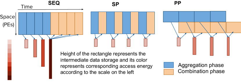
Figure 6: Space-Time representation of Inter-phase dataflows along with Intermediate data movement. If the intermediate data exceeds the storage capacity of the on-chip buffers, it needs to move back and forth between memory which adds energy costs.

Although each phase can use any intra-phase dataflow, as described above, the dataflow choice for one can affect the other. This opens up a design-space for inter-phase dataflow. This part of the dataflow is important as it determines the number of memory accesses required to move data from one phase to the next. Fig. 6 presents the types described below.

III-B1 Sequential (Seq)

Seq is the simplest inter-phase dataflow where the two phases are run sequentially. All the outputs of the first phase are stored in the global buffer (and moved to DRAM if the size of the global buffer is insufficient) and then loaded back to the PEs for the next phase.

III-B2 Sequential Pipeline (SP)

SP is similar to Seq but it splits the computation of Aggregation and Combination phases into small steps, which are then interleaved over time on the accelerator’s PEs. As Fig. 6 shows, it is possible to reduce the data movement between Aggregation and Combination phases depending on the intra-phase dataflows. Specifically, the output data generated by one step can be kept stationary within PEs’ local registers rather than going into a global buffer or DRAM. Fig. 7b) shows an example of this. The Aggregation dataflow is same as the dataflow in Fig. 5c) and the Combination dataflow is same as the dataflow in Fig. 5b) (T_F in both phases is 8). In each pipeline step: (a) a part of the intermediate matrix is computed by the Aggregation phase and is stored within the RF of a PE. (b) Weights are streamed over that part of the intermediate matrix to produce a part of the output matrix.

III-B3 Parallel Pipeline (PP)

PP is when both phases are allocated onto parallel units (i.e., group of PEs) within an accelerator at the same time. The size of these parallel units can be fixed (e.g., HyGCN  [19]) or flexible (e.g., AWB-GCN  [20]), depending on the flexibility within the accelerator substrate. For PP, it is critical to balance the production and consumption rate to reduce stalls. An intermediate ping-pong buffer and NoC. are needed to send data from one phase to the next. This is similar to the typical workflow for a more general accelerator such as GraphCore [3]. Fig. 7a) shows an example of PP dataflow. In this example, the Aggregation dataflow is same as the dataflow in Fig. 5c) and the Combination dataflow is same as the dataflow in Fig. 5a). In each pipeline step ‘n’, the left half performs Aggregation and the right half parallelly performs Combination on the part of the intermediate matrix which was produced by Aggregation in the previous step ‘n-1’.

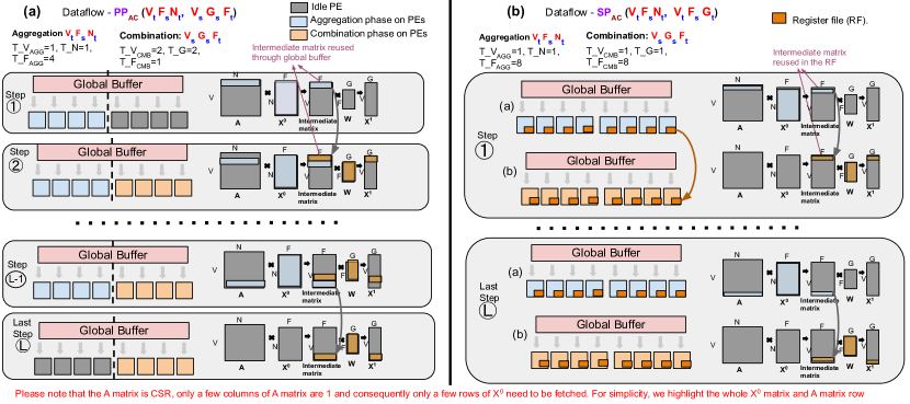
Figure 7: Step-by-step execution of inter-phase dataflows. a) $PP_{AC}(V_{t}F_{s}N_{t},V_{s}G_{s}F_{t})$ b) $SP_{AC}(V_{t}F_{s}N_{t},V_{t}F_{s}G_{t}{t})$. Here, “step” refers to duration in which producer writes a part of the intermediate matrix and consumer reads a part of the intermediate matrix. We show the allocation of PEs to the phases and the parts of the matrices computed in each step. See Fig. 3 for matrix and dimension notations. Dataflow notation is described in Section III-C. The intra-phase dataflows are shown in detail in Fig. 5.

TABLE II: Characterizing the design-space of GNN dataflows. Note that any direction will affect the aggregation and combination dimension variables, but similar concepts apply. Subscripts s, t, x mean spatial, temporal, either spatial or temporal respectively.

Row	Inter Phase	Order - Aggregation, Combination	Intermediate Global Buffer	NoC/PE support	Example & Order	Remarks
1	Sequential (Seq)	ANY-All pairs	✓	Intra-phase	TPU [31] Eyeriss [7] (any direction)	Similar to running one DNN layer at a time. The outputs of one phase get stored in the memory and rescheduled back onto the PEs.
2	Sequential Pipeline (SP)	AC - VxFxNt, VxFxGt AC - FxVxNt, FxVxGt CA - NxFxVt, VxGxFt CA - FxNxVt, GxVxFt	✗	Local buffer inside PEs to accumulate data	EnGN [21] (any direction)	SP-Optimized: Avoids GB accesses, as output data of one phase is stationary in the PE RF, and can be used as input for the next phase. For agg->cmb, T_VAGG=T_VCMB and T_FAGG =T_FCMB and reduction is temporal as the data is always inside in-place buffers.
3		Same as rows 4-9	✓	Intermediate outputs stored in GB.	(any direction)	SP-Generic: There will be a buffer/ setup delay between aggregation and combination phases to remap the output data to a new location.
4	Parallel Pipeline (PP)	AC - VxFxNx, VxFxGx AC - FxVxNx, FxVxGx	✓	NoC connecting Agg and Cmb units to intermediate buffer.	(agg ->cmb)	Element(s) wise granularity: Element(s) of the intermediate matrix indexed by V,F can be pipelined.
5		AC - VxFxNx, VxGxFx AC - VxNxFx, VxGxFx AC - VxNxFx, VxFxGx	✓	NoC connecting Agg and Cmb units to intermediate buffer.	HyGCN [19] Auten et al. [24] (agg ->cmb)	Row(s) wise granularity:Row(s) of the intermediate matrix indexed by V can be pipelined. HyGCN allocates a fixed number of PEs, which may lead to stalls. (combination engine idle waiting). HyGCN dataflow-$PP_{AC}(V_{x}F_{s}N_{t},V_{s}G_{s}F_{t})$
6		AC - FxVxNx, FxGxVx AC - FxNxVx, FxGxVx AC - FxNxVx, FxVxGx	✓	NoC connecting Agg and Cmb units to intermediate buffer.	(agg ->cmb)	Column(s) wise granularity: Column(s) of the intermediate matrix indexed by F can be pipelined.
7		CA - NxFxVt, VxGxFt CA - FxNxVt, GxVxFt	✓	NoC connecting Agg and Cmb units to intermediate buffer.	(cmb ->agg)	Element(s) wise granularity: The order should be (NFV, VGF) or (FNV, GVF). V$\times$G matrix after Cmb becomes N $\times$ F for Agg.
8		CA - NxVxFx, VxGxFx CA - NxVxFx, VxFxGx CA - NxFxVx, VxFxGx	✓	NoC connecting Agg and Cmb units to intermediate buffer.	(cmb ->agg)	Row(s) wise granularity
9		CA - FxVxNx, GxVxFx CA - FxVxNx, GxFxVx CA - FxNxVx, GxFxVx	✓	NoC connecting Agg and Cmb units to intermediate buffer.	AWB-GCN [20] (cmb ->agg)	Column(s) wise granularity: AWB-GCN enables a flexible allocation of PEs for different phases to match production and consumption rates. AWB-GCN dataflow- $PP_{CA}(F_{s}N_{t}V_{s},G_{t}F_{t}V_{s})$

III-C Complete Description of GNN Dataflow

Given the dataflow types described above, we use the following template to describe a complete dataflow:

<Inter>_<order>(<AggIntra>, <CmbIntra>)

<Inter> represents the inter-phase dataflow, <order> represents the computation order (Aggregation to Combination is AC, Combination to Aggregation is CA). <AggIntra> represents the Aggregation phase intra-phase dataflow, and <CmbIntra> represents the Combination phase intra-phase dataflow.

Table II uses our taxonomy to enumerate and characterize the space of dataflow choices for mapping the Aggregation and Combination loops, including the hardware structures required for supporting that dataflow. To keep the table compact, we add a subscript x to indicate that the dimension could be spatial or temporal. This leads to a total of 6,656 choices purely from the product of all feasible loop orders, parallelism choices, and phase order across the three inter-phase choices. Note that for each dataflow choice, the tile sizes (T_Dim) are also parameters which can put the actual number of possible mappings in the trillions [9]. We observe in Table II and Section IV that the loop orders and the tile-sizes of two phases are interdependent for SP and PP dataflows. Thus we formalize the non-trivial space of multiphase GNN dataflows.

For the purposes of analysis, in Table II we explicitly list sets of interesting dataflows (some of which existing accelerators have leveraged) with the remarks highlighting their key characteristics. As an example, the HyGCN [19] accelerator’s dataflow can be succinctly described as: $\small PP_{AC}(V_{x}F_{s}N_{t},V_{s}G_{s}F_{t})$ In fact, the dataflow shown in Fig. 7a) is the same as that used by HyGCN [19]. However, note that HyGCN microarchitecture employs separate dedicated SIMD and Systolic engines respectively for Aggregation and Combination, along with a dedicated buffer between them for intermediate values. The dataflow is tied to the microarchitecture; in contrast, Fig. 7a) runs the HyGCN dataflow on a programmable spatial accelerator by configuring different sets of PEs to run the Aggregation and Combination dataflows described earlier in Section III-A and staging the intermediate values through the flexible partitions in the programmable scratchpads.

Hardware support for dataflows. We note that each dataflow may require different levels of support from the hardware. For the intra-phase dataflows, support for multicasts and reductions (either spatially via a store-and-forward or temporally via a read-modify-write register within PEs) may be needed [8]. For the inter-phase dataflows, Table II lists the NoC and PE support needed for each dataflow. We discuss the implications of hardware parameters in detail in Section V-C.

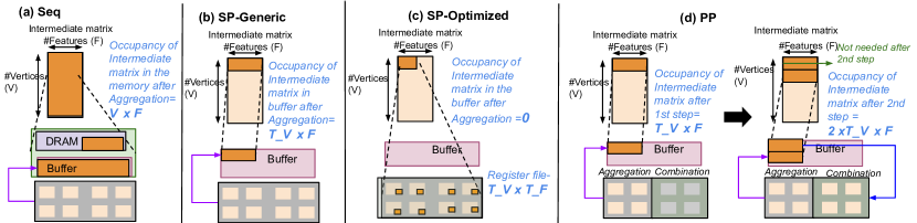
Figure 8: Intermediate buffering in Inter-Phase dataflows – AC computation order is assumed.

IV Qualitative and Analytical Analysis

In this section, we present a qualitative analysis of the trade-offs of various inter-phase choices and their runtime and storage implications. Table III summarizes the runtime and intermediate buffering requirements for inter-phase dataflows that we derive here. We also focus on the intra-phase dataflow implications on inter-phase dataflows where both the phases are interdependent. Thus multiphase dataflow space is non-trivial. For the analysis in this section, we focus on AC computation order, but the same concepts apply to CA.

IV-A Sequential Dataflow

Recall that in sequential dataflow, the phases simply run one after the other using any intra-phase dataflow. The overall latency is the sum of latencies of individual phases. The entire intermediate matrix is first written to the memory by the first phase and then read from the memory by the second phase. Hence, as Fig. 8a) shows, the intermediate matrix occupancy in the memory is simply the number of elements of Intermediate matrix which is V$\times$F. Such amount of data cannot be stored on-chip for large graphs, as Fig. 6 shows, and would incur higher energy than the other inter-phase dataflows.

IV-B Sequential Pipeline (SP)

In the Sequential pipeline dataflow, a few elements of the first phase are computed and the second phase is applied and this is repeated in an interleaved manner over time. As Fig. 6 shows, this reduces the intermediate matrix footprint and naturally gives an energy advantage over Seq by avoiding expensive memory accesses down in the memory hierarchy (including DRAM).

SP-Generic. This can be considered a naïve implementation for the SP dataflow. As Fig. 8b) shows, for SP-Generic dataflow, the intermediate data produced in the Aggregation phase is written by the PEs to the global buffer, and then read from there for computing the Combination phase. Thus, the intermediate storage required is equal to the number of elements pipelined which we define as Pel. The intermediate data is broken down into granularities which we describe in detail in Section IV-D. The feasible loop orders are shown in row 3 of Table II, which is equivalent to the PP loop orders shown in rows 4-9. The total runtime of SP-generic is similar to the sequential dataflow, although the energy would be lower by avoiding the transfer of the Aggregation outputs to memory.

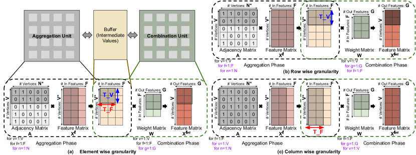
Figure 9: PP strategies with different granularities: a) Element(s) wise a) Row(s) wise and a) Column(s) wise for the phase order AC.

SP-Optimized. In order to save both energy and latency, we can select a subset of intra-phase dataflows for Aggregation and Combination such that the outputs generated by Aggregation can stay local within the PEs’ registers and be reused directly by the Combination phase. This avoids writing this intermediate data up the memory hierarchy to the buffer and reading it again. These dataflows are SP_AC(V_xF_xN_t,V_xF_xG_t) and SP_AC(F_xV_xN_t,F_xV_xG_t) for Aggregation to Combination order and are shown in Row 2 of Table II. In this dataflow, the requirement is that the loop order pair for Aggregation and Combination phases should be (VFN, VFG) or (FVN, FVG). After the first iteration of temporal loop-nest of V,F is finished with all neighbors reduced, the accumulated data remains in the MAC units and then dimension G is streamed over it. Moreover, corresponding T_Dimensions for both Aggregation and Combination would be same (ie T_V_AGG=T_V_CMB and T_F_AGG=T_F_CMB) since the same intermediate data stored in the PEs by the first phase is processed by the second phase. Also, since the data should be available for consumption locally in the processing elements, the reduction must be temporal (T_N=1). The advantage of SP-optimized is reduced buffer accesses and reduced buffer requirement, since the data to be used in the second phase is directly used inside the PEs, as also shown in Fig. 8c). Moreover, it saves the latency and memory read overhead of loading the data into PEs. An instance of SP-Optimized is used by the EnGN [21] accelerator.

IV-C Parallel Pipeline (PP)

Parallel pipeline dataflow divides the accelerator into two engines, with one engine feeding the other engine spatially. As Fig. 8d) shows, the intermediate data is broken down into small granularities and the data is processed in a pipelined manner. For example, if granularity is a single row of the intermediate matrix, then the Aggregation phase computes and writes the data corresponding to the n^th row and in parallel, the Combination phase reads and processes data corresponding to the (n-1)^th row. To facilitate this, intermediate ping-pong buffers are required. As Fig. 8d) shows, the amount of intermediate buffering required is twice the number of elements of the intermediate matrix pipelined. We refer to the number of elements being pipelined as Pel. Thus the amount of intermediate storage used is $2\times Pel$, $Pel$ for each phase. The runtime of one pipeline step is equal to the runtime of the slower phase for producing Pel elements. The total runtime is the sum of runtimes of individual steps $sum(max(t_{AGG},t_{CMB})_{Pel})$.

IV-D Granularities for SP-Generic and PP

We discuss three types of granularities at which the intermediate matrix can be broken into pipeline steps for PP and SP-Generic dataflows. Rows 4-9 in Table II show all feasible loop orders for all possible granularities and phase orders.

Element. Element(s)-wise granularity involves tiles of a few elements being processed in a pipelined manner rather than the whole dimensions. Fig. 9a) shows an example of element(s)-wise granularity PP_AC(V_xF_xN_x, V_xF_xG_x). For each element(s) which is (are) indexed by V and F, the inner-most loop (N) of Aggregation reduces all the neighbors for a given tile of vertices and features to be reduced and, in parallel, the innermost loop of Combination computes G for the previous tile of vertices and features. The amount of buffering is 2$\times$Pel for PP datalow and Pel for SP-Generic. $Pel$ = T_V_max$\times$T_F_max.

Row. In row(s)-wise granularity, the whole row(s) of the intermediate matrix is (are) considered instead of a few elements in a row. The number of rows that are pipelined is T_V_max. So Pel = T_V_max$\times$F. Fig. 9b) shows an example loop order (VFN, VGF) for row(s) wise granularity for PP dataflow for phase order Aggregation to Combination. For each set of rows indexed by V, the inner two loops F and N compute Aggregation, and in parallel, the two innermost loops G and F compute Combination for the previous row(s). An instance of this dataflow is used in HyGCN [19].

Column. In column(s)-wise granularity, the whole column(s) of the intermediate matrix is (are) considered instead of a few elements in a column. The number of columns that are pipelined is T_F_max. So Pel = T_F_max$\times$V. Fig. 9c) shows an example loop order (FVN, FGV) for column(s) wise granularity for PP dataflow for phase order Aggregation to Combination. Each column of the aggregated matrix is indexed by F while the inner two loops compute the computations corresponding to columns in a pipelined manner.

Table III summarizes the runtime and buffering requirements for the different inter-phase dataflows discussed before.

TABLE III: Runtime and buffering requirements for Dataflows

Inter-phase dataflow	Intermediate Buffering	Runtime
Seq	V$\times$F	tAGG+tCMB
SP-Generic	$Pel$	tAGG+tCMB
SP-Optimized	0	tAGG+tCMB-tload
PP-Element	2$\times$T_Vmax$\times$T_Fmax	sum(max(tAGG,tCMB)Pel)
PP-Row	2$\times$T_Vmax$\times$F	sum(max(tAGG,tCMB)Pel)
PP-Column	2$\times$V$\times$T_Fmax	sum(max(tAGG,tCMB)Pel)

V Quantitative Analysis and Case Studies

In this section, we do a deep dive into the performance and energy of different GNN dataflows. We also perform case studies on hardware implications.

V-A Experimental Methodology

V-A1 Cycle-Accurate Simulation Framework

In order to carry out a detailed evaluation of various dataflows, we built a cycle accurate simulation framework called OMEGA (Observing Mapping Efficiency over GNN Accelerators) around STONNE simulator[32]. Fig. 10 shows the overview of the OMEGA framework. STONNE simulator models the flexible accelerators MAERI[6] and SIGMA[33], and the hardware models have been extensively validated against their RTLs.

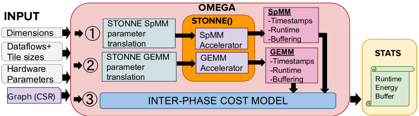
Figure 10: OMEGA framework toolflow.

It consists of reconfigurable networks-on-chip for operands (e.g., inputs, partial sums and weights) distribution, operands multiplication, and output reduction (e.g., addition) allowing us to study different tile sizes. The simulator uses a single-cycle distribution network used in the MAERI accelerator. The STONNE framework also supports CSR decoding and indexing logic to run SpMM in addition to GEMM to compute both phases. To implement inter-phase dataflows, we built an inter-phase cost model that analytically computes the runtime, buffering, and energy statistics of inter-phase dataflows using statistics from individual phases. The inter-phase cost model uses an analytical model to compute results for inter-phase dataflows from intra-phase dataflows based on the analysis in Section IV. Some of the example equations are shown in Table III. Some dataflows like PP require timestamps for the portions of outputs computed for both the phases, which are collected at the granularity of $Pel$.

V-A2 Datasets

We evaluate the GNN dataflows for the target datasets described in Table IV. These are standard datasets representing workloads from multiple domains like biochemistry, citation networks, and social networks [27, 34]. We evaluate one batch of 64 graphs for graph classification workloads (batch of 32 graphs for RedditBIN) and we evaluate node classification datasets Citeseer and Cora. The large graph sets are generally sliced to fit on-chip [19, 21]. Large graph classification datasets can be batched such that the graphs fit on-chip. For this work, there is sufficient on-chip buffering for a batch of graph classification datasets and for node classification datasets. We characterize on-chip data movement and runtime of the GNN dataflows since our aim is to study the behavior of these dataflows on spatial accelerators. Based on the matrix dimensions and sparsity, we divide the workloads into 3 categories: high number of edges/vertices and relatively low features/vertices (HE), high features/vertices and relatively lower edges/vertices (HF), and low edges/vertices and low number of features/vertices (LEF).

V-A3 Evaluation Parameters

Unless specified otherwise, we assume the number of PEs to be 512 with 64B banked RF in each PE. We also assume sufficient distribution and reduction bandwidth to ensure that the data is received from (or sent to) all the PEs without any stalls. The tile sizes are chosen such that they satisfy the dataflow description in Table V and the static utilization is nearly 100% of the PEs. For PP dataflow, unless otherwise mentioned, half the PEs perform Aggregation phase and half the PEs perform Combination phase.

TABLE IV: Datasets information. First part for graph classification, bottom part for node classification – ‘*’ means that indicator vectors were used in place of features.

Name	#Graphs	#Nodes(av)	#Edges(av)	#Features	Category
Mutag	188	17.93	19.79	28*	LEF
Proteins	1113	39.06	72.82	29 (full)	LEF
Imdb-bin	1000	19.77	96.53	136*	HE
Collab	5000	74.49	2457.78	492*	HE
Reddit-bin	2000	429.63	497.75	3782*	HF
Citeseer	1	3327	9464	3703	HF
Cora	1	2708	10858	1433	HF

TABLE V: Dataflow configurations for evaluation.

Dataflow Configuration	Name	Distinguishing Property
SeqAC(VxFxNt,VxGxFx)	Seq1	Temporal Aggregation (T_N=1)
SeqAC(VxFxNs,VxGxFx)	Seq2	Spatial Aggregation (T_N>1)
SPAC(VxFsNt,VxFsGx)	SP1	Temporal Aggregation & high T_F
SPAC(VsFxNt,VsFxGx)	SP2	Temporal Aggregation & high T_V
SPAC(VsFxNt,VsFxGx)	SPhighV	SP dataflow; extremely high T_V
PPAC(VxFxNt,VxGxFx)	PP1	Temporal Aggregation &
		Granularity of lower rows
PPAC(VxFxNs,VxGxFx)	PP2	Spatial Agg. & low granularity
PPAC(VxFxNt,VsGxFx)	PP3	Temporal Agg. & high granularity
PPAC(VxFxNs,VsGxFx)	PP4	Spatial Agg. & high granularity

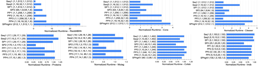
Figure 11: Runtimes of Dataflows normalized to Seq1 for GCN algorithm. PE Utilization is close to 100%. The values in the brackets are tile sizes for each dimension, represented as (T_V_AGG,T_N,T_F_AGG,T_V_CMB,T_G,T_F_CMB).

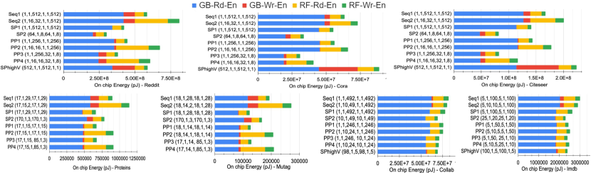
Figure 12: On-Chip buffer access energies of dataflows, GB is Global Buffer and RF is local (PE) register file. Size of the Intermediate buffer for PP depends on the pipelining granularity. The values in the brackets are tile sizes for each dimension, represented as (T_V_AGG,T_N,T_F_AGG,T_V_CMB,T_G,T_F_CMB).

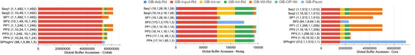
Figure 13: Global Buffer breakdown for Mutag and Citeseer, Adj-Adjacency matrix, Inp-Input matrix, Int-Intermediate matrix, Wt-weight matrix and Op-output matrix, Psum-partial sum accesses. The values in the brackets are tile sizes for each dimension, represented as (T_V_AGG,T_N,T_F_AGG,T_V_CMB,T_G,T_F_CMB).

V-B Comparison of Dataflows

We compare the performance and energy of the GNN dataflows. We evaluate the representative dataflow configurations shown in Table V.

V-B1 Performance

Fig. 11 shows the runtimes of various dataflows. Our observations are as follows:

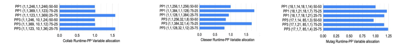
Figure 14: Runtimes with different PE allocation to phases. Label represents the dataflow and the PE allocation ratio PE_AGG-PE_CMB. Runtimes are normalized to 50-50 low granularity. The values in the brackets are tile sizes for each dimension: (T_V_AGG,T_N,T_F_AGG,T_V_CMB,T_G,T_F_CMB).

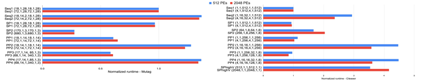
Figure 15: Runtime for 2048 and 512 PEs. Runtimes are normalized to that of Seq1 in each case. The values in brackets are tile sizes-(T_V_AGG,T_N,T_F_AGG,T_V_CMB,T_G,T_F_CMB).

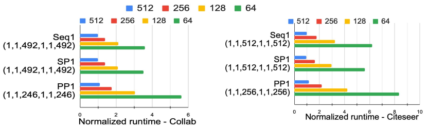
Figure 16: Runtime normalized to that of Seq1 for 512 elements. Legend represents the number of elements that can be sent to or received from global buffer in parallel. The values in brackets are tile sizes-(T_V_AGG,T_N,T_F_AGG,T_V_CMB,T_G,T_F_CMB).

• SP2 (High T_V) performs well in most cases since parallelization of the vertices leads to reduced redistribution overhead. However, for HF datasets, extremely high T_V can lead to delays since the performance is limited by a dense row (with large number of non-zeros) as demonstrated in SPhighV dataflow. Such dense row is referred to as "evil row" in AWB-GCN [20].

• For Collab and Imdb (HE category) spatial Aggregation, in general performs much better than temporal, because they are densely connected. For other datasets, since they are sparse, optimal T_N is low.

• Mutag and Proteins have great performance despite extremely high T_V, since these don’t have evil rows.

• For the Collab dataset, PP performs worst due to poor load balancing between Aggregation and Combination.

V-B2 Energy

Figure 12 shows the energy consumed by various dataflows across workloads and Fig. 13 shows global buffer accesses. The energy difference comes due to differences in the number of accesses across the memory hierarchy. We assume the energy of a global buffer (GB) access to be 1.046pJ (1MB/bank) and the energy of a local PE register file (RF) access to be 0.053pJ based on the energy model from Dally et al. [35]. For PP dataflow, we assume that there is a separate ping-pong buffer partition for intermediate data and the its size depends on the capacity required based on Table III. Our observations are as follows:

• Energy is dominated by GB reads followed by RF reads.

• In Collab (HE category), input GB accesses dominate, in Cora (HF), weight GB accesses dominate. Mutag (LEF) has best percentage of accesses reduced due to reuse.

• In PP dataflow, we observe lower energy compared to Seq since the energy of memory accesses from smaller intermediate buffer partition is less. SP has no intermediate matrix accesses resulting in low energy.

• SP2 has low energy but SPhighV has higher energy due to the partial sum accesses due to low T_F, especially for HF datasets like Cora.

V-C Case Study: Hardware Parameter Implications

1) PP: Load balancing. In PP dataflow, the delay is decided by the slower phase. Therefore load balancing is critical. Fig. 14 shows the performance of different allocations of PEs to the phases for different pipeline granularities. Collab has higher density (HE category) hence slow Aggregation, therefore 25-75 performs poorly. For Mutag (LEF category), 50-50 is the best allocation scheme amongst the three allocation schemes Since, Citeseer is sparse and has high number of features (HF category), the Combination phase is slower, therefore 75-25 allocation performs poorly.

2) Scalability of the performance across dataflows. Fig 15 shows the performance of the dataflows for an accelerator with 512 and 2048 PEs for Mutag and Citeseer datasets. Tile sizes are chosen to maximize the static utilization. We observe that the runtimes normalized to the Seq1 dataflow are similar in case of 512 and 2048 PEs, especially for dataflows with low runtimes. Therefore, the relative performance of dataflows generalizes for different scales of acceleration.

3) Implications of low bandwidth. For Section V-B, we assumed sufficient on-chip distribution and reduction bandwidth to ensure that the data is received/sent without stalls. However, a low global buffer distribution bandwidth and a low reduction bandwidth lead to stalls affecting the performance. Fig. 16 shows the performance implications of reducing the bandwidth for different inter-phase dataflows. Runtime reduces with the decrease in the bandwidth and PP dataflow suffers the most since the bandwidth is shared between the two phases.

V-D Architectural Insights: Flexibility for Efficient Pipelining

In this section, we show that flexible accelerators do not only support multiple dataflows but also support efficient pipelining given the interdependence of Aggregation and Combination dataflows in SP and PP. We discuss flexibility features needed in an accelerator to support efficient pipelining.

SP-Optimized: In this dataflow, T_V_AGG=T_V_CMB and T_F_AGG=T_CMB. Also, in order to retain the intermediate matrix locally in PE, T_N=1 (temporal reduction in Aggregation). For Combination, T_F_CMB determines the spatial reduction. A rigid architecture with only spatial reduction cannot map SP-Optimized. A rigid architecture with only temporal reduction can map only one instance with tile sizes T_F=T_N=1 which implies that only V is distributed parallelly. This dataflow is SPhighV. We observe from Fig. 11 and 12 that this dataflow has a huge runtime due to performance being limited by the sparse rows. It also has a huge energy value due to the overhead of writing and reading partial sums. Therefore, configurability of tile sizes is essential given the interdependence of phases.

PP dataflow: We observed in Fig. 14, how critical load balancing is, and that the optimal allocation to a phase can change depending on workload sparsity and dimensions. Using a rigid substrate with two distinct sub-accelerators like HyGCN [19] causes load imbalance for certain workloads. Load balancing also requires tile sizes such that stalls are minimized due to the slower phase. Therefore flexible resource allocation and configurability of tile sizes are essential for mapping PP efficiently.

Flexibility features: Mapping SP and PP dataflows efficiently requires configurable tile sizes and flexible resource allocation. Moreover as Section V-B shows, flexibility to choose from SP and PP according to the workload leads to an optimal dataflow. These features add up to a programmable spatial accelerator [2, 4, 3, 6, 5]. However, there is no additional cost for a programmable spatial accelerator running pipelined dataflows compared to running single phase dataflows. Therefore flexibility provides more benefit per cost for mapping multiphase kernels than independent kernels.

V-E Summary of Key Results

Best Performance: For HF workloads, PP3 dataflow is the best, while for other datasets SP2 performs the best, although to achieve the best performance, T_V should neither be too high, nor be too low (Fig. 11).

Best Energy: For HF workloads, PP3 and SP2 have the best energies. For HE workloads, SP2 has the best energy. However, energy saving by pipelining is not significant (Fig. 12). For LEF workloads, SP1 and PP1 have the best energies.

Cost of pipelining: SP-Optimized dataflow can lead to a huge partial sum overhead specially for HF datasets (Section V-B2). PP dataflow suffers from load balancing problems and is highly sensitive to bandwidth changes (Section V-C).

Flexibility: Flexible accelerators enable choices in dataflow and is also beneficial for efficient SP and PP execution.

VI Discussions and Future work

Scope of the Dataflow Taxonomy. The current taxonomy captures the intra-phase dataflows and the inter-phase dataflows. However, our taxonomy does not capture the order of nodes, graph partitioning and optimizations such as load balancing [20], computation elimination via memoizing [23, 36] and requires an extension to capture these.

Application of Taxonomy to Other Kernels beyond GNNs. Though this work focuses on GNNs, the taxonomy and inter-phase analysis proposed in Sections III and IV can be generalized to dataflows for multiphase computations (GEMM-GEMM/GEMM-SpMM/SpMM-SPMM). One immediate example is Deep Learning Recommendation Models[14] that is built of an SpMM and a DenseGEMM in parallel followed by concatenation followed by a DenseGEMM.

Mapping Optimizer. In this work, we performed case studies on select dataflows to demonstrate interesting insights. A mapping optimizer can be built on top of the OMEGA framework, which automatically searches the search space of the dataflows. There are existing mapping optimizers for DNN accelerators [10, 11, 12]. Since GNN dataflows add an additional inter-phase optimizations knob, dataflow search is important.

VII Conclusion

With the increasing popularity of multiphase workloads like GNNs, dataflow strategies to map them on accelerators and extract reuse both across and within the phases are crucial. While there has been prior work on dataflow exploration for dense DNNs, GNNs are a wider generalization of DNNs since they consist of sparse and dense phases. We capture the design space of GNN dataflows in a succinct taxonomy template. Using this taxonomy, we contrast various GNN dataflows and perform various case studies on the pipelined dataflows.

Rather than targeting a specific ASIC, we explore the design-space of GNN dataflows on a programmable spatial accelerator. We observe that the choice of the dataflow can be influenced by the workload sparsity and dimensions. We also observe various costs and benefits of pipelining. We demonstrate that a flexible accelerator is a more efficient substrate for pipelining due to the interdependence and sensitivity to load balancing in the pipelined dataflows.

References

- [1] Y. Zhang et al., “Sara: Scaling a reconfigurable dataflow accelerator,” in ISCA, 2021.
- [2] K. Rocki et al., “Fast stencil-code computation on a wafer-scale processor,” in SC, 2020.
- [3] “Graphcore IPU,” https://www.graphcore.ai/products/ipu.
- [4] M. Emani et al., “Accelerating scientific applications with sambanova reconfigurable dataflow architecture,” Comput Sci Eng, 2021.
- [5] R. Prabhakar et al., “Plasticine: A reconfigurable architecture for parallel paterns,” in ISCA, 2017.
- [6] H. Kwon et al., “MAERI: enabling flexible dataflow mapping over dnn accelerators via programmable interconnects,” in ASPLOS, 2018.
- [7] Y.-H. Chen et al., “Eyeriss: A spatial architecture for energy-efficient dataflow for convolutional neural networks,” in ISCA, 2016.
- [8] H. Kwon et al., “Understanding reuse, performance, and hardware cost of dnn dataflow: A data-centric approach,” in MICRO, 2019.
- [9] A. Parashar et al., “Timeloop: A systematic approach to dnn accelerator evaluation,” in ISPASS, 2019.
- [10] X. Yang et al., “Interstellar: Using halide’s scheduling language to analyze dnn accelerators,” in ASPLOS, 2020.
- [11] P. Chatarasi et al., “Marvel: A data-centric compiler for dnn operators on spatial accelerators,” arXiv:2002.07752, 2020.
- [12] S.-C. Kao and T. Krishna, “Gamma: automating the hw mapping of dnn models on accelerators via genetic algorithm,” in ICCAD, 2020.
- [13] T. N. Kipf and M. Welling, “Semi-supervised classification with graph convolutional networks,” ICLR, 2017.
- [14] M. Naumov et al., “Deep learning recommendation model for personalization and recommendation systems,” arXiv:1906.00091, 2019.
- [15] Z. Wu et al., “A comprehensive survey on graph neural networks,” arXiv:1901.00596, 2019.
- [16] W. Fan et al., “Graph neural networks for social recommendation,” in The World Wide Web Conference, 2019.
- [17] D. K. Duvenaud et al., “Convolutional networks on graphs for learning molecular fingerprints,” in NIPS, 2015.
- [18] M. Miwa and M. Bansal, “End-to-end relation extraction using lstms on sequences and tree structures,” arXiv:1601.00770, 2016.
- [19] M. Yan et al., “Hygcn: A gcn accelerator with hybrid architecture,” in HPCA, 2020.
- [20] T. Geng et al., “AWB-GCN: a graph convolutional network accelerator with runtime workload rebalancing,” in MICRO, 2020.
- [21] S. Liang et al., “Engn: A high-throughput and energy-efficient accelerator for large graph neural networks,” IEEE Trans. on Computers, 2020.
- [22] K. Kiningham et al., “Grip: a graph neural network accelerator architecture,” arXiv:2007.13828, 2020.
- [23] X. Chen et al., “Rubik: A hierarchical architecture for efficient graph neural network training,” TCAD, 2021.
- [24] A. Auten et al., “Hardware Acceleration of Graph Neural Networks,” DAC, 2020.
- [25] W. Hamilton et al., “Inductive representation learning on large graphs,” in NIPS, 2017.
- [26] K. Xu et al., “How powerful are graph neural networks?” in ICLR, 2019.
- [27] K. Kersting et al., “Benchmark data sets for graph kernels, 2016,” URL http://graphkernels.cs.tu-dortmund.de, vol. 795, 2016.
- [28] S. Abadal et al., “Computing graph neural networks: A survey from algorithms to accelerators,” ACM Computing Surveys, 2021.
- [29] J. Li et al., “Gcnax: A flexible and energy-efficient accelerator for graph convolutional neural networks,” in HPCA, 2021.
- [30] R. Guirado et al., “Characterizing the communication requirements of gnn accelerators: A model-based approach,” in ISCAS, 2021.
- [31] N. P. Jouppi et al., “In-datacenter performance analysis of a tensor processing unit,” in ISCA, 2017.
- [32] F. Muñoz-Martínez et al., “Stonne: Enabling cycle-level microarchitectural simulation for dnn inference accelerators,” in IISWC, 2021.
- [33] E. Qin et al., “Sigma: A sparse and irregular gemm accelerator with flexible interconnects for dnn training,” in HPCA, 2020.
- [34] P. Yanardag and S. Vishwanathan, “Deep graph kernels,” in KDD, 2015.
- [35] W. J. Dally et al., “Domain-specific hardware accelerators,” Commun. ACM, 2020.
- [36] Z. Jia et al., “Redundancy-free computation graphs for graph neural networks,” KDD, 2020.