Ultralong-distance quantum correlations in three-terminal Josephson junctions
Abstract
The production of entangled pairs of electrons in ferromagnet-superconductor-ferromagnet or normal metal-superconductor-normal metal three-terminal structures has aroused considerable interest in the last twenty years. In these studies, the distance between the contacts is limited by the zero-energy superconducting coherence length. Here, we demonstrate nonlocality and quantum correlations in voltage-biased three-terminal Josephson junctions over the ultralong distance that exceeds the superconducting coherence length by orders of magnitude. The effect relies on the interplay between the time-periodic Floquet-Josephson dynamics, Cooper pair splitting and long-range coupling similar to the two-terminal Tomasch effect. We find cross-over between the “Floquet-Andreev quartets” (if the spatial separation is smaller than the superconducting coherence length), and the “ultralong-distance Floquet-Tomasch clusters of Cooper pairs” if the separation exceeds the superconducting coherence length, possibly reaching the same m as in the Tomasch experiments. The effect can be detected with DC-transport and zero-frequency quantum current-noise cross-correlation experiments, and it can be used for fundamental studies of superconducting quasiparticle quantum coherence in the circuits of quantum engineering.
I Introduction
The recent developments in the field of quantum engineering allow manipulation of long-range quantum objects with a few degrees of freedom. Superconductivity is a platform for fundamental studies of large-scale quantum systems Kouznetsov ; Clarke1 ; Clarke2 ; Devoret and for assembling quantum processors Martinis . Superconducting quasiparticles can generally propagate over the entire sample and quasiparticle poisoning Martinis2009 ; deVisser2011 ; Lenander2011 ; Rajauria2012 ; Wenner2013 ; Riste2013 ; LevensonFalk2014 ; Nazarov-qp turns out to severely limit the range of quantum mechanical coherence in superconductors. Superconducting devices with three or more terminals could naturally be used for fundamental studies of coherent quasiparticle propagation. Propagation over across one of the superconducting leads, say , trivially requires two interfaces, one with and the other one with , thus forming -- double Josephson junction where and are laterally connected to at distance . The field of multiterminal Josephson junctions Freyn ; Melin1 ; Jonckheere ; FWS ; Sotto ; engineering ; papierI ; papierII ; Josephson-dc ; Pillet ; Pillet2 ; Scherubl ; Nazarov-PRR ; Nazarov-PRB-AM ; Lefloch ; Heiblum ; Kim ; multiterminal-exp1 ; multiterminal-exp2 ; multiterminal-exp3 ; multiterminal-exp4 ; multiterminal-exp5 ; multiterminal-exp6 ; multiterminal-exp7 ; Levchenko1 ; Levchenko2 has recently been enriched with the discovery of nontrivial topology Nazarov1 ; Nazarov2 ; topo0 ; topo1 ; topo2 ; topo3 ; topo4 ; topo5 ; Berry and topology in the time-periodic Floquet dynamics Feinberg1 ; Feinberg2 ; topo1_plus_Floquet .
In view of these recent contributions, we address here the fundamental question of the range of nonlocality and quantum correlations in the three-terminal devices formed with the two Josephson junction oscillators - and - sharing the grounded . In spite of the well-known classical synchronization of macroscopic Josephson junction circuits Nerenberg1 ; Nerenberg2 , the present paper surprisingly demonstrates mesoscopic quantum correlations in three-terminal Josephson junctions at the “ultralong-distance” that exceeds the superconducting coherence length by orders of magnitude.
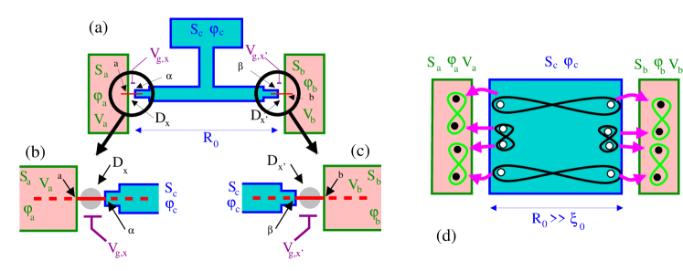
Specifically, we consider a -dot--dot- three-terminal Josephson junction made with the BCS superconductors , and and two quantum dots (see figures 1a, 1b and 1c). This physical system has the following features: (i) The time-periodic Floquet-Josephson dynamics with single characteristic frequency if biasing is at commensurate voltages Freyn ; Melin1 ; Jonckheere ; FWS ; Sotto ; engineering ; papierI ; papierII ; Josephson-dc ; (ii) The nonlocal electron-hole or hole-electron conversions, i.e. Cooper pair splitting exp-CPBS1 ; exp-CPBS2 ; exp-CPBS3 ; exp-CPBS4 ; exp-CPBS5 ; exp-CPBS6 ; exp-CPBS7 ; exp-CPBS8 ; theory-CPBS1 ; theory-CPBS2 ; theory-CPBS3 ; theory-CPBS4 ; theory-CPBS4-bis ; theory-CPBS4-ter ; theory-CPBS5 ; theory-CPBS6 ; theory-CPBS7 ; theory-CPBS8 ; theory-CPBS9 ; theory-CPBS10 ; theory-CPBS11 ; theory-noise8 ; theory-noise9 ; theory-noise11 ; (iii) The long-range quasiparticle propagation above the gap between the two remote quantum dots separated by the distance . Then, we demonstrate that (i), (ii) and (iii) automatically imply large-scale quantum-mechanical clusters of Cooper pairs between the constituting -dot- junctions, even if the distance between them is much larger than the zero-energy superconducting coherence length , i.e. if . These clusters can be viewed as being “the elementary quantum particles” that are exchanged between the two Floquet-Josephson junctions in a three-terminal configuration. Figure 1d features real-space representation of the lowest-order four-Cooper pair cluster corresponding to the “ultralong-distance Floquet-Tomasch octets”.
In the absence of bias voltage, all superconducting leads are grounded and the three-terminal -- Josephson junction Freyn ; Pillet ; Pillet2 ; Scherubl ; Nazarov-PRR ; Nazarov-PRB-AM can be phase-biased with appropriate superconducting loops. The Andreev bound states Andreev ; Bretheau1 ; Bretheau2 ; Schindele ; Olivares ; Janvier ; Gramich1 ; Bretheau3 ; Gramich2 ; Dassonneville ; Tosi are then coupled by the overlapping evanescent Bogoliubov-de Gennes wave-functions at a double interface, forming “Andreev molecules” with avoided crossings in their spectra, see Refs. Pillet, ; Pillet2, . At equilibrium, nonlocality is limited by the superconducting coherence length as a function of the distance between the - and - interfaces Pillet ; Pillet2 ; Scherubl ; Nazarov-PRR ; Nazarov-PRB-AM .
We note that a DC-Josephson-like resonance appears if the three superconducting terminals are biased on the “quartet line” Freyn :
| (1) |
The resulting Josephson relations , and for the superconducting phase variables at time imply the static “quartet phase variable” Freyn . This yields the quartet current-phase relation in the limit of low values of the contact transparencies. The three recent experiments of the Grenoble Lefloch , Weizmann Institute Heiblum and Harvard Kim groups show all signs of compatibility with the theory of the quartets Freyn ; Melin1 ; Jonckheere ; Sotto ; FWS ; engineering ; papierI ; papierII , in addition to other experiments multiterminal-exp1 ; multiterminal-exp2 ; multiterminal-exp3 ; multiterminal-exp4 ; multiterminal-exp5 ; multiterminal-exp6 ; multiterminal-exp7 on multiterminal Josephson junctions. The reason why some experiments report the quartets while others do not is maybe a complex matter of the materials and geometry.
The present paper focuses on the range of the quartets at finite bias voltage being a fraction of the superconducting gap . Concerning propagation across between the two Josephson junctions, the Tomasch effect was experimentally shown in Refs. Tomasch1, ; Tomasch2, ; Tomasch3, to produce oscillations in the density of states of the superconducting quasiparticles in a two-terminal configuration, as a result of the finite superconducting film thickness reaching m in the experimental Ref. Tomasch3, . The “Tomasch effect” Tomasch1 ; Tomasch2 ; Tomasch3 and the model proposed by McMillan and Anderson McMillan-Anderson provide sensitivity on the thin film boundary conditions, corresponding to the two-terminal nonlocal density-phase response, see also the contribution of Wolfram and Lehman Wolfram . The here considered three-terminal “Floquet-Tomasch effect for the Cooper pair clusters” couples one junction to the phase drop at the other junction according to the nonlocal current-phase response and it does not involve the same microscopic quantum process as the three-terminal density of state oscillations. The former is DC-current current response and the latter corresponds to AC-density oscillations. Nonlocality and quantum correlations are obtained in the Floquet-Tomasch effect over the ultralong-distance that is orders of magnitude larger than at equilibrium.
This ultralong-distance effect contrasts with the ferromagnet-superconductor-ferromagnet and the normal metal-superconductor-normal metal beam splitters, where nonlocality and quantum correlations are limited by the superconducting coherence length , see for instance Refs. exp-CPBS1, ; exp-CPBS2, ; exp-CPBS3, ; exp-CPBS4, ; exp-CPBS5, ; exp-CPBS6, ; exp-CPBS7, ; exp-CPBS8, ; theory-CPBS1, ; theory-CPBS2, ; theory-CPBS3, ; theory-CPBS4, ; theory-CPBS4-bis, ; theory-CPBS4-ter, ; theory-CPBS5, ; theory-CPBS6, ; theory-CPBS7, ; theory-CPBS8, ; theory-CPBS9, ; theory-CPBS10, ; theory-CPBS11, ; theory-noise8, ; theory-noise9, ; theory-noise11, .

The paper is organized as follows. The physical picture is presented in section II. The model and methods are presented in section III. Analytical model calculations are presented in section IV. Section V deals with presentation of the numerical results. Perspectives on noise measurements are discussed in section VI. Summary of the paper is provided in section VII.
II Physical picture
We first present the basics of Cooper pair splitting and nonlocality limited by the superconducting coherence length, see Refs. exp-CPBS1, ; exp-CPBS2, ; exp-CPBS3, ; exp-CPBS4, ; exp-CPBS5, ; exp-CPBS6, ; exp-CPBS7, ; exp-CPBS8, ; theory-CPBS1, ; theory-CPBS2, ; theory-CPBS3, ; theory-CPBS4, ; theory-CPBS4-bis, ; theory-CPBS4-ter, ; theory-CPBS5, ; theory-CPBS6, ; theory-CPBS7, ; theory-CPBS8, ; theory-CPBS9, ; theory-CPBS10, ; theory-CPBS11, ; theory-noise8, ; theory-noise9, ; theory-noise11, . The range of Cooper pair splitting is introduced in section II.1 for three-terminal and devices. Next, we proceed further in section II.2 with the ultralong-distance Floquet-Tomasch effect in a three-terminal ---- Josephson junction, where and denote the two quantum dots.
II.1 Nonlocality of Cooper pair splitting
This subsection introduces nonlocality and quantum correlations in a three-terminal or device, in connection with Cooper pair splitting, see Refs. exp-CPBS1, ; exp-CPBS2, ; exp-CPBS3, ; exp-CPBS4, ; exp-CPBS5, ; exp-CPBS6, ; exp-CPBS7, ; exp-CPBS8, ; theory-CPBS1, ; theory-CPBS2, ; theory-CPBS3, ; theory-CPBS4, ; theory-CPBS4-bis, ; theory-CPBS4-ter, ; theory-CPBS5, ; theory-CPBS6, ; theory-CPBS7, ; theory-CPBS8, ; theory-CPBS9, ; theory-CPBS10, ; theory-CPBS11, ; theory-noise8, ; theory-noise9, ; theory-noise11, .
Andreev reflection Andreev at a normal metal-superconductor () interface converts the supercurrent carried by Cooper pairs in into normal current in . Namely, spin-up electron from is Andreev-reflected as a spin-down hole and a Cooper pair is transmitted into the condensate. The semiclassical trajectories of the incoming electron and outgoing hole are separated on the interface by less than the superconducting coherence length , which is why Andreev reflection is nonlocal at the scale of the superconducting coherence length.
The experimental evidence exp-CPBS1 ; exp-CPBS2 ; exp-CPBS3 ; exp-CPBS4 ; exp-CPBS5 ; exp-CPBS6 ; exp-CPBS7 ; exp-CPBS8 for the theoretical prediction of nonlocal Andreev reflection theory-CPBS1 ; theory-CPBS2 ; theory-CPBS3 ; theory-CPBS4 ; theory-CPBS4-bis ; theory-CPBS4-ter ; theory-CPBS5 ; theory-CPBS6 ; theory-CPBS7 ; theory-CPBS8 ; theory-CPBS9 ; theory-CPBS10 ; theory-CPBS11 ; theory-noise8 ; theory-noise9 ; theory-noise11 involves three-terminal configurations, such as the above mentioned or devices.
Regarding the range of Cooper pair splitting in three-terminal and devices, the zero-energy superconducting coherence length is given by
| (2) |
in the ballistic limit, where is the Fermi velocity. This “size of a Cooper pair” is energy/frequency--sensitive:
| (3) |
where is the Fermi velocity. Eq. (3) diverges as the energy goes to the superconducting gap , see also Ref. Madrid, for the nonlocal conductance at arbitrary bias voltage with respect to the superconducting gap.
II.2 Ultralong-distance Floquet-Tomasch effect
The introduction of “the Feynman diagrams” in calculations of the light-matter interaction was not only useful to represent the quantum processes, but it also yielded considerable shortcuts in the calculation of those scattering amplitudes. Here, the diagrams yield intuitive explanations and simple physical pictures for the numerical results presented in section V. Those diagrams represent the time-evolution of the electrons, holes and the conversions between them, scattering back and forth between the different interfaces.
This subsection considers nonlocality in the ---- three-terminal Josephson junction on figures 1a, 1b and 1c which is biased according to Eq. (1) in a voltage- range that is significant fraction of the superconducting gap , typically . Specifically, we detail the microscopic processes, starting with the nonlocal pair amplitude, and next proceeding further with the Floquet-Andreev and the Floquet-Tomasch contributions to the current, finally uncovering the ultralong-distance Floquet-Tomasch octets. We demonstrate in Appendix A that the Floquet-Tomasch effect for the current of pairs in a three-terminal Josephson junction and the two-terminal density of state oscillations in the Tomasch effect Tomasch1 ; Tomasch2 ; Tomasch3 ; McMillan-Anderson ; Wolfram share the ultralong-distance nonlocality, but the corresponding quantum processes are inequivalent. Thus, the mechanism for the two-terminal density of state oscillations in the Tomasch effect Tomasch1 ; Tomasch2 ; Tomasch3 ; McMillan-Anderson ; Wolfram cannot be advocated to be at the origin of the ultralong-distance current of pairs in the three-terminal Josephson junction. In the first place, in the three-terminal configuration, the quantum processes coupling the density of states at one contact to the pairs at the other contacts are AC at the lowest-order in the tunneling amplitudes, and thus, they cannot be put forward as an explanation to the calculated three-terminal DC-current of quartets and higher-order clusters of Cooper pairs.
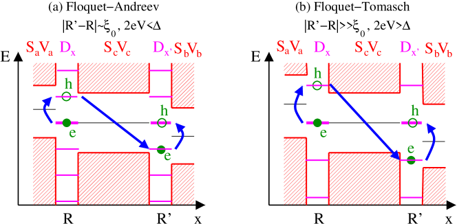
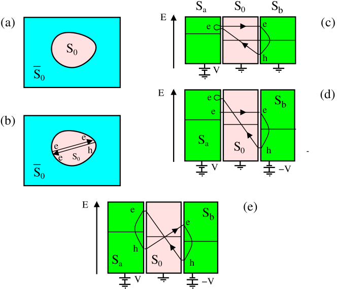
Figures 2a and 2b show the energy diagram for the lowest-order pair amplitude between the quantum dots and , corresponding to conversion of “spin-up electron on the dot ” into “spin-down hole on the dot ”.
The processes on figures 2a and 2b start with electron-hole conversion at the -- Josephson junction: local Floquet-Andreev reflection first increases the energy by (i.e. the energy of a Cooper pair taken from the lead biased at the voltage ). The process continues with nonlocal propagation from to across in the hole-electron channel. Next, “local” inverse-Floquet hole-electron conversion takes place at the -- Josephson junction. In the final state, spin-down hole is produced at zero energy on the quantum dot .
The condition on the bias voltage (see figure 2a) implies conversion in the hole-electron channel over the superconducting coherence length , see Eq. (3). This subgap process is referred to as “the Floquet-Andreev quartet pair amplitude”.
Conversely, on figure 2b implies nonlocal hole-electron conversion above the gap of . This process is limited by the mesoscopic phase coherence length of the superconducting quasiparticles, and it is referred to as “the ultralong-distance Floquet-Tomasch pair amplitude” [see the forthcoming Eqs. (11)-(18)], in analogy with the Tomasch effect Tomasch1 ; Tomasch2 ; Tomasch3 ; McMillan-Anderson mentioned above in the Introduction.
Emergence of the ultralong-distance Floquet-Tomasch pair amplitude if implies ultralong-distance nonlocality over , and quantum correlations in the -sensitive current, which is considered now.
Now, we “close the loop” on figures 3a and 3b with final zero-energy hole-electron conversion from to . The resulting -sensitive Floquet-Andreev quartet current is limited by the superconducting coherence length , independently on whether or .
Finally, we consider the higher-order process of the ultralong-distance Floquet-Tomasch octets having -sensitivity and range limited by . Figure 4 shows the corresponding diagram, see also figure 1d. Two nonlocal and two local hole-electron conversions are involved: (i) Nonlocally from to and from to across , and (ii) Locally between each and , the and quantum dots and . Overall, the resulting -sensitive octet current appears if the distance between the remote -- and -- junctions reaches , such that . We conclude that figure 4 provides microscopic picture for the proposed ultralong-distance Floquet-Tomasch octets as an eight-fermion cluster originating from four Cooper pairs, see also figure 1d.
This physical picture suggests cross-over as increases from below to above , i.e. from “the dominant of the Floquet-Andreev quartets over ” to “the dominant of the ultralong-distance Floquet-Tomasch octets over ”. A cross-over to the higher-order- clusters of Cooper pairs is expected as the voltage values is reduced below (with an integer).
We proceed further with the models and methods in section III, next with the analytical results in section IV and finally the theory is put to the test of the numerical calculations in section V.
III Model and methods
We start in subsection III.1 with a brief description of the models used in the paper, i.e. the geometry and the Hamiltonians. Next, we present in subsection III.2 a central ingredient of the model, i.e. the connection between the Dynes parameter and the mesoscopic phase coherence length of the superconducting quasiparticles. The methods are mentioned in section III.3.
III.1 Geometry and Hamiltonians
Now, we present the geometry and the Hamiltonians.
Figures 1a, 1b and 1c show the device geometry: the T-shaped grounded superconducting lead connected via the two quantum dots and to and biased at . Those figures represent quasi-one-dimensional semiconducting nanowire quantum dots similar to Ref. Heiblum, . The distance between and is denoted by .
Now, we provide the Hamiltonians. The BCS Hamiltonian of each infinite superconducting lead with gap and phase is given by
| (4) | |||||
| (5) |
where, again, is the projection of the spin along the quantization axis, and takes the values , or according to which of the superconducting lead , or is considered. The notation in Eq. (4) stands for pairs of neighboring sites on a three-dimensional (3D) tight-binding lattice, and the label in Eq. (5) runs over all tight-binding sites.
The tunnel Hamiltonian couples the tight-binding sites on both sides of the contacts:
| (6) |
where in Eq. (6) denotes the pairs of corresponding tight-binding sites on both sides of the two-dimensional (2D) interface.
The Hamiltonian of a direct-gap semiconductor making the quantum dots on figure 5 is inspired by Ref. Gavoret, . We take the following Hamiltonian in the infinite 3D bulk limit:
| (7) |
where or create spin- fermions with the wave-vector in the conduction or valence band, and is the value of the direct gap. We will use in section IV the fact that the dispersion relations appearing in Eq. (7) have extrema at the wave-vector .
Considering the pair of tight-binding sites making the contact at the interface between the superconductor and the quantum dot (see figure 5), the local creation operator on the surface is defined as a sum over the quantum numbers and of the and creation operators associated to both conduction and valence band respectively:
| (8) |
where we assumed a quantum dot with finite dimension, and the tight-binding site labeled by is at the space coordinate . In Eq. (8), the quantum numbers and label the states of the quantum dot with finite dimension, possibly with irregularities in its shape, and having Eq. (7) as its bulk Hamiltonian. The notations and stand for the corresponding conduction and valence band wave-functions.
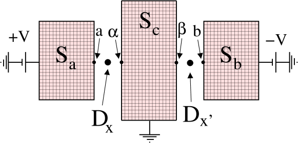
The zero-dimensional (0D) quantum dot on figure 6 has level at zero energy. Thus, the corresponding Hamiltonian is .
The quantum dots are connected with highly transparent interfaces to the leads, which is why the Coulomb interaction is included neither in Eq. (7) nor in . For instance, the recent experiments multiterminal-exp7 on Andreev molecules Pillet ; Pillet2 ; Scherubl ; Nazarov-PRR ; Nazarov-PRB-AM do not seem to require Coulomb interactions as a central ingredient, because of the highly transparent interfaces.
Zero temperature is assumed throughout the paper. Nontrivial quasiparticle populations can be produced at zero temperature by driving normal current between two attached normal leads. An interesting theoretical and experimental question is to address whether driving normal current can result in change of sign of the quartet critical current, similarly to two terminals, see Refs. vanWees-PRB, ; vanWees, .
The scattering approach or the Keldysh Green’s functions Caroli were complementary used in the past to address superconducting junctions, see for instance Refs. Averin, ; Cuevas, ; Cuevas-noise, for a single superconducting weak link. Both approaches have their own advantages. For instance, the scattering matrix calculations and the wave-function approach allow for semiclassical calculations, see Refs. Berry, ; Bratus, . Microscopic Green’s functions produce efficient algorithms to address the general conditions of high transparencies and large current bias, see for instance Ref. Madrid, . In the following, we rely on the Keldysh Green’s functions, on the basis of the algorithms that were developed over the last few years FWS ; Sotto ; engineering ; papierII ; Berry .
We also implement the simplifying assumption of a ballistic superconductor, similarly to the McMillan-Anderson and the Wolfram-Lehman papers McMillan-Anderson ; Wolfram on the Tomasch effect Tomasch1 ; Tomasch2 ; Tomasch3 . Taking the ballistic limit yields considerable simplifications in the calculations, see below. Disorder in the superconductors could be introduced in the future on the basis of the Usadel equations Usadel . Another possible approach is to assume perturbation theory in the strength of the nonlocal processes between the two quantum dots, see the forthcoming section IV, and to average over disorder the pairs of nonlocal Green’s functions connecting both quantum dots. The Nambu components of the advanced-advanced transmission modes (see Ref. papierI, ) would then have to be generalized to the Keldysh contour and to energy outside the superconducting gap.
III.2 The mesoscopic phase coherence length of the superconducting quasiparticles
In this subsection, we relate the mesoscopic phase coherence length of the superconducting quasiparticles to the Dynes parameter FWS ; Kaplan ; Dynes ; Pekola1 ; Pekola2 .
By the time-energy uncertainty relation, and by the correspondence between the time and length scales, a characteristic length is associated to any energy scale . To the Fermi energy is associated the Fermi wave-length , which is much smaller than the superconducting coherence length that is related to the superconducting gap . The characteristic length is conjugate to the Dynes parameter , and it phenomenologically accounts for the quantum-to-classical cross-over of the propagating superconducting quasiparticles, due to inelastic scattering and energy relaxation. Then, is much larger than the superconducting coherence length , i.e. , because the Dynes parameter is much smaller than the superconducting gap , i.e. , see Refs. FWS, ; Kaplan, ; Dynes, ; Pekola1, ; Pekola2, . The length scale has to cross-over to its normal-state value as the energy crosses-over above . This naturally receives the interpretation of defining the “limit of the quantum world” as far as the superconducting quasiparticle propagation is concerned.
Now, within this phenomenological “Dynes picture”, we provide analytical expressions for the mesoscopic phase coherence length of the superconducting quasiparticles as a function of the energy .
The evanescent Bogoliubov-de Gennes wave-functions decay exponentially like from the interface at the subgap energy , see also the Green’s function given by Eq. (58). Then, the superconducting coherence length can be continued to energies outside the gap, and it has the following real and imaginary parts:
which yields damping and oscillations:
| (10) |
We define the inverse damping length as
| (11) |
with .
We note that , where . Using leads to
Assuming and yields
| (13) | |||
and
| (14) | |||
where we used if . The following is deduced:
| (15) |
and is given by
| (16) |
Then, if the energy takes the typical value :
| (17) |
This yields
| (18) |
where is expressed in units of the zero-energy superconducting coherence length , see Eq. (2). The Dynes ratio is small in the experiments Kaplan ; Dynes ; Pekola1 ; Pekola2 , which implies the ultralong-distance effect corresponding to in Eq. (18).
Thus, Eq. (18) supports the idea presented in the Introduction, i.e. within this Dynes picture, the mesoscopic phase coherence length of the superconducting quasiparticles is orders of magnitude larger than the zero-energy superconducting coherence length in a typical energy window that can roughly be estimated as . This typical spectral window for emergence of the ultralong-distance Floquet-Tomasch effect reflects the coexistence of both features of the normal and superconducting states, i.e. long and sizeable nonlocal Andreev processes.
Controlling the electromagnetic environment as in Ref. Pekola1, can reduce the value of the Dynes parameter by orders of magnitude, and produce large value of according to Eqs. (11)-(18). This can also be used to rule out the coupling to the electromagnetic environment as the origin of the quartet line. In the previous Grenoble Lefloch and Weizmann group experiments Heiblum , a device fabricated with remote junctions did not produce the quartet line in spite of the same electromagnetic environment as in the device with close junctions.
III.3 Methods
IV Analytical results
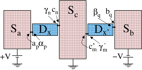
In this section, we assume that the quantum dots are fabricated with direct-gap semiconductors [see Eq. (7)], and we map “the model I” on figure 5 onto “the reduced model II” on figure 6. We also provide analytical results demonstrating the Floquet-Andreev quartets and the ultralong-distance Floquet-Tomasch octets, discuss the absence of dephasing in propagation between the two interface and explain why the ultralong-distance effect appears both for the two-terminal density of states in the Tomasch experiments Tomasch1 ; Tomasch2 ; Tomasch3 , and for the pair current in the here considered three-terminal Josephson junction. However, the quantum processes are distinct from each other and it turns out that the nonlocal coupling between the density of states at one contact and the pairs at the other contact is AC in the three-terminal Josephson junction.
Specifically, starting with the model I in figure 5, we assume that the Nambu Green’s function of each quantum dot or fulfills the following “generalized star-triangle relation”, i.e. we propose the following for the quantum dot :
| (19) | |||||
| (20) |
The assumption of resonance at zero energy implies , see the discussion following Eq. (56) in Appendix B. We consider that the quantum dots have minimum at the wave-vector in their dispersion relation, see Eq. (7). We assume that the contact dimension is small compared to and that the size of the quantum dots is small compared to the decay length of the evanescent wave-functions on the dot. Then, and are roughly independent on and is the matrix square root of the residue in Eq. (57).
The Green’s functions are matrices in Nambu and in the enlarged space of the harmonics of the Josephson frequency. The labels running over the tight-binding sites at the interfaces are now made implicit [see Eqs. (19)-(20)].
The fully dressed Green’s function on the dot can be “expanded in nonlocality” according to
| (21) | |||||
| (22) | |||||
| (23) | |||||
| (24) |
where and describe “local” dressing at the -- and -- junctions, and the matrices and correspond to nonlocal propagation from to and from to respectively, see Appendix C. An expansion similar to Eqs. (21)-(24) was previously developed for the nonlocal conductance of or beam splitters, see Ref. theory-CPBS11, . Here, the small parameter for nonlocality of the Floquet-Andreev quartets is , due to transmission of quasiparticles via evanescent states in the subgap energy window. The small parameter for the Floquet-Tomasch octets is instead of the previous , corresponding to propagation via plane waves in a spectral window above the gap of , and damping over the mesoscopic phase coherence length , see Eqs. (11)-(16).
The first term in Eq. (21) does not couple the two quantum dots. The Keldysh component of the second term in Eq. (22) is the following:
| (25) |
Specifying the Nambu labels corresponding to anomalous propagation between and leads to
| (26) |
Within this approximation, the Floquet-Tomasch quartets and octets propagate a pair of nonlocal Green’s functions between the two quantum dots, where Eq. (26) also captures “local” dressing by multiple Andreev reflections at each -dot- Josephson junction.
The Floquet-Andreev quartets correspond to
where the “” labels are used for the Nambu and Floquet labels respectively. Both and entering Eq. (IV) are of order if , due to the corresponding dominant contribution of the subgap energy window. Thus, in Eq. (26) is of order .
The Floquet-Tomasch Keldysh Green’s function is given by
where and entering Eq. (IV) are both of order if . Thus, in Eq. (IV) is of order .
Eqs. (IV)-(IV) imply that the current on the quartet line is expressed as summation over and at the - and - interfaces respectively, see figure 5: . Then, Eq. (64) in Appendix B yields
| (29) |
Gathering the Green’s functions in a pair-wise manner HN1 ; HN2 yields and
| (30) |
where is the spectral current of the “reduced model II on figure 6” at the distance between the 0D quantum dots.
Thus, the use of direct-gap semiconductor quantum dots allows replacing “the multichannel contacts of the model I ” by “the 0D quantum dots of the reduced model II” while averaging over in Eq. (64). We also singled-out the Floquet-Andreev quartet and the ultralong-distance Floquet-Tomasch octet contributions to the current, which supports the physical picture of the preceding sections II and III, and the numerical results of the forthcoming section V.
We also note that biasing at produces coinciding gap edge singularities of and . This is expected to result in large values for the quartet and octet critical currents and , as for perfectly transparent contacts. The following scaling form of and at the voltages can be conjectured:
| (31) | |||||
| (32) |
Both and are expected to be reduced if the bias voltage is detuned from . This Eq. (32) will further be considered in the next section on the numerical data.

Finally, we underline consistency with Ref. McMillan-Anderson, regarding robustness with respect to dephasing between the corresponding pairs of Green’s function. The superconducting Green’s function in Eq. (64) is rewritten as
| (34) | |||||
where
| (38) | |||||
| (41) |
and is the distance between and . We assume that the Fermi wave-length is much smaller than all other length scales:
| (42) | |||
| (43) |
In addition, the characteristic dimension of the quantum dot is such that , which implies that the oscillations are not washed-out by extended contacts. Then, using the notation
| (44) |
for averaging over in the interval , see Eq. (30), we express the averaging of the pairs of Nambu Green’s functions as follows:
The corresponding anomalous components involve one or two nonlocal Andreev electron-hole or hole-electron conversion. They take sizeable values if , are typically in the energy window instead of being strictly inside the gap according to . This implies that the ultralong-distance effect holds for all of the quantum electron-hole conversion processes captured by Eq. (IV), and being characterized by different sets of the corresponding 16 Nambu labels. As a consequence, both the density of state oscillations of the two-terminal Tomasch effect and the clusters of Cooper pairs in the three-terminal Josephson junction are characterized by the corresponding ultralong-distance coupling, see also Appendix A where the demonstration starts from the different point of view of the open boundary conditions considered by Wolfram and Lehman in Ref. Wolfram, . However, it is also shown in this Appendix A that the coupling between the density of states at one contact and the pairs at the other contact is AC in the three-terminal Josephson junction. Thus, those AC density of state oscillations in a three-terminal Josephson junction cannot explain the following numerical data on the DC-current of clusters of Cooper pairs also with three superconducting terminals.
To interpret the finite electron-hole or hole-electron conversion amplitude above the gap, in a characteristic spectral window , we refer to Fig. 7a in the Blonder-Tinkham-Klapwijk approach BTK , showing the sizeable Andreev reflection conductance of a highly-transparent normal metal-superconductor junction as a function of voltage such that .
In addition, the quasiparticles and pairs in the Tomasch oscillations in the two-terminal density of states Tomasch1 ; Tomasch2 ; Tomasch3 copropagate over ultralong-distance, and they can be referred to as “the triplets correlations” triplet between a single quasiparticle and a pair. Conversely, two copropagating pairs correspond to “the so-called quartets” in three-terminal Josephson junctions Freyn . A possibility is to speculate that enhanced condensation energy could be produced by those propagating Nambu modes acting like a “glue”, in addition to the mean field BCS pairing. Indeed, it would be interesting to consider analogies with the theory of the collective modes collective1 ; collective2 ; collective3 , and to examine whether those “triplets” or “quartets” can possibly give rise to a collective state upon taking the Coulomb interaction or strong disorder into account.
V Numerical results
In this section, we provide selection of numerical data for the reduced model II, defined in the above section IV.
We successively introduce the calculations and present the ultralong-distance effect, see figures 7 and 8. Next, we present the cross-over from the Floquet-Andreev quartets to the ultralong-distance Floquet-Tomasch octets in the quartet phase sensitivity of the current, as the distance between the dots is increased from to and to , see figures 9 and 10.
The current of the ---- double quantum dot three-terminal Josephson junction is obtained from the fully dressed Dyson-Keldysh equations to all orders in the tunneling amplitudes. Concerning the algorithms, the code is based on numerically exact implementation of the Dyson and Dyson-Keldysh Eqs. (71)-(72), see Appendix B. The Dyson Eq. (71) is solved with recursive Green’s functions in energy Cuevas and sparse matrix algorithms are used for the matrix products. Details about the algorithms can be found in the Appendix of Ref. Sotto, .
Based on symmetry arguments Melin1 ; Jonckheere , we implement the hopping amplitudes and , thus with and for the normal-state line-width broadening parameters . Then, we evaluate the current of the clusters of Cooper pairs as
where the currents and are transmitted into and , and in Eq. (V) is averaged over according to Eq. (30).
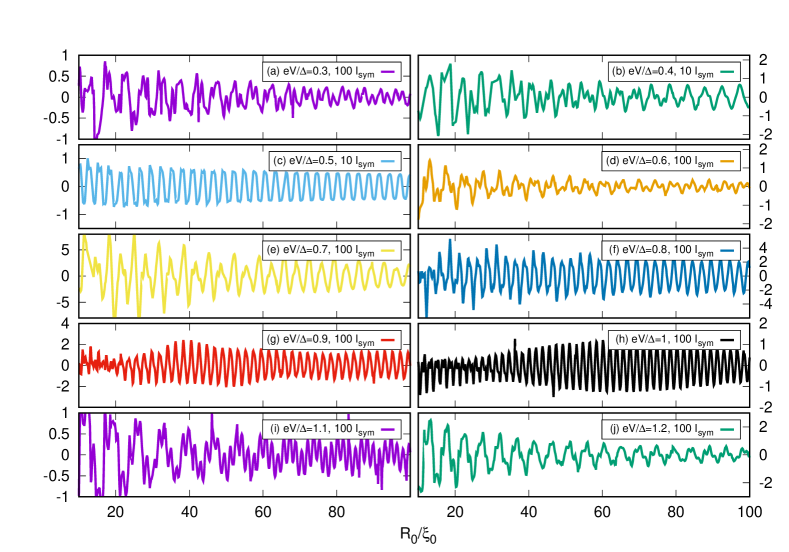
We start with the sensitivity of on the distance between the quantum dots and . The data on figure 7 show the current as a function of at the fixed quartet phase and for the reduced voltage values from to on panels a-j respectively. The numerical data on figure 7 feature complex pattern of the Floquet-Tomasch oscillations. The beatings are interpreted as interference between the wave-vectors of the quantum dot level Floquet replica. The numerical data on figure 7 fully confirm the physical picture of section II regarding the ultralong-distance Floquet-Tomasch oscillations. The value of the Dynes parameter used in figure 7 implies , see Eqs. (11)-(16). This is compatible with emergence of sizeable at on figure 7. By contrast, is limited by in the recently considered Andreev molecules with all superconducting leads grounded Freyn ; Pillet ; Pillet2 ; Scherubl ; Nazarov-PRR ; Nazarov-PRB-AM , and in the and Cooper pair beam splitters, see Refs. exp-CPBS1, ; exp-CPBS2, ; exp-CPBS3, ; exp-CPBS4, ; exp-CPBS5, ; exp-CPBS6, ; exp-CPBS7, ; exp-CPBS8, ; theory-CPBS1, ; theory-CPBS2, ; theory-CPBS3, ; theory-CPBS4, ; theory-CPBS4-bis, ; theory-CPBS4-ter, ; theory-CPBS5, ; theory-CPBS6, ; theory-CPBS7, ; theory-CPBS8, ; theory-CPBS9, ; theory-CPBS10, ; theory-CPBS11, ; theory-noise8, ; theory-noise9, ; theory-noise11, . We also note that, strictly speaking, given by Eq. (2) and given by Eq. (17) are two independent length scales, in the sense that is not proportional to . The current was averaged over the oscillations at the scale of the Fermi wave-length according to Eq. (30). Then, is the smallest length-scale to which the calculated couples and it is illustrative to plot as a function of .
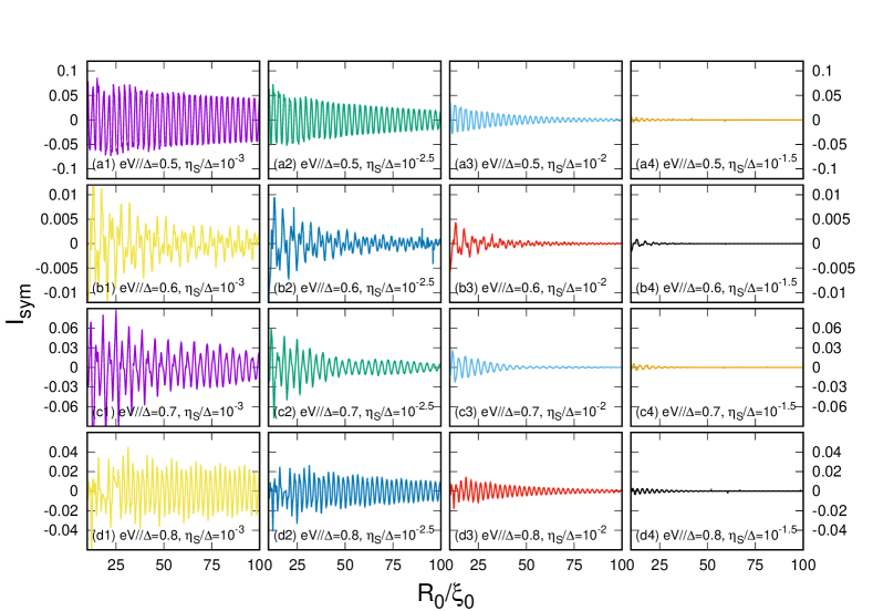
Figure 8 illustrates the effect of the Dynes parameter on the current . On this figure, the Dynes parameter ranges from (on panels a1, b1, c1, d1) to (on panels a2, b2, c2, d2), (on panels a3, b3, c3, 3) and (on panels a4, b4, c4, d4). The voltage values are on panels a1-a4, b1-b4, c1-c4 and d1-d4 respectively. It is concluded that the range of the Floquet-Tomasch effect is strongly reduced by increasing the Dynes parameter from to , in agreement with the physical arguments presented in the preceding sections II, III and IV.
We also deduce from the -scales on figure 7 that the current reaches maximum around , i.e. for on figures 7b and 7c is one order of magnitude larger than for on figures 7a and 7d. The strong enhancement of at is interpreted as the coinciding upper and lower gap edge singularities of and which are biased at , as if the contact transparencies would be enhanced by orders of magnitude in this voltage window, see the remarks related to Eqs. (31)-(32) in the previous section IV.
It is also visible on figures 8 and 9 that the current is larger for than for . The voltage-dependence of is indeed expected to be nonmonotonic, because of the interplay between the voltage- sensitive peaks in the density of states coming from the quantum dot Floquet replica, and the BCS gap edge singularities, see the diagrams on figure 4.
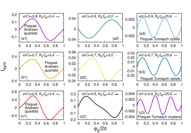
The cross-over from the Andreev quartets to the ultralong-distance Floquet-Tomasch octets was proposed in section II as is increased from to and next to . Figures 9 and 10 show how depends on the quartet phase at fixed values of the reduced voltage and distance between the quantum dots. The values and are used on figure 9, and are used on figure 10.
In general, the symmetric current has dominant quartet, octet or higher-order -sensitivity, namely , or respectively.
The voltage on figures 9-a1, 9-a2 and 9-a3 confirms the cross-over from the Andreev quartets to the ultralong-distance Floquet-Tomasch octets as is increased from to and to . The dominant and are obtained for the small and for the intermediate on figures 9-a1 and 9-a2, while the dominant of the ultralong-distance Floquet-Tomasch octets is obtained for on figure 9-a3.
We also proposed in section II emergence of higher-order harmonics in the current-quartet phase relation as is reduced. To illustrate this point, we now reduce the bias voltage to (see figures 9-b1, 9-b2 and 9b3) and to (see figures 9-c1, 9-c2 and 9-c3). The following voltage values are also used on figure 10: (see figures 10-a1, 10-a2, 10-a3), (see figures 10-b1, 10-b2, 10-b3) and (see figures 10-c1, 10-c2, 10-c3). The dominant harmonics emerges for on figure 9-c3, and for , on figures 10-a3 and 10-b3. The higher-order harmonics is also obtained for on figure 10-c3.
We note consistency with our previous results for a single 0D quantum dot Sotto . Namely, and on figures 9-a1, 9-a2 and 9-c1 and on figures 10-a1, 10-a2 and 10-c1 feature the -to- and -to- cross-overs which were found in our previous Ref. Sotto,
To summarize, the numerical calculations confirm the physical picture of section II, Appendix A and the analytical results of section IV regarding the following items: (i) The ultralong range of the effect and the way it depends on the Dynes parameter ratio , (ii) The sensitivity on the quartet phase , i.e. the cross-over from the Andreev quartets to the ultralong-distance Floquet-Tomasch octets as is increased from to and to , (iii) The voltage dependence of the effect, i.e. the emergence of higher-order harmonics at smaller values of the voltage , and (iv) The emergence of large ultralong-distance signal if , which becomes weaker if is tuned away from .
VI Discussion
In this section, we discuss consequences for probing the “quantumness” of the Floquet-Tomasch clusters of Cooper pairs with quantum current-noise cross-correlations. We distinguish between theory (see subsection VI.1) and possible experiments (see section VI.2).
VI.1 Quantum current-noise cross-correlations
The price to pay for nonlocal clusters of Cooper pairs over the ultralong-distance is apparently to renounce to a “good Floquet qu-bit”. Considering that the bias voltage energy is much smaller than the superconducting gap , the Floquet resonance line-width broadening is limited by multiple Andreev reflections FWS ; papierII ; engineering ; Berry , at least in the absence of “extrinsic” mechanism of relaxation FWS . We previously reportedFWS ; papierII ; engineering ; Berry that with of order unity, i.e. the line-width broadening is exponentially small as is reduced. But here, the coupling to the continua of quasiparticles above the gap produces significant broadening of the Floquet resonances and small coherence time FWS ; papierII ; engineering ; Berry at higher voltage values, from to on figures 7, 8 and 9.
This “poor Floquet qu-bit” does however not preclude emergence of quantum correlations at the ultralong distance , because the Cooper pair clusters are composite objects made of both the “locally transmitted” and “nonlocally split” Cooper pairs, see figure 1d. It is known that, in general, breaking Cooper pairs produces quantum mechanical correlations and entanglement, see the and the beam splitters theory-CPBS3 ; theory-CPBS4 ; theory-CPBS4-bis ; theory-CPBS4-ter ; theory-CPBS5 ; theory-CPBS6 ; theory-CPBS7 ; theory-CPBS8 ; theory-CPBS9 ; theory-CPBS10 ; theory-CPBS11 ; theory-noise8 ; theory-noise9 ; theory-noise11 . Nonvanishingly small zero-frequency quantum current-noise cross-correlations in a -dot--dot- three-terminal Josephson junction at the ultralong is a possibility for experimental demonstration of the quantum nature of the ultralong-distance Cooper pair clusters.
In fact, the quantum current-noise cross-correlation kernel
| (47) |
was calculated by many authors, see for instance Ref. Cuevas-noise, and Eqs. (15)-(19) in our preceding Ref. Sotto, :
| (48) | |||||
| (49) | |||||
| (50) | |||||
| (52) | |||||
where is a Pauli matrix, are the time variables and we assume -- three-terminal device which is connected at the tight-binding sites -- with the hopping amplitudes and . Eqs. (48)-(52) can be Fourier transformed from the time variables to the energies and , where and are two integers.
The nonvanishingly small current of the quartets, octets or higher-order clusters of Cooper pairs at the ultralong implies nonvanishingly small Keldysh Green’s functions and , see the corresponding expressions of the current in Eq. (V), Eq. (73) and Eqs. (78)-(78). Then, at the ultralong emerges on the condition that and in Eqs. (48)-(52) take values in overlapping energy intervals, i.e. the bias voltage should also be nonvanishingly small. In practice, the bias voltage energy is a significant fraction of the superconducting gap .
Thus, within our model, the reported current implies quantum current-noise cross-correlations due to the quantum fluctuations of the current operators at the ultralong-distance . Possible quantum noise cross-correlation experiments are considered now.
VI.2 Proposed current cross-correlation experiments
On the experimental side, the positive zero-frequency quantum current-noise cross-correlations of the quartets were predicted Sotto and measured in the Weizmann group experiment Heiblum . In this experiment, absence of the quartet line and vanishingly small quantum current-noise cross-correlations were obtained with a pair of “remote” Josephson junctions. It was then concluded that “the trivial effect” of the electromagnetic environment is not at the origin of the quartet resonance line. The Grenoble experiment Lefloch also ruled out “extrinsic synchronization” by demonstrating absence of the quartet line with remote contacts in a metallic structure.
The bias voltage was very low with respect to the superconducting gap in the Weizmann group experimentHeiblum , i.e. . Here, we propose analogous measurement of the quantum current-noise cross-correlations at voltage values that are significant fractions of the gap; typically is within the same range as on figures 7, 8, 9 and 10, i.e. from to , given the above mentioned “gap edge singularity resonance” at . We propose to systematically vary the distance between the junctions, in comparison with the superconducting coherence length and the mesoscopic phase coherence length . It is expected that the ultralong-distance Floquet-Tomasch clusters of Cooper pairs are above detection threshold, given the large signal in Tomasch experiment Tomasch1 ; Tomasch2 ; Tomasch3 .
VII Conclusions
Summary of the paper and final remarks are presented now.
We provided evidence for ultralong-distance nonlocality and quantum correlations in -dot--dot- three-terminal Josephson junctions where the constituting -dot- and -dot- are biased at opposite voltage on the quartet line. We presented physical arguments in section II and Appendix A, regarding the diagrammatic interpretation of nonlocality. Analytical theory was proposed in sections III and IV. We reduced the direct-gap semiconducting quantum dots to zero dimension, and demonstrated emergence of the Floquet-Andreev and Floquet-Tomasch currents limited by the relevant length scales of the superconducting coherence length and the mesoscopic phase coherence length of the superconducting quasiparticles respectively. The numerical calculations presented in section V reveal that the ultralong-distance Floquet-Tomasch clusters of Cooper pairs emerge if the separation between the Josephson junctions exceeds the superconducting coherence length by orders of magnitude, i.e. if . This results from a phenomenological description relying on the observation that the Dynes parameter is much smaller than the gap , which implies that the corresponding mesoscopic phase coherence length of the superconducting quasiparticles is much larger than the superconducting coherence length . In addition, in agreement with the physical arguments of section II, the voltage values are significant fractions of the superconducting gap , typically for a cluster of order , where is an integer. The typical spectral window for the ultralong-distance effect is roughly estimated as . Namely, the ultralong-distance effect is obtained and nonlocal Andreev processes are still sizeable if is not large compared to the superconducting gap . In this spectral window, the superconducting quasiparticles behavior reflects both the normal- and the superconducting-state properties. The numerical data confirm the expectation that increasing from to and to yields cross-over from the to the -sensitivities of the Floquet-Andreev quartets and the ultralong-distance Floquet-Tomasch octets respectively. Reducing below produces higher-order- clusters of Cooper pairs and dominant harmonics in the current, where is an integer.
The Tomasch oscillations Tomasch3 were experimentally observed with superconducting film thickness as large as m. Thus, in analogy with the Tomasch experiment Tomasch3 , we conjecture emergence of the ultralong-distance Floquet-Tomasch clusters of Cooper pairs if the separation between the -dot- and the -dot- Josephson junctions is made as large as m.
This predicted ultralong-range of the Floquet-Tomasch effect is spectacularly orders of magnitude above the corresponding for overlapping Andreev bound states at Pillet ; Pillet2 ; Scherubl ; Nazarov-PRR ; Nazarov-PRB-AM or for or Cooper pair beam splitters, see Refs. exp-CPBS1, ; exp-CPBS2, ; exp-CPBS3, ; exp-CPBS4, ; exp-CPBS5, ; exp-CPBS6, ; exp-CPBS7, ; exp-CPBS8, ; theory-CPBS1, ; theory-CPBS2, ; theory-CPBS3, ; theory-CPBS4, ; theory-CPBS4-bis, ; theory-CPBS4-ter, ; theory-CPBS5, ; theory-CPBS6, ; theory-CPBS7, ; theory-CPBS8, ; theory-CPBS9, ; theory-CPBS10, ; theory-CPBS11, ; theory-noise8, ; theory-noise9, ; theory-noise11, .
Finally, we show in Appendix A that our numerical experiments on the Floquet-Tomasch clusters of Cooper pairs and the two-terminal density of state oscillations in the Tomasch experiments Tomasch1 ; Tomasch2 ; Tomasch3 both involve ultralong-distance behavior. But the microscopic processes are different, and, in a three-terminal configuration, the coupling between the density of states at one contact and the pairs at the other contact is AC and thus, it cannot be proposed as an explanation for our numerical experiments on the DC-current of the Cooper pair clusters.
To conclude, the length scale for the mesoscopic phase coherence of the superconducting quasiparticles was phenomenologically introduced in our description. The effect offers the possibility to directly probe quantum coherence of the superconducting quasiparticle states, and to bridge with the physics of quasiparticle poisoning Martinis2009 ; deVisser2011 ; Lenander2011 ; Rajauria2012 ; Wenner2013 ; Riste2013 ; LevensonFalk2014 ; Nazarov-qp , in connection with the tremendous interest in the superconducting circuits of quantum engineering. It seems that future experiments could be a guideline towards further progress in understanding this complex physics. Controlling the electromagnetic environment seems to be promising for producing small values of the Dynes parameter and long mesoscopic phase coherence of the superconducting quasiparticles, see Ref. Pekola1, .
Acknowledgements
The author acknowledges the collaboration of the Weizmann Institute group (Y. Cohen, M. Heiblum, Y. Ronen, H. Shtrikman) on interpretation of the unpublished data which inspired this work. The author wishes to thank B. Douçot for participating to the enjoying elaboration of the framework of the interpretation. The author also thanks J.-G. Caputo and R. Danneau for discussions and critical reading of the manuscript. The author wishes to thank Ç.Ö. Girit, J.D. Pillet and their students and post-docs for sharing Refs. Pillet, ; Pillet2, prior to making their preprint publicly available. The author thanks the Centre Régional Informatique et d’Applications Numériques de Normandie (CRIANN) for the use of its facilities. The author thanks the Infrastructure de Calcul Intensif et de Données (GRICAD) for the use of the resources of the Mésocentre de Calcul Intensif de l’Université Grenoble-Alpes (CIMENT). The author acknowledges support from the French National Research Agency (ANR) in the framework of the Graphmon project (ANR-19-CE47-0007).
Appendix A Connection with the Tomasch experiment
In this Appendix, we complement the main text by drawing a parallel between the here considered nonlocal current-phase response of the Floquet-Tomasch effect, and the density of state oscillations in the Tomasch experiments Tomasch1 ; Tomasch2 ; Tomasch3 . We address this question from two points of view: the ultralong-distance nonlocality in section A.1 and the structure of the electron-hole conversions in section A.2. This analogy further supports the proposed interpretation of the numerical experiments in terms of the diagrams that capture nonlocality, see section II. We justify in section A.2 the use of the vocabulary “the Floquet-Tomasch effect” for the current of pairs in a three-terminal Josephson junction. We also conclude to different quantum processes in the density of state oscillations of the Tomasch effect Tomasch1 ; Tomasch2 ; Tomasch3 and the current of pairs in a three-terminal Josephson junction. Thus, the former cannot be used to explain our calculations on the latter.
A.1 Effects of a boundary
In this subsection, we start from a superconductor with open boundary conditions, according to Wolfram and Lehman in Ref. Wolfram, , and demonstrate that this implies nonlocality in the sense of Eq. (6) in Ref. McMillan-Anderson, by McMillan and Anderson.
Namely, we consider that a finite-size region is defined in an infinite 3D superconductor. The “interior” and the “exterior” are denoted by an respectively. Thus is an infinite 3D superconductor, see figure 11a.
We assume that the two-dimensional (2D) surface of is practically realized with a collection of the Nambu hopping amplitudes denoted by and for hopping between and and between and respectively. Those matrices and have entries in the tight-binding sites making the - interface and in the Nambu labels (i.e. they are diagonal in the Nambu labels).
We denote by and the Green’s functions of and respectively. We obtain for by including the hopping self-energies and which cancel the plain 3D tight-binding amplitudes on the - boundary. Thus, is disconnected from in the Green’ function which is fully dressed with the self-energy .
The Dyson equations
| (53) | |||
| (54) |
have the following solution:
The density of states is sometimes called as “the local density of states” because it can be measured with a local probe. It turns out that the density of states in the Tomasch experiment nonlocally couples to all of the thin-film boundary, if the conditions are met, regarding the characteristic energy and length scales. Specifically, we consider , where is the linear dimension of , see figures 11a and 11b. In addition, we assume that the energy is in the range , see the discussion in section III.2. The phenomenological mesoscopic phase coherence length was introduced above in section III. Then, Eq. (A.1) implies that all pairs of tight-binding sites at the boundary of are connected to each other by the matrix taking roughly similar order of magnitude for all pairs of sites at the boundary, on the conditions and .
Eq. (A.1) also implies that conversion of spin-up electron into spin-down hole (and vice-versa) is effective at the boundary of , which directly leads to Eq. (6) in Ref. McMillan-Anderson, , see also figure 11b. This implies compatibility of our diagrammatic description with both Refs. McMillan-Anderson, ; Wolfram, .
A.2 The corresponding diagrams
Now, we consider the electron-hole Nambu labels and examine a single framework for deducing the different quantum processes that lead to the Tomasch density of states oscillations Tomasch1 ; Tomasch2 ; Tomasch3 and to the Floquet-Tomasch pair current in three-terminal Josephson junctions. Those quantum processes are characterized by the distinct diagrams on figures 11c, 11d and Fig. 11e.
Eq. (6) in Ref. McMillan-Anderson, can schematically be represented by the two-terminal “triangular diagram” on figure 11c. This quantum process involves Andreev reflection at the thin-film boundary in the sense of spin-up electron quasiparticle from being reflected as spin-down hole quasiparticle in . Then, a pair transmitted from the quasiparticles states into the condensate of the same , and the crystal lattice has to be free to move in order to absorb the recoil coming from conservation of momentum. The diagram on figure 11c involves electron-electron propagation in the left superconductors and electron-hole conversion in the right superconductor . Thus, figure 11c encodes the Tomasch effect in the sense Ref. McMillan-Anderson, , i.e. the variations of the density of states at the left interface as a function of the electron-hole conversion at the other contact.
Conversely, figure 11d shows schematically the three-terminal diagram for the density of states. It does not form a loop and thus, in a three-terminal configuration, the response in the density of states at one contact in as a function of the pair amplitude in features AC-oscillations.
Finally, the current of pairs in a double Josephson junction biased at opposite voltages is captured by the “quartet butterfly energy diagram” on figure 11e, see also Ref. Freyn, and figures 3a and 3b in section II. On figure 11e, two pairs are taken from , they exchange partners, a pair is transmitted into the left superconductors in the final state, and another one into according to the quartet process Freyn .
Thus, energy conservation implies that the “triangular diagram process” on figure 11c is DC in the two-terminal configuration of the Tomasch experiment Tomasch1 ; Tomasch2 ; Tomasch3 , but it becomes AC in the three-terminal Josephson biased at opposite voltage. By contrast the quartet diagram on figure 11e is DC and this is why our numerical calculations for the DC-ultralong-distance Floquet-Tomasch current of pairs cannot be interpreted in terms of the AC-density of state. Instead, they naturally receive the proposed interpretation of the quartets and higher-order clusters of Cooper pairs.
However, the straightforward wording of “the Floquet-Tomasch effect” is used throughout the paper for the three-terminal Josephson junction, in order to refer to the common origin of the ultralong-distance coupling in both cases.
Appendix B Details on the methods
This subsection summarizes the method to evaluate the currents.
The calculation of the current Caroli ; Cuevas starts with expression of the bare advanced and retarded Green’s functions.
The bare Green’s function of each quantum dot is given by , where is the energy and is the quantum dot Hamiltonian. Assuming the energy levels and the wave-functions (at the location ) yields the following electron-electron Green’s function between and :
| (56) |
where the gate voltage -tunable energy fulfills the condition if , yielding resonance at zero energy (see figure 1 for the gates). Then, is Eq. (56) is approximated as
| (57) |
The parameter in Eq. (56) is related to the strength of relaxation. It was found in Ref. FWS, that tiny relaxation has huge effect on the quartet current, in comparison with the previous Ref. Jonckheere, where . However, the available experimental data Heiblum do not allow to demonstrate that in Ref. FWS, is more relevant than in Ref. Jonckheere, . This is why the approximation is used in absence of further experimental input.
The Nambu representation has entries for spin-up electrons and spin-down holes:
| (58) | |||
| (61) |
where denotes averaging in the stationary state, is an anticommutator, , are the space coordinates and , are the time variables.
Using Eq. (58) and the Hamiltonian given by Eqs. (4)-(5), we find the expression of the bare superconducting Green’s function with gap and phase :
| (64) | |||
| (67) |
where is the distance between and and according to which of the or superconducting lead is considered. The phase in Eq. (64) oscillates at the scale of the small Fermi wave-length , where is the Fermi wave-vector. The ballistic superconducting coherence length at the energy is given by Eq. (3).
Considering first vanishingly small bias voltage , the Nambu hopping amplitude connecting each quantum dot to the superconductors takes the form
| (70) |
where each contact has different . For instance at the - interface on figure 5, and and at the -, - and - interfaces.
The fully dressed advanced and retarded Nambu Green’s functions are deduced from the bare ones by use of the Dyson equation
| (71) |
where denotes convolution over the time variables and summation over the specific tight-binding sites at both ends of the tunneling amplitude connecting the dots to the superconductors.
Assuming now voltage biasing on the quartet line according to Eq. (1), the superconducting phases , and of , and evolve according to the Josephson relations mentioned in the Introduction. The overall quantum dynamics being time-periodic, the Fourier-transformed Nambu Green’s functions acquire the integer labels regarding the harmonics of the frequency associated to the voltage .
The fully dressed Keldysh Green’s function is given by Caroli ; Cuevas
| (72) |
where the bare Keldysh Green’s function is , with the Fermi-Dirac distribution function i.e. in the limit of zero temperature, with if and if .
The current is next deduced from given by Eq. (72). For instance, the current through the interface at time is given by Caroli ; Cuevas
| (73) | |||
The subscript “” in Eq. (73) stands for the electron-electron Nambu component. Eq. (73) can be expressed as
| (74) |
where the spectral current takes the form
| (78) | |||||
The subscripts “(1,1)” and “(2,2)” correspond to the “electron-electron” and “hole-hole” Nambu components and “(0,0)” encodes in the labels of the harmonics of the Josephson frequency.
Appendix C Details on the analytical calculations
Combining the Dyson Eq. (71) to Eqs. (19)-(20) yields
| (79) | |||||
| (80) |
The Dyson equations take the form
| (81) | |||||
| (82) |
Then, Eqs. (79)-(80) and Eq. (81) yield
| (83) |
where
| (84) | |||||
| (85) |
Conversely, Eqs. (79)-(80) and Eq. (82) yield
| (86) |
where it turns out that and . Thus, Eqs. (83) and (86) are compatible with each other. Given Eq. (72), Eqs. (78)-(78) and Eq. (79), we obtain
| (87) | |||||
| (88) | |||||
| (89) | |||||
| (90) | |||||
| (91) | |||||
| (92) |
| (93) | |||||
| (94) |
lead to
| (95) |
where
| (96) | |||||
| (97) |
References
- (1) D. Kouznetsov, D. Rohrlich, and R. Ortega, Quantum limit of noise of a phase-invariant amplifier, Phys. Rev. A 52, 1665 (1995).
- (2) The SQUID handbook Vol. I Fundamentals and Technology of SQUIDs and SQUID Systems, J. Clarke, and A.I. Braginski (Eds.), Wiley-Vch (2004).
- (3) J. Clarke, and F.K. Wilhelm, Superconducting quantum bits, Nature 453, 1031 (2008).
- (4) M.H. Devoret and R.J. Schoelkopf, Superconducting Circuits for Quantum Information: An Outlook, Science 339, 1169 (2013).
- (5) F. Arute et al., Quantum supremacy using a programmable superconducting processor, Nature 574, 505 (2019).
- (6) J.M. Martinis, M. Ansmann, and J. Aumentado, Energy Decay in Superconducting Josephson-Junction Qubits from Nonequilibrium Quasiparticle Excitations, Phys. Rev. Lett. 103, 097002 (2009).
- (7) P.J. de Visser, J.J.A. Baselmans, P. Diener, S.J.C. Yates, A. Endo, and T.M. Klapwijk, Number Fluctuations of Sparse Quasiparticles in a Superconductor, Phys. Rev. Lett. 106, 167004 (2011).
- (8) M. Lenander, H. Wang, R.C. Bialczak, E. Lucero, M. Mariantoni, M. Neeley, A.D. O’Connell, D. Sank, M. Weides, J. Wenner, T. Yamamoto, Y. Yin, J. Zhao, A.N. Cleland, and J.M. Martinis, Measurement of energy decay in superconducting qubits from nonequilibrium quasiparticles, Phys. Rev. B 84, 024501 (2011).
- (9) S. Rajauria, L.M.A. Pascal, Ph. Gandit, F.W.J. Hekking, B. Pannetier, and H. Courtois, Efficiency of quasiparticle evacuation in superconducting devices, Phys. Rev. B 85, 020505(R) (2012).
- (10) J. Wenner, Y. Yin, E. Lucero, R. Barends, Y. Chen, B. Chiaro, J. Kelly, M. Lenander, M. Mariantoni, A. Megrant, C. Neill, P.J.J. O’Malley, D. Sank, A. Vainsencher, H. Wang, T.C. White, A.N. Cleland, and J.M. Martinis, Excitation of Superconducting Qubits from Hot Nonequilibrium Quasiparticles, Phys. Rev. Lett. 110, 150502 (2013).
- (11) D. Ristè, C.C. Bultink, M.J. Tiggelman, R.N. Schouten, K.W. Lehnert, L. DiCarlo, Millisecond charge-parity fluctuations and induced decoherence in a superconducting transmon qubit, Nature Comm. 4, 1913 (2013).
- (12) E.M. Levenson-Falk, F. Kos, R. Vijay, L. Glazman, and I. Siddiqi, Single-Quasiparticle Trapping in Aluminum Nanobridge Josephson Junctions, Phys. Rev. Lett. 112, 047002 (2014).
- (13) J.S. Meyer, M. Houzet and A.V. Nazarov, Dynamical spin polarization of excess quasi-particles in superconductors, Phys. Rev. Lett. 125, 097006 (2020).
- (14) A. Freyn, B. Douçot, D. Feinberg, and R. Mélin, Production of non-local quartets and phase-sensitive entanglement in a superconducting beam splitter, Phys. Rev. Lett. 106, 257005 (2011).
- (15) R. Mélin, D. Feinberg, and B. Douçot, Partially resummed perturbation theory for multiple Andreev reflections in a short three-terminal Josephson junction, Eur. Phys. J. B 89, 67 (2016).
- (16) T. Jonckheere, J. Rech, T. Martin, B. Douçot, D. Feinberg, and R. Mélin, Multipair DC Josephson resonances in a biased allsuperconducting bijunction, Phys. Rev. B 87, 214501 (2013).
- (17) R. Mélin, J.-G. Caputo, K. Yang and B. Douçot, Simple Floquet-Wannier-Stark-Andreev viewpoint and emergence of low-energy scales in a voltage-biased three-terminal Josephson junction, Phys. Rev. B 95, 085415 (2017).
- (18) R. Mélin, M. Sotto, D. Feinberg, J.-G. Caputo and B. Douçot, Gate-tunable zero-frequency current cross-correlations of the quartet mode in a voltage-biased three-terminal Josephson junction, Phys. Rev. B 93, 115436 (2016).
- (19) R. Mélin, R. Danneau, K. Yang, J.-G. Caputo, and B. Douçot, Engineering the Floquet spectrum of superconducting multiterminal quantum dots, Phys. Rev. B 100, 035450 (2019).
- (20) R. Mélin and B. Douçot, Inversion in a four terminal superconducting device on the quartet line. I. Two-dimensional metal and the quartet beam splitter, Phys. Rev. B 102, 245435 (2020).
- (21) R. Mélin and B. Douçot, Inversion in a four terminal superconducting device on the quartet line. II. Quantum dot and Floquet theory, Phys. Rev. B 102, 245436 (2020).
- (22) R. Mélin, The dc-Josephson effect with more than four superconducting leads, arXiv:2103.03519v1 (2021).
- (23) J.D. Pillet, V. Benzoni, J. Griesmar, J.-L. Smirr, and Ç.Ö. Girit, Nonlocal Josephson Effect in Andreev Molecules Nano Lett. 19, 7138 (2019).
- (24) J.-D. Pillet, V. Benzoni, J. Griesmar, J.-L. Smirr, and Ç Ö Girit, Scattering description of Andreev molecules, SciPost Phys. Core 2, 009 (2020).
- (25) Z. Scherübl, A. Pályl and S. Csonka, Transport signatures of an Andreev molecule in a quantum dot-superconductor-quantum dot setup, Beilstein J. Nanotechnol. 10, 363 (2019).
- (26) V. Kornich, H.S. Barakov, and Yu.V. Nazarov, Fine energy splitting of overlapping Andreev bound states in multiterminal superconducting nanostructures, Phys. Rev. Research 1, 033004 (2019).
- (27) V. Kornich, H. S. Barakov and Yu. V. Nazarov, Overlapping Andreev states in semiconducting nanowires: competition of 1D and 3D propagation, Phys. Rev. B 101, 195430 (2020).
- (28) H.-Y. Xie, M.G. Vavilov and A. Levchenko, Topological Andreev bands in three-terminal Josephson junctions, Phys. Rev. B 96, 161406 (2017).
- (29) H.-Y. Xie, M.G. Vavilov and A. Levchenko, Weyl nodes in Andreev spectra of multiterminal Josephson junctions: Chern numbers, conductances and supercurrents, Phys. Rev. B 97, 035443 (2018).
- (30) A.H. Pfeffer, J.E. Duvauchelle, H. Courtois, R. Mélin, D. Feinberg, and F. Lefloch, Subgap structure in the conductance of a three-terminal Josephson junction, Phys. Rev. B 90, 075401 (2014).
- (31) Y. Cohen, Y. Ronen, J.H. Kang, M. Heiblum, D. Feinberg, R. Mélin, and H. Strikman, Non-local supercurrent of quartets in a three-terminal Josephson junction, Proc. Natl. Acad. Sci. U. S. A. 115, 6991 (2018).
- (32) K.F. Huang, Y. Ronen, R. Mélin, D. Feinberg, K. Watanabe, T. Taniguchi, and P. Kim, Quartet supercurrent in a multi-terminal Graphene-based Josephson Junction, arXiv:2008.03419 (2020).
- (33) E. Strambini, S. D’Ambrosio, F. Vischi, F.S. Bergeret, Yu.V. Nazarov, and F. Giazotto, The -SQUIPT as a tool to phase-engineer Josephson topological materials, Nat. Nanotechnol. 11, 1055 (2016).
- (34) A.W. Draelos, M.-T. Wei, A. Seredinski, H. Li, Y. Mehta, K. Watanabe, T. Taniguchi, I.V. Borzenets, F. Amet, and G. Finkelstein, Supercurrent flow in multiterminal graphene Josephson junctions, Nano Lett. 19, 1039 (2019).
- (35) N. Pankratova, H. Lee, R. Kuzmin, K. Wickramasinghe,1, W. Mayer,J. Yuan,M. Vavilov,J. Shabani and V. Manucharyan, The multi-terminal Josephson effect, Phys. Rev. X 10, 031051 (2020).
- (36) G.V. Graziano, J.S. Lee, M. Pendharkar, C. Palmstrom and V.S. Pribiag, Transport Studies in a Gate-Tunable Three-Terminal Josephson Junction, arXiv:1905.11730v2 (2020).
- (37) E.G. Arnault, T. Larson, A. Seredinski, L. Zhao, H. Li, K. Watanabe, T. Tanniguchi, I. Borzenets, F. Amet and G. Finkelstein, The multiterminal inverse AC Josephson effect, arXiv:2012.15253v1 (2020).
- (38) S.A. Khan, L. Stampfer, T. Mutas, J.-H. Kang, P. Krogstrup and T.S. Jespersen, Multiterminal Quantized Conductance in InSb Nanocrosses, arXiv:2101.02529 (2021).
- (39) O. Kürtössy, Z. Scherübl, G. Fülöp, I. E. Lukács, T. Kanne, J. Nygard, P. Makk and S. Csonka, Andreev molecule in parallel InAs nanowires, arXiv:2103.14083 (2021).
- (40) R.-P. Riwar, M. Houzet, J.S. Meyer, and Y.V. Nazarov, Multi-terminal Josephson junctions as topological materials, Nat. Commun. 7, 11167 (2016).
- (41) E. Eriksson, R.-P. Riwar, M. Houzet, J. S. Meyer, and Y. V. Nazarov, Topological transconductance quantization in a four-terminal Josephson junction, Phys. Rev. B 95, 075417 (2017).
- (42) O. Deb, K. Sengupta and D. Sen, Josephson junctions of multiple superconducting wires, Phys. Rev. B 97, 174518 (2018).
- (43) H. Weisbrich, R.L. Klees, G. Rastelli and W. Belzig, Second Chern Number and Non-Abelian Berry Phase in Topological Superconducting Systems, PRX Quantum 2, 010310 (2021).
- (44) V. Fatem, A.R. Akhmerov and L. Bretheau, Weyl Josepshon circuits, arXiv:2008.13758v1 (2020).
- (45) L. Peyruchat, J. Griesmar, J.-D. Pillet and Ç.Ö Girit, Transconductance quantization in a topological Josephson tunnel junction circuit, arXiv:2009.03291v1 (2020).
- (46) Y. Chen and Y.V. Nazarov, Weyl point immersed in a continuous spectrum: an example from superconducting nanostructures, arXiv:2102.03947v1 (2021).
- (47) E.V. Repin and Y.V. Nazarov, Weyl points in the multi-terminal Hybrid Superconductor-Semiconductor Nanowire devices, arXiv:2010.11494v1 (2020).
- (48) B. Douçot, R. Danneau, K. Yang, J.-G. Caputo and R. Mélin, Berry phase in superconducting multiterminal quantum dots, Phys. Rev. B 101, 035411 (2020).
- (49) B. Venitucci, D. Feinberg, R. Mélin, B. Douçot, Nonadiabatic Josephson current pumping by microwave irradiation, Phys. Rev. B 97, 195423 (2018).
- (50) L.P. Gavensky, G. Usaj, D. Feinberg and C.A. Balseiro, Berry curvature tomography and realization of topological Haldane model in driven three-terminal Josephson junctions, Phys. Rev. B 97, 220505 (2018).
- (51) R. L. Klees, G. Rastelli, J. C. Cuevas, and W. Belzig, Microwave Spectroscopy Reveals the Quantum Geometric Tensor of Topological Josephson Matter, Phys. Rev. Lett. 124, 197002 (2020).
- (52) M.A.H. Nerenberg, J.A. Blackburn, and D.W. Jillie, Voltage locking and other interactions in coupled superconducting weak links. I. Theory, Phys. Rev. B 21, 118 (1980).
- (53) D.W. Jillie, M.A.H. Nerenberg, and J.A. Blackburn, Voltage locking and other interactions in coupled superconducting weak links. II. Experiment, Phys. Rev. B 21, 125 (1980).
- (54) D. Beckmann, H.B. Weber, and H.v. Löhneysen, Evidence for crossed Andreev reflection in Superconductor-Ferromagnet hybrid structures, Phys. Rev. Lett. 93, 197003 (2004).
- (55) S. Russo, M. Kroug, T.M. Klapwijk, and A.F. Morpurgo, Experimental observation of bias-dependent nonlocal Andreev reflection, Phys. Rev. Lett. 95, 027002 (2005).
- (56) P. Cadden-Zimansky and V. Chandrasekhar, Nonlocal correlations in normal-metal superconducting systems, Phys. Rev. Lett. 97, 237003 (2006).
- (57) P. Cadden-Zimansky, Z. Jiang, and V. Chandrasekhar, Charge imbalance, crossed Andreev reflection and elastic co-tunneling in ferromagnet/superconductor/normal-metal structures, New J. Phys. 9, 116 (2007).
- (58) L.G. Herrmann, F. Portier, P. Roche, A. Levy Yeyati, T. Kontos, and C. Strunk, Carbon nanotubes as Cooper pair beam splitters, Phys. Rev. Lett. 104, 026801 (2010).
- (59) L. Hofstetter, S. Csonka, J. Nygoard, and C. Schönenberger, Cooper pair splitter realized in a two-quantum-dot Y-junction, Nature (London) 461, 960 (2009).
- (60) J. Wei and V. Chandrasekhar, Positive noise cross-correlation in hybrid superconducting and normal-metal three-terminal devices, Nat. Phys. 6, 494 (2010).
- (61) A. Das, Y. Ronen, M. Heiblum, D. Mahalu, A.V. Kretinin, and H. Shtrikman, High-efficiency Cooper pair splitting demonstrated by two-particle conductance resonance and positive noise cross- correlation, Nat. Commun. 3, 1165 (2012).
- (62) M.S. Choi, C. Bruder, and D. Loss, Spin-dependent Josephson current through double quantum dots and measurement of entangled electron states, Phys. Rev. B 62, 13569 (2000).
- (63) P. Recher, E.V. Sukhorukov, and D. Loss, Andreev tunneling, Coulomb blockade, and resonant transport of nonlocal spin-entangled electrons, Phys. Rev. B 63, 165314 (2001).
- (64) G.B. Lesovik, T. Martin, and G. Blatter, Electronic entanglement in the vicinity of a superconductor, Eur. Phys. J. B 24, 287 (2001).
- (65) N.M. Chtchelkatchev, G. Blatter, G.B. Lesovik, and T. Martin, Bell inequalities and entanglement in solid-state devices, Phys. Rev. B 66, 161320 (2002).
- (66) A.V. Lebedev, G.B. Lesovik, and G. Blatter, Generating spin-entangled electron pairs in normal conductors using voltage pulses, Phys. Rev. B 72, 245314 (2005).
- (67) K.V. Bayandin, G.B. Lesovik, and T. Martin, Energy entanglement in normal metal–superconducting forks Phys. Rev. B 74, 085326 (2006).
- (68) N.K. Allsopp, V.C. Hui, C.J. Lambert, and S.J. Robinson, Theory of the sign of multi-probe conductances for normal and superconducting materials, J. Phys.: Condens. Matter 6, 10475 (1994).
- (69) J.M. Byers and M.E. Flatté, Probing Spatial Correlations with Nanoscale Two-Contact Tunneling, Phys. Rev. Lett. 74, 306 (1995).
- (70) J. Torrès and T. Martin, Positive and negative Hanbury-Brown and Twiss correlations in normal metal-superconducting devices, Eur. Phys. J. B 12, 319 (1999).
- (71) G. Deutscher and D. Feinberg, Coupling superconducting-ferromagnetic point contacts by Andreev reflections, Appl. Phys. Lett. 76, 487 (2000).
- (72) G. Falci, D. Feinberg, and F.W.J. Hekking, Correlated tunneling into a superconductor in a multiprobe hybrid structure, Europhys. Lett. 54, 255 (2001).
- (73) R. Mélin and D. Feinberg, Transport theory of multiterminal hybrid structures, Eur. Phys. J. B 26, 101 (2002).
- (74) R. Mélin and D. Feinberg, Sign of the crossed conductances at a ferromagnet/superconductor/ferromagnet double interface, Phys. Rev. B 70, 174509 (2004).
- (75) R. Mélin, C. Benjamin, and T. Martin, Positive cross correlations of noise in superconducting hybrid structures: Roles of interfaces and interactions, Phys. Rev. B 77, 094512 (2008).
- (76) A. Freyn, M. Flöser and R. Mélin, Positive current cross-correlations in a highly transparent normal-superconducting beam splitter due to synchronized Andreev and inverse Andreev reflections, Phys. Rev. B 82, 014510 (2010).
- (77) M. Flöser, D. Feinberg, and R. Mélin, Absence of split pairs in cross correlations of a highly transparent normal metal–superconductor–normal metal electron-beam splitter, Phys. Rev. B 88, 094517 (2013).
- (78) A.F. Andreev, Thermal conductivity of the intermediate state of superconductors, Soviet Physics JETP 20, 1490 (1965)[J. Exptl. Theoret. Phys. 47, 2222 (1964)].
- (79) L. Bretheau, Ç.Ö. Girit, D. Esteve, H. Pothier and C. Urbina, Tunnelling spectroscopy of Andreev states in graphene, Nature 499, 319 (2013).
- (80) L. Bretheau, Ç.Ö. Girit, C. Urbina, D. Esteve, H. Pothier, Supercurrent Spectroscopy of Andreev States, Phys. Rev. X 3, 041034 (2013).
- (81) J. Schindele, A. Baumgartner, R. Maurand, M. Weiss, and C. Schönenberger, Nonlocal spectroscopy of Andreev bound states Phys. Rev. B 89, 45422 (2014).
- (82) D.G. Olivares, A. Levy Yeyati, L. Bretheau, Ç.Ö. Girit, H. Pothier, D. Esteve, C. Urbina, Dynamics of quasiparticle trapping in Andreev levels, Phys. Rev. B 89, 104504 (2014).
- (83) C. Janvier, L. Tosi, L. Bretheau, Ç.Ö. Girit, M. Stern, P. Bertet, P. Joyez, D. Vion, D. Esteve, M.F. Goffman, H. Pothier, and C. Urbina, Coherent manipulation of Andreev states in superconducting atomic contacts, Science 349, 1199 (2015).
- (84) J. Gramich, A. Baumgartner, and C. Schönenberger, Resonant and inelastic Andreev tunneling observed on a carbon nanotube quantum dot, Phys. Rev. Lett. 115, 216801 (2015).
- (85) L. Bretheau, J.I.-J. Wang, R. Pisoni, K. Watanabe, T. Taniguchi and P. Jarillo-Herrero, Tunnelling spectroscopy of Andreev states in graphene, Nat. Phys. 13, 756 (2017).
- (86) J. Gramich, A. Baumgartner, and C. Schönenberger,Andreev bound states probed in three-terminal quantum dots, Phys. Rev. B 96, 195418 (2017).
- (87) B. Dassonneville, A. Murani, M. Ferrier, S. Guéron, and H. Bouchiat, Coherence-enhanced phase-dependent dissipation in long SNS Josephson junctions: Revealing Andreev bound state dynamics, Phys. Rev. B 97, 184505 (2018).
- (88) L. Tosi, C. Metzger, M.F. Goffman, C. Urbina, H. Pothier, S. Park, A. Levy Yeyati, J. Nygøard, P. Krogstrup, Spin-Orbit splitting of Andreev states revealed by microwave spectroscopy, Phys. Rev. X 9, 011010 (2019).
- (89) W.J. Tomasch, Geometrical resonance in the tunneling characteristics of superconducting Pb, Phys. Rev. Lett. 15, 672 (1965).
- (90) W.J. Tomasch, Geometrical resonance and boundary effects in tunneling from superconducting In, Phys. Rev. Lett. 16, 16 (1966).
- (91) W.J. Tomasch and T. Wolfram, Energy spacing of geometrical resonance structure in very thick films of superconducting In, Phys. Rev. Lett. 16, 352 (1966).
- (92) W.L. McMillan and P.W. Anderson, Theory of geometrical resonances in the tunneling characteristics of thick films of superconductors, Phys. Rev. Lett. 16, 85 (1966).
- (93) T. Wolfram and G.W. Lehman, Theory of the Tomasch effect, Physics Letters 24A, 101 (1967)
- (94) R. Mélin, F.S. Bergeret, and A. Levy Yeyati, Self-consistent microscopic calculations for nonlocal transport through nanoscale superconductors, Phys. Rev. B 79, 104518 (2009).
- (95) J. Gavoret, P. Nozières, B. Roulet, M. Combescot, Optical absorption in degenerate semiconductors, Journal de Physique 30, 987 (1969).
- (96) B.J. Van Wees, K.-M. H. Lenssen and C.J.P.M. Harmans, Transmission formalism for supercurrent flow in multiprobe superconductor-semiconductor devices, Phys. Rev. B 44, 470 (1991).
- (97) J.J.A. Baselmans, A.F. Morpurgo, B.J. van Wees and T.M. Klapwijk, Reversing the direction of the supercurrent in a controllable Josephson junction, Nature 397, 43 (1999).
- (98) C. Caroli, R. Combescot, P. Nozières and D. Saint-James, Direct calculation of the tunneling current, Jour. Phys. C: Solid State Phys. 4, 916 (1971).
- (99) D. Averin and A. Bardas, ac Josephson Effect in a Single Quantum Channel, Phys. Rev. Lett. 75, 1831 (1995).
- (100) J.C. Cuevas, A. Martín-Rodero, and A. Levy Yeyati, Hamiltonian approach to the transport properties of superconducting quantum point contacts, Phys. Rev. B 54, 7366 (1996).
- (101) J. C. Cuevas, A. Martín-Rodero, and A. Levy Yeyati, Shot Noise and Coherent Multiple Charge Transfer in Superconducting Quantum Point Contacts, Phys. Rev. Lett. 82, 4086 (1999).
- (102) E.N. Bratus’, V.S. Shumeiko, E.V. Bezuglyi, and G. Wendin, dc-current transport and ac Josephson effect in quantum junctions at low voltage, Phys. Rev. B 55, 12666 (1997).
- (103) K.D. Usadel, Generalized Diffusion Equation for Superconducting Alloys, Phys. Rev. Lett. 25, 507 (1970).
- (104) S.B. Kaplan, C.C. Chi, D.N. Langenberg, J.J. Chang, S. Jafarey, and D.J. Scalapino, Quasiparticle and phonon lifetimes in superconductors, Phys. Rev. B 14, 4854 (1976).
- (105) R.C. Dynes, V. Narayanamurti, and J.P. Garno, Direct measurement of quasiparticle-lifetime broadening in a strong-coupled superconductor, Phys. Rev. Lett. 41, 1509 (1978).
- (106) J.P. Pekola, V.F. Maisi, S. Kafanov, N. Chekurov, A. Kemppinen, Yu.A. Pashkin, O.-P. Saira, M. Möttönen, and J.S. Tsai, Environment-assisted tunneling as an origin of the Dynes density of states, Phys. Rev. Lett. 105, 026803 (2010).
- (107) O.-P. Saira, A. Kemppinen, V.F. Maisi, and J.P. Pekola, Vanishing quasiparticle density in a hybrid Al/Cu/Al single-electron transistor, Phys. Rev. B 85, 012504 (2012).
- (108) F.W.J. Hekking and Yu.V. Nazarov, Interference of two electrons entering a superconductor, Phys. Rev. Lett. 71, 1625 (1993) .
- (109) F. W. J. Hekking and Yu. V. Nazarov, Subgap conductivity of a superconductor–normal-metal tunnel interface, Phys. Rev. B 49, 6847 (1994).
- (110) G.E. Blonder, M. Tinkham and T.M. Klapwijk, Transition from metallic to tunneling regimes in superconducting microconstrictions: Excess current, charge imbalance, and supercurrent conversion, Phys. Rev. B 25, 4515 (1982)
- (111) D. Gosselin, G. Hornecker, R. Mélin and D. Feinberg, Phase-sensitive transport at a normal metal-superconductor interface close to a Josephson junction, Phys. Rev. B 89, 075415 (2014).
- (112) P.W. Anderson, New method in the theory of superconductivity, Phys. Rev. 110, 985 (1958).
- (113) P.W. Anderson, Random-Phase Approximation in the Theory of Superconductivity, Phys. Rev. 112, 1900 (1958).
- (114) I.O. Kulik, O. Entin-Wohlman and R. Orbah, Pair Susceptibility and Mode Propagation in Superconductors: A Microscopic Approach, J. Low Temp. Phys. 43, 591 (1981).