Monte Carlo Scene Search for 3D Scene Understanding

Abstract

We explore how a general AI algorithm can be used for 3D scene understanding to reduce the need for training data. More exactly, we propose a modification of the Monte Carlo Tree Search (MCTS) algorithm to retrieve objects and room layouts from noisy RGB-D scans. While MCTS was developed as a game-playing algorithm, we show it can also be used for complex perception problems. Our adapted MCTS algorithm has few easy-to-tune hyperparameters and can optimise general losses. We use it to optimise the posterior probability of objects and room layout hypotheses given the RGB-D data. This results in an analysis-by-synthesis approach that explores the solution space by rendering the current solution and comparing it to the RGB-D observations. To perform this exploration even more efficiently, we propose simple changes to the standard MCTS’ tree construction and exploration policy. We demonstrate our approach on the ScanNet dataset. Our method often retrieves configurations that are better than some manual annotations, especially on layouts.

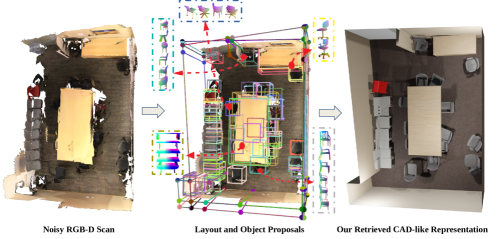
Figure 1: In this paper, we advocate for the use of Monte Carlo Tree Search (MCTS) for 3D scene understanding problems. Given a noisy 3D point cloud recovered from an RGB-D sequence, our approach recovers accurate 3D models and poses for the objects, walls, and floor with minimal training data, even in challenging conditions. We first generate proposals for the layout components and the objects, and rely on Monte Carlo Tree Search (MCTS) adapted to the problem to identify the proposals that best explain the RGB-D sequence. We retrieve correctly the arrangement of chairs on the left-hand side of the scene despite them being close to each other and the thin wall on the top. Our adapted MCTS algorithm has few hyperparameters and can be applied to wide variety of scenes with minimal tuning effort. For visualization purposes only, we texture the objects and the layout using the colors of the 3D points close-by.

1 Introduction

3D scene understanding is a fundamental problem in Computer Vision [41, 53]. In the case of indoor scenes, one usually aims at recognizing the objects and their properties such as their 3D pose and geometry [2, 3, 15], or the room layouts [57, 31, 62, 59, 30, 36, 50, 60, 62, 54, 55], or both [4, 18, 35, 45, 51, 56]. With the development of deep learning approaches, the field has made a remarkable progress. Unfortunately, all recent methods are trained in a supervised way on 3D annotated data. Such a supervised approach has several drawbacks: 3D manual annotations are particularly cumbersome to create and creating realistic virtual 3D scenes also has a high cost [42]. Moreover, supervised methods also tend to generalize poorly to other datasets. Even more importantly, they can only be as good as the training 3D annotations, and mistakes in manual annotations are actually common in existing datasets, as we will show. If one wants to go further and consider more scenes without creating real or synthetic training datasets, it seems important to be able to develop methods that do not rely too much on 3D scenes for training.

Over the history of 3D scene understanding, many non-supervised approaches have already been proposed, including recently to leverage deep learning object detection methods. They typically combine generative models and the optimization of their parameters. Generative methods for 3D scene understanding indeed often involve optimization problems with high complexity, and many optimization tools have thus been investigated, including Markov Random Fields (MRFs) and Conditional Random Fields (CRFs) [22, 52, 32], Markov Chains Monte Carlo (MCMCs) [9, 19, 10, 58], tree search [28], or hill climbing [61, 21]. However, there does not seem to be a clear method of choice: MRFs and CRFs impose strong constraints on the objective function; MCMCs depend on many hyperparameters that are difficult to tune and can result in slow convergence; hill climbing can easily get stuck in a local optimum. The tree search method used by [28] uses a fixed width search tree that can miss good solutions.

In this paper, we advocate for the use of Monte Carlo Tree Search (MCTS) [12, 5], which is a general discrete AI algorithm for learning to play games [46], for optimization in 3D scene understanding problems. We propose to see perception as a (single-player) game, where the goal is to identify the right 3D elements that explain the scene. In such cases where the search problem can be organized into a tree structure which is too large for exhaustive evaluation, MCTS becomes a very attractive option. It also depends on very few easy-to-tune hyperparameters. Moreover, it can be interrupted at any time to return the best solution found so far, which can be useful for robotics applications. A parallel implementation is also possible for high efficiency [8]. In short, MCTS is a powerful optimization algorithm, but to the best of our knowledge, it has never been applied to 3D perception problems.

To apply MCTS to 3D scene understanding, as shown in Fig. Monte Carlo Scene Search for 3D Scene Understanding, we generate proposals for possible objects and layout components using the point cloud generated from the RGB-D sequence, as previous works do from a single RGB-D frame [28, 61]. MCTS can be used to optimize general loss functions, which do not even have to be differentiable. This allows us to rely on a loss function based on an analysis-by-synthesis (or “render-and-compare”) approach to select the proposals that correspond best to the observations. Our loss function compares (non-realistic) renderings of a set of proposals to the input images and can incorporate constraints between the proposals. This turns MCTS into an analysis-by-synthesis method that explores possible sets of proposals for the observations, possibly back-tracking to better solutions when an exploration does not appear promising.

We adapted the original MCTS algorithm to the 3D scene understanding problem to guide it towards the correct solution faster, and call the resulting method “MCSS”, for Monte Carlo Scene Search. First, it is possible to structure the search tree so that it does not contain any impossible solutions, for example, solutions with intersecting proposals. We also enforce the exploration of proposals which are close spatially to proposals in the same path to the root node. Second, we introduce a score based on how the proposal improves the solution locally to increase the efficiency of search.

In practice, we first run MCSS only on the layout proposals to recover the layout. We then run MCSS on the object proposals using the recovered layout. The recovery of the objects thus exploits constraints from the layout, which we found useful as shown in our experiments. In principle, it is possible to run a single MCSS on both the object and layout component proposals, but constraints from the objects did not appear useful to constrain the recovery of the layout for the scenes in ScanNet, which we use to evaluate our approach. We therefore used this two-step approach for simplicity. It is, however, possible that more complex scenes would benefit from a single MCSS running on all the proposals.

Running our method takes a few minutes per scene. This is the same order of magnitude as the time required to acquire an RGB-D sequence covering the scene, but definitively slower than supervised methods. However, our direction could lead to a solution that automatically generates annotations, which could be used to train supervised methods for fast inference. We show in the experiments that our method already retrieves annotations that are sometimes more accurate than existing manual annotations, and that it can be applied to new data without tuning any parameters. Beyond that, MCTS is a very general algorithm, and the approach we propose could be transposed to other perception problems and even lead to an integrated architecture between perception and control, as MCTS has also already been applied to robot motion planning control [25].

2 Related Work

3D scene understanding is an extremely vast topic of the computer vision literature. We focus here on indoor layout and object recovery, as we demonstrate our approach on this specific problem.

2.1 Layout Estimation

The goal of layout estimation is to recover the walls, floor(s), and ceiling(s) of a room or several rooms. This can be very challenging as layout components are often partially or completely occluded by furniture. Hence, many methods resort to some type of prior or supervised learning. The cuboid assumption constraints the room layout to be a box [44, 16, 27]. The Manhattan assumption relaxes somewhat this prior, and enforces the components to be orthogonal or parallel. Many methods working from panoramic images [50, 60, 62] and point clouds [20, 33, 43] rely on such priors. Methods which utilize supervised learning [57, 31, 62, 59, 30, 36, 50, 60, 62, 54, 55] depend on large-scale datasets, the creation of which is a challenge on its own. When performing layout estimation from point clouds as input data [43, 6, 20, 33, 32], one has to deal with incomplete and noisy scans as can be found in the ScanNet dataset [14]. Like previous work [33, 49], we first hypothesize layout component proposals, but relying on MCTS for optimization lets us deal with a large number of proposals and be robust to noise and missing data, without special constraints like the Manhattan assumption.

2.2 3D Object Detection and Model Retrieval

Relevant to our work are techniques to detect objects in the input data and to predict their 3D pose and the 3D model. If 3D data is available, as in our case, this is usually done by first predicting 3D bounding boxes from RGB-D [29, 47, 48] or point cloud data [38, 17, 39, 37, 48] as input. One popular way to retrieve the geometry of objects from indoor point clouds is to predict an embedding and retrieve a CAD model from a database [2, 3, 13, 15, 24].

However, while 3D object category detection and pose estimation from images is difficult due to large variations in appearance, it is also challenging with RGB-D scans due to incomplete depth data. Moreover, in cluttered scenarios, it is still difficult to get all the objects correctly [23]. To be robust, our approach generates many 3D bounding box proposals and multiple possible CAD models for each bounding box. We then rely on MCTS to obtain the optimal combination of CAD models which fits the scene.

2.3 Complete scene reconstruction

Methods for complete scene reconstruction consider both layout and objects. Previous methods fall into two main categories, generative and discriminative methods.

Generative methods often rely on an analysis-by-synthesis approach. A recent example for this is [21] in which the room layout (under cuboid assumption) and alignment of the objects are optimized using a hill-climbing method. Some methods rely on a parse graph as a prior on the underlying structure of the scene [9, 19, 10, 58], and rely on a stochastic Markov Chain Monte Carlo (MCMC) method to find the optimal structure of the parse graph and the component parameters. Such a prior can be very useful to retrieve the correct configuration, unfortunately MCMCs can be difficult to tune so that they work well on all scenes with the same parameters.

Like us, other works deal with an unstructured list of proposals [28, 61], and search for an optimal set which minimizes a fitting cost defined on the RGB-D data. Finding the optimal configuration of components constitutes a subset selection problem. In [61], due to its complexity, it is solved using a greedy hill-climbing search algorithm. In [28], it is solved using beam search on the generated hypothesis tree with a fixed width for efficiency, which can miss good solutions in complex cases. Our approach is similar to [28, 61] as we also first generate proposals and aim at selecting the correct ones, but for the exploration of the search tree, we propose to utilize a variant of Monte Carlo Tree Search, which is known to work well even for very large trees thanks to a guided sampling of the tree.

Discriminative methods can exploit large training datasets to learn to classify scene components from input data such as RGB and RGB-D images [4, 18, 35, 51, 56]. By introducing clever Deep Learning architectures applied to point clouds or voxel-based representations, these methods can achieve very good results. However, supervised methods have practical drawbacks: They are limited by the accuracy of the annotations on which they are trained, and high-quality 3D annotations are difficult to create in practice; generalizing to new data outside the dataset is also challenging. In the experiments, we show that without any manually annotated data, our method can retrieve accurate 3D scene configurations on both ScanNet and our own captures even for cluttered scenes, and with the same hyperparameters.

3 Overview of MCTS

For the sake of completeness, we provide here a brief overview of MCTS. An in-depth survey can be found in [5]. MCTS solves problems of high complexity that can be formalized as tree search by sampling paths throughout the tree and evaluating their scores. Starting from a tree only containing the root node, this tree is gradually expanded in the most promising directions. To identify the most promising solutions (paths from the root node to a leaf node), a score for each created node is evaluated through “simulations” of complete games. A traversal starting from a node can choose to continue with an already visited node with a high score (exploitation) or to try a new node (exploration). MCTS performs a large number of tree traversals, each starting from the root node following four consecutive phases we describe below. The pseudo-code for single-player non-random MCTS, which corresponds to our problem, is given in the supplementary material.

Select. This step selects the next node of the tree to traverse among the children of the current node $\mathcal{N}_{\text{curr}}$. (case 1) If one or several children have not been visited yet, one of them is selected randomly and MCTS moves to the Expand step. (case 2) If all the children have been visited at least once, the next node is selected based on some criterion. The most popular criterion to balance exploitation and exploration is the Upper Confidence Bound (UCB) [1]:

$$\arg\displaystyle\max_{\mathcal{N}\in\mathcal{C}(\mathcal{N}_{\text{curr}})}\lambda_{1}\frac{Q(\mathcal{N})}{n(\mathcal{N})}+\lambda_{2}\cdot\sqrt{\frac{\log n(\mathcal{N}_{curr})}{n(\mathcal{N})}}\>,$$ (1)

where $\mathcal{C}(\mathcal{N}_{\text{curr}})$ is the set of children nodes for the current node, $Q(\mathcal{N})$ is a sum of scores obtained through simulations, and $n(\mathcal{N})$ is the number of times $\mathcal{N}$ is traversed during the search. The selected node is assigned to $\mathcal{N}_{\text{curr}}$, before iterating the Select step. Note that in single-player games, the maximum score is sometimes used in place of the average for the first term, as there is less uncertainty. We tried both options and they perform similarly in our case.

Expand. In case 1, this step expands the tree by adding the randomly selected node to the tree.

Simulate. After the Expand step, many “simulations” of the game are run to assign the new node $\mathcal{N}$ a score, stored in $Q(\mathcal{N})$. Each simulation follows a randomly-chosen path from the new node until the end of the game. The score can be for example the highest score obtained by a simulation at the end of the game.

Update. After the Simulate step, the score is also added to the $Q$ values of the ancestors of $\mathcal{N}$. The next MCTS iteration will then traverse the tree from the root node using the updated scores.

After a chosen number of iterations, in the case of non-random single-player games, the solution returned by the algorithm is the simulation that obtained the best score for the game.

4 Approach

In this section, we first derive our objective and then explain how we adapt MCTS to solve it efficiently.

4.1 Formalization

Given a set $\mathcal{I}=\{(I_{i},D_{i})\}_{i=1}^{N_{V}}$ of $N_{V}$ registered RGB images and depth maps of a 3D scene, we want to find 3D models and their poses for the objects and walls that constitute the 3D scene. This can be done by looking for a set of objects and layout elements from a pool of proposals, $\hat{\mathcal{O}}$ that maximizes the posterior given the observations in $\mathcal{I}$:

$$\hat{\mathcal{O}}=\arg\max_{\mathcal{O}}P(\mathcal{O}\;\lvert\;\mathcal{I})=\arg\max_{\mathcal{O}}\log P(\mathcal{O}\;\lvert\;\mathcal{I})\>.$$ (2)

The set of object proposals contains potential 3D model candidates for each object in the scene, along with its corresponding pose. The same 3D model for an object but under two different poses constitutes two proposals. The set of layout proposals models potential layout candidates as planar 3D polygons. More details about the proposal generation is provided later in Section 4.3.

Using the images rather than only the point cloud is important, as shown in [37] for example, as many parts of a scanned scene can be missing from the point cloud, when the RGB-D camera did not return depth values for them (this happens for dark and reflective materials, for example). Assuming the $I_{i}$ and $D_{i}$ are independent, $\log P(\mathcal{O}\;\lvert\;\mathcal{I})$ is proportional to:

$$\sum_{i}\big{(}\log P(I_{i}\;\lvert\;\mathcal{O})+\log P(D_{i}\;\lvert\;\mathcal{O})\big{)}+\log P(\mathcal{O})\>.$$ (3)

$P(I_{i}\;\lvert\;\mathcal{O})$ and $P(D_{i}\;\lvert\;\mathcal{O})$ are the likelihoods of our observations. To evaluate them, we compare $I_{i}$ and $D_{i}$ with (non-realistic) renderings of the objects and layout elements in $\mathcal{O}$ from the same camera poses as the $I_{i}$ and $D_{i}$. For $P(I_{i}\;\lvert\;\mathcal{O})$, we render the objects and layout elements in $\mathcal{O}$ using their class indices in place of colors and compare the result with a semantic segmentation of image $I_{i}$. To evaluate $P(D_{i}\;\lvert\;\mathcal{O})$, we render a depth map for the objects and layout elements in $\mathcal{O}$ and compare it with $D_{i}$. More formally, we model $\log P(I_{i}\;\lvert\;\mathcal{O})+\log P(D_{i}\;\lvert\;\mathcal{O})$ by:

$$s_{i}(\mathcal{O})=\lambda_{I}\sum_{c}S_{i}(c)\cdot S_{i}^{R}(c)-\lambda_{D}|D_{i}-D_{i}^{R}|\>,$$ (4)

up to some additive constant that does not change the optimization problem in Eq. (2). The $S_{i}(c)$ are segmentation confidence maps for classes $c\in\{\text{wall},\text{floor},\text{chair},\text{table},\text{sofa},\text{bed}\}$ obtained by semantic segmentation of $I_{i}$ (we use MSEG [26] for this); the $S_{i}^{R}(c)$ are rendered segmentation maps (a pixel in $S_{i}^{R}(c)$ has value 1 if lying on an object or layout element of class $c$, 0 otherwise). $D_{i}^{R}$ is the rendered depth map of the objects and layout elements in $\mathcal{O}$.

Given a set $\mathcal{O}$, $s_{i}(\mathcal{O})$ can be computed efficiently by pre-rendering a segmentation map and a depth map for each proposal independently: $D_{i}^{R}$ can be constructed by taking for each pixel the minimal depth over the pre-rendered depth maps for the proposals in $\mathcal{O}$. $S_{i}^{R}(c)$ can be constructed similarly using both the pre-rendered segmentation and depth maps.

Fig. 2 shows an example of $S_{i}$, $S_{i}^{R}$, $D_{i}$, and $D_{i}^{R}$. Note that our approach considers all the objects together and takes naturally into account the occlusions that may occur between them, which is one of the advantages of analysis-by-synthesis approaches. More sophisticated ways to evaluate the observations likelihoods could be used, but this simple method already yields very good results.

(a)		(b)
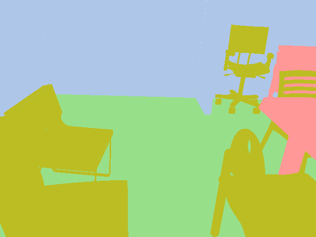
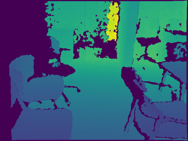
(c)		(d)

Figure 2: Examples for (a) $S_{i}$, (b) $S_{i}^{R}$, (c) $D_{i}$, (d) $D_{i}^{R}$.

$P(\mathcal{O})$ in Eq. (3) is a prior term on the set $\mathcal{O}$. We currently use it to prevent physically impossible solutions only. In practice, the proposals are not perfectly localised and we tolerate some intersections. When the Intersection-Over-Union between two objects is smaller than a threshold, we tolerate the intersection but still penalize it. More formally, in this case, we model $\log P(\mathcal{O})$ by

$$s^{p}(\mathcal{O})=-\lambda_{P}\sum_{O,O^{\prime}\in\mathcal{O},O\neq O^{\prime}}\text{IoU}(O,O^{\prime})\>$$ (5)

up to some additive constant. IoU is the intersection-over-Union between the 3D models for objects $O_{j}$ and $O_{k}$. In practice, we compute it using a voxel representation of the 3D models. When the Intersection-over-Union between two object proposals is above a threshold, we take $P(\mathcal{O})=0$, the two proposals are incompatible. In practice, we use a threshold of 0.3. We consider two special cases where this is not true: chair-table and sofa-table intersections. In these cases, we first identify the horizontal surface on which the intersection occurs (surface of the table, seat of the sofa) and determine the amount of intersection by calculating the distance of the intersecting point to nearest edge of the horizontal surface. The amount of intersection is normalized by the dimension of the horizontal surface and a ratio more than 0.3 is considered incompatible.

Similarly, when two layout proposals intersect or when a layout proposal and an object proposal intersect, we take also $P(\mathcal{O})=0$. In contrast to object proposals where small intersections are still tolerated, we do not tolerate any intersections for the layout proposals as their locations tend to be predicted more accurately.

As discussed in the introduction, to find a set $\hat{\mathcal{O}}$ that maximizes Eq. (2), we build a pool $\mathcal{O}_{\text{pool}}$ of proposals, and select $\hat{\mathcal{O}}$ as the subset of $\mathcal{O}_{\text{pool}}$ that maximizes the global score $S(\mathcal{O})=\sum_{i}s_{i}(\mathcal{O})+s^{P}(\mathcal{O})$. We empirically set $\lambda_{I}=\lambda_{D}$ = 1 and $\lambda_{P}=2.5$ in our experiments to balance the three terms in Eq. (3).

4.2 Monte Carlo Scene Search

We now explain how we adapted MCTS to perform an efficient optimization of the problem in Eq. (3). We call this variant “Monte Carlo Scene Search” (MCSS).

4.2.1 Tree Structure

In the case of standard MCTS, the search tree follows directly from the rules of the game. We define the search tree explored by MCSS to adapt to the scene understanding problem and to allow for an efficient exploration as follows.

Proposal fitness. Each proposal $\mathcal{P}$ is assigned a fitness value obtained by evaluating $s_{i}$ in Eq. (4) only over the pixel locations where the proposal reprojects. Note that this fitness is associated with a proposal and not a node. This fitness will guide both the definition and the exploration of the search tree during the simulations.

Except for the root node, a node $\mathcal{N}$ in the scene tree is associated with a proposal $\mathcal{P}(\mathcal{N})$ from the pool $\mathcal{O}_{\text{pool}}$. Each path from the root node to a leaf node thus corresponds to a set of proposals $\mathcal{O}$ that is a potential solution to Eq. (2). We define the tree so that no path can correspond to an impossible solution to set $\mathcal{O}$ with $P(\mathcal{O})=0$. This simplifies the search space to the set of possible solutions only. We also found that considering first proposals that are close spatially to proposals in a current path significantly speeds up the search, and we also organize the tree by spatial neighbourhood. The child nodes of the root node are made of a node containing the proposal $O$ with the highest fitness among all proposals, and a node for each proposal that is incompatible with $O$. The child nodes of every other node $\mathcal{N}$ contain the closest proposal $O$ to the proposal in $\mathcal{N}$, and the proposals $O^{\prime}$ incompatible with $O$, under the constraint that $O$ and proposals $O^{\prime}$ are compatible with all the proposals in $\mathcal{N}$ and its ancestors.

Two layout proposals are considered incompatible if they intersect and are not spatial neighbours. They are spatial neighbors if they share an edge and are not on the same 3D plane. Therefore, if $\mathcal{P}(\mathcal{N})$ is a layout proposal, the children nodes are always layout components that are connected by an edge to $\mathcal{P}(\mathcal{N})$. By doing so, we enforce that each path in the tree enforces structured layouts, the layout components are connected. Note that this strategy will miss disconnected layout structures such as pillars in the middle of a room but works well on ScanNet.

In the case of objects, the spatial distance between two object proposals is computed by taking the Euclidean distance between the centers of the 3D bounding boxes. The incompatibility between two object proposals is determined as explained in Section 4.1. Since all the object proposals in the children of a node may be all incorrect, we add a special node that does not contain a proposal to avoid having to select an incorrect proposal. The children nodes of the special node are based on the proximity to its parent node excluding the proposals in its sibling nodes.

As mentioned in the introduction, we first run MCSS on the layout component proposals only to select the correct layout components first. Then, we run MCSS on the object proposals, with the selected layout components in $\mathcal{O}$. The selection of the object proposals therefore benefits from the recovered layout.

4.2.2 Local node scores

Usually with MCTS, $Q$ in the UCB criterion given in Eq. (1) and stored in each node is taken as the sum of the game final scores obtained after visiting the node. We noticed during our experiments that exploration is more efficient if $Q$ focuses more on views where the proposal in the node is visible. Thus, in MCSS, after a simulation returns $\mathcal{O}$, the score $s$ is added to $Q$ of a node containing a proposal $O$. $s$ is a local score calculated as follows to focus on $O$:

$$s=\frac{1}{\sum_{i}w_{i}(O)}\sum_{i}w_{i}(O)s_{i}(\mathcal{O})+\lambda_{p}s^{P}(O,\mathcal{O})\>,$$ (6)

where $w_{i}(O)=1$ if $O$ is visible in view $i$ and 0 otherwise, and

$$s^{p}(O,\mathcal{O})=-\sum_{O^{\prime}\in\mathcal{O},O\neq O^{\prime}}\text{IoU}(O,O^{\prime})\>.$$ (7)

4.2.3 Running simulations

While running the simulations, instead of randomly picking the nodes, we use a “roulette wheel selection” based on their proposals: the probability for picking a node is directly proportional to the fitness of the proposal it contains.

4.2.4 MCSS output

Besides the tree definition and the local score given in Eq. (6) used in the Select criterion, MCSS runs as MCTS to return the best set $\mathcal{O}$ of proposals found by the simulations according to the final score $S(\mathcal{O})=\sum_{i}s_{i}(\mathcal{O})+s^{P}(\mathcal{O})$. In practice, we perform 20,000 iterations of MCSS.

4.3 Generating Proposals

We resort here on off-the-shelf techniques. For the object proposals, we first create a set of synthetic point clouds using ShapeNet [7] CAD models and the ScanNet dataset [14] (we provide more details in the suppl. mat.). We train VoteNet [38] on this dataset to generate 3D bounding boxes with their predicted classes. Note that we do not need VoteNet to work very well as we will prune the false positives anyway, which makes the approach generalizable. Using simple heuristics, we create additional 3D bounding boxes by splitting and merging the detections from VoteNet, which we found useful to deal with cluttered scenes. We also train MinkowskiNet [11] on the same synthetic dataset which we use to remove the points inside the bounding boxes that do not belong to the Votenet predicted class. We then trained a network based on PointNet++ [40] on the same synthetic data to predict an embedding for a CAD model from ShapeNet [7] and a 6D pose+scale from samplings of the remaining points. Different samplings result in slightly different embeddings and we generate a proposal with each of the corresponding CAD models. We refine the pose and scale estimates by performing a small grid search around the predicted values using the Chamfer distance between the CAD model and the point cloud.

For the layout component proposals, we use the semantic segmentation by MinkowskiNet to extract the 3D points on the layout from the point cloud and rely on a simple RANSAC procedure to fit 3D planes. Like previous works [33, 34, 61, 49], we compute the intersections between these planes to obtain 3D polygons, which we use as layout proposals. We also include the planes of the point cloud’s 3D bounding box faces to handle incomplete scans: for example, long corridors are never scanned completely in ScanNet.

5 Evaluation

We present here the evaluation of our method. We also provide an ablation study to show the importance of our modifications to MCTS and of the use of the retrieved layouts when retrieving the objects.

Fig. 4 shows the output of our method on a custom scan, and more qualitative results are provided in the suppl. mat.

(a)

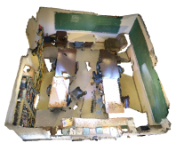
(b)

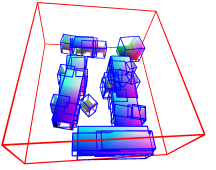
(c)

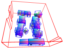
(d)

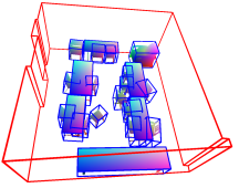
Figure 3: (a) An RGB-D scan from the ScanNet dataset [14]. (b) Output of the VoteNet-based baseline method for the objects, together with the layout annotations from [4]. Many objects retrieved by the baseline method are incorrect; the layout annotations lack some details. (c) Objects and layout prediction by our MCSS method. Our predicted layout has much more details than the manual annotations. (d) Objects annotations from [2] together with our manual layout annotations. The supp. mat. provides more visualizations.

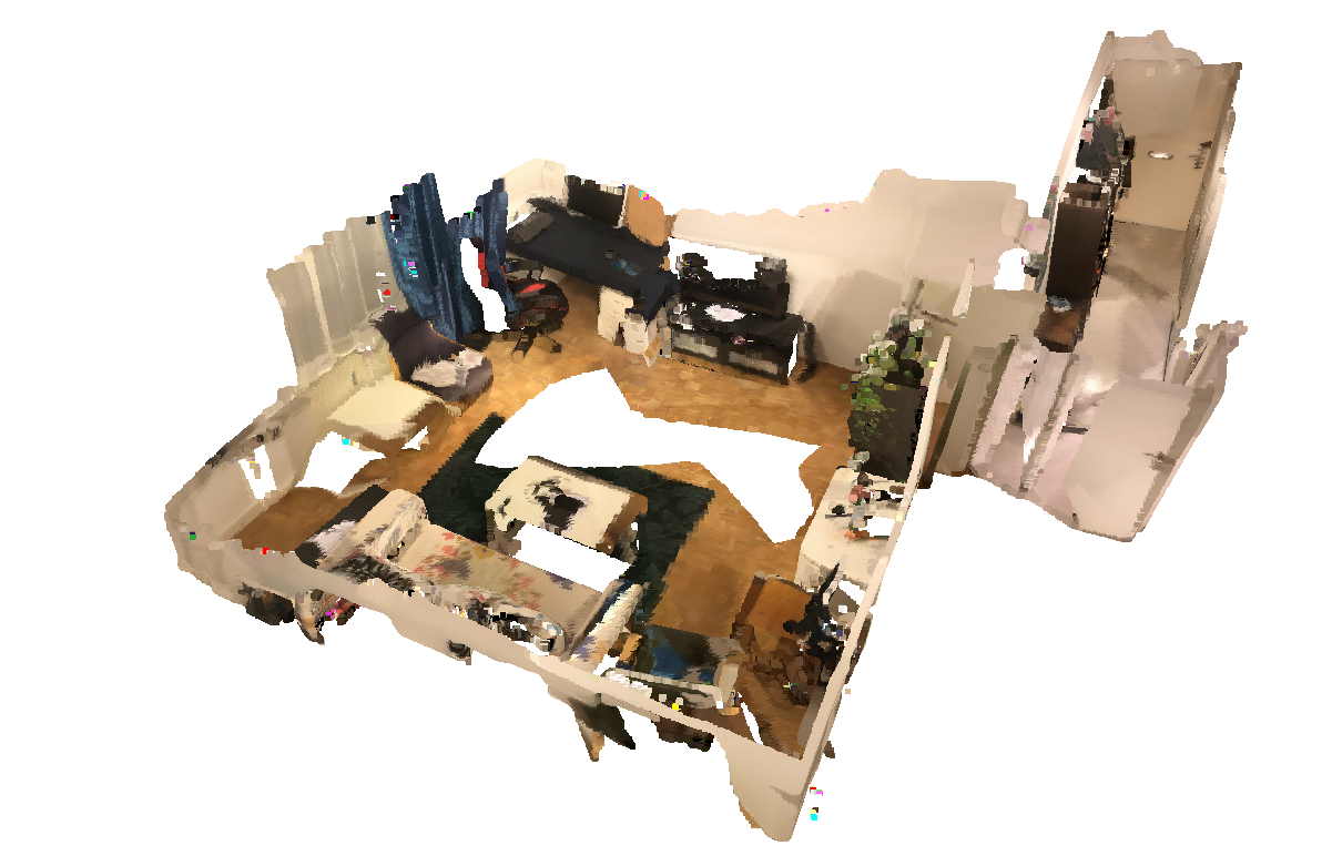
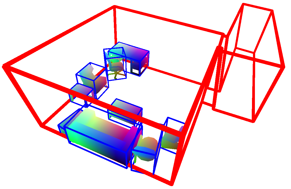
(a)	(b)

Figure 4: Generalization to other datasets. (a) We captured an RGB-D scan of an apartment with a hallway and a living space, and many furniture. (b) Objects and layout found by our MCSS method. More results are provided in the suppl. mat.

5.1 Layouts

We first evaluate the ability of MCSS to recover general layouts on validation scenes from the SceneCAD dataset [2] that provides layout annotations for noisy RGBD scans from the ScanNet dataset [14]. MCSS outperforms the SceneCAD method by a quite substantial margin on the corner recall metric, with 84.8% compared to 71%. However, as shown in Fig. 3(b), the SceneCAD annotations lack details, which hurts the performance of our method on other metrics as it recovers details not in the manual annotations.

Hence, we relabelled the same set of scenes from the SceneCAD dataset with more details. As proposed in the SceneCAD paper, a predicted corner is considered to be matching to the ground truth corner if it is within $40cm$ radius. We further adjust this criterion: if multiple predicted corners are within this radius, a single corner that is closest to the ground truth is taken and a predicted corner can be assigned to only one ground truth corner. We also compute the polygons’ Intersection-Over-Union (IOU) metric from [49] after projecting the retrieved polygons to their ground truth polygons. Table 1 compares the layouts retrieved by our approach to the SceneCAD annotations. These annotations obtain very high corner precision, as most of the annotated corners are indeed correct, but low corners recall and polygon IOU because of the missing details. By contrast, our method recovers most corners which results in high recall without generating wrong ones, as is visible from the high precision. Our approach does well to recover general room structure as shown by the polygon IOU value. We show in Fig. 3, 4 and suppl. mat. that our method successfully recovers a variety of layout configurations. Most errors come from the fact that components might be completely invisible in the scene in all of the views as our proposal generation is not intended for this special case.

	All Scenes			Non-Cuboid Scenes
	Prec	Rec	IOU	Prec	Rec	IOU
SceneCAD GT	91.2	80.4	75.0	90.8	73.3	66.1
MCSS (Ours)	85.5	86.1	75.8	83.5	80.4	70.4

Table 1: Comparison between manual SceneCAD layout annotations and layouts retrieved by our method, on our more detailed layout annotations.

5.2 Objects

We evaluate our method on the subset of scenes from both the test set and validation set of Scan2CAD [2]. We consider 95 scenes in the test set and 126 unique scenes in the validation which contains at least one object from the chair, sofa, table, bed categories. A complete list of the scenes used in our evaluations is provided in the suppl. mat.

We first consider a baseline which uses Votenet [38] for object detection and retrieves a CAD model and its pose for each 3D bounding box using the same network used for our proposals. The performance of this baseline will show the impact of not using multiple proposals for both object detection and model retrieval.

We use the accuracy metric defined in [2] for evaluations on the test set and compare with three methods ( Scan2CAD [2], E2E [3], and SceneCAD [4]) in Table 3. While our method is trained only on simple synthetic data, it still outperforms Scan2CAD and E2E on the chair and sofa categories. The loower performance on the table category is due to inconsistent manual annotations: Instance level annotation of a group of tables from an incomplete point cloud is challenging and this results in inconsistent grouping of tables as shown in Fig. 5. Although we achieve plausible solutions in these scenarios, it is difficult to obtain similar instance-level detection as the manual annotations. Moreover, SceneCAD learns to exploit object-object and object-layout support relationships, which significantly improves the performance. Our approach does not exploit such constraints yet, but they could be integrated in the objective function’s prior term in future work for benefits.

Table 4 compares the Chamfer distance between the objects we retrieve and the manually annotated point cloud of the object on the validation set of ScanNet. This metric captures the accuracy of the retrieved CAD models. The models we retrieve for chair and sofa are very similar to the models chosen for the manual annotations as the Chamfer distances have the same order of magnitude.

Table 2 reports the precision and recall for the oriented 3D bounding boxes for the pool of object proposals, for the set of proposals selected by MCSS, and for the baseline. MCSS improves the precision and recall from the baseline in all 4 object categories. The recall remains similar while the precision improves significantly. This proves that our method efficiently rejects all incorrect proposals. Our qualitative results in Fig. 3 and 5 show the efficacy of MCSS in rejecting many incorrect proposals compared to the baseline method while also retaining the correct CAD models that are similar to ground truth. We even retrieve objects missing from the annotations.

	IOU Th.	Chair		Sofa		Table		Bed
		Prec	Rec	Prec	Rec	Prec	Rec	Prec	Rec
All proposals	0.50	0.06	0.92	0.05	0.93	0.05	0.68	0.16	0.93
	0.75	0.04	0.59	0.04	0.56	0.03	0.46	0.08	0.48
Baseline	0.50	0.70	0.85	0.77	0.80	0.66	0.56	0.74	0.74
	0.75	0.19	0.29	0.31	0.39	0.24	0.30	0.30	0.41
MCSS (Ours)	0.50	0.75	0.87	0.79	0.93	0.65	0.59	0.86	0.86
	0.75	0.27	0.32	0.42	0.42	0.34	0.30	0.41	0.44

Table 2: Evaluation of object model retrieval and alignment with bounding box IOU thresholds 0.5 and 0.75. The recall for our method is similar to the recall with all proposals while precision is better than the baseline method. Our method efficiently rejects all the incorrect proposals.

Method	Obj-Obj Support	Chair	Sofa	Table
Baseline	No	42.02	27.70	18.52
Scan2CAD [2]	No	44.26	30.66	30.11
E2E [3]	No	73.04	76.92	48.15
SceneCAD [4]	Yes	81.26	82.86	45.60
MCSS (Ours)	No	74.32	78.70	24.28

Table 3: Comparison of object alignment on the Scan2CAD benchmark. The metrics for bed alone are not provided by the benchmark and hence not shown. SceneCAD uses inter-object support relations to improve their results from E2E. We do not have access to these relationships and hence mostly compare with E2E and Scan2CAD. The lower accuracy for table seems to be due to the dataset bias discussed in Fig. 5.

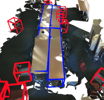
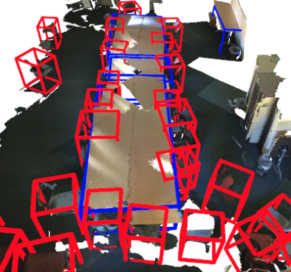
(a) Manual Annotations	(b) MCSS (ours)

Figure 5: Manual annotation of incomplete point clouds is difficult and groups of tables are often annotated incorrectly in the Scan2CAD dataset, creating a dataset bias. For example, in (a), there should be 8 tables instead of 4 in the annotations. This hurts our performance for the table category, though we achieve plausible solutions (b). Note that we also often retrieve more objects than in the annotations.

Method	Chair	Sofa	Table	Bed
Baseline	2.6	11.0	14.2	26.3
MCSS (Ours)	1.8	7.4	12.8	16.2
Manual annotations [2]	2.0	5.2	5.5	9.4

Table 4: Comparison of one-way Chamfer distance (in mm) between scan points and retrieved models on the validation set of Scan2CAD. Our retrieved models are close to manual annotations for chair and sofa even though we use only synthetic point clouds for model retrieval.

5.3 Ablation Study

Importance of local score (Eq. 6).

In Fig. 6, we plot the best score $S(\mathcal{O})$ found so far with respect to the MCTS iteration, in the case of a complex scene for layout recovery and object recovery, when using the simulation score $S(\mathcal{O})$ or the local score $s$ given in Eq. (6) to update the $Q$ of the nodes. We use the selection strategy of Eq. (1) in both of these scenarios. We also plot the best score for a random tree search. Using the local score speeds up the convergence to a better solution, achieving on an average 9% and 15% higher global scores for layouts and objects, respectively. Compared to random tree search, our method achieves 15% and 42% higher scores for layout and objects, respectively. We consider 12 challenging scenes for this experiment.

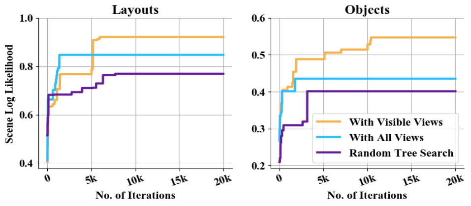
	Search Method Node Score Simulation With Visible Views Eq. (6) Roulette Wheel With All Views $\sum_{i}s_{i}(\mathcal{O})+s^{P}(\mathcal{O})$ Roulette Wheel Random Search 0 Uniform Probability

Figure 6: Best score $S(O)=\big{(}\sum_{i}s_{i}(\mathcal{O})+s^{P}(\mathcal{O})\big{)}$ found so far for layout and objects over MCSS iterations. Using the local score given in Eq. (6) results in much faster and better convergence.

Importance of layout for retrieving objects.

Table 5 shows the effect of using the estimated layout in the terms of Eq. (4) while running MCSS on objects. We considered 12 challenging scenes mainly containing chairs and tables for this experiment and use the same precision and recall metrics as in Table 2. Using the layout clearly helps by providing a better evaluation of image and depth likelihoods.

	Chair		Table
	Prec	Rec	Prec	Rec
Without layout	0.58	0.61	0.48	0.34
With layout	0.65	0.84	0.66	0.58

Table 5: Impact of using the estimated layout when running MCSS for object retrieval.

Acknowledgments. This work was supported by the Christian Doppler Laboratory for Semantic 3D Computer Vision, funded in part by Qualcomm Inc.

References

- [1] Peter Auer, Nicolo Cesa-Bianchi, and Paul Fischer. Finite-time Analysis of the Multiarmed Bandit Problem. Machine Learning, 47(2):235–256, 2002.
- [2] Armen Avetisyan, Manuel Dahnert, Angela Dai, Manolis Savva, Angel X. Chang, and Matthias Nießner. Scan2CAD: Learning CAD Model Alignment in RGB-D Scans. In CVPR, June 2019.
- [3] Armen Avetisyan, Angela Dai, and Matthias Nießner. End-to-End CAD Model Retrieval and 9DoF Alignment in 3D Scans. In ICCV, 2019.
- [4] Armen Avetisyan, Tatiana Khanova, Christopher Choy, Denver Dash, Angela Dai, and Matthias Nießner. SceneCAD: Predicting Object Alignments and Layouts in RGB-D Scans. In ECCV, Aug. 2020.
- [5] Cameron Browne, Edward Powley, Daniel Whitehouse, Simon Lucas, Peter Cowling, Philipp Rohlfshagen, Stephen Tavener, Diego Perez liebana, Spyridon Samothrakis, and Simon Colton. A Survey of Monte Carlo Tree Search Methods. IEEE Transactions on Computational Intelligence and AI in Games, 4:1:1–43, 2012.
- [6] Ricardo Cabral and Yasutaka Furukawa. Piecewise Planar and Compact Floorplan Reconstruction from Images. In CVPR, 2014.
- [7] Angel X. Chang, Thomas A. Funkhouser, Leonidas J. Guibas, Pat Hanrahan, Qi-Xing Huang, Zimo Li, Silvio Savarese, Manolis Savva, Shuran Song, Hao Su, Jianxiong Xiao, Li Yi, and Fisher Yu. ShapeNet: An Information-Rich 3D Model Repository. CoRR, abs/1512.03012, 2015.
- [8] Guillaume M. J-B Chaslot, Mark H. M. Winands, and Jaap Van den herik. Parallel Monte-Carlo Tree Search. In International Conference on Computers and Games, 2008.
- [9] Yixin Chen, Siyuan Huang, Tao Yuan, Siyuan Qi, Yixin Zhu, and Song-Chun Zhu. Holistic++ Scene Understanding: Single-View 3D Holistic Scene Parsing and Human Pose Estimation with Human-Object Interaction and Physical Commonsense. In ICCV, 2019.
- [10] Wongun Choi, Yu-Wei Chao, Caroline Pantofaru, and Silvio Savarese. Understanding indoor scenes using 3d geometric phrases. In CVPR, 2013.
- [11] Christopher Choy, JunYoung Gwak, and Silvio Savarese. 4D Spatio-Temporal ConvNets: Minkowski Convolutional Neural Networks. In CVPR, 2019.
- [12] Rémi Coulom. Efficient Selectivity and Backup Operators in Monte-Carlo Tree Search. In International Conference on Computers and Games, 2006.
- [13] Manuel Dahnert, Angela Dai, Leonidas Guibas, and Matthias Nießner. Joint Embedding of 3D Scan and CAD Objects. In ICCV, 2019.
- [14] Angela Dai, Angel X. Chang, Manolis Savva, Maciej Halber, Thomas Funkhouser, and Matthias Nießner. ScanNet: Richly-Annotated 3D Reconstructions of Indoor Scenes. In CVPR, 2017.
- [15] Alexander Grabner, Peter M. Roth, and Vincent Lepetit. 3D Pose Estimation and 3D Model Retrieval for Objects in the Wild. In CVPR, 2018.
- [16] Varsha Hedau, Derek Hoiem, and David Forsyth. Recovering the Spatial Layout of Cluttered Rooms. In ICCV, 2009.
- [17] Ji Hou, Angela Dai, and Matthias Nießner. 3D-SIS: 3D Semantic Instance Segmentation of RGB-D Scans. In CVPR, 2019.
- [18] Siyuan Huang, Siyuan Qi, Yinxue Xiao, Yixin Zhu, Ying Nian Wu, and Song-Chun Zhu. Cooperative Holistic Scene Understanding: Unifying 3D Object, Layout, and Camera Pose Estimation. In NeurIPS, 2018.
- [19] Siyuan Huang, Siyuan Qi, Yixin Zhu, Yinxue Xiao, Yuanlu Xu, and Song-Chun Zhu. Holistic 3D Scene Parsing and Reconstruction from a Single RGB Image. In ECCV, 2018.
- [20] Satoshi Ikehata, Hang Yang, and Yasutaka Furukawa. Structured Indoor Modeling. In ICCV, 2015.
- [21] Hamid Izadinia, Qi Shan, and Steven M. Seitz. Im2CAD. In CVPR, 2017.
- [22] Hema Swetha Koppula, Abhishek Anand, Thorsten Joachims, and Ashutosh Saxena. Semantic Labeling of 3D Point Clouds for Indoor Scenes. In NIPS, 2011.
- [23] Nilesh Kulkarni, Ishan Misra, Shubham Tulsiani, and Abhinav Gupta. 3D-RelNet: Joint Object and Relational Network for 3D Prediction. In ICCV, 2019.
- [24] Wei-Cheng Kuo, A. Angelova, Tsung-Yi Lin, and Angela Dai. Mask2CAD: 3D Shape Prediction by Learning to Segment and Retrieve. In arXiv, 2020.
- [25] Yann Labbé, Sergey Zagoruyko, Igor Kalevatykh, Ivan Laptev, Justin Carpentier, Mathieu Aubry, and Josef Sivic. Monte-Carlo Tree Search for Efficient Visually Guided Rearrangement Planning. IEEE Robotics and Automation Letters, 2020.
- [26] John Lambert, Zhuang Liu, Ozan Sener, James Hays, and Vladlen Koltun. MSeg: A Composite Dataset for Multi-Domain Semantic Segmentation. In CVPR, 2020.
- [27] Chen-Yu Lee, Vijay Badrinarayanan, Tomasz Malisiewicz, and Andrew Rabinovich. RoomNet: End-To-End Room Layout Estimation. In ICCV, 2017.
- [28] David C. Lee, Abhinav Gupta, Martial Hebert, and Takeo Kanade. Estimating Spatial Layout of Rooms Using Volumetric Reasoning About Objects and Surfaces. In NeurIPS, 2010.
- [29] Dahua Lin, Sanja Fidler, and Raquel Urtasun. Holistic Scene Understanding for 3D Object Detection with RGBD Cameras. In ICCV, 2013.
- [30] Chen Liu, Jiaye Wu, and Yasutaka Furukawa. FloorNet: A Unified Framework for Floorplan Reconstruction from 3D Scans. In ECCV, 2018.
- [31] Chen Liu, Jiajun Wu, Pushmeet Kohli, and Yasutaka Furukawa. Raster-To-Vector: Revisiting Floorplan Transformation. In ICCV, 2017.
- [32] Claudio Mura, Oliver Mattausch, and Renato Pajarola. Piecewise-planar Reconstruction of Multi-room Interiors with Arbitrary Wall Arrangements. Computer Graphics Forum, 2016.
- [33] Srivathsan Murali, Pablo Speciale, Martin R. Oswald, and Marc Pollefeys. Indoor Scan2BIM: Building Information Models of House Interiors. In IROS, 2017.
- [34] Liangliang Nan and Peter Wonka. PolyFit: Polygonal Surface Reconstruction from Point Clouds. In ICCV, 2017.
- [35] Yinyu Nie, Xiaoguang Han, Shihui Guo, Yujian Zheng, Jian Chang, and Jian Jun Zhang. Total3DUnderstanding: Joint Layout, Object Pose and Mesh Reconstruction for Indoor Scenes from a Single Image. In CVPR, June 2020.
- [36] G. Pintore and M. Agus. AtlantaNet: Inferring the 3D Indoor Layout from a Single 360 Image Beyond the Manhattan World Assumption. In ECCV, 2020.
- [37] Charles R. Qi, Xinlei Chen, Or Litany, and Leonidas J. Guibas. ImVoteNet: Boosting 3D Object Detection in Point Clouds with Image Votes. In CVPR, 2020.
- [38] Charles R. Qi, Or Litany, Kaiming He, and Leonidas J. Guibas. Deep Hough Voting for 3D Object Detection in Point Clouds. In ICCV, 2019.
- [39] Charles R. Qi, Wei Liu, Chenxia Wu, Hao Su, and Leonidas J. Guibas. Frustum PointNets for 3D Object Detection from RGB-D Data. In CVPR, 2018.
- [40] Charles R. Qi, Li Yi, Hao Su, and Leonidas J. Guibas. PointNet++: Deep Hierarchical Feature Learning on Point Sets in a Metric Space. In arXiv, 2017.
- [41] Lawrence Roberts. Machine Perception of Three-Dimensional Solids. PhD thesis, MIT, 1965.
- [42] Mike Roberts and Nathan Paczan. Hypersim: A Photorealistic Synthetic Dataset for Holistic Indoor Scene Understanding. In arXiv, 2020.
- [43] Victor Sanchez and Avideh Zakhor. Planar 3D Modeling of Building Interiors from Point Cloud Data. In ICIP, 2012.
- [44] Alexander G. Schwing, Tamir Hazan, Marc Pollefeys, and Raquel Urtasun. Efficient Structured Prediction for 3D Indoor Scene Understanding. In CVPR, 2012.
- [45] Tianjia Shao, Aron Monszpart, Youyi Zheng, Bongjin Koo, Weiwei Xu, Kun Zhou, and Niloy J Mitra. Imagining the Unseen: Stability-based Cuboid Arrangements for Scene Understanding. ACM Transactions on Graphics, 2014.
- [46] David Silver, Thomas Hubert, Julian Schrittwieser, Ioannis Antonoglou, Matthew Lai, Arthur Guez, Marc Lanctot, Laurent Sifre, Dharshan Kumaran, Thore Graepel, Timothy Lillicrap, Karen Simonyan, and Demis Hassabis. A General Reinforcement Learning Algorithm That Masters Chess, Shogi, and Go through Self-Play. Science, 362(6419):1140–1144, 2018.
- [47] Shuran Song and Jianxiong Xiao. Sliding Shapes for 3D Object Detection in Depth Images. In ECCV, 2014.
- [48] Shuran Song and Jianxiong Xiao. Deep Sliding Shapes for Amodal 3D Object Detection in RGB-D Images. In CVPR, 2016.
- [49] Sinisa Stekovic, Shreyas Hampali, Mahdi Rad, Sayan Deb Sarkar, Friedrich Fraundorfer, and Vincent Lepetit. General 3D Room Layout from a Single View by Render-and-Compare. In ECCV, 2020.
- [50] Cheng Sun, Chi-Wei Hsiao, Min Sun, and Hwann-Tzong Chen. HorizonNet: Learning Room Layout with 1D Representation and Pano Stretch Data Augmentation. In CVPR, 2019.
- [51] Shubham Tulsiani, Saurabh Gupta, David Fouhey, Alexei A. Efros, and Jitendra Malik. Factoring Shape, Pose, and Layout from the 2D Image of a 3D Scene. In CVPR, 2018.
- [52] Shenlong Wang, Sanja Fidler, and Raquel Urtasun. Holistic 3D Scene Understanding from a Single Geo-tagged Image. In CVPR, 2015.
- [53] Yoram Yakimovsky and Jerome A. Feldman. A Semantics-Based Decision Theory Region Analyzer. IJCAI, 1973.
- [54] Wei Zeng, Sezer Karaoglu, and Theo Gevers. Joint 3D Layout and Depth Prediction from a Single Indoor Panorama Image. In ECCV, 2020.
- [55] Weidong Zhang, Wei Zhang, and Yinda Zhang. GeoLayout: Geometry Driven Room Layout Estimation Based on Depth Maps of Planes. In ECCV, 2020.
- [56] Yinda Zhang, Shuran Song, Ping Tan, and Jianxiong Xiao. PanoContext: A Whole-Room 3D Context Model for Panoramic Scene Understanding. In ECCV, 2014.
- [57] Yinda Zhang, Fisher Yu, Shuran Song, Pingmei Xu, Ari Seff, and Jianxiong Xiao. Large-Scale Scene Understanding Challenge: Room Layout Estimation. In CVPR, 2015.
- [58] Yibiao Zhao and Song-Chun Zhu. Scene Parsing by Integrating Function, Geometry and Appearance Models. In CVPR, 2013.
- [59] Jia Zheng, Junfei Zhang, Jing Li, Rui Tang, Shenghua Gao, and Zihan Zhou. Structured3D: A Large Photo-Realistic Dataset for Structured 3D Modeling. In ECCV, 2020.
- [60] Chuhang Zou, Alex Colburn, Qi Shan, and Derek Hoiem. LayoutNet: Reconstructing the 3D Room Layout from a Single RGB Image. In CVPR, 2018.
- [61] Chuhang Zou, Ruiqi Guo, Zhizhong Li, and Derek Hoiem. Complete 3D Scene Parsing from an RGBD Image. IJCV, 2019.
- [62] Chuhang Zou, Jheng-Wei Su, Chi-Han Peng, Alex Colburn, Qi Shan, Peter Wonka, Hung-Kuo Chu, and Derek Hoiem. 3D Manhattan Room Layout Reconstruction from a Single 360 Image. In arXiv, 2019.