Contents, Contexts, and Basics of Contextuality

Abstract

This is a non-technical introduction into theory of contextuality. More precisely, it presents the basics of a theory of contextuality called Contextuality-by-Default (CbD). One of the main tenets of CbD is that the identity of a random variable is determined not only by its content (that which is measured or responded to) but also by contexts, systematically recorded conditions under which the variable is observed; and the variables in different contexts possess no joint distributions. I explain why this principle has no paradoxical consequences, and why it does not support the holistic “everything depends on everything else” view. Contextuality is defined as the difference between two differences: (1) the difference between content-sharing random variables when taken in isolation, and (2) the difference between the same random variables when taken within their contexts. Contextuality thus defined is a special form of context-dependence rather than a synonym for the latter. The theory applies to any empirical situation describable in terms of random variables. Deterministic situations are trivially noncontextual in CbD, but some of them can be described by systems of epistemic random variables, in which random variability is replaced with epistemic uncertainty. Mathematically, such systems are treated as if they were ordinary systems of random variables.

1 Contents, contexts, and random variables

The word contextuality is used widely, usually as a synonym of context-dependence. Here, however, contextuality is taken to mean a special form of context-dependence, as explained below. Historically, this notion is derived from two independent lines of research: in quantum physics, from studies of existence or nonexistence of the so-called hidden variable models with context-independent mapping [1, 4, 5, 6, 10, 3, 8, 7, 9, 2], and in psychology, from studies of the so-called selective influences [13, 14, 16, 17, 11, 12, 15, 18]. The two lines of research merged relatively recently, in the 2010’s [19, 20, 21, 24, 22, 23], to form an abstract mathematical theory, Contextuality-by-Default (CbD), with multidisciplinary applications [44, 37, 34, 39, 33, 29, 30, 42, 38, 46, 36, 41, 47, 28, 55, 43, 45, 48, 35, 53, 54, 56, 49, 57, 52, 26, 32, 31, 50, 51, 25, 40, 27].

The example I will use to introduce the notion of contextuality reflects the fact that even as I write these lines the world is being ravaged by the Covid-19 pandemic, forcing lockdowns and curtailing travel.

Suppose we ask a randomly chosen person two questions:

$$\begin{array}[]{|l|}\hline\cr q_{1}:\textnormal{would you like to take an overseas vacation this summer}?\\ \hline\cr q_{2}:\textnormal{are you wary of contracting Covid-19}?\\ \hline\cr\end{array}$$

Suppose also we ask these questions in two orders:

$$\begin{array}[]{|l|}\hline\cr c^{1}:\textnormal{first }q_{1}\textnormal{ then }q_{2}\\ \hline\cr c^{2}:\textnormal{first }q_{2}\textnormal{ then }q_{1}\\ \hline\cr\end{array}$$

To each of the two questions, the person can respond in one of two ways: Yes or No. And since we are choosing people to ask our questions randomly, we cannot determine the answer in advance. We assume therefore that the answers can be represented by random variables. A random variable is characterized by its identity (as explained shortly) and its distribution: in this case, the distribution means responses Yes and No together with their probabilities of occurrence.

One can summarize this imaginary experiment in the form of the following system of random variables:

$$\begin{array}[]{|c|c||c|}\hline\cr R_{1}^{1}&R_{2}^{1}&c^{1}=q_{1}\rightarrow q_{2}\\ \hline\cr R_{1}^{2}&R_{2}^{2}&c^{2}=q_{2}\rightarrow q_{1}\\ \hline\cr\hline\cr q_{1}=\textnormal{"}\textnormal{vacation?"}&q_{2}=\textnormal{"}\textnormal{Covid-19?"}&\textnormal{system }\mathcal{C}_{2(a)}\\ \hline\cr\end{array}\>.$$ (1)

This is the simplest system that can exhibit contextuality (as defined below). The random variables representing responses to questions are denoted by $R$ with subscripts and superscripts determining its identity. The subscript of a random variable in the system refers to the question this random variable answers: e.g., $R_{1}^{1}$ and $R_{1}^{2}$ both answer the question $q_{1}$. The superscript refers to the context of the random variable, the circumstances under which it is recorded. In the example the context is the order in which the two questions are being asked. Thus, $R_{2}^{1}$ answers question $q_{2}$ when this question is asked second, whereas $R_{2}^{2}$ answers the same question when it is is asked first.

The question a random variable answers is generically referred to as this variable’s content. Contents can always be thought of as having the logical function of questions, but in many cases other than in our example they are not questions in the colloquial meaning. Thus, a $q$ may be one’s choice of a physical object to measure, say, a stone to weigh, in which case the stone will be the content of the random variable $R_{q}^{c}$ representing the outcome of weighing it (in some context $c$). Of course, logically, this $R_{q}^{c}$ answers the question of how heavy the stone is, and $q$ can be taken to stand for this question.

Returning to our example, each variable $R_{q}^{c}$ in our set of four variables is identified by its content ($q=q_{1}$ or $q=q_{2}$) and by its context ($c=c^{1}$ or $c=c^{2}$). It is this double-identification that imposes a structure on this set, rendering it a system (specifically, a content-context system) of random variables. There may be other variable circumstances under which our questions are asked, such as when and where the questions were asked, in what tone of voice, or how high the solar activity was when they were asked. However, it is a legitimate choice not to take such concomitant circumstances into account, to ignore them. If we do not, which is a legitimate choice too, our contexts will have to be redefined, yielding a different system, with more than just four random variables. The legitimacy of ignoring all but a select set of contexts is an important aspect of contextuality analysis, as we will see later.

The reason I denote our system $\mathcal{C}_{2(a)}$ is that it is a specific example (the specificity being indicated by index $a$) of a cyclic system of rank 2, denoted $\mathcal{C}_{2}$. More generally, cyclic systems of rank $n$, denoted $\mathcal{C}_{n}$, are characterized by the arrangement of $n$ contents, $n$ contexts, and $2n$ random variables shown in Figure 1.

Figure 1: A cyclic system of rank $n$.

A system of the $\mathcal{C}_{2}$-type is the smallest such system (not counting the degenerate system consisting of $R_{1}^{1}$ alone):

$$\vbox{\lx@xy@svg{\hbox{\raise 0.0pt\hbox{\kern 6.68454pt\hbox{\ignorespaces\ignorespaces\ignorespaces\hbox{\vtop{\kern 0.0pt\offinterlineskip\halign{\entry@#!@&&\entry@@#!@\cr&&&\\\\&&&\crcr}}}\ignorespaces{\hbox{\kern-6.68454pt\raise 0.0pt\hbox{\hbox{\kern 0.0pt\raise 0.0pt\hbox{\hbox{\kern 3.0pt\raise 0.0pt\hbox{$\textstyle{{\scriptstyle R_{1}^{1}}\ignorespaces\ignorespaces\ignorespaces\ignorespaces}$}}}}}}}\ignorespaces\ignorespaces\ignorespaces\ignorespaces{}{\hbox{\lx@xy@droprule}}\ignorespaces\ignorespaces\ignorespaces{\hbox{\kern 38.57121pt\raise-5.15277pt\hbox{{}\hbox{\kern 0.0pt\raise 0.0pt\hbox{\hbox{\kern 3.0pt\hbox{\hbox{\kern 0.0pt\raise-2.15279pt\hbox{$\scriptstyle{\textnormal{context}c^{1}}$}}}\kern 3.0pt}}}}}}\ignorespaces{}{\hbox{\lx@xy@droprule}}{\hbox{\lx@xy@droprule}}{\hbox{\kern 35.13728pt\raise 0.0pt\hbox{\hbox{\kern 0.0pt\raise 0.0pt\hbox{\hbox{\kern 3.0pt\raise 0.0pt\hbox{$\textstyle{}$}}}}}}}{\hbox{\kern 69.59003pt\raise 0.0pt\hbox{\hbox{\kern 0.0pt\raise 0.0pt\hbox{\hbox{\kern 3.0pt\raise 0.0pt\hbox{$\textstyle{}$}}}}}}}{\hbox{\kern 104.04277pt\raise 0.0pt\hbox{\hbox{\kern 0.0pt\raise 0.0pt\hbox{\hbox{\kern 3.0pt\raise 0.0pt\hbox{$\textstyle{{\scriptstyle R_{2}^{1}}\ignorespaces\ignorespaces\ignorespaces\ignorespaces}$}}}}}}}\ignorespaces\ignorespaces\ignorespaces{}\ignorespaces\ignorespaces{\hbox{\lx@xy@drawline@}}\ignorespaces\ignorespaces\ignorespaces{\hbox{\kern 74.46236pt\raise-33.68054pt\hbox{{}\hbox{\kern 0.0pt\raise 0.0pt\hbox{\hbox{\kern 3.0pt\hbox{\hbox{\kern 0.0pt\raise-1.47223pt\hbox{$\scriptstyle{\textnormal{content }q_{2}}$}}}\kern 3.0pt}}}}}}\ignorespaces{}\ignorespaces\ignorespaces{\hbox{\lx@xy@drawline@}}\ignorespaces{\hbox{\lx@xy@drawline@}}{\hbox{\kern-3.0pt\raise-33.68054pt\hbox{\hbox{\kern 0.0pt\raise 0.0pt\hbox{\hbox{\kern 3.0pt\raise 0.0pt\hbox{$\textstyle{}$}}}}}}}{\hbox{\kern-6.68454pt\raise-67.36108pt\hbox{\hbox{\kern 0.0pt\raise 0.0pt\hbox{\hbox{\kern 3.0pt\raise 0.0pt\hbox{$\textstyle{{\scriptstyle R_{1}^{2}}\ignorespaces\ignorespaces\ignorespaces\ignorespaces}$}}}}}}}\ignorespaces\ignorespaces\ignorespaces{}\ignorespaces\ignorespaces{\hbox{\lx@xy@drawline@}}\ignorespaces\ignorespaces\ignorespaces{\hbox{\kern 0.0pt\raise-33.68054pt\hbox{{}\hbox{\kern 0.0pt\raise 0.0pt\hbox{\hbox{\kern 3.0pt\hbox{\hbox{\kern 0.0pt\raise-1.47223pt\hbox{$\scriptstyle{\textnormal{content }q_{1}}$}}}\kern 3.0pt}}}}}}\ignorespaces{}\ignorespaces\ignorespaces{\hbox{\lx@xy@drawline@}}\ignorespaces{\hbox{\lx@xy@drawline@}}{\hbox{\kern 35.13728pt\raise-67.36108pt\hbox{\hbox{\kern 0.0pt\raise 0.0pt\hbox{\hbox{\kern 3.0pt\raise 0.0pt\hbox{$\textstyle{}$}}}}}}}{\hbox{\kern 69.59003pt\raise-67.36108pt\hbox{\hbox{\kern 0.0pt\raise 0.0pt\hbox{\hbox{\kern 3.0pt\raise 0.0pt\hbox{$\textstyle{}$}}}}}}}{\hbox{\kern 104.04277pt\raise-67.36108pt\hbox{\hbox{\kern 0.0pt\raise 0.0pt\hbox{\hbox{\kern 3.0pt\raise 0.0pt\hbox{$\textstyle{{\scriptstyle R_{2}^{2}}\ignorespaces\ignorespaces\ignorespaces\ignorespaces}$}}}}}}}\ignorespaces\ignorespaces\ignorespaces\ignorespaces{}{\hbox{\lx@xy@droprule}}\ignorespaces\ignorespaces\ignorespaces{\hbox{\kern 37.40456pt\raise-62.2083pt\hbox{{}\hbox{\kern 0.0pt\raise 0.0pt\hbox{\hbox{\kern 3.0pt\hbox{\hbox{\kern 0.0pt\raise-2.15279pt\hbox{$\scriptstyle{\textnormal{context }c^{2}}$}}}\kern 3.0pt}}}}}}\ignorespaces{}{\hbox{\lx@xy@droprule}}{\hbox{\lx@xy@droprule}}\ignorespaces}}}}\ignorespaces}\>. \textstyle{{\scriptstyle R_{1}^{1}}\ignorespaces\ignorespaces\ignorespaces\ignorespaces} \scriptstyle{\textnormal{context}c^{1}} \textstyle{{\scriptstyle R_{2}^{1}}\ignorespaces\ignorespaces\ignorespaces\ignorespaces} \scriptstyle{\textnormal{content }q_{2}} \textstyle{{\scriptstyle R_{1}^{2}}\ignorespaces\ignorespaces\ignorespaces\ignorespaces} \scriptstyle{\textnormal{content }q_{1}} \textstyle{{\scriptstyle R_{2}^{2}}\ignorespaces\ignorespaces\ignorespaces\ignorespaces} \scriptstyle{\textnormal{context }c^{2}} \textstyle{{\scriptstyle R_{1}^{1}}\ignorespaces\ignorespaces\ignorespaces\ignorespaces} \scriptstyle{\textnormal{context}c^{1}} \textstyle{{\scriptstyle R_{2}^{1}}\ignorespaces\ignorespaces\ignorespaces\ignorespaces} \scriptstyle{\textnormal{content }q_{2}} \textstyle{{\scriptstyle R_{1}^{2}}\ignorespaces\ignorespaces\ignorespaces\ignorespaces} \scriptstyle{\textnormal{content }q_{1}} \textstyle{{\scriptstyle R_{2}^{2}}\ignorespaces\ignorespaces\ignorespaces\ignorespaces} \scriptstyle{\textnormal{context }c^{2}}$$

What else do we know of our random variables? First of all, the two variables within a context, $\left(R_{1}^{1},R_{2}^{1}\right)$, or $\left(R_{1}^{2},R_{2}^{2}\right)$, are jointly distributed. By the virtue of being responses of one and same person, the values of these random variables come in pairs. So it is meaningful to ask what the probabilities are for each of the joint events

$$\begin{array}[]{ccc}R_{1}^{1}=+1&\textnormal{and}&R_{2}^{1}=+1,\\ R_{1}^{1}=+1&\textnormal{and}&R_{2}^{1}=-1,\\ R_{1}^{1}=-1&\textnormal{and}&R_{2}^{1}=+1,\\ R_{1}^{1}=-1&\textnormal{and}&R_{2}^{1}=-1,\end{array}$$

where $+1$ and $-1$ encode the answers Yes and No, respectively. One can meaningfully speak of correlations between the variables in the same context, probability that they have the same value, etc.

By contrast, different contexts, in our case the two orders in which the questions are asked, are mutually exclusive. When asked two questions, a given person can only be asked them in one order. Respondents represented by $R_{1}^{1}$ answer question $q_{1}$ asked first, before $q_{2}$, whereas the respondents represented by $R_{1}^{2}$ answer question $q_{1}$ asked second, after $q_{2}$. Clearly, these are different sets of respondents, and one would not know how to pair them. It is meaningless to ask, e.g., what the probability of

$$\begin{array}[]{ccc}R_{1}^{1}=+1&\textnormal{and}&R_{1}^{2}=+1\end{array}$$

may be. Random variables in different contexts are stochastically unrelated.

2 Intuition of (non)contextuality

Having established these basic facts, let us consider now the two random variables with content $q_{1}$, and let us make at first the (unrealistic) assumption that their distributions are the same in both contexts, $c^{1}$ and $c^{2}$:

$$\begin{array}[]{c|c}value&probability\\ \hline\cr R_{1}^{1}=+1&a\\ \hline\cr R_{1}^{1}=-1&1-a\end{array}\textnormal{ and }\begin{array}[]{c|c}value&probability\\ \hline\cr R_{1}^{2}=+1&a\\ \hline\cr R_{1}^{2}=-1&1-a\end{array}\>.$$ (2)

If we consider the variables $R_{1}^{1}$ and $R_{1}^{2}$ in isolation from their contexts (i.e., disregarding the other two random variables), then we can view them as simply one and the same random variable. In other words, the subsystem

$$\begin{array}[]{|c||c|}\hline\cr R_{1}^{1}&c^{1}=q_{1}\rightarrow q_{2}\\ \hline\cr R_{1}^{2}&c^{2}=q_{2}\rightarrow q_{1}\\ \hline\cr\hline\cr q_{1}=\textnormal{"}\textnormal{vacation?}"&\mathcal{C}_{2(a)}/\textnormal{only }q_{1}\\ \hline\cr\end{array}$$

appears to be replaceable with just

$$\begin{array}[]{|c|}\hline\cr R_{1}\\ \hline\cr\hline\cr q_{1}=\textnormal{"}\textnormal{vacation?}"\\ \hline\cr\end{array}\>,$$

with contexts being superfluous.

Analogously, if the distributions of the two random variables with content $q_{2}$ are assumed to be the same,

$$\begin{array}[]{c|c|c}value&R_{2}^{1}=+1&R_{2}^{1}=-1\\ \hline\cr probability&b&1-b\end{array}\textnormal{ and }\begin{array}[]{c|c|c}value&R_{2}^{2}=+1&R_{2}^{2}=-1\\ \hline\cr probability&b&1-b\end{array}\>,$$ (3)

and if we consider them in isolation from their contexts, the subsystem

$$\begin{array}[]{|c||c|}\hline\cr R_{2}^{1}&c^{1}=q_{1}\rightarrow q_{2}\\ \hline\cr R_{2}^{2}&c^{2}=q_{2}\rightarrow q_{1}\\ \hline\cr\hline\cr q_{2}=\textnormal{"}\textnormal{Covid-19?}"&\mathcal{C}_{2(a)}/\textnormal{only }q_{2}\\ \hline\cr\end{array}$$

appears to be replaceable with

$$\begin{array}[]{|c|}\hline\cr R_{2}\\ \hline\cr\hline\cr q_{2}=\textnormal{"}\textnormal{Covid-19?}"\\ \hline\cr\end{array}\>.$$

It is tempting now to say: we have only two random variables, $R_{1}$ and $R_{2}$, whatever their contexts. But a given pair of random variables can only have one joint distribution, this distribution cannot be somehow different in different contexts. We should predict therefore, that if the probabilities in system $\mathcal{C}_{2(a)}$ are

$$\Pr\left[R_{1}^{1}=+1,R_{2}^{1}=+1\right]=r_{1}\textnormal{ and }\Pr\left[R_{1}^{2}=+1,R_{2}^{2}=+1\right]=r_{2},$$

then

$$r_{1}=r_{2}.$$

Suppose, however, that this is shown to be empirically false, that in fact $r_{1}>r_{2}$. For instance, assuming $0<a<b$, suppose that the joint distributions in the two contexts of system $\mathcal{C}_{2(a)}$ are

$$\begin{array}[]{c|c|c|c}\textnormal{context }c^{1}&R_{2}^{1}=+1&R_{2}^{1}=-1\\ \hline\cr R_{1}^{1}=+1&r_{1}=a&0&a\\ \hline\cr R_{1}^{1}=-1&b-a&1-b&1-a\\ \hline\cr&b&1-b\end{array}$$ (4)

and

$$\begin{array}[]{c|c|c|c}\textnormal{context }c^{2}&R_{2}^{2}=+1&R_{2}^{2}=-1\\ \hline\cr R_{1}^{2}=+1&r_{2}=0&a&a\\ \hline\cr R_{1}^{2}=-1&b&1-a-b&1-a\\ \hline\cr&b&1-b\end{array}\>.$$ (5)

Clearly, we have then a reductio ad absurdum proof that the assumption we have made is wrong, the assumption being that we can drop contexts in $R_{1}^{1}$ and $R_{1}^{2}$ (as well as in $R_{2}^{1}$ and $R_{2}^{2}$), and that we can therefore treat them as one and the same random variable $R_{1}$ (respectively, $R_{2}$). This is the simplest case when we can say that a system of random variables, here, the system $\mathcal{C}_{2(a)}$, is contextual.

This understanding of contextuality can be extended to more complex systems. However, it is far from being general enough. It only applies to consistently connected systems, those in which any two variables with the same content are identically distributed. This assumption is often unrealistic. Specifically, it is a well-established empirical fact that the individual distributions of the responses to two questions do depend on their order [58]. Besides, this is highly intuitive in our example. If one is asked about an overseas vacation first, the probability of saying “Yes, I would like to take an overseas vacation” may be higher than when this question is asked second, after the respondent has been reminded about the dangers of the pandemic.

In order to generalize the notion of contextuality to arbitrary systems, we need to develop answers to the following two questions:

A:

For any two random variables sharing a content, how different are they when taken in isolation from their contexts?

B:

Can these differences be preserved when all pairs of content-sharing variables are taken within their contexts (i.e., taking into account their joint distributions with other random variables in their contexts)?

For our system $\mathcal{C}_{2(a)}$ with the within-context joint distributions given by (4) and (5), our informal answer to question A was that two random variables with the same content (i.e., $R_{1}^{1}$ and $R_{1}^{2}$ or $R_{2}^{1}$ and $R_{2}^{2}$) are not different at all when taken in isolation. The informal answer to question B, however, was that in these two pairs (or at least in one of them) the random variables are not the same when taken in relation to other random variables in their respective contexts. One can say therefore that

the contexts make $R_{1}^{1}$ and $R_{1}^{2}$ (and/or $R_{2}^{1}$ and $R_{2}^{2}$) more dissimilar than when they are taken without their contexts.

This is the intuition we will use to construct a general definition of contextuality.

3 Making it rigorous: Couplings

First, we have to agree on how to measure the difference between two random variables that are not jointly distributed, like $R_{1}^{1}$ and $R_{1}^{2}$. Denote these random variables $X$ and $Y$, both dichotomous ($\pm 1$), with

$$\Pr\left[X=+1\right]=u\textnormal{ and }\Pr\left[Y=+1\right]=v.$$

Consider all possible pairs of jointly distributed variables $\left(X^{\prime},Y^{\prime}\right)$ such that

$$X^{\prime}\overset{dist}{=}X,Y^{\prime}\overset{dist}{=}Y,$$

where $\overset{dist}{=}$ stands for “has the same distribution as.” Any such pair $\left(X^{\prime},Y^{\prime}\right)$ is called a coupling of $X$ and $Y$. For obvious reasons, two couplings of $X$ and $Y$ having the same joint distribution are not distinguished.

Now, for each coupling $\left(X^{\prime},Y^{\prime}\right)$ one can compute the probability with which $X^{\prime}\not=Y^{\prime}$ (recall that the probability of $X\not=Y$ is undefined, we do need couplings to make this inequality a meaningful event). It is easy to see that among the couplings $\left(X^{\prime},Y^{\prime}\right)$ there is one and only one for which this probability is minimal. This coupling is defined by the joint distribution

$$\begin{array}[]{c|c|c|c}&Y^{\prime}=+1&Y^{\prime}=-1\\ \hline\cr X^{\prime}=+1&\min\left(u,v\right)&u-\min\left(u,v\right)&u\\ \hline\cr X^{\prime}=-1&v-\min\left(u,v\right)&\min\left(1-u,1-v\right)&1-u\\ \hline\cr&v&1-v\end{array}\>,$$ (6)

and the minimal probability in question is obtained as

$$\left(u-\min\left(u,v\right)\right)+\left(v-\min\left(u,v\right)\right)=\left|u-v\right|.$$

This probability is a natural measure of difference between the random variables $X$ and $Y$:

$$\delta\left(X,Y\right)=\min_{\begin{array}[]{c}\textnormal{all couplings}\\ \left(X^{\prime},Y^{\prime}\right)\textnormal{ of }X\textnormal{ and }Y\end{array}\textnormal{ }}\Pr\left[X^{\prime}\not=Y^{\prime}\right]=\left|u-v\right|.$$ (7)

If $X$ and $Y$ are identically distributed, i.e. $u=v$, the joint distribution of $X^{\prime}$ and $Y^{\prime}$ can be chosen as

$$\begin{array}[]{c|c|c|c}\textnormal{context }c^{1}&Y=+1&Y=-1\\ \hline\cr X=+1&u&0&u\\ \hline\cr X=-1&0&1-u&1-u\\ \hline\cr&u&1-u\end{array},$$

yielding

$$\delta\left(X,Y\right)=\min_{\begin{array}[]{c}\textnormal{all couplings}\\ \left(X^{\prime},Y^{\prime}\right)\textnormal{ of }X\textnormal{ and }Y\end{array}\textnormal{ }}\Pr\left[X^{\prime}\not=Y^{\prime}\right]=0.$$

Let us apply this to our example, in order to formalize the intuition behind our saying earlier that two identically distributed random variables, taken in isolation, can be viewed as being “the same.” For $R_{1}^{1}$ and $R_{1}^{2}$ in (2),

$$\delta\left(R_{1}^{1},R_{1}^{2}\right)=\min_{\begin{array}[]{c}\textnormal{all couplings}\\ \left(S_{1}^{1},S_{1}^{2}\right)\textnormal{ of }R_{1}^{1}\textnormal{ and }R_{1}^{2}\end{array}\textnormal{ }}\Pr\left[S_{1}^{1}\not=S_{1}^{2}\right]=0,$$

and, analogously, for $R_{2}^{1}$ and $R_{2}^{2}$ in (3),

$$\delta\left(R_{2}^{1},R_{2}^{2}\right)=\min_{\begin{array}[]{c}\textnormal{all couplings}\\ \left(S_{2}^{1},S_{2}^{2}\right)\textnormal{ of }R_{2}^{1}\textnormal{ and }R_{2}^{2}\end{array}\textnormal{ }}\Pr\left[S_{2}^{1}\not=S_{2}^{2}\right]=0.$$

4 Making it rigorous: Contextuality

What is then the rigorous way of establishing that these differences cannot both be zero when considered within their contexts? For this, we need to extend the notion of a coupling to an entire system. A coupling of our system $\mathcal{C}_{2(a)}$ is a set of corresponding jointly distributed random variables

$$\begin{array}[]{|c|c|}\hline\cr S_{1}^{1}&S_{2}^{1}\\ \hline\cr S_{1}^{2}&S_{2}^{2}\\ \hline\cr\end{array}$$ (8)

such that

$$\left(S_{1}^{1},S_{2}^{1}\right)\overset{dist}{=}\left(R_{1}^{1},R_{2}^{1}\right),\left(S_{1}^{2},S_{2}^{2}\right)\overset{dist}{=}\left(R_{1}^{2},R_{2}^{2}\right).$$ (9)

In other words, the distributions within contexts, (4) and (5), remain intact when we replace the $R$-variables with the corresponding $S$-variables,

$$\begin{array}[]{c|c|c|c}&S_{2}^{1}=+1&S_{2}^{1}=-1\\ \hline\cr S_{1}^{1}=+1&a&0&a\\ \hline\cr S_{1}^{1}=-1&b-a&1-b&1-a\\ \hline\cr&b&1-b\end{array}\textnormal{ and }\begin{array}[]{c|c|c|c}&S_{2}^{2}=+1&S_{2}^{2}=-1\\ \hline\cr S_{1}^{2}=+1&0&a&a\\ \hline\cr S_{1}^{2}=-1&b&1-a-b&1-a\\ \hline\cr&b&1-b\end{array}\>.$$ (10)

Such couplings always exist, not only for our example, but for any other system of random variables. Generally, there is an infinity of couplings for a given system. Thus, to construct a coupling for system $\mathcal{C}_{2(a)}$, one has to assign probabilities to all quadruples of joint events,

$$\begin{array}[]{cccc|c|c}S_{1}^{1}&S_{2}^{1}&S_{1}^{2}&S_{2}^{2}&&probability\\ \hline\cr+1&+1&+1&+1&&p_{++++}\\ +1&+1&+1&-1&&p_{+++-}\\ \vdots&\vdots&\vdots&\vdots&&\vdots\\ -1&-1&-1&-1&&p_{----}\end{array}$$

so that the appropriately chosen subsets of these probabilities sum to the joint probabilities shown in (10):

$$\begin{array}[]{c}p_{++++}+p_{+++-}+p_{++-+}+p_{++--}=\Pr\left[S_{1}^{1}=+1,S_{2}^{1}=+1\right]=a,\\ p_{+-++}+p_{+-+-}+p_{+--+}+p_{+---}=\Pr\left[S_{1}^{1}=+1,S_{2}^{1}=-1\right]=0,\\ p_{++++}+p_{+-++}+p_{-+++}+p_{--++}=\Pr\left[S_{1}^{2}=+1,S_{2}^{2}=+1\right]=0,\\ etc.\end{array}$$

This is a system of seven independent linear equations with 16 unknown $p$-probabilities, subject to the additional constraint that all probabilities must be nonnegative. It can be shown that this linear programming problem always has solutions, and infinitely many of them at that, unless one of the probabilities $a$ and $b$ equals 1 or 0 (in which case the solution is unique).

Unlike in system $\mathcal{C}_{2(a)}$ itself, in any coupling (8) of this system the random variables have joint distributions across the contexts. In particular, $\left(S_{1}^{1},S_{1}^{2}\right)$ is a jointly distributed pair. Since from (9) we know that

$$S_{1}^{1}\overset{dist}{=}R_{1}^{1}\textnormal{ and }S_{1}^{2}\overset{dist}{=}R_{1}^{2},$$

$\left(S_{1}^{1},S_{1}^{2}\right)$ is a coupling of $R_{1}^{1}$ and $R_{2}^{1}$. Similarly, $\left(S_{2}^{1},S_{2}^{2}\right)$ is a coupling of $R_{2}^{1}$ and $R_{2}^{2}$. We ask now: what are the possible values of

$$\Pr\left[S_{1}^{1}\not=S_{1}^{2}\right]\textnormal{ and }\Pr\left[S_{2}^{1}\not=S_{2}^{2}\right]$$

across all possible couplings (8) of the entire system $\mathcal{C}_{2(a)}$? Consider two cases.

Case 1. In some of the couplings (8),

$$\Pr\left[S_{1}^{1}\not=S_{1}^{2}\right]=0\textnormal{ and }\Pr\left[S_{2}^{1}\not=S_{2}^{2}\right]=0.$$

We can say then that both $\delta\left(R_{1}^{1},R_{1}^{2}\right)$ and $\delta\left(R_{1}^{1},R_{1}^{2}\right)$ preserve their individual (in-isolation) values when considered within the system. The system $\mathcal{C}_{2(a)}$ is then considered noncontextual.

Case 2. In all couplings (8), at least one of the values

$$\Pr\left[S_{1}^{1}\not=S_{1}^{2}\right]\textnormal{ and }\Pr\left[S_{2}^{1}\not=S_{2}^{2}\right]$$

is greater than zero. That is, when considered within the system, $\delta\left(R_{1}^{1},R_{1}^{2}\right)$ and $\delta\left(R_{1}^{1},R_{1}^{2}\right)$ cannot both be zero. Intuitively, the contexts “force” either $R_{1}^{1}$ and $R_{1}^{2}$ or $R_{2}^{1}$ and $R_{2}^{2}$ (or both) to be more dissimilar than when taken in isolation. The system $\mathcal{C}_{2(a)}$ is then considered contextual.

We can quantify the degree of contextuality in the system in the following way. We know that

$$\delta\left(R_{1}^{1},R_{1}^{2}\right)+\delta\left(R_{2}^{1},R_{2}^{2}\right)\\ \\ =\min_{\begin{array}[]{c}\textnormal{all couplings}\\ \left(S_{1}^{1},S_{1}^{2}\right)\textnormal{ of }R_{1}^{1}\textnormal{ and }R_{1}^{2}\end{array}\textnormal{ }}\left(\Pr\left[S_{1}^{1}\not=S_{1}^{2}\right]\right)+\min_{\begin{array}[]{c}\textnormal{all couplings}\\ \left(S_{2}^{1},S_{2}^{2}\right)\textnormal{ of }R_{2}^{1}\textnormal{ and }R_{2}^{2}\end{array}\textnormal{ }}\left(\Pr\left[S_{2}^{1}\not=S_{2}^{2}\right]\right)=0.$$

This quantity is compared to

$$\delta\left(\left(R_{1}^{1},R_{1}^{2}\right),\left(R_{2}^{1},R_{2}^{2}\right)\right)=\min_{\begin{array}[]{c}\textnormal{all couplings}\\ \left(S_{1}^{1},S_{2}^{1},S_{1}^{2},S_{2}^{2}\right)\textnormal{ of system }\mathcal{C}_{2(a)}\end{array}\textnormal{ }}\left(\Pr\left[S_{1}^{1}\not=S_{1}^{2}\right]+\Pr\left[S_{2}^{1}\not=S_{2}^{2}\right]\right),$$

which can be interpreted as the total of the pairwise differences between same-content variables within the system. The system is contextual if this quantity is greater than zero, and this quantity can be taken as a measure of the degree of contextuality. This is by far not the only possible measure, but it is arguably the simplest one within the conceptual framework of CbD.

5 Generalizing to arbitrary systems

Consider now a realistic version of our example, when

$$\begin{array}[]{c}\Pr\left[R_{1}^{1}=+1\right]=a_{1},\Pr\left[R_{2}^{1}=+1\right]=b_{1},\\ \Pr\left[R_{1}^{2}=+1\right]=a_{2},\Pr\left[R_{2}^{2}=+1\right]=b_{2},\end{array}$$

with $a_{1}$ allowed to be different from $a_{2}$, and $b_{1}$ from $b_{2}$. The within-context joint distributions then generally look like this:

$$\begin{array}[]{c|c|c|c}\textnormal{context }c^{1}&R_{2}^{1}=+1&R_{2}^{1}=-1\\ \hline\cr R_{1}^{1}=+1&r_{1}&a_{1}-r_{1}&a_{1}\\ \hline\cr R_{1}^{1}=-1&b_{1}-r_{1}&1-a_{1}-b_{1}+r_{1}&1-a_{1}\\ \hline\cr&b_{1}&1-b_{1}\end{array}$$ (11)

and

$$\begin{array}[]{c|c|c|c}\textnormal{context }c^{2}&R_{2}^{2}=+1&R_{2}^{2}=-1\\ \hline\cr R_{1}^{2}=+1&r_{2}&a_{2}-r_{2}&a_{2}\\ \hline\cr R_{1}^{2}=-1&b_{2}-r_{2}&1-a_{2}-b_{2}+r_{2}&1-a_{2}\\ \hline\cr&b_{2}&1-b_{2}\end{array}\>.$$ (12)

Let us call the system in (1) with these within-context distributions $C_{2(b)}$. We clearly have context-dependence now (unless the two joint distributions are identical), but can we also say that the system is contextual? If we follow the logic of the definition of contextuality as it was presented above, for consistently connected systems, the answer cannot automatically be affirmative. The logic in question requires that we answer the questions A and B formulated in Section 2. By now we have all necessary conceptual tools for this.

To answer A we look at all possible couplings $\left(S_{1}^{1},S_{1}^{2}\right)$ and $\left(S_{2}^{1},S_{2}^{2}\right)$ of the content-sharing pairs $\left\{R_{1}^{1},R_{1}^{2}\right\}$ and $\left\{R_{2}^{1},R_{2}^{2}\right\}$, respectively, and determine

$$\delta\left(R_{1}^{1},R_{1}^{2}\right)=\min_{\begin{array}[]{c}\textnormal{all couplings}\\ \left(S_{1}^{1},S_{1}^{2}\right)\textnormal{ of }\left\{R_{1}^{1},R_{1}^{2}\right\}\end{array}\textnormal{ }}\Pr\left[S_{1}^{1}\not=S_{1}^{2}\right],$$

and

$$\delta\left(R_{2}^{1},R_{2}^{2}\right)=\min_{\begin{array}[]{c}\textnormal{all couplings}\\ \left(S_{2}^{1},S_{2}^{2}\right)\textnormal{ of }\left\{R_{2}^{1},R_{2}^{2}\right\}\end{array}\textnormal{ }}\Pr\left[S_{2}^{1}\not=S_{2}^{2}\right].$$

To answer B, we look at all possible couplings

$$\begin{array}[]{|c|c|}\hline\cr S_{1}^{1}&S_{2}^{1}\\ \hline\cr S_{1}^{2}&S_{2}^{2}\\ \hline\cr\end{array}$$

of the entire system $\mathcal{C}_{2(b)}$, and determine if we can find couplings in which

$$\Pr\left[S_{1}^{1}\not=S_{1}^{2}\right]=\delta\left(R_{1}^{1},R_{1}^{2}\right)$$

and

$$\Pr\left[S_{2}^{1}\not=S_{2}^{2}\right]=\delta\left(R_{2}^{1},R_{2}^{2}\right).$$

If such couplings exist, we say that the system is noncontextual, even if it exhibits context-dependence in the form of inconsistent connectedness.

Recall that consistently connected systems are those in which any two variables with the same content are identically distributed, as it was in our initial (unrealistic) example. For such systems $\delta\left(R_{1}^{1},R_{1}^{2}\right)=0$ and $\delta\left(R_{2}^{1},R_{2}^{2}\right)=0$. However, if

$$R_{1}^{1}\overset{dist}{\not=}R_{1}^{2},$$

then $\delta\left(R_{1}^{1},R_{1}^{2}\right)>0$, and analogously for $\delta\left(R_{2}^{1},R_{2}^{2}\right)$. In fact, we know from (6) and (7) that if the within-context distributions in the system are as in (11) and (12), then

$$\delta\left(R_{1}^{1},R_{1}^{2}\right)=\left|a_{1}-a_{2}\right|,\delta\left(R_{2}^{1},R_{2}^{2}\right)=\left|b_{1}-b_{2}\right|.$$

This means that system $\mathcal{C}_{2(b)}$ is contextual if and only if

$$\delta\left(\left(R_{1}^{1},R_{1}^{2}\right),\left(R_{2}^{1},R_{2}^{2}\right)\right)=\min_{\begin{array}[]{c}\textnormal{all couplings}\\ \begin{array}[]{c}\left(S_{1}^{1},S_{2}^{1},S_{1}^{2},S_{2}^{2}\right)\\ \textnormal{ of system }\mathcal{C}_{2(b)}\end{array}\end{array}\textnormal{ }}\left(\Pr\left[S_{1}^{1}\not=S_{1}^{2}\right]+\Pr\left[S_{2}^{1}\not=S_{2}^{2}\right]\right)\\ >\left|a_{1}-a_{2}\right|+\left|b_{1}-b_{2}\right|.$$

Indeed, this inequality indicates that in all couplings either

$$\Pr\left[S_{1}^{1}\not=S_{1}^{2}\right]>\delta\left(R_{1}^{1},R_{1}^{2}\right),$$

or

$$\Pr\left[S_{2}^{1}\not=S_{2}^{2}\right]>\delta\left(R_{2}^{1},R_{2}^{2}\right),$$

or both. The intuition remains the same as above: the contexts “force” the same-content variables to be more dissimilar than they are in isolation. The difference

$$\delta\left(\left(R_{1}^{1},R_{1}^{2}\right),\left(R_{2}^{1},R_{2}^{2}\right)\right)-\delta\left(R_{1}^{1},R_{1}^{2}\right)-\delta\left(R_{2}^{1},R_{2}^{2}\right)$$

is a natural (although by far not the only) measure of the degree of contextuality.

6 Other examples

The system $\mathcal{C}_{2(b)}$ of the previous section, with the within-context distributions (11) and (12), is not a toy example, despite its simplicity. Except for the specific choice of the questions, it describes an empirical situation one sees in polls of public opinion, with two questions asked in one order of a large group of participants, and the same two questions asked in the other order of another large group of participants [58, 59].

In quantum physics, system of the $\mathcal{C}_{2}$-type can describe the outcomes of successive measurements of two spins along two directions, encoded $1$ and $2$, in the same spin-$\nicefrac{{1}}{{2}}$ particle (e.g., electron). Without getting into details, in such an experiment the spin-$\nicefrac{{1}}{{2}}$ particles are prepared in one and the same quantum state, and then subjected to two measurements in one of the two orders. Each measurement results in one of two outcomes, spin up ($+1$) or spin down ($-1$).

$$\begin{array}[]{|c|c||c|}\hline\cr R_{1}^{1}&R_{2}^{1}&c^{1}=q_{1}\rightarrow q_{2}\\ \hline\cr R_{1}^{2}&R_{2}^{2}&c^{2}=q_{2}\rightarrow q_{1}\\ \hline\cr\hline\cr q_{1}=\textnormal{"is spin in direction 1 up?"}&q_{2}=\textnormal{"is spin in direction 2 up?"}&\textnormal{system }\mathcal{C}_{2(c)}\\ \hline\cr\end{array}\>.$$ (13)

The computations in accordance with the standard quantum-mechanical rules yield the following two results [30]. First, the system is inconsistently connected, i.e. generally the probability of spin-up in a given direction depends on whether it is measured first or second,

$$\Pr\left[R_{1}^{1}=+1\right]\not=\Pr\left[R_{1}^{2}=+1\right]\textnormal{ and }\Pr\left[R_{2}^{1}=+1\right]\not=\Pr\left[R_{2}^{2}=+1\right].$$

Second, the system is noncontextual, i.e., it is always the case that

$$\delta\left(\left(R_{1}^{1},R_{1}^{2}\right),\left(R_{2}^{1},R_{2}^{2}\right)\right)\leq\delta\left(R_{1}^{1},R_{1}^{2}\right)+\delta\left(R_{2}^{1},R_{2}^{2}\right).$$

As we see, systems of the $\mathcal{C}_{2}$-type may be of interest in both physics and behavioral studies.

However, in both these fields, the origins of the research of what we now call contextuality are dated back to another cyclic system, in which the arrangement shown in Figure 1 specializes to

$$\vbox{\lx@xy@svg{\hbox{\raise 0.0pt\hbox{\kern 6.68454pt\hbox{\ignorespaces\ignorespaces\ignorespaces\hbox{\vtop{\kern 0.0pt\offinterlineskip\halign{\entry@#!@&&\entry@@#!@\cr&&&\\&&&&\\\\&&&&\\&&&\crcr}}}\ignorespaces{\hbox{\kern-3.0pt\raise 0.0pt\hbox{\hbox{\kern 0.0pt\raise 0.0pt\hbox{\hbox{\kern 3.0pt\raise 0.0pt\hbox{$\textstyle{}$}}}}}}}{\hbox{\kern 35.13728pt\raise 0.0pt\hbox{\hbox{\kern 0.0pt\raise 0.0pt\hbox{\hbox{\kern 3.0pt\raise 0.0pt\hbox{$\textstyle{{\scriptstyle R_{1}^{1}}\ignorespaces\ignorespaces\ignorespaces\ignorespaces}$}}}}}}}\ignorespaces\ignorespaces\ignorespaces\ignorespaces{}{\hbox{\lx@xy@droprule}}\ignorespaces\ignorespaces\ignorespaces{\hbox{\kern 62.0pt\raise-5.15277pt\hbox{{}\hbox{\kern 0.0pt\raise 0.0pt\hbox{\hbox{\kern 3.0pt\hbox{\hbox{\kern 0.0pt\raise-2.15279pt\hbox{$\scriptstyle{\textnormal{context }c^{1}}$}}}\kern 3.0pt}}}}}}\ignorespaces{}{\hbox{\lx@xy@droprule}}{\hbox{\lx@xy@droprule}}{\hbox{\kern 76.9591pt\raise 0.0pt\hbox{\hbox{\kern 0.0pt\raise 0.0pt\hbox{\hbox{\kern 3.0pt\raise 0.0pt\hbox{$\textstyle{}$}}}}}}}{\hbox{\kern 111.41185pt\raise 0.0pt\hbox{\hbox{\kern 0.0pt\raise 0.0pt\hbox{\hbox{\kern 3.0pt\raise 0.0pt\hbox{$\textstyle{{\scriptstyle R_{2}^{1}}\ignorespaces\ignorespaces\ignorespaces\ignorespaces}$}}}}}}}\ignorespaces\ignorespaces\ignorespaces{}\ignorespaces\ignorespaces{\hbox{\lx@xy@drawline@}}\ignorespaces\ignorespaces\ignorespaces{\hbox{\kern 104.65475pt\raise-24.51387pt\hbox{{}\hbox{\kern 0.0pt\raise 0.0pt\hbox{\hbox{\kern 3.0pt\hbox{\hbox{\kern 0.0pt\raise-1.47223pt\hbox{$\scriptstyle{\textnormal{content }q_{2}}$}}}\kern 3.0pt}}}}}}\ignorespaces{}\ignorespaces\ignorespaces{\hbox{\lx@xy@drawline@}}\ignorespaces{\hbox{\lx@xy@drawline@}}{\hbox{\kern-6.68454pt\raise-37.36108pt\hbox{\hbox{\kern 0.0pt\raise 0.0pt\hbox{\hbox{\kern 3.0pt\raise 0.0pt\hbox{$\textstyle{{\scriptstyle R_{1}^{4}}\ignorespaces\ignorespaces\ignorespaces\ignorespaces}$}}}}}}}\ignorespaces\ignorespaces\ignorespaces{}\ignorespaces\ignorespaces{\hbox{\lx@xy@drawline@}}\ignorespaces\ignorespaces\ignorespaces{\hbox{\kern 18.96309pt\raise-24.51387pt\hbox{{}\hbox{\kern 0.0pt\raise 0.0pt\hbox{\hbox{\kern 3.0pt\hbox{\hbox{\kern 0.0pt\raise-1.47223pt\hbox{$\scriptstyle{\textnormal{content }q_{1}}$}}}\kern 3.0pt}}}}}}\ignorespaces{}\ignorespaces\ignorespaces{\hbox{\lx@xy@drawline@}}\ignorespaces{\hbox{\lx@xy@drawline@}}{\hbox{\kern 38.82182pt\raise-37.36108pt\hbox{\hbox{\kern 0.0pt\raise 0.0pt\hbox{\hbox{\kern 3.0pt\raise 0.0pt\hbox{$\textstyle{}$}}}}}}}{\hbox{\kern 76.9591pt\raise-37.36108pt\hbox{\hbox{\kern 0.0pt\raise 0.0pt\hbox{\hbox{\kern 3.0pt\raise 0.0pt\hbox{$\textstyle{}$}}}}}}}{\hbox{\kern 115.09639pt\raise-37.36108pt\hbox{\hbox{\kern 0.0pt\raise 0.0pt\hbox{\hbox{\kern 3.0pt\raise 0.0pt\hbox{$\textstyle{}$}}}}}}}{\hbox{\kern 153.23367pt\raise-37.36108pt\hbox{\hbox{\kern 0.0pt\raise 0.0pt\hbox{\hbox{\kern 3.0pt\raise 0.0pt\hbox{$\textstyle{{\scriptstyle R_{2}^{2}}\ignorespaces\ignorespaces\ignorespaces\ignorespaces}$}}}}}}}\ignorespaces\ignorespaces\ignorespaces\ignorespaces{}{\hbox{\lx@xy@droprule}}\ignorespaces\ignorespaces\ignorespaces{\hbox{\kern 124.0pt\raise-71.04163pt\hbox{{}\hbox{\kern 0.0pt\raise 0.0pt\hbox{\hbox{\kern 3.0pt\hbox{\hbox{\kern 0.0pt\raise-2.15279pt\hbox{$\scriptstyle{\textnormal{context }c^{2}}$}}}\kern 3.0pt}}}}}}\ignorespaces{}{\hbox{\lx@xy@droprule}}{\hbox{\lx@xy@droprule}}{\hbox{\kern-3.0pt\raise-71.04163pt\hbox{\hbox{\kern 0.0pt\raise 0.0pt\hbox{\hbox{\kern 3.0pt\raise 0.0pt\hbox{$\textstyle{}$}}}}}}}{\hbox{\kern-6.68454pt\raise-104.72217pt\hbox{\hbox{\kern 0.0pt\raise 0.0pt\hbox{\hbox{\kern 3.0pt\raise 0.0pt\hbox{$\textstyle{{\scriptstyle R_{4}^{4}}\ignorespaces\ignorespaces\ignorespaces\ignorespaces}$}}}}}}}\ignorespaces\ignorespaces\ignorespaces\ignorespaces{}{\hbox{\lx@xy@droprule}}\ignorespaces\ignorespaces\ignorespaces{\hbox{\kern 0.0pt\raise-71.04163pt\hbox{{}\hbox{\kern 0.0pt\raise 0.0pt\hbox{\hbox{\kern 3.0pt\hbox{\hbox{\kern 0.0pt\raise-2.15279pt\hbox{$\scriptstyle{\textnormal{context }c^{4}}$}}}\kern 3.0pt}}}}}}\ignorespaces{}{\hbox{\lx@xy@droprule}}{\hbox{\lx@xy@droprule}}{\hbox{\kern 38.82182pt\raise-104.72217pt\hbox{\hbox{\kern 0.0pt\raise 0.0pt\hbox{\hbox{\kern 3.0pt\raise 0.0pt\hbox{$\textstyle{}$}}}}}}}{\hbox{\kern 76.9591pt\raise-104.72217pt\hbox{\hbox{\kern 0.0pt\raise 0.0pt\hbox{\hbox{\kern 3.0pt\raise 0.0pt\hbox{$\textstyle{}$}}}}}}}{\hbox{\kern 115.09639pt\raise-104.72217pt\hbox{\hbox{\kern 0.0pt\raise 0.0pt\hbox{\hbox{\kern 3.0pt\raise 0.0pt\hbox{$\textstyle{}$}}}}}}}{\hbox{\kern 153.23367pt\raise-104.72217pt\hbox{\hbox{\kern 0.0pt\raise 0.0pt\hbox{\hbox{\kern 3.0pt\raise 0.0pt\hbox{$\textstyle{{\scriptstyle R_{3}^{2}}\ignorespaces\ignorespaces\ignorespaces\ignorespaces}$}}}}}}}\ignorespaces\ignorespaces\ignorespaces{}\ignorespaces\ignorespaces{\hbox{\lx@xy@drawline@}}\ignorespaces\ignorespaces\ignorespaces{\hbox{\kern 104.65477pt\raise-117.56938pt\hbox{{}\hbox{\kern 0.0pt\raise 0.0pt\hbox{\hbox{\kern 3.0pt\hbox{\hbox{\kern 0.0pt\raise-1.47223pt\hbox{$\scriptstyle{\textnormal{content }q_{3}}$}}}\kern 3.0pt}}}}}}\ignorespaces{}\ignorespaces\ignorespaces{\hbox{\lx@xy@drawline@}}\ignorespaces{\hbox{\lx@xy@drawline@}}{\hbox{\kern-3.0pt\raise-142.08325pt\hbox{\hbox{\kern 0.0pt\raise 0.0pt\hbox{\hbox{\kern 3.0pt\raise 0.0pt\hbox{$\textstyle{}$}}}}}}}{\hbox{\kern 35.13728pt\raise-142.08325pt\hbox{\hbox{\kern 0.0pt\raise 0.0pt\hbox{\hbox{\kern 3.0pt\raise 0.0pt\hbox{$\textstyle{{\scriptstyle R_{4}^{3}}\ignorespaces\ignorespaces\ignorespaces\ignorespaces}$}}}}}}}\ignorespaces\ignorespaces\ignorespaces{}\ignorespaces\ignorespaces{\hbox{\lx@xy@drawline@}}\ignorespaces\ignorespaces\ignorespaces{\hbox{\kern 18.9631pt\raise-117.56938pt\hbox{{}\hbox{\kern 0.0pt\raise 0.0pt\hbox{\hbox{\kern 3.0pt\hbox{\hbox{\kern 0.0pt\raise-1.47223pt\hbox{$\scriptstyle{\textnormal{content }q_{4}}$}}}\kern 3.0pt}}}}}}\ignorespaces{}\ignorespaces\ignorespaces{\hbox{\lx@xy@drawline@}}\ignorespaces{\hbox{\lx@xy@drawline@}}{\hbox{\kern 76.9591pt\raise-142.08325pt\hbox{\hbox{\kern 0.0pt\raise 0.0pt\hbox{\hbox{\kern 3.0pt\raise 0.0pt\hbox{$\textstyle{}$}}}}}}}{\hbox{\kern 111.41185pt\raise-142.08325pt\hbox{\hbox{\kern 0.0pt\raise 0.0pt\hbox{\hbox{\kern 3.0pt\raise 0.0pt\hbox{$\textstyle{{\scriptstyle R_{3}^{3}}\ignorespaces\ignorespaces\ignorespaces\ignorespaces}$}}}}}}}\ignorespaces\ignorespaces\ignorespaces\ignorespaces{}{\hbox{\lx@xy@droprule}}\ignorespaces\ignorespaces\ignorespaces{\hbox{\kern 62.0pt\raise-136.93047pt\hbox{{}\hbox{\kern 0.0pt\raise 0.0pt\hbox{\hbox{\kern 3.0pt\hbox{\hbox{\kern 0.0pt\raise-2.15279pt\hbox{$\scriptstyle{\textnormal{context }c^{3}}$}}}\kern 3.0pt}}}}}}\ignorespaces{}{\hbox{\lx@xy@droprule}}{\hbox{\lx@xy@droprule}}\ignorespaces}}}}\ignorespaces}. \textstyle{{\scriptstyle R_{1}^{1}}\ignorespaces\ignorespaces\ignorespaces\ignorespaces} \scriptstyle{\textnormal{context }c^{1}} \textstyle{{\scriptstyle R_{2}^{1}}\ignorespaces\ignorespaces\ignorespaces\ignorespaces} \scriptstyle{\textnormal{content }q_{2}} \textstyle{{\scriptstyle R_{1}^{4}}\ignorespaces\ignorespaces\ignorespaces\ignorespaces} \scriptstyle{\textnormal{content }q_{1}} \textstyle{{\scriptstyle R_{2}^{2}}\ignorespaces\ignorespaces\ignorespaces\ignorespaces} \scriptstyle{\textnormal{context }c^{2}} \textstyle{{\scriptstyle R_{4}^{4}}\ignorespaces\ignorespaces\ignorespaces\ignorespaces} \scriptstyle{\textnormal{context }c^{4}} \textstyle{{\scriptstyle R_{3}^{2}}\ignorespaces\ignorespaces\ignorespaces\ignorespaces} \scriptstyle{\textnormal{content }q_{3}} \textstyle{{\scriptstyle R_{4}^{3}}\ignorespaces\ignorespaces\ignorespaces\ignorespaces} \scriptstyle{\textnormal{content }q_{4}} \textstyle{{\scriptstyle R_{3}^{3}}\ignorespaces\ignorespaces\ignorespaces\ignorespaces} \scriptstyle{\textnormal{context }c^{3}} \textstyle{{\scriptstyle R_{1}^{1}}\ignorespaces\ignorespaces\ignorespaces\ignorespaces} \scriptstyle{\textnormal{context }c^{1}} \textstyle{{\scriptstyle R_{2}^{1}}\ignorespaces\ignorespaces\ignorespaces\ignorespaces} \scriptstyle{\textnormal{content }q_{2}} \textstyle{{\scriptstyle R_{1}^{4}}\ignorespaces\ignorespaces\ignorespaces\ignorespaces} \scriptstyle{\textnormal{content }q_{1}} \textstyle{{\scriptstyle R_{2}^{2}}\ignorespaces\ignorespaces\ignorespaces\ignorespaces} \scriptstyle{\textnormal{context }c^{2}} \textstyle{{\scriptstyle R_{4}^{4}}\ignorespaces\ignorespaces\ignorespaces\ignorespaces} \scriptstyle{\textnormal{context }c^{4}} \textstyle{{\scriptstyle R_{3}^{2}}\ignorespaces\ignorespaces\ignorespaces\ignorespaces} \scriptstyle{\textnormal{content }q_{3}} \textstyle{{\scriptstyle R_{4}^{3}}\ignorespaces\ignorespaces\ignorespaces\ignorespaces} \scriptstyle{\textnormal{content }q_{4}} \textstyle{{\scriptstyle R_{3}^{3}}\ignorespaces\ignorespaces\ignorespaces\ignorespaces} \scriptstyle{\textnormal{context }c^{3}}$$

Figure 2 illustrates the empirical situation described by this system, and the first for which contextuality was mathematically established [2, 5, 4, 60, 6]. Two spin-$\nicefrac{{1}}{{2}}$ particles are prepared in a special quantum state making them entangled, and they move away from each other. The “left” particle’s spin is measured along one of the two directions (encoded $1$ and $3$) by someone we will call Zora, and simultaneously the “right” particle’s spin is measured along one of the two directions (encoded $2$ and $4$) by a Nico. The outcomes of the measurements are spin-up or spin-down, and each random variable $R_{i}^{j}$ answers the question

$$q_{i}:\textnormal{is the spin in direction }i\textnormal{ up? }(i=1,2,3,4).$$

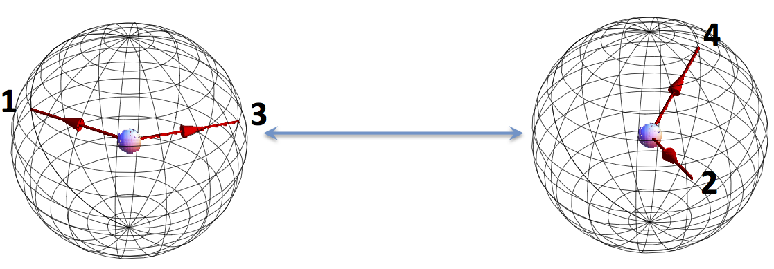
Figure 2: A schematic representation of the EPR/Bohm experimental set up. Explanations in the text.

In the form of a content-context matrix the system can be presented as

$$\begin{array}[]{|c|c|c|c||c|}\hline\cr R_{1}^{1}&R_{2}^{1}&&&c^{1}\\ \hline\cr&R_{2}^{2}&R_{3}^{2}&&c^{2}\\ \hline\cr&&R_{3}^{3}&R_{4}^{3}&c^{3}\\ \hline\cr R_{1}^{4}&&&R_{4}^{4}&c^{4}\\ \hline\cr\hline\cr\begin{array}[]{c}q_{1}\\ \textnormal{(Zora's 1)}\end{array}&\begin{array}[]{c}q_{2}\\ \textnormal{(Nico's 2)}\end{array}&\begin{array}[]{c}q_{3}\\ \textnormal{(Zora's 3)}\end{array}&\begin{array}[]{c}q_{4}\\ \textnormal{(Nico's 4)}\end{array}&\mathcal{C}_{4(a)}\\ \hline\cr\end{array}\>.$$ (14)

The measurements by Zora and Nico are made simultaneously, or at least close enough in time so that no signal about Zora’s choice of a direction can reach Nico before he makes his measurement, and vice versa. Because of this, the system is consistently connected,

$$R_{i}^{j}\overset{dist}{=}R_{i}^{j^{\prime}}$$

for any content $q_{i}$ and two contexts $c^{j}$ and $c^{j^{\prime}}$ in which $q_{i}$ is measured. Following the logic of contextuality analysis, we first establish that (because of the consistent connectedness)

$$\delta\left(R_{1}^{1},R_{1}^{4}\right)=\delta\left(R_{2}^{1},R_{2}^{2}\right)=\delta\left(R_{3}^{2},R_{3}^{3}\right)=\delta\left(R_{4}^{3},R_{4}^{4}\right)=0.$$

Then we compute

$$\delta\left(\left(R_{1}^{1},R_{1}^{4}\right),\left(R_{2}^{1},R_{2}^{2}\right),\left(R_{3}^{2},R_{3}^{3}\right),\left(R_{4}^{3},R_{4}^{4}\right)\right)\\ \\ =\min_{\begin{array}[]{c}\textnormal{all couplings}\\ \begin{array}[]{c}\left(S_{1}^{1},S_{4}^{1},S_{1}^{2},S_{2}^{2},S_{2}^{3},S_{3}^{3},S_{3}^{4},S_{4}^{4}\right)\\ \textnormal{ of system }\mathcal{C}_{4(a)}\end{array}\end{array}\textnormal{ }}\left(\Pr\left[S_{1}^{1}\not=S_{1}^{4}\right]+\Pr\left[S_{2}^{1}\not=S_{2}^{2}\right]+\Pr\left[S_{3}^{2}\not=S_{3}^{3}\right]+\Pr\left[S_{4}^{3}\not=S_{4}^{4}\right]\right).$$

The system is noncontextual if and only if this quantity is zero. As it turns out (and this is what was established by John Bell in his celebrated papers in the 1960s, [1, 2]), the directions $1,2,3,4$ can be chosen so that, by the laws of quantum mechanics, this quantity is greater than zero, making the system contextual.

In psychology, systems of the same $\mathcal{C}_{4}$-type have been of interest as representing the following empirical situation [23, 13, 16, 17, 11, 12, 15, 18]. Consider two variables having two values each, that can be manipulated in an experiment. Think, e.g., of a briefly presented visual object that can have one of two colors (red or green) and one of two shapes (square or oval), combined in the $2\times 2$ ways. In the experiment, an observer responds to the object by answering two Yes-No questions: “is the object red?” and “is the object square?”. If we simply identify these questions with contents, the resulting system of random variables looks like this:

$$\begin{array}[]{|c|c||l|}\hline\cr R_{1}^{1}&R_{2}^{1}&c^{1}:\textnormal{red and oval}\\ \hline\cr R_{1}^{2}&R_{2}^{2}&c^{2}:\textnormal{green and oval}\\ \hline\cr R_{1}^{3}&R_{2}^{3}&c^{3}:\textnormal{red and square}\\ \hline\cr R_{1}^{4}&R_{2}^{4}&c^{4}:\textnormal{green and square}\\ \hline\cr\hline\cr q_{1}:\textnormal{red?}&q_{2}:\textnormal{square?}&\mathcal{R}\\ \hline\cr\end{array}\>,$$ (15)

with the contexts describing the object being presented, and the contents the questions asked.

Although possible, this is not, however, an especially interesting way of conceptualizing the situation. It is more informative to describe the contents of the random variables as color and shape responses to the color and shape of the visual stimuli, respectively:

$$\begin{array}[]{|l|}\hline\cr q_{1}:\textnormal{does this red object appear red?}\\ \hline\cr q_{2}:\textnormal{does this square object appear square?}\\ \hline\cr q_{3}:\textnormal{does this green object appear red?}\\ \hline\cr q_{4}:\textnormal{does this oval object appear square?}\\ \hline\cr\end{array}$$

With the contexts remaining as they are in system (15), the experiment is now represented by a system of the $\mathcal{C}_{4}$-type:

$$\begin{array}[]{|c|c|c|c||c|}\hline\cr R_{1}^{1}&R_{2}^{1}&&&c^{1}\\ \hline\cr&R_{2}^{2}&R_{3}^{2}&&c^{2}\\ \hline\cr&&R_{3}^{3}&R_{4}^{3}&c^{3}\\ \hline\cr R_{1}^{4}&&&R_{4}^{4}&c^{4}\\ \hline\cr\hline\cr\begin{array}[]{c}q_{1}\\ \textnormal{(red)}\end{array}&\begin{array}[]{c}q_{2}\\ \textnormal{(square)}\end{array}&\begin{array}[]{c}q_{3}\\ \textnormal{(green)}\end{array}&\begin{array}[]{c}q_{4}\\ \textnormal{(oval)}\end{array}&\mathcal{C}_{4(b)}\\ \hline\cr\end{array}$$

Compared to system $\mathcal{C}_{4(c)}$ in (14), the physical situation described by $\mathcal{C}_{4(b)}$ is, of course, very different: e.g., instead of $R_{1}^{j}$ and $R_{3}^{j}$ being outcomes of spin measurements by Zora along two different directions, these random variables represent now responses to the color question when the color is red and when it is green, respectively. However, the logic of the contextuality analysis does not change. If this system turns out to be consistently connected and noncontextual, the interpretation of this in psychology is that the judgment of color is selectively influenced by object’s color (irrespective of its shape), and the judgment of shape is selectively influenced by object’s shape (irrespective of its color). Deviations from this pattern of selective influences, whether in the form of inconsistent connectedness or contextuality, or both, provide an interesting way of classifying (and quantifying) the ways object’s color may influence one’s judgment of its shape and vice versa.

7 What if the system is deterministic?

A deterministic quantity $r$ is a special case of a random variable: it is a random variable $R$ that attains the value $r$ with probability 1:

$$\Pr\left[R=r\right]=1.$$

It is convenient to present this as

$$R\equiv r.$$

A deterministic system is one containing only deterministic variables. For instance,

$$\begin{array}[]{|c|c|c|c|c||cc|}\hline\cr r_{1}^{1}&r_{2}^{1}&&r_{4}^{1}&&&c^{1}\\ \hline\cr r_{1}^{2}&&r_{3}^{2}&&&&c^{2}\\ \hline\cr&r_{2}^{3}&r_{3}^{3}&r_{4}^{3}&r_{5}^{3}&&c^{3}\\ \hline\cr&&r_{3}^{4}&&r_{5}^{4}&&c^{4}\\ \hline\cr\hline\cr&&&&&&\\ q_{1}&q_{2}&q_{3}&q_{4}&q_{5}&&\mathcal{D}\\ \hline\cr\end{array}$$ (16)

is a deterministic systems in which $r_{i}^{j}$ represents a random variable $R_{i}^{j}\equiv r_{i}^{j}$. The system can be consistently connected (if the value of $r_{i}^{j}$ does not depend on $j$) or inconsistently connected (otherwise).

It is easy to see, however, that a deterministic system is always noncontextual. Indeed, any two content-sharing $R_{i}^{j}\equiv r_{i}^{j}$ and $R_{i}^{j^{\prime}}\equiv r_{i}^{j^{\prime}}$ in this system have a single coupling ($S_{i}^{j}\equiv r_{i}^{j}$,$S_{i}^{j}\equiv r_{i}^{j}$), consisting of the same deterministic quantities but considered jointly distributed. It follows that

$$\delta\left(r_{i}^{j},r_{i}^{j^{\prime}}\right)=\left\{\begin{array}[]{ccc}1&\textnormal{if}&r_{i}^{j}\not=r_{i}^{j^{\prime}}\\ 0&\textnormal{if}&r_{i}^{j}=r_{i}^{j^{\prime}}\end{array}\right..$$

The entire deterministic system in (16) also has a single coupling, one containing the same deterministic quantities as the system itself, but considered jointly distributed. Clearly, the subcoupling $\left(S_{i}^{j}\equiv r_{i}^{j},S_{i}^{j^{\prime}}\equiv r_{i}^{j^{\prime}}\right)$ extracted from this coupling is precisely the same as the coupling of $R_{i}^{j}\equiv r_{i}^{j}$ and $R_{i}^{j^{\prime}}\equiv r_{i}^{j^{\prime}}$ taken in isolation, and

$$\delta\left(\left\{\left(r_{i}^{j},r_{i}^{j^{\prime}}\right):\textnormal{all such pairs}\right\}\right)=\sum_{\textnormal{all such pairs}}\delta\left(r_{i}^{j},r_{i}^{j^{\prime}}\right).$$

One might conclude that deterministic systems are of no interest for contextuality analysis. This is not always true, however. There are cases when we know that a system is deterministic, but we do not know which of a set of possible deterministic systems it is, because it can be any of them. Let us look at this in detail, using as examples systems consisting of logical truth values of various statements.

Consider first the following $\mathcal{C}_{4}$-type system:

$$\begin{array}[]{|c|c|c|c||c|}\hline\cr R_{1}^{1}\equiv+1&R_{2}^{1}\equiv-1&&&c^{1}\\ \hline\cr&R_{2}^{2}\equiv+1&R_{3}^{2}\equiv-1&&c^{2}\\ \hline\cr&&R_{3}^{3}\equiv+1&R_{4}^{3}\equiv-1&c^{3}\\ \hline\cr R_{1}^{4}\equiv-1&&&R_{4}^{4}\equiv+1&c^{4}\\ \hline\cr\hline\cr q_{1}&q_{2}&q_{3}&q_{4}&\mathcal{C}_{4(c)}\\ \hline\cr\end{array}\>,$$ (17)

where $+1$ and $-1$ encode truth values (true and false), and the contents are the statements

$$\begin{array}[]{|l|c|}\hline\cr q_{1}:\textnormal{"my name is Zora"}&q_{2}:\textnormal{"my name is Nico"}\\ \hline\cr q_{3}:\textnormal{"my name is Max"}&q_{4}:\textnormal{"my name is Alex"}\\ \hline\cr\end{array}\>.$$

Equivalently, the contents could also be formulated as questions, “is my name Zora?” and “is my name Nico?”, in which case $+1$ and $-1$ would encode answers Yes and No. In the following, however, I will refer to the $q$’s as statements, and the values of the variables as truth values. The contexts justifying the truth values in (17) are

$$\begin{array}[]{|l|c|}\hline\cr c^{1}:\textnormal{the statements are made by Zora}&c^{2}:\textnormal{the statements are made by Nico}\\ \hline\cr c^{3}:\textnormal{the statements are made by Max}&c^{4}:\textnormal{the statements are made by Alex}\\ \hline\cr\end{array}\>.$$

This is a situation when the truth values are determined uniquely, the system is deterministic, and consequently it is noncontextual (even though context-dependence in it is salient in the form of inconsistent connectedness).

Consider next another system of the $C_{4}$-type,

$$\begin{array}[]{|c|c|c|c||c|}\hline\cr R_{1}^{1}&R_{2}^{1}&&&c^{1}\\ \hline\cr&R_{2}^{2}&R_{3}^{2}&&c^{2}\\ \hline\cr&&R_{3}^{3}&R_{4}^{3}&c^{3}\\ \hline\cr R_{1}^{4}&&&R_{4}^{4}&c^{4}\\ \hline\cr\hline\cr q_{1}:\textnormal{"}q_{2}\textnormal{ is true"}&q_{2}:\textnormal{"}q_{3}\textnormal{ is true"}&q_{3}:\textnormal{"}q_{4}\textnormal{ is true"}&q_{4}:\textnormal{"}q_{1}\textnormal{ is false"}&\mathcal{C}_{4(d)}\\ \hline\cr\end{array}\>,$$

with contents/statements of a very different kind, and the contexts which here (at least provisionally) can simply be defined by which statements they include: $c^{1}$ includes $\left(q_{1},q_{2}\right)$, $c^{2}$ includes $\left(q_{2},q_{3}\right)$, etc.

One can recognize here a formalization of the quadripartite version of the Liar antinomy: one can begin with any statement, say $q_{3}$, assume it is true, conclude that then $q_{4}$ is true, then $q_{1}$ is false, then $q_{2}$ is false, and then $q_{3}$ is false; and if one assumes that $q_{3}$ is false, then by the analogous chain of assignments one arrives to $q_{3}$ being true. There is no consistent assignment of truth values in this system. In the language of CbD, the truth values of the statements in $\mathcal{C}_{4(d)}$ can only be described by an inconsistently connected deterministic system.

We come to the main issue now: $\mathcal{C}_{4(d)}$ is certainly a deterministic system (because truth values of statements within a context are fixed), but which deterministic system is it? There are 16 possible ways of filling this system with truth values:

$$\begin{array}[]{c}\begin{array}[]{|c|c|c|c|}\hline\cr+1&+1&&\\ \hline\cr&+1&+1&\\ \hline\cr&&+1&+1\\ \hline\cr-1&&&+1\\ \hline\cr\end{array}\>,\quad\begin{array}[]{|c|c|c|c|}\hline\cr+1&+1&&\\ \hline\cr&+1&+1&\\ \hline\cr&&-1&-1\\ \hline\cr+1&&&-1\\ \hline\cr\end{array}\>,\\ \\ \begin{array}[]{|c|c|c|c|}\hline\cr+1&+1&&\\ \hline\cr&-1&-1&\\ \hline\cr&&+1&+1\\ \hline\cr-1&&&+1\\ \hline\cr\end{array}\>,\quad\begin{array}[]{|c|c|c|c|}\hline\cr+1&+1&&\\ \hline\cr&+1&+1&\\ \hline\cr&&-1&-1\\ \hline\cr+1&&&-1\\ \hline\cr\end{array},\\ \textnormal{etc.}\end{array}$$

The only constraint in generating these systems is that

1. in the first three contexts (rows) the truth values of the two variables coincide (because the first statement in them says that the second one is true, and the second one does not refer to the first one);

2. in context $c^{4}$ (the last row) the truth values of the two variables are opposite (because $q_{4}$ says that $q_{1}$ is false, and $q_{1}$ does not refer to $q_{4}$).

We see that although random variability in $\mathcal{C}_{4(d)}$ is absent, we have in its place epistemic uncertainty. This opens the possibility of attaching epistemic (Bayesian) probabilities to the 16 possible deterministic variants of $\mathcal{C}_{4(d)}$, and obtaining as a result a system of epistemic random variables. Mathematically, such a variable is treated in precisely the same way as an ordinary (“frequentist”) random variable. For instance, we can say that an epistemic variable $R$ can have values $+1$ and $-1$ with Bayesian probabilities $p$ and $1-p$. This means that $R$ in fact is a deterministic quantity that can be either $+1$ or $-1$, and the degree of rational belief that $R$ is $+1$ (given what we know of it) is $p$. In all computational respects, however, $R$ is treated as if it was a variable that sometimes can be $+1$ and sometimes $-1$.

If we choose equal weights for all 16 deterministic variants of $\mathcal{C}_{4(d)}$ (simply because we have no rational grounds for preferring some of them to others), the resulting system will have the following Bayesian distributions:

$$\begin{array}[]{c|c|c|c}\begin{array}[]{c}\textnormal{context }c^{i},\\ i=1,2,3\end{array}&R_{i+1}^{i}=+1&R_{i+1}^{i}=-1\\ \hline\cr R_{i}^{i}=+1&\nicefrac{{1}}{{2}}&0&\nicefrac{{1}}{{2}}\\ \hline\cr R_{i}^{i}=-1&0&\nicefrac{{1}}{{2}}&\nicefrac{{1}}{{2}}\\ \hline\cr&\nicefrac{{1}}{{2}}&\nicefrac{{1}}{{2}}\end{array}$$ (18)

and

$$\begin{array}[]{c|c|c|c}\textnormal{context }c^{4}&R_{1}^{4}=+1&R_{1}^{4}=-1\\ \hline\cr R_{4}^{4}=+1&0&\nicefrac{{1}}{{2}}&\nicefrac{{1}}{{2}}\\ \hline\cr R_{4}^{4}=-1&\nicefrac{{1}}{{2}}&0&\nicefrac{{1}}{{2}}\\ \hline\cr&\nicefrac{{1}}{{2}}&\nicefrac{{1}}{{2}}\end{array}\>.$$ (19)

This system is clearly contextual. Indeed, since it is consistently connected,

$$\delta\left(R_{1}^{1},R_{1}^{4}\right)=\delta\left(R_{2}^{1},R_{2}^{2}\right)=\delta\left(R_{3}^{2},R_{3}^{3}\right)=\delta\left(R_{4}^{3},R_{4}^{4}\right)=0.$$ (20)

At the same time,

$$\delta\left(\left(R_{1}^{1},R_{1}^{4}\right),\left(R_{2}^{1},R_{2}^{2}\right),\left(R_{3}^{2},R_{3}^{3}\right),\left(R_{4}^{3},R_{4}^{4}\right)\right)\\ \\ =\min_{\begin{array}[]{c}\textnormal{all couplings}\\ \begin{array}[]{c}\left(S_{1}^{1},S_{4}^{1},S_{1}^{2},S_{2}^{2},S_{2}^{3},S_{3}^{3},S_{3}^{4},S_{4}^{4}\right)\\ \textnormal{ of system }\mathcal{C}_{4(d)}\end{array}\end{array}\textnormal{ }}\left(\Pr\left[S_{1}^{1}\not=S_{1}^{4}\right]+\Pr\left[S_{2}^{1}\not=S_{2}^{2}\right]+\Pr\left[S_{3}^{2}\not=S_{3}^{3}\right]+\Pr\left[S_{4}^{3}\not=S_{4}^{4}\right]\right)>0.$$ (21)

This is easy to see. This quantity could be zero only if, in some coupling of $\mathcal{C}_{4(a)}$, the equalities in the first row below all held with probability 1:

$$\lx@xy@svg{\hbox{\raise 0.0pt\hbox{\kern 17.78607pt\hbox{\ignorespaces\ignorespaces\ignorespaces\hbox{\vtop{\kern 0.0pt\offinterlineskip\halign{\entry@#!@&&\entry@@#!@\cr&&&\\&&&\crcr}}}\ignorespaces{\hbox{\kern-17.78607pt\raise 0.0pt\hbox{\hbox{\kern 0.0pt\raise 0.0pt\hbox{\hbox{\kern 3.0pt\raise 0.0pt\hbox{$\textstyle{S_{1}^{4}=S_{1}^{1}\ignorespaces\ignorespaces\ignorespaces\ignorespaces}$}}}}}}}\ignorespaces\ignorespaces\ignorespaces\ignorespaces{}{\hbox{\lx@xy@droprule}}\ignorespaces{\hbox{\kern 0.0pt\raise-28.90222pt\hbox{\hbox{\kern 0.0pt\raise 0.0pt\hbox{\lx@xy@tip{1}\lx@xy@tip{-1}}}}}}{\hbox{\lx@xy@droprule}}{\hbox{\lx@xy@droprule}}{\hbox{\kern 46.23882pt\raise 0.0pt\hbox{\hbox{\kern 0.0pt\raise 0.0pt\hbox{\hbox{\kern 3.0pt\raise 0.0pt\hbox{$\textstyle{S_{2}^{1}=S_{2}^{2}\ignorespaces\ignorespaces\ignorespaces\ignorespaces}$}}}}}}}\ignorespaces\ignorespaces\ignorespaces\ignorespaces{}{\hbox{\lx@xy@droprule}}\ignorespaces{\hbox{\kern 64.02489pt\raise-28.90222pt\hbox{\hbox{\kern 0.0pt\raise 0.0pt\hbox{\lx@xy@tip{1}\lx@xy@tip{-1}}}}}}{\hbox{\lx@xy@droprule}}{\hbox{\lx@xy@droprule}}{\hbox{\kern 110.2637pt\raise 0.0pt\hbox{\hbox{\kern 0.0pt\raise 0.0pt\hbox{\hbox{\kern 3.0pt\raise 0.0pt\hbox{$\textstyle{S_{3}^{2}=S_{3}^{3}\ignorespaces\ignorespaces\ignorespaces\ignorespaces}$}}}}}}}\ignorespaces\ignorespaces\ignorespaces\ignorespaces{}{\hbox{\lx@xy@droprule}}\ignorespaces{\hbox{\kern 128.04977pt\raise-28.90222pt\hbox{\hbox{\kern 0.0pt\raise 0.0pt\hbox{\lx@xy@tip{1}\lx@xy@tip{-1}}}}}}{\hbox{\lx@xy@droprule}}{\hbox{\lx@xy@droprule}}{\hbox{\kern 179.42744pt\raise 0.0pt\hbox{\hbox{\kern 0.0pt\raise 0.0pt\hbox{\hbox{\kern 3.0pt\raise 0.0pt\hbox{$\textstyle{S_{4}^{3}=S_{4}^{4}\ignorespaces\ignorespaces\ignorespaces\ignorespaces}$}}}}}}}\ignorespaces\ignorespaces\ignorespaces\ignorespaces{}{\hbox{\lx@xy@droprule}}\ignorespaces{\hbox{\kern 197.21352pt\raise-28.90222pt\hbox{\hbox{\kern 0.0pt\raise 0.0pt\hbox{\lx@xy@tip{1}\lx@xy@tip{-1}}}}}}{\hbox{\lx@xy@droprule}}{\hbox{\lx@xy@droprule}}{\hbox{\kern-17.78607pt\raise-40.53998pt\hbox{\hbox{\kern 0.0pt\raise 0.0pt\hbox{\hbox{\kern 3.0pt\raise 0.0pt\hbox{$\textstyle{S_{1}^{1}=S_{2}^{1}\ignorespaces\ignorespaces\ignorespaces\ignorespaces}$}}}}}}}\ignorespaces\ignorespaces\ignorespaces{}\ignorespaces\ignorespaces{\hbox{\lx@xy@drawline@}}\ignorespaces{\hbox{\kern 56.43819pt\raise-4.80444pt\hbox{\hbox{\kern 0.0pt\raise 0.0pt\hbox{\lx@xy@tip{1}\lx@xy@tip{-1}}}}}}\ignorespaces\ignorespaces{\hbox{\lx@xy@drawline@}}\ignorespaces{\hbox{\lx@xy@drawline@}}{\hbox{\kern 46.23882pt\raise-40.53998pt\hbox{\hbox{\kern 0.0pt\raise 0.0pt\hbox{\hbox{\kern 3.0pt\raise 0.0pt\hbox{$\textstyle{S_{2}^{2}=S_{3}^{2}\ignorespaces\ignorespaces\ignorespaces\ignorespaces}$}}}}}}}\ignorespaces\ignorespaces\ignorespaces{}\ignorespaces\ignorespaces{\hbox{\lx@xy@drawline@}}\ignorespaces{\hbox{\kern 120.46307pt\raise-4.80444pt\hbox{\hbox{\kern 0.0pt\raise 0.0pt\hbox{\lx@xy@tip{1}\lx@xy@tip{-1}}}}}}\ignorespaces\ignorespaces{\hbox{\lx@xy@drawline@}}\ignorespaces{\hbox{\lx@xy@drawline@}}{\hbox{\kern 110.2637pt\raise-40.53998pt\hbox{\hbox{\kern 0.0pt\raise 0.0pt\hbox{\hbox{\kern 3.0pt\raise 0.0pt\hbox{$\textstyle{S_{3}^{3}=S_{4}^{3}\ignorespaces\ignorespaces\ignorespaces\ignorespaces}$}}}}}}}\ignorespaces\ignorespaces\ignorespaces{}\ignorespaces\ignorespaces{\hbox{\lx@xy@drawline@}}\ignorespaces{\hbox{\kern 189.01688pt\raise-4.80444pt\hbox{\hbox{\kern 0.0pt\raise 0.0pt\hbox{\lx@xy@tip{1}\lx@xy@tip{-1}}}}}}\ignorespaces\ignorespaces{\hbox{\lx@xy@drawline@}}\ignorespaces{\hbox{\lx@xy@drawline@}}{\hbox{\kern 174.28859pt\raise-40.53998pt\hbox{\hbox{\kern 0.0pt\raise 0.0pt\hbox{\hbox{\kern 3.0pt\raise 0.0pt\hbox{$\textstyle{S_{4}^{4}\not=S_{1}^{4}}$}}}}}}}\ignorespaces}}}}\ignorespaces\>. \textstyle{S_{1}^{4}=S_{1}^{1}\ignorespaces\ignorespaces\ignorespaces\ignorespaces} \textstyle{S_{2}^{1}=S_{2}^{2}\ignorespaces\ignorespaces\ignorespaces\ignorespaces} \textstyle{S_{3}^{2}=S_{3}^{3}\ignorespaces\ignorespaces\ignorespaces\ignorespaces} \textstyle{S_{4}^{3}=S_{4}^{4}\ignorespaces\ignorespaces\ignorespaces\ignorespaces} \textstyle{S_{1}^{1}=S_{2}^{1}\ignorespaces\ignorespaces\ignorespaces\ignorespaces} \textstyle{S_{2}^{2}=S_{3}^{2}\ignorespaces\ignorespaces\ignorespaces\ignorespaces} \textstyle{S_{3}^{3}=S_{4}^{3}\ignorespaces\ignorespaces\ignorespaces\ignorespaces} \textstyle{S_{4}^{4}\not=S_{1}^{4}} \textstyle{S_{1}^{4}=S_{1}^{1}\ignorespaces\ignorespaces\ignorespaces\ignorespaces} \textstyle{S_{2}^{1}=S_{2}^{2}\ignorespaces\ignorespaces\ignorespaces\ignorespaces} \textstyle{S_{3}^{2}=S_{3}^{3}\ignorespaces\ignorespaces\ignorespaces\ignorespaces} \textstyle{S_{4}^{3}=S_{4}^{4}\ignorespaces\ignorespaces\ignorespaces\ignorespaces} \textstyle{S_{1}^{1}=S_{2}^{1}\ignorespaces\ignorespaces\ignorespaces\ignorespaces} \textstyle{S_{2}^{2}=S_{3}^{2}\ignorespaces\ignorespaces\ignorespaces\ignorespaces} \textstyle{S_{3}^{3}=S_{4}^{3}\ignorespaces\ignorespaces\ignorespaces\ignorespaces} \textstyle{S_{4}^{4}\not=S_{1}^{4}}$$

But in any coupling of $\mathcal{C}_{4(a)}$, the equalities in the second row also hold with probability 1, because they copy (18) and (19). Reading now all the equalities above from left to right along the arrows as a chain

$$S_{1}^{4}=S_{1}^{1}=S_{2}^{1}=S_{2}^{2}=\ldots,$$

one arrives at a contradiction

$$S_{1}^{4}\not=S_{1}^{4}.$$

In essence, this is the same reasoning as that establishing the unremovable contraction in the Liar antinomy. However, this time it merely serves the purpose of establishing that our system is contextual. In fact, the degree of contextuality here, computed as the difference between (21) and the (zero) sum of the deltas in (20), is maximal among all possible systems of the $\mathcal{C}_{4}$-type.

$\begin{array}[]{c}\begin{array}[]{|c|c|c|c||c|}\hline\cr R_{1}^{1}&R_{2}^{1}&&&c^{1}\\ \hline\cr&R_{2}^{2}&R_{3}^{2}&&c^{2}\\ \hline\cr&&R_{3}^{3}&R_{4}^{3}&c^{3}\\ \hline\cr R_{1}^{4}&&&R_{4}^{4}&c^{4}\\ \hline\cr R_{1}^{5}&R_{1}^{5}&R_{1}^{5}&R_{1}^{5}&c^{5}\\ \hline\cr\hline\cr q_{1}&q_{2}&q_{3}&q_{4}&\mathcal{E}\\ \hline\cr\end{array}\end{array}$

Figure 3: “Ascending-Descending” by M. C. Escher. The four flights of stairs are enumerated $q_{1},q_{2},q_{3},q_{4}$. The epistemic random variables have values ascending and descending, and in each of the the first four contexts they are perfectly correlated. The fifth context is a mixture of the quadruples of values precisely two of which are ascending (so that travelers always end up in the same place from where they started). The resulting epistemic system is contextual [55].

We could use other multipartite versions of the Liar paradox, with three or five or any number of statements, all leading to the same outcome. A special mention is needed of the bipartite version. In this system it is no longer possible to define the contexts simply by the contents of the variables they include. Instead we once again need to use the order of the contents, this time interpreted as the direction of inference: $q\rightarrow q^{\prime}$ means that we assign truth values to $q$ and infer the corresponding truth values for $q^{\prime}$. The resulting system is

$$\begin{array}[]{|c|c||c|}\hline\cr R_{1}^{1}&R_{2}^{1}&c^{1}:q_{1}\rightarrow q_{2}\\ \hline\cr R_{1}^{2}&R_{2}^{2}&c^{2}:q_{2}\rightarrow q_{1}\\ \hline\cr\hline\cr q_{1}=\textnormal{"}q_{2}\textnormal{ is true"}&q_{2}:\textnormal{"}q_{1}\textnormal{ is false"}&\mathcal{C}_{2(d)}\\ \hline\cr\end{array}\>,$$

with four possible deterministic variants:

$$\begin{array}[]{c}\begin{array}[]{|c|c|}\hline\cr+1&+1\\ \hline\cr-1&+1\\ \hline\cr\end{array}\>,\quad\begin{array}[]{|c|c|}\hline\cr+1&+1\\ \hline\cr+1&-1\\ \hline\cr\end{array}\>,\\ \\ \begin{array}[]{|c|c|}\hline\cr-1&-1\\ \hline\cr-1&+1\\ \hline\cr\end{array}\>,\quad\begin{array}[]{|c|c|}\hline\cr+1&+1\\ \hline\cr+1&-1\\ \hline\cr\end{array}\>.\end{array}$$

Mixing them with equal epistemic probabilities creates a consistently connected and highly contextual system (maximally contextual among all cyclic systems of rank 2).

Logical paradoxes are not, of course, the only application of contextuality analysis with epistemic random variables. It seems that many “strange” or “paradoxical” situations can be converted into contextual epistemic systems [55, 57]. Among other applications are such objects as the Penroses’ “impossible figures” and M. C. Escher’s pictures (as in Figure 3).

8 The right to ignore (or not to)

I will mention now some aspects of the Contextuality-by-Default theory (CbD) that seem to pose difficulties for understanding. Questions about them are being asked often and in spite of having been repeatedly addressed in published literature.

The most basic aspect of CbD is double indexation of the random variables. The response to a given question $q$ is a random variable $R_{q}^{c}$ whose identity is determined not only by $q$ but also by the context $c$ in which $q$ is responded to. This looks innocuous enough, but it puzzles some when a system being analyzed is consistently connected, i.e. when changing $c$ in $R_{q}^{c}$ does not change the distribution. And the puzzlement may increase when our knowledge tells us there is no possible way in which different contexts $c$ can differently influence the random variables $R_{q}^{c}$.

Consider again the system $\mathcal{C}_{4(a)}$ in (14), from which we date contextuality studies. I reproduce it here for the reader’s convenience:

$$\begin{array}[]{|c|c|c|c||c|}\hline\cr R_{1}^{1}&R_{2}^{1}&&&c^{1}\\ \hline\cr&R_{2}^{2}&R_{3}^{2}&&c^{2}\\ \hline\cr&&R_{3}^{3}&R_{4}^{3}&c^{3}\\ \hline\cr R_{1}^{4}&&&R_{4}^{4}&c^{4}\\ \hline\cr\hline\cr\begin{array}[]{c}q_{1}\\ \textnormal{(Zora's 1)}\end{array}&\begin{array}[]{c}q_{2}\\ \textnormal{(Nico's 2)}\end{array}&\begin{array}[]{c}q_{3}\\ \textnormal{(Zora's 3)}\end{array}&\begin{array}[]{c}q_{4}\\ \textnormal{(Nico's 4)}\end{array}&\mathcal{C}_{4(a)}\\ \hline\cr\end{array}\>.$$

In this system, Nico’s choice between directions 2 and $4$ can in no ways affect Zora’s measurements of spin along direction $1$. Nevertheless, when Nico switches from direction $2$ to $4$, the random variable describing the outcome of Zora’s measurement of spin along direction $1$ ceases to be $R_{1}^{1}$ and becomes $R_{1}^{4}$. It looks like Nico has influenced Zora’s measurements after all. Isn’t it an example of what Albert Einstein famously called a “spooky action at a distance”?

The answer is, it is not. Nico’s choices are undetectable by Zora. Whether he chooses direction 2 or direction 4, Zora can see no changes in the statistical properties of what she observes when she measures spins along direction 1. “Action” means information transmitted, and no information is transmitted from Nico to Zora (and vice versa). The fact that in at least one of the pairs

$$\left\{R_{1}^{1},R_{1}^{4}\right\},\left\{R_{2}^{1},R_{2}^{2}\right\},\left\{R_{3}^{3},R_{3}^{4}\right\},\left\{R_{4}^{3},R_{4}^{4}\right\}$$

the two random variables cannot be viewed as being the same can be established by neither Zora nor Nico. It can only be established by a Max who receives the choice of directions and outcomes of measurements from both Zora and Nico and computes the joint distributions in contexts $c^{1},c^{2},c^{3},c^{4}$.

An important point here is that compared to Max, Zora does not misunderstand or miss anything when she sees no difference between $R_{1}^{1}$ and $R_{1}^{4}$ or between $R_{3}^{3}$ and $R_{3}^{4}$. Her understanding is no less complete or less correct. Zora and Max simply deal with different systems of random variables. In the same way Max’s understanding is no less complete or less correct than that of an Alex who, in addition to knowing what Max knows, observes whether solar activity during the measurements is high or low. In Alex’s system, each context of system $\mathcal{C}_{4(a)}$ is split into two contexts, e.g., $c^{1}$ is replaced with

$$\begin{array}[]{|c|c|c|c||c|}\hline\cr R_{1}^{1,high}&R_{2}^{1,high}&&&c^{1,high}\\ \hline\cr R_{1}^{1,low}&R_{2}^{1,low}&&&c^{1,low}\\ \hline\cr\hline\cr q_{1}&q_{2}&q_{3}&q_{4}&\mathcal{C}_{4(a)}/c^{1}\textnormal{ only}\\ \hline\cr\end{array}\>.$$

In studying a system of random variable one always can ignore any of the circumstances that do not affect the distributions of the variables. Or one can choose not to ignore such circumstances, to systematically record them and make them part of the contexts. If a circumstance is irrelevant (as it may be in the case of Alex’s recording of solar activity), one will find this out by considering couplings of the system. Thus, one may establish that the contextuality analysis of the system does not change if all couplings are constrained by

$$\Pr\left[S_{i}^{j,high}=S_{i}^{j,low}\right]=1,$$

for any $R_{i}^{j}$ in the original system $\mathcal{C}_{4(a)}$. This would mean that $R_{i}^{j,high}$ and $R_{i}^{j,low}$ can be viewed as being one and the same random variable (assuming, of course, that solar activity is indeed irrelevant).

This reasoning fully applies to the issue often raised by those who enjoy shallow paradoxes. If one records values of a random variable $R$ in, say, chronological order, and simultaneously records the ordinal positions of these values in the sequence (as part of their contexts),

$$\begin{array}[]{|c|c|c|c|c|}\hline\cr r_{1}&r_{2}&\ldots&r_{n}&\ldots\\ \hline\cr 1&2&\ldots&n&\ldots\\ \hline\cr\end{array}\>,$$

would not this transform all these realizations of a single random variable into pairwise stochastically unrelated random variables

$$R^{1},R^{2},\ldots,R^{n},\ldots$$

with a single realization each? The answer is yes, if one so wishes (one may also choose to ignore the ordinal positions of the observations altogether), but then a standard view is immediately restored when one considers couplings of these random variables. For instance, the iid coupling (corresponding to the standard statistical concept of independent identically distributed variables) has the structure

$$\begin{array}[]{cccccc}&R^{1}&R^{2}&\ldots&R^{n}&\ldots\\ S^{1}&\boxed{\overset{}{\>r_{1}^{1}=r_{1}}\>}&r_{2}^{1}&\ldots&r_{n}^{1}&\ldots\\ S^{2}&r_{1}^{2}&\boxed{\overset{}{\>r_{2}^{2}=r_{2}}\>}&\ldots&r_{n}^{2}&\ldots,\\ \vdots&\vdots&\vdots&\ddots&\vdots&\ddots\\ S^{n}&r_{1}^{n}&r_{2}^{n}&\ldots&\boxed{\overset{}{\>r_{n}^{n}=r_{n}}\>}&\ldots\\ \vdots&\vdots&\vdots&\ddots&\vdots&\ddots\end{array}$$

where the boxed values are those factually observed, whereas all other values are independently sampled from the distribution of $R$. More details are available in Refs. [37, 61].

Finally, does the double-indexation in CbD lend any support to the holistic view of the universe, the view that “everything depends on everything else”? The answer is that the opposite is true, CbD supports a radically analytic view. First, as we have established, unless distributions of two given content-sharing variables are found to be different (which is ubiquitous but not universal) one can ignore the difference between their contexts, i.e., disregard all other variables in these contexts. This will redefine the system, but will not be wrong. Second, the difference in the identity of two content-sharing variables in different contexts (whether their distributions are the same or not) involves no change in the colloquial meaning of the word. The notion of a change implies that something that preserves its identity (e.g., a moving body) changes some of its properties (e.g., position in space). However, $R_{2}^{1}$ and $R_{2}^{2}$ (having the same content in different contexts) are simply different random variables, stochastically unrelated because they occur in mutually exclusive contexts. The difference between them is precisely the same as that between $R_{2}^{1}$ and $R_{1}^{1}$ (different contents in the same context). By choosing a different question to ask, one switches to considering another random variable rather than “changes” the previous one. The same happens when one chooses a different context: one simply switches to considering a different random variable. If I see Max and then see Alex, it does not mean that Max has changed into Alex.

The core of these and other problems with understanding CbD, it seems to me, is in the tendency to view random variables as empirical objects. They are not. Random variables are our descriptions of empirical objects. They are part of our knowledge of the world, and the same as any other knowledge, they can appear, disappear, and be revised as soon as we adopt a new point of view or gain new evidence.

References

• [1] Bell, J. (1964). On the Einstein-Podolsky-Rosen paradox. Physics 1, 195-200.
• [2] Bell, J. (1966). On the problem of hidden variables in quantum mechanics. Review of Modern Physic 38:447-453.
• [3] Kochen, S., Specker, E. P. (1967). The problem of hidden variables in quantum mechanics. Journal of Mathematics and Mechanics 17:59–87.
• [4] Clauser, J.F. , Horne, M.A. , Shimony, A., & Holt, R.A. (1969). Proposed experiment to test local hidden-variable theories. Physical Review Letters 23:880-884.
• [5] Clauser, J.F., Horne, M.A. (1974). Experimental consequences of objective local theories. Physical Review D 10:526-535.
• [6] Fine, A. (1982). Joint distributions, quantum correlations, and commuting observables. Journal of Mathematical Physics 23:1306-1310.
• [7] Cabello, A., Estebaranz, J., & Garcìa-Alcaine, G. (1996). Bell-Kochen-Specker theorem: A proof with 18 vectors. Physics Letters A 212:183-187.
• [8] Cabello, A. (2008). Experimentally testable state-independent quantum contextuality. Physical Review Letters 101, 210401.
• [9] Klyachko, A.A., Can, M.A., Binicioglu, S., & Shumovsky, A.S. (2008). A simple test for hidden variables in spin-1 system. Physical Review Letters 101:020403.
• [10] Kurzynski, P., Cabello, A., & Kaszlikowski, D. (2014). Fundamental monogamy relation between contextuality and nonlocality. Physical Review Letters 112:100401.
• [11] Sternberg, S. (1969). The discovery of processing stages: Extensions of Donders’ method. In W.G. Koster (Ed.), Attention and Performance II. Acta Psychologica 30:276–315.
• [12] Townsend, J. T. (1984). Uncovering mental processes with factorial experiments. Journal of Mathematical Psychology, 28, 363–400.
• [13] Dzhafarov, E.N. (2003). Selective influence through conditional independence. Psychometrika, 68:7-26.
• [14] Dzhafarov, E.N., & Gluhovsky, I. (2006). Notes on selective influence, probabilistic causality, and probabilistic dimensionality. Journal of Mathematical Psychology, 50:390-401.
• [15] Kujala, J.V., Dzhafarov, E.N. (2008). Testing for selectivity in the dependence of random variables on external factors. Journal of Mathematical Psychology 52:128–144.
• [16] Dzhafarov, E.N., Kujala, J.V. (2010). The joint distribution criterion and the distance tests for selective probabilistic causality. Frontiers in Psychology: Quantitative Psychology and Measurement 1:151 doi: 10.3389/fpsyg.2010.0015.
• [17] Dzhafarov, E.N., & Kujala, J.V. (2016). Probability, random variables, and selectivity. In W.Batchelder, H. Colonius, E.N. Dzhafarov, J. Myung (Eds), The New Handbook of Mathematical Psychology (pp. 85-150). Cambridge University Press.
• [18] Zhang, R. Dzhafarov, E.N. (2015). Noncontextuality with marginal selectivity in reconstructing mental architectures. Frontiers in Psychology: Cognition 1:12 doi: 10.3389/fpsyg.2015.00735.
• [19] Dzhafarov, E.N. & Kujala, J.V. (2012). Selectivity in probabilistic causality: Where psychology runs into quantum physics. Journal of Mathematical Psychology 56, 54-63.
• [20] Dzhafarov, E.N., Kujala, J.V. (2012). Quantum entanglement and the issue of selective influences in psychology: An overview. Lecture Notes in Computer Science 7620:184-195.
• [21] Dzhafarov, E.N., Kujala, J.V. (2013). All-possible-couplings approach to measuring probabilistic context. PLoS ONE 8(5):e61712. doi:10.1371/journal.pone.0061712.
• [22] Dzhafarov, E.N., Kujala, J.V. (2013). Order-distance and other metric-like functions on jointly distributed random variables. Proceedings of the American Mathematical Society 141:3291-3301.
• [23] Dzhafarov, E.N., Kujala, J.V. (2014). Selective influences, marginal selectivity, and Bell/CHSH inequalities. Topics in Cognitive Science, 6, 121–128.
• [24] Dzhafarov, E.N., Kujala, J.V. (2014). A qualified Kolmogorovian account of probabilistic contextuality. Lecture Notes in Computer Science 8369:201-212.
• [25] Dzhafarov, E.N., Kujala, J.V. (2014). Contextuality is about identity of random variables. Physica Scripta T163:014009.
• [26] Dzhafarov, E.N., Kujala, J.V. (2015). Conversations on contextuality. In E.N. Dzhafarov, S. Jordan, R. Zhang, V. Cervantes (Eds). Contextuality from Quantum Physics to Psychology (pp. 1-22). New Jersey: World Scientific.
• [27] Kujala, J.V., & Dzhafarov, E.N. (2015). Probabilistic Contextuality in EPR/Bohm-type systems with signaling allowed. In E.N. Dzhafarov, S. Jordan, R. Zhang, V. Cervantes (Eds). Contextuality from Quantum Physics to Psychology (pp. 287-308). New Jersey: World Scientific.
• [28] Bacciagaluppi, G. (2015). Einsten, Bohm, and Leggett-Garg. In E.N. Dzhafarov, S. Jordan, R. Zhang, V. Cervantes (Eds). Contextuality from Quantum Physics to Psychology (pp. 63-76). New Jersey: World Scientific.
• [29] Dzhafarov, E.N., & Kujala, J.V., & Larsson, J.-Å. (2015). Contextuality in three types of quantum-mechanical systems. Foundations of Physics 7, 762-782.
• [30] Dzhafarov, E.N., Zhang, R., Kujala, J.V. (2015). Is there contextuality in behavioral and social systems? Philosophical Transactions of the Royal Society A 374:20150099.
• [31] Kujala, J.V., Dzhafarov, E.N., Larsson, J-Å (2015). Necessary and sufficient conditions for extended noncontextuality in a broad class of quantum mechanical systems. Physical Review Letters 115:150401.
• [32] Dzhafarov, E.N., Kujala, J.V., Cervantes, V.H., Zhang, R., Jones, M. (2016). On contextuality in behavioral data. Philosophical Transactions of the Royal Society A 374:20150234.
• [33] Dzhafarov, E.N., Kujala, J.V., & Cervantes, V.H. (2016). Contextuality-by-Default: A brief overview of ideas, concepts, and terminology. Lecture Notes in Computer Science 9535:12-23.
• [34] Dzhafarov, E.N., Kujala, J.V. (2016). Context-content systems of random variables: The contextuality-by-default theory. Journal of Mathematical Psychology 74:11-33.
• [35] de Barros, J.A., Dzhafarov, E.N., Kujala, J.V., & Oas, G. (2016). Measuring observable quantum contextuality. Lecture Notes in Computer Science 9535, 36-47.
• [36] Kujala, J.V., Dzhafarov, E.N. (2016). Proof of a conjecture on contextuality in cyclic systems with binary variables. Foundations of Physics 46:282-299.
• [37] Dzhafarov, E.N. (2016). Stochastic unrelatedness, couplings, and contextuality. Journal of Mathematical Psychology 75C:34-41.
• [38] Dzhafarov, E.N. and Kujala, J.V. (2017). Probabilistic foundations of contextuality. Fortschritte der Physik 65:1-11.
• [39] Dzhafarov, E.N. and Kujala, J.V. (2017). Contextuality-by-Default 2.0: Systems with binary random variables. Lecture Notes Computer Sciences 10106:16-32.
• [40] Cervantes, V.H., Dzhafarov, E.N. (2017). Exploration of contextuality in a psychophysical double-detection experiment. Lecture Notes in Computer Science 10106:182-193.
• [41] Zhang, R., Dzhafarov, E.N. (2016). Testing contextuality in cyclic psychophysical systems of high ranks. Lecture Notes in Computer Science 10106:151-162.
• [42] Dzhafarov, E.N., Cervantes, V.H., Kujala, J.V. (2017). Contextuality in canonical systems of random variables. Philosophical Transactions of the Royal Society A 375:20160389.
• [43] Cervantes, V.H., Dzhafarov, E.N. (2017). Advanced analysis of quantum contextuality in a psychophysical double-detection experiment. Journal of Mathematical Psychology 79:77-84.
• [44] Dzhafarov, E.N. (2017). Replacing nothing with something special: Contextuality-by-Default and dummy measurements. In A. Khrennikov & T. Bourama (Eds.), Quantum Foundations, Probability and Information (pp. 39-44). Berlin: Springer.
• [45] Cervantes, V.H., Dzhafarov, E.N. (2018). Snow Queen is evil and beautiful: Experimental evidence for probabilistic contextuality in human choices. Decision 5:193-204.
• [46] Dzhafarov, E.N., Kujala, J.V. (2018). Contextuality analysis of the double slit experiment (with a glimpse into three slits). Entropy 20:278.
• [47] Basieva, I., Cervantes, V.H., Dzhafarov, E.N., Khrennikov, A. (2019). True contextuality beats direct influences in human decision making. Journal of Experimental Psychology: General 148, 1925-1937.
• [48] Cervantes, V.H., Dzhafarov, E.N. (2019). True contextuality in a psychophysical experiment. Journal of Mathematical Psychology 91, 119-127.
• [49] Dzhafarov, E.N. (2019). On joint distributions, counterfactual values, and hidden variables in understanding contextuality. Philosophical Transactions of the Royal Society A 377:20190144.
• [50] Kujala, J.V., & Dzhafarov, E.N. (2019). Measures of contextuality and noncontextuality. Philosophical Transactions of the Royal Society A 377:20190149. (available as arXiv:1903.07170.)
• [51] Jones, M. (2019). Relating causal and probabilistic approaches to contextuality. Philosophical Transactions of the Royal Society A, 377, 20190133.
• [52] Dzhafarov, E.N., & Kujala, J.V. (2020). Systems of random variables and the Free Will Theorem. Physical Review Research 2:043288; doi: 10.1103/PhysRevResearch.2.043288.
• [53] Dzhafarov, E.N., Kujala, J.V., & Cervantes, V.H. (2020). Contextuality and noncontextuality measures and generalized Bell inequalities for cyclic systems. Physical Review A 101:042119.
• [54] Dzhafarov, E.N., Kujala, J.V., & Cervantes, V.H. (2020). Erratum: Contextuality and noncontextuality measures and generalized Bell inequalities for cyclic systems [Phys. Rev. A 101, 042119 (2020)]. Physical Review A 101:069902.
• [55] Cervantes, V.H., & Dzhafarov, E.N. (2020). Contextuality analysis of impossible figures. Entropy 22, 981; doi: 10.3390/e22090981.
• [56] Dzhafarov, E.N., Kujala, J.V., & Cervantes, V.H. (2021). Epistemic odds of contextuality in cyclic systems. European Physics Journal - Special Topics 230:937-940. (available as arXiv:2002.07755.)
• [57] Dzhafarov, E.N. (in press). The Contextuality-by-Default view of the Sheaf-Theoretic approach to contextuality. To be published in A. Palmigiano and M. Sadrzadeh (Eds.) Samson Abramsky on Logic and Structure in Computer Science and Beyond, in series Outstanding Contributions to Logic. Springer Nature. (available as arXiv:1906.02718.)
• [58] Moore, D.W. (2002). Measuring new types of question-order effects. Public Opinion Quarterly 66:80-91.
• [59] Wang, Z., Busemeyer, J.R. (2013). A quantum question order model supported by empirical tests of an a priori and precise prediction. Topics in Cognitive Science 5:689–710.
• [60] Bohm, D, Aharonov, Y. (1957). Discussion of experimental proof for the paradox of Einstein, Rosen and Podolski. Physical Review 108:1070-1076.
• [61] Dzhafarov, E.N., Kon, M. (2018). On universality of classical probability with contextually labeled random variables. Journal of Mathematical Psychology 85:17-24.