Learning One Representation to Optimize All Rewards

Abstract

We introduce the forward-backward (FB) representation of the dynamics of a reward-free Markov decision process. It provides explicit near-optimal policies for any reward specified a posteriori. During an unsupervised phase, we use reward-free interactions with the environment to learn two representations via off-the-shelf deep learning methods and temporal difference (TD) learning. In the test phase, a reward representation is estimated either from reward observations or an explicit reward description (e.g., a target state). The optimal policy for that reward is directly obtained from these representations, with no planning. We assume access to an exploration scheme or replay buffer for the first phase.

The corresponding unsupervised loss is well-principled: if training is perfect, the policies obtained are provably optimal for any reward function. With imperfect training, the sub-optimality is proportional to the unsupervised approximation error. The FB representation learns long-range relationships between states and actions, via a predictive occupancy map, without having to synthesize states as in model-based approaches.

This is a step towards learning controllable agents in arbitrary black-box stochastic environments. This approach compares well to goal-oriented RL algorithms on discrete and continuous mazes, pixel-based MsPacman, and the FetchReach virtual robot arm. We also illustrate how the agent can immediately adapt to new tasks beyond goal-oriented RL. 

1 Introduction

We consider one kind of unsupervised reinforcement learning problem: Given a Markov decision process (MDP) but no reward information, is it possible to learn and store a compact object that, for any reward function specified later, provides the optimal policy for that reward, with a minimal amount of additional computation? In a sense, such an object would encode in a compact form the solutions of all possible planning problems in the environment. This is a step towards building agents that are fully controllable after first exploring their environment in an unsupervised way.

Goal-oriented RL methods [ACR⁺17, PAR⁺18] compute policies for a series of rewards specified in advance (such as reaching a set of target states), but cannot adapt in real time to new rewards, such as weighted combinations of target states or dense rewards.

Learning a model of the world is another possibility, but it still requires explicit planning for each new reward; moreover, synthesizing accurate trajectories of states over long time ranges has proven difficult [Tal17, KST⁺18].

Instead, we exhibit an object that is both simpler to learn than a model of the world, and contains the information to recover near-optimal policies for any reward provided a posteriori, without a planning phase.

[BBQ⁺18] learn optimal policies for all rewards that are linear combinations of a finite number of feature functions provided in advance by the user. This limits applications: e.g., goal-oriented tasks would require one feature per goal state, thus using infinitely many features in continuous spaces. We reuse a policy parameterization from [BBQ⁺18], but introduce a novel representation with better properties, based on state occupancy prediction instead of expected featurizations. We use theoretical advances on successor state learning from [BTO21]. We obtain the following.

1. We prove the existence of a learnable “summary” of a reward-free discrete or continuous MDP, that provides an explicit formula for optimal policies for any reward specified later. This takes the form of a pair of representations $F\colon S\times A\times Z\to Z$ and $B\colon S\times A\to Z$ from state-actions into a representation space $Z\simeq{\mathbb{R}}^{d}$, with policies $\pi_{z}(s)\mathrel{\mathop{:}}=\operatorname*{arg\,max}_{a}F(s,a,z)^{\!\top}\!z$. Once a reward is specified, a value of $z$ is computed from reward values and $B$; then $\pi_{z}$ is used. Rewards may be specified either explicitly as a function, or as target states, or by samples as in usual RL setups.

2. We provide a well-principled unsupervised loss for $F$ and $B$. If FB training is perfect, then the policies are provably optimal for all rewards (Theorem 2). With imperfect training, sub-optimality is proportional to the FB training error (Theorems 8–9). In finite spaces, perfect training is possible with large enough dimension $d$ (Proposition 6).

   Explicitly, $F$ and $B$ are trained so that $F(s,a,z)^{\!\top}\!B(s^{\prime},a^{\prime})$ approximates the long-term probability to reach $s^{\prime}$ from $s$ if following $\pi_{z}$. This is akin to a model of the environment, without synthesizing state trajectories.

3. We provide a TD-like algorithm to train $F$ and $B$ for this unsupervised loss, with function approximation, adapted from recent methods for successor states [BTO21]. No sparse rewards are used: every transition reaches some state $s^{\prime}$, so every step is exploited. As usual with TD, learning seeks a fixed point but the loss itself is not observable.

4. We prove viability of the method on several environments from mazes to pixel-based MsPacman and a virtual robotic arm. For single-state rewards (learning to reach arbitrary states), we provide quantitative comparisons with goal-oriented methods such as HER. (Our method is not a substitute for HER: in principle they could be combined, with HER improving replay buffer management for our method.) For more general rewards, which cannot be tackled a posteriori by trained goal-oriented models, we provide qualitative examples.

5. We also illustrate qualitatively the sub-optimalities (long-range behavior is preserved but local blurring of rewards occurs) and the representations learned.

2 Problem and Notation

Let $\mathcal{M}=(S,A,P,\gamma)$ be a reward-free Markov decision process with state space $S$ (discrete or continuous), action space $A$ (discrete for simplicity, but this is not essential), transition probabilities $P(s^{\prime}|s,a)$ from state $s$ to $s^{\prime}$ given action $a$, and discount factor $0<\gamma<1$ [SB18]. If $S$ is finite, $P(s^{\prime}|s,a)$ can be viewed as a matrix; in general, for each $(s,a)\in S\times A$, $P(\operatorname{d}\!{}s^{\prime}|s,a)$ is a probability measure on $s^{\prime}\in S$. The notation $P(\operatorname{d}\!{}s^{\prime}|s,a)$ covers all cases.

Given $(s_{0},a_{0})\in S\times A$ and a policy $\pi\colon S\to\mathrm{Prob}(A)$, we denote $\Pr\nolimits(\cdot|s_{0},a_{0},\pi)$ and $\operatorname{\mathbb{E}}[\cdot|s_{0},a_{0},\pi]$ the probabilities and expectations under state-action sequences $(s_{t},a_{t})_{t\geq 0}$ starting with $(s_{0},a_{0})$ and following policy $\pi$ in the environment, defined by sampling $s_{t}\sim P(\operatorname{d}\!{}s_{t}|s_{t-1},a_{t-1})$ and $a_{t}\sim\pi(s_{t})$.

For any policy $\pi$ and state-action $(s_{0},a_{0})$, define the successor measure $M^{\pi}(s_{0},a_{0},\cdot)$ as the measure over $S\times A$ representing the expected discounted time spent in each set $X\subset S\times A$:

$$M^{\pi}(s_{0},a_{0},X)\mathrel{\mathop{:}}=\sum_{t\geq 0}\gamma^{t}\Pr\nolimits\left((s_{t},a_{t})\in X\mid s_{0},\,a_{0},\,\pi\right)$$ (1)

for each $X\subset S\times A$. Viewing $M$ as a measure deals with both discrete and continuous spaces.

Given a reward function $r\colon S\times A\to{\mathbb{R}}$, the $Q$-function of $\pi$ for $r$ is $Q_{r}^{\pi}(s_{0},a_{0})\mathrel{\mathop{:}}=\sum_{t\geq 0}\gamma^{t}\operatorname{\mathbb{E}}[r(s_{t},a_{t})|s_{0},a_{0},\pi]$. We assume that rewards are bounded, so that all $Q$-functions are well-defined. We state the results for deterministic reward functions, but this is not essential. We abuse notation and write greedy policies as $\pi(s)=\operatorname*{arg\,max}_{a}Q(s,a)$ instead of $\pi(s)\in\operatorname*{arg\,max}_{a}Q(s,a)$. Ties may be broken any way.

We consider the following informal problem: Given a reward-free MDP $(S,A,P,\gamma)$, can we compute a convenient learnable object $E$ such that, once a reward function $r\colon S\times A\to{\mathbb{R}}$ is specified, we can easily (with no planning) compute, from $E$ and $r$, a policy $\pi$ whose performance is close to maximal?

3 Encoding All Optimal Policies via the Forward-Backward Representation

We first present forward-backward (FB) representations of a reward-free MDP as a way to summarize all optimal policies via explicit formulas. The resulting learning procedure is described in Section 4.

Core idea.

The main algebraic idea is as follows. Assume, at first, that $S$ is finite. For a fixed policy, the $Q$-function depends lineary on the reward: namely, $Q^{\pi}_{r}(s,a)=\sum_{s^{\prime},a^{\prime}}M^{\pi}(s,a,s^{\prime},a^{\prime})r(s^{\prime},a^{\prime})$ where $M^{\pi}(s,a,s^{\prime},a^{\prime})=\sum_{t\geq 0}\gamma^{t}\Pr\nolimits\left((s_{t},a_{t})=(s^{\prime},a^{\prime})|s,a,\pi\right)$. This rewrites as $Q^{\pi}_{r}=M^{\pi}r$ viewing everything as vectors and matrices indexed by state-actions.

Now let $(\pi_{z})_{z\in{\mathbb{R}}^{d}}$ be any family of policies parameterized by $z$. Assume that for each $z$, we can find $d\times(S\times A)$-matrices $F_{z}$ and $B$ such that $M^{\pi_{z}}=F_{z}^{\!\top}\!B$. Then $Q^{\pi_{z}}_{r}=F_{z}^{\!\top}\!Br$. Specializing to $z_{R}\mathrel{\mathop{:}}=Br$, the $Q$-function of policy $\pi_{z_{R}}$ on reward $r$ is $Q^{\pi_{z_{R}}}_{r}=F_{z_{R}}^{\!\top}\!\,z_{R}$. So far $\pi_{z}$ was unspecified; but if we define $\pi_{z}(s)\mathrel{\mathop{:}}=\operatorname*{arg\,max}_{a}(F_{z}^{\!\top}\!\,z)_{sa}$ at each state $s$, then by definition, $\pi_{z_{R}}$ is the greedy policy with respect to $F_{z_{R}}^{\!\top}\!\,z_{R}$. At the same time, $F_{z_{R}}^{\!\top}\!\,z_{R}$ is the $Q$-function of $\pi_{z_{R}}$ for reward $r$: thus, $\pi_{z_{R}}$ is the greedy policy of its own $Q$-function, and is therefore optimal for reward $r$.

Thus, if we manage to find $F$, $B$, and $\pi_{z}$ such that $\pi_{z}=\operatorname*{arg\,max}F_{z}^{\!\top}\!\,z$ and $F_{z}^{\!\top}\!B=M^{\pi_{z}}$ for all $z\in{\mathbb{R}}^{d}$, then we obtain the optimal policy for any reward $r$, just by computing $Br$ and applying policy $\pi_{Br}$.

This criterion on $(F,B,\pi_{z})$ is entirely unsupervised. Since $F$ and $B$ depend on $\pi_{z}$ but $\pi_{z}$ is defined via $F$, this is a fixed point equation. An exact solution exists for $d$ large enough (Appendix, Prop. 6), while a smaller $d$ provides lower-rank approximations $M^{\pi_{z}}\approx F_{z}^{\!\top}\!B$. In Section 4 we present a well-grounded algorithm to learn such $F$, $B$, and $\pi_{z}$.

In short, we learn two representations $F$ and $B$ such that $F(s_{0},a_{0},z)^{\!\top}\!B(s^{\prime},a^{\prime})$ is approximately the long-term probability $M^{\pi_{z}}(s_{0},a_{0},s^{\prime},a^{\prime})$ to reach $(s^{\prime},a^{\prime})$ if starting at $(s_{0},a_{0})$ and following policy $\pi_{z}$. Then all optimal policies can be computed from $F$ and $B$. We think of $F$ as a representation of the future of a state, and $B$ as the ways to reach a state (Appendix B.4): if $F^{\!\top}\!B$ is large, then the second state is reachable from the first. This is akin to a model of the environment, without synthesizing state trajectories.

General statement.

In continuous spaces with function approximation, $F_{z}$ and $B$ become functions $S\times A\to{\mathbb{R}}^{d}$ instead of matrices; since $F_{z}$ depends on $z$, $F$ itself is a function $S\times A\times{\mathbb{R}}^{d}\to{\mathbb{R}}^{d}$. The sums over states will be replaced with expectations under the data distribution $\rho$.

Definition 1 (Forward-backward representation).

Let $Z={\mathbb{R}}^{d}$ be a representation space, and let $\rho$ be a measure on $S\times A$. A pair of functions $F\colon S\times A\times Z\to Z$ and $B\colon S\times A\to Z$, together with a parametric family of policies $(\pi_{z})_{z\in Z}$, is called a forward-backward representation of the MDP with respect to $\rho$, if the following conditions hold for any $z\in Z$ and $(s,a),(s_{0},a_{0})\in S\times A$:

$$\pi_{z}(s)=\operatorname*{arg\,max}_{a}F(s,a,z)^{\!\top}\!z,\,\qquad M^{\pi_{z}}(s_{0},a_{0},\operatorname{d}\!{}s,\operatorname{d}\!{}a)=F(s_{0},a_{0},z)^{\!\top}\!B(s,a)\rho(\operatorname{d}\!{}s,\operatorname{d}\!{}a)$$ (2)

where $M^{\pi}$ is the successor measure defined in (1), and the last equality is between measures.

Theorem 2 (FB representations encode all optimal policies).

Let $(F,B,(\pi_{z}))$ be a forward-backward representation of a reward-free MDP with respect to some measure $\rho$.

Then, for any bounded reward function $r\colon S\times A\to{\mathbb{R}}$, the following holds. Set

$$z_{R}\mathrel{\mathop{:}}=\int_{s,a}r(s,a)B(s,a)\,\rho(\operatorname{d}\!{}s,\operatorname{d}\!{}a).$$ (3)

assuming the integral exists. Then $\pi_{z_{R}}$ is an optimal policy for reward $r$ in the MDP. Moreover, the optimal $Q$-function $Q^{\star}$ for reward $r$ is $Q^{\star}(s,a)=F(s,a,z_{R})^{\!\top}\!z_{R}$.

For instance, for a single reward located at state-action $(s,a)$, the optimal policy is $\pi_{z_{R}}$ with $z_{R}=B(s,a)$. (In that case the factor $\rho(\operatorname{d}\!{}s,\operatorname{d}\!{}a)$ does not matter because scaling the reward does not change the optimal policy.)

We present in Section 4 an algorithm to learn FB representations. The measure $\rho$ will be the distribution of state-actions visited in a training set or under an exploration policy: then $z_{R}=\operatorname{\mathbb{E}}_{(s,a)\sim\rho}[r(s,a)B(s,a)]$ can be obtained by sampling from visited states.

In finite spaces, exact FB representations exist, provided the dimension $d$ is larger than $\#S\times\#A$ (Appendix, Prop. 6). In infinite spaces, arbitrarily good approximations can be obtained by increasing $d$, corresponding to a rank-$d$ approximation of the cumulated transition probabilities $M^{\pi}$. Importantly, the optimality guarantee extends to approximate $F$ and $B$, with optimality gap proportional to $F^{\!\top}\!B-M^{\pi_{z}}/\rho$ (Appendix, Theorems 8–9 with various norms on $F^{\!\top}\!B-M^{\pi}/\rho$). For instance, if, for some reward $r$, the error $\left\lvert F(s_{0},a_{0},z_{R})^{\!\top}\!B(s,a)-M^{\pi_{z_{R}}}(s_{0},a_{0},\operatorname{d}\!{}s,\operatorname{d}\!{}a)/\rho(\operatorname{d}\!{}s,\operatorname{d}\!{}a)\right\rvert$ is at most $\varepsilon$ on average over $(s,a)\sim\rho$ for every $(s_{0},a_{0})$, then $\pi_{z_{R}}$ is $3\varepsilon\left\lVert r\right\rVert_{\infty}/(1-\gamma)$-optimal for $r$.

These results justify using some norm over $\left\lvert F^{\!\top}\!B-M^{\pi_{z}}/\rho\right\rvert$, averaged over $z\in{\mathbb{R}}^{d}$, as a training loss for unsupervised reinforcement learning. (Below, we average over $z\in{\mathbb{R}}^{d}$ from a fixed rescaled Gaussian. If prior information is available on the rewards $r$, the corresponding distribution of $z_{R}$ may be used instead.)

If $B$ is fixed in advance and only $F$ is learned, the method has similar properties to successor features based on $B$ (Appendix B.4). But one may set a large $d$ and let $B$ be learned: arguably, by Theorem 2, the resulting features “linearize” optimal policies as much as possible. The features learned in $F$ and $B$ may have broader interest.

4 Learning and Using Forward-Backward Representations

Our algorithm starts with an unsupervised learning phase, where we learn the representations $F$ and $B$ in a reward-free way, by observing state transitions in the environment, generated from any exploration scheme. Then, in a reward estimation phase, we estimate a policy parameter $z_{R}=\operatorname{\mathbb{E}}[r(s,a)B(s,a)]$ from some reward observations, or directly set $z_{R}$ if the reward is known (e.g., set $z_{R}=B(s,a)$ to reach a known target $(s,a)$). In the exploitation phase, we directly use the policy $\pi_{z_{R}}(s)=\operatorname*{arg\,max}_{a}F(s,a,z_{R})^{\!\top}\!z_{R}$.

The unsupervised learning phase.

No rewards are used in this phase, and no family of tasks has to be specified manually. $F$ and $B$ are trained off-policy from observed transitions in the environment. The first condition of FB representations, $\pi_{z}(s)=\operatorname*{arg\,max}_{a}F(s,a,z)^{\!\top}\!z$, is just taken as the definition of $\pi_{z}$ given $F$. In turn, $F$ and $B$ are trained so that the second condition (2), $F(\cdot,z)^{\!\top}\!B=M^{\pi_{z}}/\rho$, holds for every $z$. Here $\rho$ is the (unknown) distribution of state-actions in the training data. Training is based on the Bellman equation for the successor measure $M^{\pi}$,

$$M^{\pi}(s_{0},a_{0},\{(s^{\prime},a^{\prime})\})=\mathbbm{1}_{s_{0}=s^{\prime},\,a_{0}=a^{\prime}}\,+\gamma\operatorname{\mathbb{E}}_{s_{1}\sim P(\operatorname{d}\!{}s_{1}|s_{0},a_{0})}M^{\pi}(s_{1},\pi(s_{1}),\{(s^{\prime},a^{\prime})\}).$$ (4)

We leverage a well-principled algorithm from [BTO21] in the single-policy setting: it learns the successor measure of a policy $\pi$ without using the sparse reward $\mathbbm{1}_{s_{0}=s^{\prime},\,a_{0}=a^{\prime}}$ (which would vanish in continuous spaces). Other successor measure algorithms could be used, such as C-learning [ESL21].

The algorithm from [BTO21] uses a parametric model $m_{\theta}^{\pi}(s_{0},a_{0},s^{\prime},a^{\prime})$ to represent $M^{\pi}(s_{0},a_{0},\operatorname{d}\!{}s^{\prime},\operatorname{d}\!{}a^{\prime})\approx m_{\theta}^{\pi}(s_{0},a_{0},s^{\prime},a^{\prime})\rho(\operatorname{d}\!{}s^{\prime},\operatorname{d}\!{}a^{\prime})$. It is not necessary to know $\rho$, only to sample states from it. Given an observed transition $(s_{0},a_{0},s_{1})$ from the training set, generate an action $a_{1}\sim\pi(a_{1}|s_{1})$, and sample another state-action $(s^{\prime},a^{\prime})$ from the training set, independently from $(s_{0},a_{0},s_{1})$. Then update the parameter $\theta$ by $\theta\leftarrow\theta+\eta\operatorname{\delta}{}\theta$ with learning rate $\eta$ and

$$\operatorname{\delta}{}\theta\mathrel{\mathop{:}}=\partial_{\theta}m^{\pi}_{\theta}(s_{0},a_{0},s_{0},a_{0})+\partial_{\theta}m^{\pi}_{\theta}(s_{0},a_{0},s^{\prime},a^{\prime})\,\times\left(\gamma\,m^{\pi}_{\theta}(s_{1},a_{1},s^{\prime},a^{\prime})-m^{\pi}_{\theta}(s_{0},a_{0},s^{\prime},a^{\prime})\right)$$ (5)

This computes the density $m^{\pi}$ of $M^{\pi}$ with respect to the distribution $\rho$ of state-actions in the training set. Namely, the true successor state density $m^{\pi}=M^{\pi}/\rho$ is a fixed point of (5) in expectation [BTO21, Theorem 6] (and is the only fixed point in the tabular or overparameterized case). Variants exist, such as using a target network for $m^{\pi}_{\theta}(s_{1},a_{1},s^{\prime},a^{\prime})$ on the right-hand side, as in DQN.

Thus, we first choose a parametric model $F_{\theta},B_{\theta}$ for the representations $F$ and $B$, and set $m_{\theta}^{\pi_{z}}(s_{0},a_{0},s^{\prime},a^{\prime})\mathrel{\mathop{:}}=F_{\theta}(s_{0},a_{0},z)^{\!\top}\!B_{\theta}(s^{\prime},a^{\prime})$. Then we iterate the update (5) over many state-actions and values of $z$. This results in Algorithm 1. At each step, a value of $z$ is picked at random, together with a batch of transitions $(s_{0},a_{0},s_{1})$ and a batch of state-actions $(s^{\prime},a^{\prime})$ from the training set, with $(s^{\prime},a^{\prime})$ independent from $z$ and $(s_{0},a_{0},s_{1})$.

For sampling $z$, we use a fixed distribution (rescaled Gaussians, see Appendix D). Any number of values of $z$ may be sampled: this does not use up training samples. We use a target network with soft updates (Polyak averaging) as in DDPG. For training we also replace the greedy policy $\pi_{z}=\operatorname*{arg\,max}_{a}F(s,a,z)^{\!\top}\!z$ with a regularized version $\pi_{z}=\mathrm{softmax}(F(s,a,z)^{\!\top}\!z/\tau)$ with fixed temperature $\tau$ (Appendix D). Since there is unidentifiability between $F$ and $B$ (Appendix, Remark 7), we normalize $B$ via an auxiliary loss in Algorithm 1.

For exploration in this phase, we use the policies being learned: the exploration policy chooses a random value of $z$ from some distribution (e.g., Gaussian), and follows $\pi_{z}$ for some time (Appendix, Algorithm 1). However, the algorithm can also work from an existing dataset of off-policy transitions.

The reward estimation phase.

Once rewards are available, we estimate a reward representation (policy parameter) $z_{R}$ by weighing the representation $B$ by the reward:

$$z_{R}\mathrel{\mathop{:}}=\operatorname{\mathbb{E}}[r(s,a)B(s,a)]$$ (6)

where the expectation must be computed over the same distribution $\rho$ of state-actions $(s,a)$ used to learn $F$ and $B$ (see Appendix B.5 for using a different distribution). Thus, if the reward is black-box as in standard RL algorithms, then the exploration policy has to be run again for some time, and $z_{R}$ is obtained by averaging $r(s,a)B(s,a)$ over the states visited. An approximate value for $z_{R}$ still provides an approximately optimal policy (Appendix, Prop. 10 and Thm. 12).

If the reward is known explicitly, this phase is unnecessary. For instance, if the reward is to reach a target state-action $(s_{0},a_{0})$ while avoiding some forbidden state-actions $(s_{1},a_{1}),...,(s_{k},a_{k})$, one may directly set

$$z_{R}=B(s_{0},a_{0})-\lambda\sum B(s_{i},a_{i})$$ (7)

where the constant $\lambda$ sets the negative reward for forbidden states and adjusts for the unknown $\rho(\operatorname{d}\!{}s_{i},\operatorname{d}\!{}a_{i})$ factors in (3). This can be used for goal-oriented RL.

If the reward is known algebraically as a function $r(s,a)$, then $z_{R}$ may be computed by averaging the function $r(s,a)B(s,a)$ over a replay buffer from the unsupervised training phase. We may also use a reward model $\hat{r}(s,a)$ of $r(s,a)$ trained on some reward observations from any source.

The exploitation phase.

Once the reward representation $z_{R}$ has been estimated, the $Q$-function is estimated as

$$Q(s,a)=F(s,a,z_{R})^{\!\top}\!\,z_{R}.$$ (8)

The corresponding policy $\pi_{z_{R}}(s)=\operatorname*{arg\,max}_{a}Q(s,a)$ is used for exploitation.

Fine-tuning was not needed in our experiments, but it is possible to fine-tune the $Q$-function using actual rewards, by setting $Q(s,a)=F(s,a,z_{R})^{\!\top}\!z_{R}+q_{\theta}(s,a)$ where the fine-tuning model $q_{\theta}$ is initialized to $0$ and learned via any standard $Q$-learning method.

Incorporating prior information on rewards in $B$.

Trying to plan in advance for all possible rewards in an arbitrary environment may be too generic and problem-agnostic, and become difficult in large environments, requiring long exploration and a large $d$ to accommodate all rewards. In practice, we are often interested in rewards depending, not on the full state, but only on a part or some features of the state (e.g., a few components of the state, such as the position of an agent, or its neighbordhood, rather than the full environment).

If this is known in advance, the representation $B$ can be trained on that part of the state only, with the same theoretical guarantees (Appendix, Theorem 4). $F$ still needs to use the full state as input. This way, the FB model of the transition probabilities (1) only has to learn the future probabilities of the part of interest in the future states, based on the full initial state $(s_{0},a_{0})$. Explicitly, if $\varphi\colon S\times A\to G$ is a feature map to some features $g=\varphi(s,a)$, and if we know that the reward will be a function $R(g)$, then Theorem 2 still holds with $B(g)$ everywhere instead of $B(s,a)$, and with the successor measure $M^{\pi}(s_{0},a_{0},\operatorname{d}\!{}g)$ instead of $M^{\pi}(s_{0},a_{0},\operatorname{d}\!{}s^{\prime},\operatorname{d}\!{}a^{\prime})$ (Appendix, Theorem 4). Learning is done by replacing $\partial_{\theta}m_{\theta}^{\pi}(s_{0},a_{0},s_{0},a_{0})$ with $\partial_{\theta}m_{\theta}^{\pi}(s_{0},a_{0},\varphi(s_{0},a_{0}))$ in the first term in (5) [BTO21]. Rewards can be arbitrary functions of $g$, so this is more general than [BBQ⁺18] which only considers rewards linear in $g$. For instance, in MsPacman below, we let $g$ be the 2D position $(x,y)$ of the agent, so we can optimize any reward function that depends on this position.

Limitations.

First, this method does not solve exploration: it assumes access to a good exploration strategy. (Here we used the policies $\pi_{z}$ with random values of $z$, corresponding to random rewards.)

Next, this task-agnostic approach is relevant if the reward is not known in advance, but may not bring the best performance on a particular reward. Mitigation strategies include: increasing $d$; using prior information on rewards by including relevant variables into $B$, as discussed above; and fine-tuning the $Q$-function at test time based on the initial $F^{\!\top}\!B$ estimate.

As reward functions are represented by a $d$-dimensional vector $z_{R}=\operatorname{\mathbb{E}}[r.B]$, some information about the reward is necessarily lost. Any reward uncorrelated to $B$ is treated as $0$. The dimension $d$ controls how many types of rewards can be optimized well. A priori, a large $d$ may be required. Still, in the experiments, $d\approx 100$ manages navigation in a pixel-based environment with a huge state space. Appendix B.2 argues theoretically that $d=2n$ is enough for navigation on an $n$-dimensional grid. The algorithm is linear in $d$, so $d$ can be taken as large as the neural network models can handle.

We expect this method to have an implicit bias for long-range behavior (spatially smooth rewards), while local details of the reward function may be blurred. Indeed, $F^{\!\top}\!B$ is optimized to approximate the successor measure $M^{\pi}=\sum_{t}\gamma^{t}P_{\pi}^{t}$ with $P^{t}_{\pi}$ the $t$-step transition kernel for each policy $\pi$. The rank-$d$ approximation will favor large eigenvectors of $P_{\pi}$, i.e., small eigenvectors of the Markov chain Laplacian $\operatorname{Id}-\gamma P_{\pi}$. These loosely correspond to long-range (low-frequency) behavior [MM07]: presumably, $F$ and $B$ will learn spatially smooth rewards first. Indeed, experimentally, a small $d$ leads to spatial blurring of rewards and $Q$-functions (Fig. 3). Arguably, without any prior information this is a reasonable prior. [SBG17] have argued for the cognitive relevance of low-dimensional approximations of successor representations.

Variance is a potential issue in larger environments, although this did not arise in our experiments. Learning $M^{\pi}$ requires sampling a state-action $(s_{0},a_{0})$ and an independent state-action $(s^{\prime},a^{\prime})$. In large spaces, most state-action pairs will be unrelated. A possible mitigation is to combine FB with strategies such as Hindsight Experience Replay [ACR⁺17] to select goals related to the current state-action. The following may help a lot: the update of $F$ and $B$ decouples as an expectation over $(s_{0},a_{0})$, times an expectation over $(s^{\prime},a^{\prime})$. Thus, by estimating these expectations by a moving average over a dataset, it is easy to have many pairs $(s_{0},a_{0})$ interact with many $(s^{\prime},a^{\prime})$. The cost is handling full $d\times d$ matrices. This will be explored in future work.

5 Experiments

We first consider the task of reaching arbitrary goal states. For this, we can make quantitative comparisons to existing goal-oriented baselines. Next, we illustrate qualitatively some tasks that cannot be tackled a posteriori by goal-oriented methods, such as introducing forbidden states. Finally, we illustrate some of the representations learned.

5.1 Environments and Experimental Setup

We run our experiments on a selection of environments that are diverse in term of state space dimensionality, stochasticity and dynamics.

1. Discrete Maze is the classical gridworld with four rooms. States are represented by one-hot unit vectors.

2. Continuous Maze is a two dimensional environment with impassable walls. States are represented by their Cartesian coordinates $(x,y)\in[0,1]^{2}$. The execution of one of the actions moves the agent in the desired direction, but with normal random noise added to the position of the agent.

3. FetchReach is a variant of the simulated robotic arm environment from [PAR⁺18] using discrete actions instead of continuous actions. States are 10-dimensional vectors consisting of positions and velocities of robot joints.

4. Ms. Pacman is a variant of the Atari 2600 game Ms. Pacman, where an episode ends when the agent is captured by a monster [RUMS18]. States are obtained by processing the raw visual input directly from the screen. Frames are preprocessed by cropping, conversion to grayscale and downsampling to $84\times 84$ pixels. A state $s_{t}$ is the concatenation of $(x_{t-12},x_{t-8},x_{t-4},x_{t})$ frames, i.e. an $84\times 84\times 4$ tensor. An action repeat of 12 is used. As Ms. Pacman is not originally a multi-goal domain, we define the goals as the 148 reachable coordinates $(x,y)$ on the screen; these can be reached only by learning to avoid monsters.

For all environments, we run algorithms for 800 epochs, with three different random seeds. Each epoch consists of 25 cycles where we interleave between gathering some amount of transitions, to add to the replay buffer, and performing 40 steps of stochastic gradient descent on the model parameters. To collect transitions, we generate episodes using some behavior policy. For both mazes, we use a uniform policy while for FetchReach and Ms. Pacman, we use an $\varepsilon$-greedy policy with respect to the current approximation $F(s,a,z)^{\top}z$ for a sampled $z$. At evaluation time, $\varepsilon$-greedy policies are also used, with a smaller $\varepsilon$. More details are given in Appendix D.

5.2 Goal-Oriented Setting: Quantitative Comparisons

We investigate the FB representation over goal-reaching tasks and compare it to goal-oriented baselines: DQN, and DQN with HER when needed. We define sparse reward functions. For Discrete Maze, the reward function is equal to one when the agent’s state is equal exactly to the goal state. For Discrete Maze, we measured the quality of the obtained policy to be the ratio between the true expected discounted reward of the policy for its goal and the true optimal value function, on average over all states. For the other environments, the reward function is equal to one when the distance of the agent’s position and the goal position is below some threshold, and zero otherwise. We assess policies by computing the average success rate, i.e the average number of times the agent successfully reaches its goal.

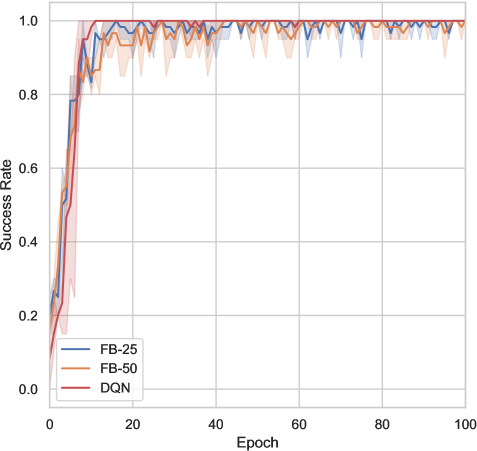
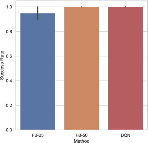
Figure 1: Comparative performance of FB for different dimensions and DQN in FetchReach. Left: success rate averaged over 20 randomly selected goals as function of the first 100 training epochs. Right: success rate averaged over 20 random goals after 800 training epochs.

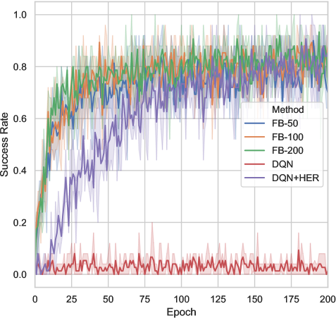
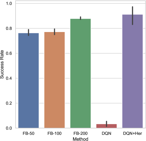
Figure 2: Comparative performance of FB for different dimensions and DQN in Ms. Pacman. Left: success rate averaged over 20 randomly selected goals as function of the first 200 training epochs. Right: success rate averaged over the goal space after 800 training epochs.

Figs. 1 and 2 show the comparative performance of FB for different dimensions $d$, and DQN respectively in FetchReach and Ms. Pacman (similar results in Discrete and Continuous Mazes are provided in Appendix D). In Ms. Pacman, DQN totally fails to learn and we had to add HER to make it work. The performance of FB consistently increases with the dimension $d$ and the best dimension matches the performance of the goal-oriented baseline.

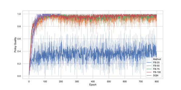
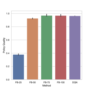
Figure 8: Discrete maze: Comparative performance of FB for different dimensions and DQN. Left: the policy quality averaged over 20 randomly selected goals as function of the training epochs. Right: the policy quality averaged over the goal space after 800 training epochs.

In Discrete Maze, we observe a drop of performance for $d=25$ (Appendix D, Fig. 8): this is due to the spatial smoothing induced by the small rank approximation and the reward being nonzero only if the agent is exactly at the goal. This spatial blurring is clear on heatmaps for $d=25$ vs $d=75$ (Fig. 3). With $d=25$ the agent often stops right next to its goal.

To evaluate the sample efficiency of FB, after each epoch, we evaluate the agent on 20 randomly selected goals. Learning curves are reported in Figs. 1 and 2 (left). In all environments, we observe no loss in sample efficiency compared to the goal-oriented baseline. In Ms. Pacman, FB even learns faster than DQN+HER.

5.3 More Complex Rewards: Qualitative Results

We now investigate FB’s ability to generalize to new tasks that cannot be solved by an already trained goal-oriented model: reaching a goal with forbidden states imposed a posteriori, reaching the nearest of two goals, and choosing between a small, close reward and a large, distant one.

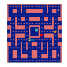
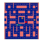
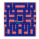
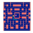
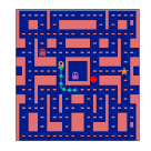
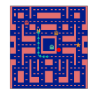
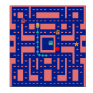
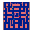
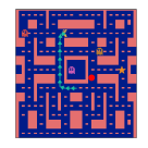
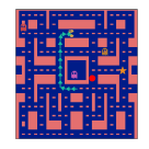
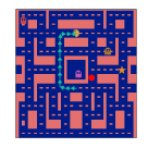
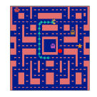
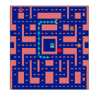
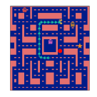
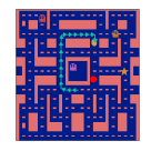
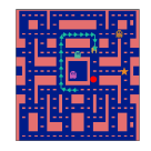
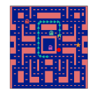
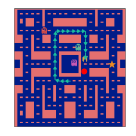
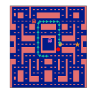
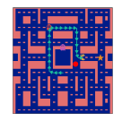
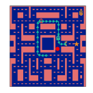
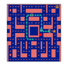
Figure 16: Full series of frames in Ms. Pacman along the trajectory generated by the $F^{\!\top}\!B$ policy for the task of reaching a target position (star shape ) while avoiding forbidden positions (red shape ).

First, for the task of reaching a target position $g_{0}$ while avoiding some forbidden positions $g_{1},\ldots g_{k}$ , we set $z_{R}=B(g_{1})-\lambda\sum_{i=1}^{k}B(g_{i})$ and run the corresponding $\varepsilon$-greedy policy defined by $F(s,a,z_{R})^{\top}z_{R}$. Fig. 5 shows the resulting trajectories, which succeed at solving the task for the different domains. In Ms. Pacman, the path is suboptimal (though successful) due to the sudden appearance of a monster along the optimal path. (We only plot the initial frame; see the full series of frames along the trajectory in Appendix D, Fig. 16.) Fig. 4 (left) provides a contour plot of $\max_{a\in A}F(s,a,z_{R})^{\top}z_{R}$ for the continuous maze and shows the landscape shape around the forbidden regions.

Next, we consider the task of reaching the closest target among two equally rewarding positions $g_{0}$ and $g_{1}$, by setting $z_{R}=B(g_{0})+B(g_{1})$. The optimal $Q$-function is not a linear combination of the $Q$-functions for $g_{0}$ and $g_{1}$. Fig. 6 shows successful trajectories generated by the policy $\pi_{z_{R}}$. On the contour plot of $\max_{a\in A}F(s,a,z_{R})^{\top}z_{R}$ in Fig. 4 (right), the two rewarding positions appear as basins of attraction. Similar results for a third task are shown in Appendix D: introducing a “distracting” small reward next to the initial position of the agent, with a larger reward further away.

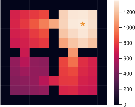
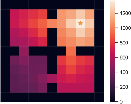
Figure 3: Heatmap of $\max_{a}F(s,a,z_{R})^{\top}z_{R}$ for $z_{R}=B(\text{ \leavevmode\hbox to8.27pt{\vbox to8.31pt{\text{[drawing]}}}})$ Left: $d=25$. Right: $d=75$.

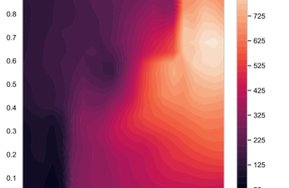
Figure 4: Contour plot of $\max_{a\in A}F(s,a,z_{R})^{\top}z_{R}$ in Continuous Maze. Left: for the task of reaching a target while avoiding a forbidden region, Right: for two equally rewarding targets.

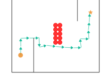
Figure 5: Trajectories generated by the $F^{\!\top}\!B$ policies for the task of reaching a target position (star shape while avoiding forbidden positions (red shape )

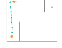
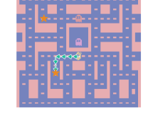
Figure 6: Trajectories generated by the $F^{\!\top}\!B$ policies for the task of reaching the closest among two equally rewarding positions (star shapes ). (Optimal $Q$-values are not linear over such mixtures.)

5.4 Embedding Visualizations

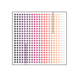
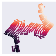
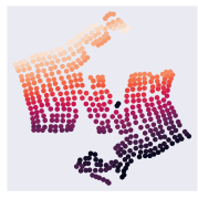
Figure 7: Visualization of FB embedding vectors on Continuous Maze after projecting them in two-dimensional space with t-SNE. Left: the states to be mapped. Middle: the $F$ embedding. Right: the $B$ embedding. The walls appear as large dents; the smaller dents correspond to the number of steps needed to get past a wall.

We visualize the learned FB state embeddings for Continuous Maze by projecting them into 2-dimensional space using t-SNE [VdMH08] in Fig. 7. For the forward embeddings, we set $z=0$ corresponding to the uniform policy. We can see that FB partitions states according to the topology induced by the dynamics: states on opposite sides of walls are separated in the representation space and states on the same side lie together. Appendix D includes embedding visualizations for different $z$ and for Discrete Maze and Ms. Pacman.

6 Related work

[BBQ⁺18] learn optimal policies for rewards that are linear combinations of a finite number of feature functions provided in advance by the user. This approach cannot tackle generic rewards or goal-oriented RL: this would require introducing one feature per possible goal state, requiring infinitely many features in continuous spaces.

Our approach does not require user-provided features describing the future tasks, thanks to using successor states [BTO21] where [BBQ⁺18] use successor features. Schematically, and omitting actions, successor features start with user-provided features $\varphi$, then learn $\psi$ such that $\psi(s_{0})=\sum_{t\geq 0}\gamma^{t}\operatorname{\mathbb{E}}[\varphi(s_{t})\mid s_{0}]$. This limits applicability to rewards that are linear combinations of $\varphi$. Here we use successor state probabilities, namely, we learn two representations $F$ and $B$ such that $F(s_{0})^{\!\top}\!B(s^{\prime})=\sum_{t\geq 0}\gamma^{t}\Pr\nolimits(s_{t}=s^{\prime}\mid s_{0})$. This does not require any user-provided input.

Thus we learn two representations instead of one. The learned backward representation $B$ is absent from [BBQ⁺18]. $B$ plays a different role than the user-provided features $\varphi$ of [BBQ⁺18]: if the reward is known a priori to depend only on some features $\varphi$, we learn $B$ on top of $\varphi$, which represents all rewards that depend linearly or nonlineary on $\varphi$. Up to a change of variables, [BBQ⁺18] is recovered by setting $B=\operatorname{Id}$ on top of $\varphi$, or $B=\varphi$ and $\varphi=\operatorname{Id}$, and then only training $F$.

We use a similar parameterization of policies by $F(s,a,z)^{\!\top}\!z$ as in [BBQ⁺18], for similar reasons, although $z$ encodes a different object.

Successor representations where first defined in [Day93] for finite spaces, corresponding to an older object from Markov chains, the fundamental matrix [KS60, Bré99, GS97]. [SBG17] argue for their relevance for cognitive science. For successor representations in continuous spaces, a finite number of features $\varphi$ are specified first; this can be used for generalization within a family of tasks, e.g., [BDM⁺17, ZSBB17, GHB⁺19, HDB⁺19]. [BTO21] moves from successor features to successor states by providing pointwise occupancy map estimates even in continuous spaces, without using the sparse reward $\mathbbm{1}_{s_{t}=s^{\prime}}$. We borrow a successor state learning algorithm from [BTO21]. [BTO21] also introduced simpler versions of $F$ and $B$ for a single, fixed policy; [BTO21] does not consider the every-optimal-policy setting.

There is a long literature on goal-oriented RL. For instance, [SHGS15] learn goal-dependent value functions, regularized via an explicit matrix factorization. Goal-dependent value functions have been investigated in earlier works such as [FD02] and [SMD⁺11]. Hindsight experience replay (HER) [ACR⁺17] improves the sample efficiency of multiple goal learning with sparse rewards. A family of rewards has to be specified beforehand, such as reaching arbitrary target states. Specifying rewards a posteriori is not possible: for instance, learning to reach target states does not extend to reaching the nearest among several goals, reaching a goal while avoiding forbidden states, or maximizing any dense reward.

Hierarchical methods such as options [SPS99] can be used for multi-task RL problems. However, policy learning on top of the options is still needed after the task is known.

For finite state spaces, [JKSY20] use reward-free interactions to build a training set that summarizes a finite environment, in the sense that any optimal policies later computed on this training set instead of the true environment are provably $\varepsilon$-optimal, for any reward. They prove tight bounds on the necessary set size. Policy learning still has to be done afterwards for each reward.

Acknowledgments.

The authors would like to thank Léonard Blier, Diana Borsa, Alessandro Lazaric, Rémi Munos, Tom Schaul, Corentin Tallec, Nicolas Usunier, and the anonymous reviewers for numerous comments, technical questions, references, and invaluable suggestions for presentation that led to an improved text.

7 Conclusion

The FB representation is a learnable mathematical object that “summarizes” a reward-free MDP. It provides near-optimal policies for any reward specified a posteriori, without planning. It is learned from black-box reward-free interactions with the environment. In practice, this unsupervised method performs comparably to goal-oriented methods for reaching arbitrary goals, but is also able to tackle more complex rewards in real time. The representations learned encode the MDP dynamics and may have broader interest.

Checklist

1. For all authors…

   1. Do the main claims made in the abstract and introduction accurately reflect the paper’s contributions and scope? [Yes]

   2. Did you describe the limitations of your work? [Yes] , Section 4

   3. Did you discuss any potential negative societal impacts of your work? [No] This is a theoretical work on fully generic methods for reinforcement learning. The potential impact is the same as that of reinforcement learning in general.

   4. Have you read the ethics review guidelines and ensured that your paper conforms to them? [Yes]

2. If you are including theoretical results…

   1. Did you state the full set of assumptions of all theoretical results? [Yes]

   2. Did you include complete proofs of all theoretical results? [Yes] , Appendix C.

3. If you ran experiments…

   1. Did you include the code, data, and instructions needed to reproduce the main experimental results (either in the supplemental material or as a URL)? [Yes] in the supplemental material.

   2. Did you specify all the training details (e.g., data splits, hyperparameters, how they were chosen)? [Yes] Appendix D

   3. Did you report error bars (e.g., with respect to the random seed after running experiments multiple times)? [Yes]

   4. Did you include the total amount of compute and the type of resources used (e.g., type of GPUs, internal cluster, or cloud provider)? [No]

4. If you are using existing assets (e.g., code, data, models) or curating/releasing new assets…

   1. If your work uses existing assets, did you cite the creators? [Yes] Appendix D.1

   2. Did you mention the license of the assets? [No]

   3. Did you include any new assets either in the supplemental material or as a URL? [No]

   4. Did you discuss whether and how consent was obtained from people whose data you’re using/curating? [N/A]

   5. Did you discuss whether the data you are using/curating contains personally identifiable information or offensive content? [N/A]

5. If you used crowdsourcing or conducted research with human subjects…

   1. Did you include the full text of instructions given to participants and screenshots, if applicable? [N/A]

   2. Did you describe any potential participant risks, with links to Institutional Review Board (IRB) approvals, if applicable? [N/A]

   3. Did you include the estimated hourly wage paid to participants and the total amount spent on participant compensation? [N/A]

Outline of the Supplementary Material

The Appendix is organized as follows.

• Appendix A presents the pseudo-code of the unsupervised phase of FB algorithm.

• Appendix B provides extended theoretical results on approximate solutions and general goals:

  • Section B.1 formalizes the forward-backward representation with a goal or feature space.

  • Section B.2 establishes the existence of exact FB representations in finite spaces, and discusses the influence of the dimension $d$.

  • Section B.3 shows how approximate solutions provide approximately optimal policies.

  • Section B.4 shows how $F$ and $B$ are successor and predecessor features of each other, and how the policies are optimal for rewards linearly spanned by $B$.

  • Section B.5 explains how to estimate $z_{R}$ at test time from a state distribution different from the training distribution.

  • Section B.6 presents a note of the measure $M^{\pi}$ and its density $m^{\pi}$.

• Appendix C provides proofs of all theoretical results above.

• Appendix D provides additional information about our experiments:

  • Section D.1 describes the environments.

  • Section D.2 describes the different architectures used for FB as well as the goal-oriented DQN.

  • Section D.3 provides implementation details and hyperparameters.

  • Section D.4 provides additional experimental results.

Appendix A Algorithm

The unsupervised phase of the FB algorithm is described in Algorithm 1.

The loss function for the Bellman equation on $F$ and $B$ appears on line 19, while the auxiliary loss function for orthonormalization of $B$ appears on line 21.

Algorithm 1 FB algorithm: Unsupervised Phase

1:  Inputs: replay buffer $\mathcal{D}$ , Polyak coefficient $\alpha$ , $\nu$ a probability distribution over $\mathbb{R}^{d}$, randomly initialized networks $F_{\theta}$ and $B_{\omega}$, learning rate $\eta$, mini-batch size $b$, number of episodes $E$, number of gradient updates $N$, temperature $\tau$ and regularization coefficient $\lambda$.

2:  for $m=1,\ldots$ do

3:     /* Collect $E$ episodes

4:     for episode $e=1,\ldots E$ do

5:        Sample $z\sim\nu$

6:        Observe an initial state $s_{0}$

7:        for $t=1,\ldots$ do

8:           Select an action $a_{t}$ according to some behaviour policy (e.g the $\varepsilon$-greedy with respect to $F_{\theta}(s_{t},a,z)^{\top}z$ )

9:           Observe next state $s_{t+1}$

10:           Store transition $(s_{t},a_{t},s_{t+1})$ in the replay buffer $\mathcal{D}$

11:        end for

12:     end for

13:     /* Perform $N$ stochastic gradient descent updates

14:     for  $n=1\ldots N$ do

15:        Sample a mini-batch of transitions $\{(s_{i},a_{i},s_{i+1})\}_{i\in I}\subset\mathcal{D}$ of size $|I|=b$.

16:        Sample a mini-batch of target state-action pairs $\{(s^{\prime}_{i},a^{\prime}_{i})\}_{i\in I}\subset\mathcal{D}$ of size $|I|=b$.

17:        Sample a mini-batch of $\{z_{i}\}_{i\in I}\sim\nu$ of size $|I|=b$.

18:        Set $\pi_{z_{i}}(\cdot\mid s_{i+1})=\texttt{softmax}(F_{\theta^{-}}(s_{i+1},\cdot,z_{i})^{\top}z_{i}/\tau)$

19:        $\mathscr{L}(\theta,\omega)=$$\frac{1}{2b^{2}}\sum_{i,j\in I^{2}}\left(F_{\theta}(s_{i},a_{i},z_{i})^{\top}B_{\omega}(s^{\prime}_{j},a^{\prime}_{j})-\gamma\sum_{a\in A}\pi_{z_{i}}(a\mid s_{i+1})\cdot F_{\theta^{-}}(s_{i+1},a,z_{i})^{\top}B_{\omega^{-}}(s^{\prime}_{j},a^{\prime}_{j})\right)^{2}-\frac{1}{b}\sum_{i\in I}F_{\theta}(s_{i},a_{i},z_{i})^{\top}B_{\omega}(s_{i},a_{i})$

20:        /* Compute orthonormality regularization loss

21:        $\mathscr{L}_{\texttt{reg}}(\omega)=\frac{1}{b^{2}}\sum_{i,j\in I^{2}}B_{\omega}(s_{i},a_{i})^{\top}\texttt{stop-gradient}(B_{\omega}(s^{\prime}_{j},a^{\prime}_{j}))\cdot\texttt{stop-gradient}(B_{\omega}(s_{i},a_{i})^{\top}B_{\omega}(s^{\prime}_{j},a^{\prime}_{j}))-\frac{1}{b}\sum_{i\in I}B_{\omega}(s_{i},a_{i})^{\top}\texttt{stop-gradient}(B_{\omega}(s_{i},a_{i}))$

22:        Update $\theta\leftarrow\theta-\eta\nabla_{\theta}\mathscr{L}(\theta,\omega)$ and $\omega\leftarrow\omega-\eta\nabla_{\omega}(\mathscr{L}(\theta,\omega)+\lambda\cdot\mathscr{L}_{\texttt{reg}}(\omega))$

23:     end for

24:     /* Update target network parameters

25:     $\theta^{-}\leftarrow\alpha\theta^{-}+(1-\alpha)\theta$

26:     $\omega^{-}\leftarrow\alpha\omega^{-}+(1-\alpha)\omega$

27:  end for

Appendix B Extended Results: Approximate Solutions and General Goals

Notation.

In general, we denote by $M^{\pi}$ the successor measure of policy $\pi$ as defined in (1), and by $m^{\pi}$ its density, if it exists, with respect to a reference measure $\rho$. Namely,

$$M^{\pi}(s_{0},a_{0},\operatorname{d}\!{}s,\operatorname{d}\!{}a)=m^{\pi}(s_{0},a_{0},s,a)\rho(\operatorname{d}\!{}s,\operatorname{d}\!{}a).$$ (9)

Thus, the defining property of forward-backward representations (Definition 1) is $F(s_{0},a_{0},z)^{\!\top}\!B(s,a)=m^{\pi_{z}}(s_{0},a_{0},s,a)$.

We use the same convention for parametric models, with $M^{\pi}_{\theta}$ a measure and $m^{\pi}_{\theta}$ its density. The reference measure $\rho$ is fixed and may be unknown (typically $\rho$ is the distribution of state-actions in a training set or under an exploration policy).

B.1 The Forward-Backward Representation With a Goal or Feature Space

Here we state a generalization of Theorem 2 covering some extensions mentioned in the text.

First, this covers rewards known to only depend on certain features $g=\varphi(s,a)$ of the state-action $(s,a)$, where $\varphi$ is a known function with values in some goal state $G$ (for instance, rewards depending only on some components of the state). Then it is enough to compute $B$ as a function of the goal $g$. Theorem 2 corresponds to $\varphi=\operatorname{Id}$. This is useful to introduce prior information when available, resulting in a smaller model $(F,B)$.

This also recovers successor features as in [BBQ⁺18], defined by user-provided features $\varphi$. Indeed, fixing $B$ to $\operatorname{Id}$ and setting our $\varphi$ to the $\varphi$ of [BBQ⁺18] (or fixing $B$ to their $\varphi$ and our $\varphi$ to $\operatorname{Id}$) will represent the same set of rewards and policies as in [BBQ⁺18], namely, optimal policies for rewards linear in $\varphi$ (although with a slightly different learning algorithm and up to a linear change of variables for $F$ and $z$ given by the covariance of $\varphi$, see Appendix B.4). More generally, keeping the same $\varphi$ but letting $B$ free (with larger $d$) can provide optimal policies for rewards that are arbitrary functions of $\varphi$, linear or not.

For this, we extend successor state measures to values in goal spaces, representing the discounted time spent at each goal by the policy. Namely, given a policy $\pi$, let $M^{\pi}$ be the the successor state measure of $\pi$ over goals $g$:

$$M^{\pi}(s,a,\operatorname{d}\!{}g)\mathrel{\mathop{:}}=\sum_{t\geq 0}\gamma^{t}\Pr\nolimits\left(\varphi(s_{t},a_{t})\in\operatorname{d}\!{}g\mid s_{0}=s,\,a_{0}=a,\,\pi\right)$$ (10)

for each state-action $(s,a)$ and each measurable set $\operatorname{d}\!{}g\subset G$. This will be the object approximated by $F(s,a,z)^{\!\top}\!B(g)$.

Second, we use a more general model of successor states: instead of $m\approx F^{\!\top}\!B$ we use $m\approx F^{\!\top}\!B+\bar{m}$ where $\bar{m}$ does not depend on the action, so that the $F^{\!\top}\!B$ part only computes advantages. This lifts the constraint that the model of $m$ has rank at most $d$, because there is no restriction on the rank on $\bar{m}$: the rank restriction only applies to the advantage function.

Third, we state a form of policy improvement for the FB representation. Namely, the $Q$-function $F(s,a,z_{R})^{\!\top}\!z_{R}$ for a given reward can be computed as a supremum over all values of $z$.

For simplicity we state the result with deterministic rewards, but this extends to stochastic rewards, because the expectation $z_{R}$ will be the same.

Definition 3 (Extended forward-backward representation of an MDP).

Consider an MDP with state space $S$ and action space $A$. Let $\varphi\colon S\times A\to G$ be a function from state-actions to some goal space $G={\mathbb{R}}^{k}$.

Let $Z={\mathbb{R}}^{d}$ be some representation space. Let

$$F\colon S\times A\times Z\to Z,\qquad B\colon G\to Z,\qquad\bar{m}\colon S\times Z\times G\to{\mathbb{R}}$$ (11)

be three functions. For each $z\in Z$, define the policy

$$\pi_{z}(a|s)\mathrel{\mathop{:}}=\operatorname*{arg\,max}_{a}F(s,a,z)^{\!\top}\!z.$$ (12)

Let $\rho$ be any measure over the goal space $G$.

We say that $F$, $B$, and $\bar{m}$ are an extended forward-backward representation of the MDP with respect to $\rho$, if the following holds: for any $z\in Z$, any state-actions $(s,a)$, and any goal $g\in G$, one has

$$M^{\pi_{z}}(s,a,\operatorname{d}\!{}g)=\left(F(s,a,z)^{\!\top}\!B(g)+\bar{m}(s,z,g)\right)\rho(\operatorname{d}\!{}g)$$ (13)

where $M^{\pi_{z}}$ is the successor state measure (10) of policy $\pi_{z}$.

Theorem 4 (Forward-backward representation of an MDP, with features as goals).

Consider an MDP with state space $S$ and action space $A$. Let $\varphi\colon S\times A\to G$ be a function from state-actions to some goal space $G={\mathbb{R}}^{k}$.

Let $F$, $B$, and $\bar{m}$ be an extended forward-backward representation of the MDP with respect to some measure $\rho$ over $G$.

Then the following holds. Let $R\colon S\times A\to{\mathbb{R}}$ be any bounded reward function, and assume that this reward function depends only on $g=\varphi(s,a)$, namely, that there exists a function $r\colon G\to{\mathbb{R}}$ such that $R(s,a)=r(\varphi(s,a))$. Set

$$z_{R}\mathrel{\mathop{:}}=\int_{g\in G}r(g)B(g)\,\rho(\operatorname{d}\!{}g)$$ (14)

assuming the integral exists.

Then:

1. $\pi_{z_{R}}$ is an optimal policy for reward $R$ in the MDP.

2. For any $z\in Z$, the $Q$-function of policy $\pi_{z}$ for the reward $R$ is equal to

   $$Q^{\pi_{z}}(s,a)=F(s,a,z)^{\!\top}\!z_{R}+\bar{V}^{z}(s)$$ (15)

   and the optimal $Q$-function $Q^{\star}_{R}$ is obtained when $z=z_{R}$:

   $$Q^{\star}_{R}(s,a)=F(s,a,z_{R})^{\!\top}\!z_{R}+\bar{V}^{z_{R}}(s).$$ (16)

   Here

   $$\bar{V}^{z}(s)\mathrel{\mathop{:}}=\int_{g\in G}\bar{m}(s,z,g)r(g)\,\rho(\operatorname{d}\!{}g)$$ (17)

   and in particular $\bar{V}=0$ if $\bar{m}=0$.

   The advantages $Q^{\pi_{z}}(s,a)-Q^{\pi_{z}}(s,a^{\prime})$ do not depend on $\bar{V}$, so computing $\bar{V}$ is not necessary to obtain the policies.

3. If $\bar{m}=0$, then for any state-action $(s,a)$ one has

   $$Q^{\star}_{R}(s,a)=F(s,a,z_{R})^{\!\top}\!z_{R}=\sup_{z\in Z}F(s,a,z)^{\!\top}\!z_{R}.$$ (18)

(We do not claim that $\bar{V}$ is the value function and $F^{\!\top}\!z_{R}$ the advantage function, only that the sum is the $Q$-function. When $\bar{m}=0$, the term $F^{\!\top}\!z_{R}$ is the whole $Q$-function.)

The last point of the theorem is a form of policy improvement. Indeed, by the second point, $F(s,a,z)^{\!\top}\!z_{R}$ is the estimated $Q$-function of policy $\pi_{z}$ for rewards $r$. This may be useful if $z_{R}$ falls outside of the training distribution for $F$: then the values of $F(s,a,z_{R})$ may not be safe to use. In that case, it may be useful to use a finite set $Z^{\prime}\subset Z$ of values of $z$ closer to the training distribution, and use the estimate $\sup_{z\in Z^{\prime}}F(s,a,z)^{\!\top}\!z_{R}$ instead of $F(s,a,z_{R})^{\!\top}\!z_{R}$ for the optimal $Q$-function. A similar option has been used, e.g., in [BBQ⁺18], but in the end it was not necessary in our experiments.

Remark 5.

Formally, the statement holds for arbitrary $\rho$, but it only makes sense if $\rho$ has full support (or at least covers all reachable parts of the state space): (13) requires the support of $M^{\pi_{z}}$ to be included in that of $\rho$. Otherwise, FB representations may not exist and the statement is empty.

B.2 Existence of Exact $FB$ Solutions, Influence of Dimension $d$, Uniqueness

Existence of exact $FB$ representations in finite spaces.

We now prove existence of an exact solution for finite spaces if the representation dimension $d$ is at least $\#S\times\#A$. Solutions are never unique: one may always multiply $F$ by an invertible matrix $C$ and multiply $B$ by $(C^{\!\top}\!)^{-1}$, see Remark 7 below (this allows us to impose orthonormality of $B$ in the experiments).

The constraint $d\geq\#S\times\#A$ can be largely overestimated depending on the tasks of interest, though. For instance, we prove below that in an $n$-dimensional toric grid $S=\{1,\ldots,k\}^{n}$, $d=2n$ is enough to obtain optimal policies for reaching every target state (a set of tasks smaller than optimizing all possible rewards).

Proposition 6 (Existence of an exact $FB$ representation for finite state spaces).

Assume that the state and action spaces $S$ and $A$ of an MDP are finite. Let $Z={\mathbb{R}}^{d}$ with $d\geq\#S\times\#A$. Let $\rho$ be any measure on $S\times A$, with $\rho(s,a)>0$ for any $(s,a)$.

Then there exists $F\colon S\times A\times Z\to Z$ and $B\colon S\times A\to Z$, such that $F^{\!\top}\!B$ is equal to the successor state density of $\pi_{z}$ with respect to $\rho$:

$$F^{\!\top}\!(s,a,z)B(s^{\prime},a^{\prime})=\sum_{t\geq 0}\gamma^{t}\frac{\Pr\nolimits((s_{t},a_{t})=(s^{\prime},a^{\prime})\mid s_{0}=s,\,a_{0}=a,\,\pi_{z})}{\rho(s^{\prime},a^{\prime})}$$ (19)

for any $z\in Z$ and any state-actions $(s,a)$ and $(s^{\prime},a^{\prime})$, where $\pi_{z}$ is defined as in Definition 1 by $\pi_{z}(s)=\operatorname*{arg\,max}_{a}F(s,a,z)^{\!\top}\!z$.

A small dimension $d$ can be enough for navigation: examples.

In practice, even a small $d$ can be enough to get optimal policies for reaching arbitrary many states (as opposed to optimizing all possible rewards). Let us give an example with $S$ a toric $n$-dimensional grid of size $k$.

Let us start with $n=1$. Take $S=\{0,\ldots,k-1\}$ to be a length-$k$ cycle with three actions $a\in\{-1,0,1\}$ (go left, stay in place, go right). Take $d=2$, so that $Z={\mathbb{R}}^{2}\simeq{\mathbb{C}}$.

We consider the tasks of reaching an arbitrary target state $s^{\prime}$, for every $s^{\prime}\in S$. Thus the goal state is $G=S$ in the notation of Theorem 4, and $B$ only depends on $s^{\prime}$. The policy for such a reward is $\pi_{z_{R}}=\pi_{B(s^{\prime})}$.

For a state $s\in\{0,\ldots,k-1\}$ and action $a\in\{-1,0,1\}$, define

$$F(s,a,z)\mathrel{\mathop{:}}=e^{2i\pi(s+a)/k},\qquad B(s)\mathrel{\mathop{:}}=e^{2i\pi s/k}.$$ (20)

Then one checks that $\pi_{B(s^{\prime})}$ is the optimal policy for reaching $s^{\prime}$, for every $s^{\prime}\in S$. Indeed, $F(s,a,z_{R})^{\!\top}\!z_{R}=\cos(2\pi(s+a-s^{\prime})/k)$. This is maximized for the action $a$ that brings $s$ closer to $s^{\prime}$.

So the policies will be optimal for reaching every target $s^{\prime}\in S$, despite the dimension being only $2$.

By taking the product of $n$ copies of this example, this also works on the $n$-dimensional toric grid $S=\{0,\ldots,k-1\}^{n}$ with $2n+1$ actions (add $\pm 1$ in each direction or stay in place), with a representation of dimension $d=2n$ in ${\mathbb{C}}^{n}$, namely, by taking $B(s)_{j}\mathrel{\mathop{:}}=e^{2i\pi s_{j}/k}$ for ecah direction $j$ and likewise for $F$. Then $\pi_{B(s^{\prime})}$ is the optimal policy for reaching $s^{\prime}$ for every $s^{\prime}\in S$.

More generally, if one is only interested in the optimal policies for reaching states, then it is easy to show that there exist functions $F\colon S\times A\to Z$ and $B\colon S\to Z$ such that the policies $\pi_{z}$ describe the optimal policies to reach each state: it is enough that $B$ be injective (typically requiring $d=\dim(S)$). Indeed, for any state $s\in S$, let $\pi^{\star}_{s}$ be the optimal policy to reach $s$. We want $\pi_{z}$ to be equal to $\pi^{\star}_{s}$ for $z=B(s)$ (the value of $z_{R}$ for a reward located at $s$). This translates as $\operatorname*{arg\,max}_{a}F(s^{\prime},a,B(s))^{\!\top}\!B(s)=\pi^{\star}_{s}(s^{\prime})$ for every other state $s^{\prime}$. This is realized just by letting $F$ be any function such that $F(s^{\prime},\pi^{\star}_{s}(s^{\prime}),B(s))\mathrel{\mathop{:}}=B(s)$ and $F(s^{\prime},a,B(s))\mathrel{\mathop{:}}=-B(s)$ for every other action $a$. As soon as $B$ is injective, there exists such a function $F$. (Unfortunately, we are not able to show that the learning algorithm reaches such a solution.)

Let us turn to uniqueness of $F$ and $B$.

Remark 7.

Let $C$ be an invertible $d\times d$ matrix. Given $F$ and $B$ as in Theorem 2, define

$$B^{\prime}(s,a)\mathrel{\mathop{:}}=CB(s,a),\qquad F^{\prime}(s,a,z)\mathrel{\mathop{:}}=(C^{\!\top}\!)^{-1}F(s,a,C^{-1}z)$$ (21)

together with the policies $\pi^{\prime}_{z}(s)\mathrel{\mathop{:}}=\operatorname*{arg\,max}_{a}F^{\prime}(s,a,z)^{\!\top}\!z$. For each reward $r$, define $z^{\prime}_{R}\mathrel{\mathop{:}}=\operatorname{\mathbb{E}}_{(s,a)\sim\rho}[r(s,a)B^{\prime}(s,a)]$.

Then this operation does not change the policies or estimated $Q$-values: for any reward, we have $\pi^{\prime}_{z^{\prime}_{R}}=\pi_{z_{R}}$, and $F^{\prime}(s,a,z^{\prime}_{R})^{\!\top}\!z^{\prime}_{R}=F(s,a,z_{R})^{\!\top}\!z_{R}$.

In particular, assume that the components of $B$ are linearly independent. Then, taking $C=\left(\operatorname{\mathbb{E}}_{(s,a)\sim\rho}B(s,a)B(s,a)^{\!\top}\!\right)^{-1/2}$, $B^{\prime}$ is $L^{2}(\rho)$-orthonormal. So up to reducing the dimension $d$ to $\operatorname{rank}(B)$, we can always assume that $B$ is $L^{2}(\rho)$-orthonormal, namely, that $\operatorname{\mathbb{E}}_{(s,a)\sim\rho}B(s,a)B(s,a)^{\!\top}\!=\operatorname{Id}$.

Reduction to orthonormal $B$ will be useful in some proofs below. Even after imposing that $B$ be orthonormal, solutions are not unique, as one can still apply a rotation matrix on the variable $z$.

For a single policy $\pi_{z}$, the $F^{\!\top}\!B$ decomposition may be further standardized in several ways: after a linear change of variables in ${\mathbb{R}}^{d}$, and up to decreasing $d$ by removing unused directions in ${\mathbb{R}}^{d}$, one may assume either that $\operatorname{Cov}_{\rho}B=\operatorname{Id}$ and $\operatorname{Cov}_{\rho}F$ is diagonal, or that $\operatorname{Cov}_{\rho}F=\operatorname{Cov}_{\rho}B$ is diagonal, or write the decomposition as $\tilde{F}^{\!\top}\!D\tilde{B}$ with $D$ diagonal and $\operatorname{Cov}_{\rho}\tilde{F}=\operatorname{Cov}_{\rho}\tilde{B}=\operatorname{Id}$, thus corresponding to an approximation of the singular value decomposition of the successor measure $M^{\pi_{z}}$ in $L^{2}(\rho)$. However, since $B$ is shared between all values of $z$ and all policies $\pi_{z}$, it is a priori not possible to realize this for all $z$ simultaneously.

B.3 Approximate Solutions Provide Approximately Optimal Policies

Here we prove that the optimality in Theorems 2 and 4 is robust to approximation errors during training: approximate solutions still provide approximately optimal policies. We deal first with the approximation errors on $(F,B)$ during unsupervised training, then on $z_{R}$ during the reward estimation phase (in case the reward is not known explicity).

B.3.1 Influence of Approximate $F$ and $B$: Optimality Gaps are Proportional to $m^{\pi}-F^{\!\top}\!B$

In continuous spaces, Theorems 2 and 4 are somewhat spurious: the equality $F^{\!\top}\!B=m$ that defines FB representations will never hold exactly with finite representation dimension $d$. Instead, $F^{\!\top}\!B$ will only be a rank-$d$ approximation of $m$. Even in finite spaces, since $F$ and $B$ are learned by a neural network, we can only expect that $F^{\!\top}\!B\approx m$ in general. Therefore, we provide results that extend Theorems 2 and 4 to approximate training and approximate FB representations.

Optimality gaps are directly controlled by the error $m^{\pi}-F^{\!\top}\!B$ on the solution $F^{\!\top}\!B$. We provide this result for different notions of approximations between $m^{\pi}$ and $F^{\!\top}\!B$. First, in sup norm over $(s,a)$ but in expectation over $(s^{\prime},a^{\prime})$ (so that a perfect model of the successor states $(s^{\prime},a^{\prime})$ of each $(s,a)$ is not necessary, only an average model). Second, for the weak topology on measures (this is the most relevant in continuous spaces: for instance, a Dirac measure can be approached by a continuous model in the weak topology). Finally, we provide pointwise estimates instead of only norms: for any reward, we show that the optimality gaps at each state can be bounded by an explicit matrix product directly involving the FB error matrix $m^{\pi}-F^{\!\top}\!B$ (Theorem 9).

$F$ and $B$ are trained such that $F(s,a,z)^{\!\top}\!B(s^{\prime},a^{\prime})$ approximates the successor state density $m^{\pi_{z}}(s,a,s^{\prime},a^{\prime})$. In the simplest case, we prove that if for some reward $R$,

$$\operatorname{\mathbb{E}}_{(s^{\prime},a^{\prime})\sim\rho}\left\lvert F(s,a,z_{R})^{\!\top}\!B(s^{\prime},a^{\prime})-m^{\pi_{z_{R}}}(s,a,s^{\prime},a^{\prime})\right\rvert\leq\varepsilon$$ (22)

for every $(s,a)$, then the optimality gap of policy $\pi_{z_{R}}$ is at most $(3\varepsilon/(1-\gamma))\sup\left\lvert R\right\rvert$ for that reward (Theorem 8, first case).

In continuous spaces, $m^{\pi}$ is usually a distribution (Appendix B.6), so such an approximation will not hold, and it is better to work on the measures themselves rather than their densities, namely, to compare $F^{\!\top}\!B\rho$ to $M^{\pi}$ instead of $F^{\!\top}\!B$ to $m^{\pi}$. We prove that if $F^{\!\top}\!B\rho$ is close to $M^{\pi}$ in the weak topology, then the resulting policies are optimal for any Lipschitz reward.

Remember that a sequence of nonnegative measures $\mu_{n}$ converges weakly to $\mu$ if for any bounded, continuous function $f$, $\int f(x)\mu_{n}(dx)$ converges to $\int f(x)\mu(\operatorname{d}\!{}x)$ ([Bog07], §8.1). The associated topology can be defined via the following Kantorovich–Rubinstein norm on nonnegative measures ([Bog07], §8.3)

$$\left\lVert\mu-\mu^{\prime}\right\rVert_{\mathrm{KR}}\mathrel{\mathop{:}}=\sup\left\{\left\lvert\int f(x)\mu(\operatorname{d}\!{}x)-\int f(x)\mu^{\prime}(\operatorname{d}\!{}x)\right\rvert:\,f\text{ $1$-Lipschitz function with }\sup\left\lvert f\right\rvert\leq 1\right\}$$ (23)

where we have equipped the state-action space with any metric compatible with its topology.

The following theorem states that if $F^{\!\top}\!B$ approximates the successor state density of the policy $\pi_{z}$ (for various sorts of approximations), then $\pi_{z}$ is approximately optimal. Given a reward function $r$ on state-actions, we denote

$$\left\lVert r\right\rVert_{\infty}\mathrel{\mathop{:}}=\sup_{(s,a)\in S\times A}\left\lvert r(s,a)\right\rvert$$ (24)

and

$$\left\lVert r\right\rVert_{\mathrm{Lip}}\mathrel{\mathop{:}}=\sup_{(s,a)\neq(s^{\prime},a^{\prime})\in S\times A}\frac{r(s,a)-r(s^{\prime},a^{\prime})}{d((s,a),(s^{\prime},a^{\prime}))}$$ (25)

where we have chosen any metric on state-actions.

The first statement is for any bounded reward. The second statement only assumes an $F^{\!\top}\!B$ approximation in the weak topology but only applies to Lipschitz rewards. The third statement is more general and is how we prove the first two: weaker assumptions on $F^{\!\top}\!B$ work on a stricter class of rewards.

Theorem 8 (If $F$ and $B$ approximate successor states, then the policies $\pi_{z}$ yield approximately optimal returns).

Let $F\colon S\times A\times Z\to Z$ and $B\colon S\times A\to Z$ be any functions, and define the policy $\pi_{z}(s)=\operatorname*{arg\,max}_{a}F(s,a,z)^{\!\top}\!z$ for each $z\in Z$.

Let $\rho$ be any positive probability distribution on $S\times A$, and for each policy $\pi$, let $m^{\pi}$ be the density of the successor state measure $M^{\pi}$ of $\pi$ with respect to $\rho$. Let

$$\hat{m}^{z}(s,a,s^{\prime},a^{\prime})\mathrel{\mathop{:}}=F(s,a,z)^{\!\top}\!B(s^{\prime},a^{\prime}),\qquad\hat{M}^{z}(s,a,\operatorname{d}\!{}s^{\prime},\operatorname{d}\!{}a^{\prime})\mathrel{\mathop{:}}=\hat{m}^{z}(s,a,s^{\prime},a^{\prime})\rho(\operatorname{d}\!{}s^{\prime},\operatorname{d}\!{}a^{\prime})$$ (26)

be the estimates of $m$ and $M$ obtained via the model $F$ and $B$.

Let $r\colon S\times A\to{\mathbb{R}}$ be any bounded reward function. Let $V^{\star}$ be the optimal value function for this reward $r$. Let $\hat{V}^{\pi_{z}}$ be the value function of policy $\pi_{z}$ for this reward. Let $z_{R}=\operatorname{\mathbb{E}}_{(s,a)\sim\rho}[r(s,a)B(s,a)]$.

Then:

1. If $\operatorname{\mathbb{E}}_{(s^{\prime},a^{\prime})\sim\rho}\left\lvert\hat{m}^{z_{R}}(s,a,s^{\prime},a^{\prime})-m^{\pi_{z_{R}}}(s,a,s^{\prime},a^{\prime})\right\rvert\leq\varepsilon$ for any $(s,a)$ in $S\times A$, then $\left\lVert\hat{V}^{\pi_{z_{R}}}-V^{\star}\right\rVert_{\infty}\leq 3\varepsilon\left\lVert r\right\rVert_{\infty}/(1-\gamma)$.

2. If $r$ is Lipschitz and $\left\lVert\hat{M}^{z_{R}}(s,a,\cdot)-M^{\pi_{z_{R}}}(s,a,\cdot)\right\rVert_{\mathrm{KR}}\leq\varepsilon$ for any $(s,a)\in S\times A$, then $\left\lVert\hat{V}^{\pi_{z_{R}}}-V^{\star}\right\rVert_{\infty}\leq 3\varepsilon\max(\left\lVert r\right\rVert_{\infty},\left\lVert r\right\rVert_{\mathrm{Lip}})/(1-\gamma)$.

3. More generally, let $\left\lVert\cdot\right\rVert_{A}$ be a norm on functions and $\left\lVert\cdot\right\rVert_{B}$ a norm on measures, such that $\int f\operatorname{d}\!{}\mu\leq\left\lVert f\right\rVert_{A}\left\lVert\mu\right\rVert_{B}$ for any function $f$ and measure $\mu$. Then for any reward function $r$ such that $\left\lVert r\right\rVert_{A}<\infty$,

   $$\left\lVert\hat{V}^{\pi_{z_{R}}}-V^{\star}\right\rVert_{\infty}\leq\frac{3\left\lVert r\right\rVert_{A}}{1-\gamma}\sup_{s,a}\left\lVert\hat{M}^{z_{R}}(s,a,\cdot)-M^{\pi_{z_{R}}}(s,a,\cdot)\right\rVert_{B}.$$ (27)

   Moreover, the optimal $Q$-function is close to $F(s,a,z_{R})^{\!\top}\!z_{R}$:

   $$\sup_{s,a}\left\lvert F(s,a,z_{R})^{\!\top}\!z_{R}-Q^{\star}(s,a)\right\rvert\leq\frac{2\left\lVert r\right\rVert_{A}}{1-\gamma}\sup_{s,a}\left\lVert\hat{M}^{z_{R}}(s,a,\cdot)-M^{\pi_{z_{R}}}(s,a,\cdot)\right\rVert_{B}.$$ (28)

Pointwise optimality gaps.

We now turn to a more precise estimation of the optimality gap at each state, expressed directly as a matrix product involving the FB error $m^{\pi}-F^{\!\top}\!B$.

Here we assume that the state space is finite: this is not essential but simplifies notation since everything can be represented as matrices and vectors. For each stochastic policy $\pi\colon S\to\mathrm{Prob}(A)$, we denote $P_{\pi}$ the associated stochastic matrix on state-actions:

$$(P_{\pi})_{(sa)(s^{\prime}a^{\prime})}\mathrel{\mathop{:}}=P(s^{\prime}|s,a)\pi(s^{\prime})[a^{\prime}].$$ (29)

We also view rewards and $Q$-functions as vectors indexed by state-actions.

Theorem 9.

Assume that the state space is finite. Let $F\colon S\times A\times{\mathbb{R}}^{d}\to{\mathbb{R}}^{d}$ and $B\colon S\times A\to{\mathbb{R}}^{d}$ be any functions. Define $\pi_{z}$ as in Definition 1. Let $\rho>0$ be any probability distribution over state-actions, and let $m^{\pi}$ be the successor density (9) of policy $\pi$ with respect to $\rho$.

For each $z\in{\mathbb{R}}^{d}$, define the FB error $E(z)$ as a matrix over state-actions:

$$E(z)_{(sa)(s^{\prime}a^{\prime})}\mathrel{\mathop{:}}=m^{\pi_{z}}(s,a,s^{\prime},a^{\prime})-F(s,a,z)^{\!\top}\!B(s^{\prime},a^{\prime}).$$ (30)

Let $r$ be any reward function and let $Q^{\star}$ and $\pi^{\star}$ be its optimal $Q$-function and policy. Let $z_{R}=\operatorname{\mathbb{E}}_{\rho}[r.B]$ as in Theorem 2, and let $Q^{\pi_{z_{R}}}$ be the $Q$-function of policy $\pi_{z_{R}}$.

Then we have the componentwise inequality between state-action vectors

$$0\leq Q^{\star}-Q^{\pi_{z_{R}}}\leq\left(\sum_{t\geq 0}\gamma^{t+1}P_{\pi^{\star}}^{t}\right)\left(P_{\pi^{\star}}-P_{\pi_{z_{R}}}\right)E(z_{R})\operatorname{diag}(\rho)\,r.$$ (31)

In particular, if $E(z_{R})=0$ then $\pi_{z_{R}}$ is optimal for reward $r$.

The matrix $\sum_{t\geq 0}\gamma^{t+1}P_{\pi^{\star}}^{t}$ represents states visited along the optimal trajectory starting at the initial state. Multiplying by $(P_{\pi^{\star}}-P_{\pi_{z_{R}}})$ visits states one step away from this trajectory. Therefore, what matters are the values of the FB error matrix $E(z_{R})_{(sa)(s^{\prime}a^{\prime})}$ at state-actions $(s,a)$ one step away from the optimal trajectories.

In unsupervised RL, we have no control over the first part $\sum_{t\geq 0}\gamma^{t+1}P_{\pi^{\star}}^{t}$, which depends only on the optimal trajectories of the unknown future tasks $r$. Therefore, in general it makes sense to just minimize $E(z)$ in some matrix norm, for as many values of $z$ as possible. (The choice of matrix norm influences which rewards will be best optimized, as illustrated by Theorem 8.)

B.3.2 An approximate $z_{R}$ yields an approximately optimal policy

We now turn to the second source of approximation: computing $z_{R}$ in the reward estimation phase. This is a problem only if the reward is not specified explicitly.

We deal in turn with the effect of using a model of the reward function, and the effect of estimating $z_{R}=\operatorname{\mathbb{E}}_{(s,a)\sim\rho}r(s,a)B(s,a)$ via sampling.

Which of these options is better depends a lot on the situation. If training of $F$ and $B$ is perfect, by construction the policies are optimal for each $z_{R}$: thus, estimating $z_{R}$ from rewards sampled at $N$ states $(s_{i},a_{i})\sim\rho$ will produce the optimal policy for exactly that empirical reward, namely, a nonzero reward at each $(s_{i},a_{i})$ but zero everywhere else, thus overfitting the reward function. Reducing the dimension $d$ reduces this effect, since rewards are projected on the span of the features in $B$: $B$ plays both the roles of a transition model and a reward regularizer. This appears as a $\sqrt{d/N}$ factor in Theorem 12 below.

Thus, if both the number of samples to train $F$ and $B$ and the number of reward samples are small, using a smaller $d$ will regularize both the model of the environment and the model of the reward. However, if the number of samples to train $F$ and $B$ is large, yielding an excellent model of the environment, but the number of reward samples is small, then learning a model of the reward function will be a better option than direct empirical estimation of $z_{R}$.

The first result below states that reward misidentification comes on top of the approximation error of the $F^{\!\top}\!B$ model. This is relevant, for instance, if a reward model $\hat{r}$ is estimated by an external model using some reward values.

Proposition 10 (Influence of estimating $z_{R}$ by an approximate reward).

Assume $\rho$ is a probability distribution. Let $\hat{r}\colon S\times A\to{\mathbb{R}}$ be any reward function. Let $\hat{z}_{R}=\operatorname{\mathbb{E}}_{(s,a)\sim\rho}[\hat{r}(s,a)B(s,a)]$.

Let $\varepsilon_{FB}$ be the error attained by the $F^{\!\top}\!B$ model in Theorem 8 for reward $\hat{r}$; namely, assume that $\left\lVert\hat{V}^{\pi_{\hat{z}_{R}}}-\hat{V}^{\star}\right\rVert_{\infty}\leq\varepsilon_{FB}$ with $\hat{V}^{\star}$ the optimal value function for $\hat{r}$.

Then the policy $\pi_{\hat{z}_{R}}(s)=\operatorname*{arg\,max}_{a}F(s,a,\hat{z}_{R})^{\!\top}\!\hat{z}_{R}$ defined by the model $\hat{r}$ is $\displaystyle\left(\frac{2\left\lVert r-\hat{r}\right\rVert_{\infty}}{(1-\gamma)}+\varepsilon_{FB}\right)$-optimal for reward $r$.

This still assumes that the expectation $\hat{z}_{R}=\operatorname{\mathbb{E}}_{(s,a)\sim\rho}[\hat{r}(s,a)B(s,a)]$ is computed exactly for the model $\hat{r}$. If $\hat{r}$ is given by an explicit model, this expectation can in principle be computed on the whole replay buffer used to train $F$ and $B$, so variance would be low. Nevertheless, we provide an additional statement which covers the influence of the variance of the estimator of $z_{R}$, whether this estimator uses an external model $\hat{r}$ or a direct empirical average reward observations $r(s,a)B(s,a)$.

Definition 11.

The skewness $\zeta(B)$ of $B$ is defined as follows. Assume $B$ is bounded. Let $B_{1},\ldots,B_{d}\colon S\times A\to{\mathbb{R}}$ be the functions of $(s,a)$ defined by each component of $B$. Let $\langle B\rangle$ be the linear span of the $(B_{i})_{1\leq i\leq d}$ as functions on $S\times A$. Set

$$\zeta(B)\mathrel{\mathop{:}}=\sup_{f\in\langle B\rangle,\,f\neq 0}\frac{\left\lVert f\right\rVert_{\infty}}{\left\lVert f\right\rVert_{L^{2}(\rho)}}.$$ (32)

Theorem 12 (Influence of estimating $z_{R}$ by empirical averages).

Assume that $\rho$ is a probability distribution. Assume that $z_{R}=\operatorname{\mathbb{E}}_{(s,a)\sim\rho}[r(s,a)B(s,a)]$ is estimated via

$$\hat{z}_{R}\mathrel{\mathop{:}}=\frac{1}{N}\sum_{i=1}^{N}\hat{r}_{i}B(s_{i},a_{i})$$ (33)

using $N$ independent samples $(s_{i},a_{i})\sim\rho$, where the $r_{i}$ are random variables such that $\operatorname{\mathbb{E}}[\hat{r}_{i}|s_{i},a_{i}]=r(s_{i},a_{i})$, $\operatorname{Var}[\hat{r}_{i}|s_{i},a_{i}]\leq v$ for some $v\in{\mathbb{R}}$, and the $\hat{r}_{i}$ are mutually independent given $(s_{i},a_{i})_{i=1,\ldots,N}$.

Let $V^{\star}$ be the optimal value function for reward $r$, and let $\hat{V}$ be the value function of the estimated policy $\pi_{\hat{z}_{R}}$ for reward $r$.

Then, for any $\delta>0$, with probability at least $1-\delta$,

$$\left\lVert\hat{V}-V^{\star}\right\rVert_{\infty}\leq\varepsilon_{FB}+\frac{2}{1-\gamma}\sqrt{\frac{\zeta(B)\,d}{N\delta}\left(v+\left\lVert r(s,a)-\operatorname{\mathbb{E}}_{\rho}r\right\rVert^{2}_{L^{2}(\rho)}\right)}$$ (34)

which is therefore the bound on the optimality gap of $\pi_{\hat{z}_{R}}$ for $r$. Here $\varepsilon_{FB}$ is the error due to the $F^{\!\top}\!B$ model approximation, defined as in Proposition 10.

The proofs are not direct, because $F$ is not continuous with respect to $z$. Contrary to $Q$-values, successor states are not continuous in the reward: if an action has reward $1$ and the reward for another action changes from $1-\varepsilon$ to $1+\varepsilon$, the return values change by at most $2\varepsilon$, but the actions and states visited by the optimal policy change a lot. So it is not possible to reason by continuity on each of the terms involved.

B.4 $F$ and $B$ as Successor and Predecessor Features of Each Other, Optimality for Rewards in the Span of $B$

We now give two statements. The first encodes the idea that $F$ encodes the future of a state while $B$ encodes the past of a state.

The second proves that the $FB$ policies are optimal for any reward that lies in the linear span of the features learned in $B$; for rewards out of this span, it is best if the features in $B$ are spatially smooth.

The intuition that $F$ and $B$ encode the future and past of states is formalized as follows: if $F$ and $B$ minimize their unsupervised loss, then $F$ is equal to the successor features from the dual features of $B$, and $B$ is equal to the predecessor features from the dual features of $F$ (Theorem 13).

This statement holds for a fixed $z$ and the corresponding policy $\pi_{z}$. So, for the rest of this section, $z$ is fixed. In this section, we also assume that $\rho$ is a probability distribution.

By “dual” features we mean the following. Define the $d\times d$ covariance matrices

$$\operatorname{Cov}F\mathrel{\mathop{:}}=\operatorname{\mathbb{E}}_{(s,a)\sim\rho}[F(s,a,z)F(s,a,z)^{\!\top}\!],\qquad\operatorname{Cov}B\mathrel{\mathop{:}}=\operatorname{\mathbb{E}}_{(s,a)\sim\rho}[B(s,a)B(s,a)^{\!\top}\!].$$ (35)

Then $(\operatorname{Cov}F)^{-1/2}F(s,a,z)$ is $L^{2}(\rho)$-orthonormal and likewise for $B$. The “dual” features are $(\operatorname{Cov}F)^{-1}F(s,a,z)$ and $(\operatorname{Cov}B)^{-1}B(s,a)$, without the square root: these are the least square solvers for $F$ and $B$ respectively, and these are the ones that appear below.

The unsupervised forward-backward loss for a fixed $z$ is

$$\ell(F,B) \mathrel{\mathop{:}}=\int\left\lvert F(s,a,z)^{\!\top}\!B(s^{\prime},a^{\prime})-\sum_{t\geq 0}\gamma^{t}\frac{P_{t}(\operatorname{d}\!{}s^{\prime},\operatorname{d}\!{}a^{\prime}|s,a,\pi_{z})}{\rho(\operatorname{d}\!{}s^{\prime},\operatorname{d}\!{}a^{\prime})}\right\rvert^{2}\rho(\operatorname{d}\!{}s,\operatorname{d}\!{}a)\rho(\operatorname{d}\!{}s^{\prime},\operatorname{d}\!{}a^{\prime})$$ (36)

$$=\left\lVert F(\cdot,z)^{\!\top}\!B(\cdot)-m^{\pi_{z}}(\cdot,\cdot)\right\rVert^{2}_{L^{2}(\rho)\otimes L^{2}(\rho)}.$$ (37)

Thus, minimizers in dimension $d$ correspond to an SVD of the successor state density in $L^{2}(\rho)$, truncated to the largest $d$ singular values.

Theorem 13.

Consider a smooth parametric model for $F$ and $B$, and assume this model is overparameterized. Also assume that the data distribution $\rho$ has positive density everywhere.

Let $z\in Z$. Assume that for this $z$, $F$ and $B$ lie in $L^{2}(\rho)$ and achieve a local extremum of $\ell(F,B)$ within this parametric model. Namely, the derivative $\partial_{\theta}\ell(F,B)$ of the loss with respect to the parameters $\theta$ of $F$ is $0$, and likewise for $B$.

Then $F$ is equal to $(\operatorname{Cov}B)^{-1}$ times the successor features of $B$: for any $(s,a)\in S\times A$,

$$(\operatorname{Cov}B)F(s,a,z)=\sum_{t\geq 0}\gamma^{t}\int_{(s^{\prime},a^{\prime})}P_{t}(\operatorname{d}\!{}s^{\prime},\operatorname{d}\!{}a^{\prime}|s,a,\pi_{z})\,B(s^{\prime},a^{\prime})$$ (38)

and $B$ is equal to $(\operatorname{Cov}F)^{-1}$ times the predecessor features of $F$:

$$(\operatorname{Cov}F)B(s^{\prime},a^{\prime})=\sum_{t\geq 0}\gamma^{t}\int_{(s,a)}\frac{P_{t}(\operatorname{d}\!{}s^{\prime},\operatorname{d}\!{}a^{\prime}|s,a,\pi_{z})}{\rho(\operatorname{d}\!{}s^{\prime},\operatorname{d}\!{}a^{\prime})}\,F(s,a,z)\,\rho(\operatorname{d}\!{}s,\operatorname{d}\!{}a)$$ (39)

$\rho$-almost everywhere. Here the covariances have been defined in (35), and $P_{t}(\cdot|s,a,\pi)$ denotes the law of $(s_{t},a_{t})$ under trajectories starting at $(s,a)$ and following policy $\pi$.

The same result holds when working with features $\varphi(s^{\prime},a^{\prime})$, just by applying it to $B\circ\varphi$.

Note that in the FB framework, we may normalize either $F$ or $B$ (Remark 7), but not both.

As a consequence of Theorem 13, we characterize below which kind of rewards we can capture if we fix $B$ and train only $F$ to minimize the unsupervised loss given $B$. Namely, we show that for any reward $r$, the resulting policy is optimal for the $L^{2}(\rho)$-orthogonal projection of $r$ onto the span of $B$.

Theorem 14 (Optimizing $F$ for a given $B$; influence of the span of $B$).

Let $B$ a fixed function in $L^{2}(\rho,{\mathbb{R}}^{d})$. Define the span of $B$ as the set of functions $w^{\!\top}\!B\in L^{2}(\rho,{\mathbb{R}})$ when $w$ ranges in ${\mathbb{R}}^{d}$.

Consider a smooth parametric model for $F$, and assume this model is overparameterized. Assume that $F$ lies in $L^{2}(\rho)$ and achieves a local extremum of $\ell(F,B)$ within this parametric model for each $z\in Z$.

Assume that the data distribution $\rho$ has positive density everywhere.

Then for any bounded reward function $r\colon S\times A\rightarrow{\mathbb{R}}$ that lies in the span of $B$, $\pi_{z_{R}}$ is an optimal policy for the reward $r$.

More generally, for any bounded reward function $r\colon S\times A\rightarrow{\mathbb{R}}$, the policy $\pi_{z_{R}}$ is an optimal policy for the reward $r_{B}$ defined as the $L^{2}(\rho)$-orthogonal projection of $r$ onto the span of $B$.

Moreover,

$$\left\lVert V^{\pi_{z_{R}}}-V^{\star}\right\rVert_{\infty}\leq\frac{2}{1-\gamma}\left\lVert r-r_{B}\right\rVert_{\infty}$$ (40)

with $V^{\star}$ the optimal value function for $r$. More precisely,

$$\left\lVert V^{\pi_{z_{R}}}-V^{\star}\right\rVert_{\infty}\leq\left\lVert(\operatorname{Id}-\gamma P_{\pi^{\star}})^{-1}(r-r_{B})\right\rVert_{\infty}+\left\lVert(\operatorname{Id}-\gamma P_{\pi_{z_{R}}})^{-1}(r-r_{B})\right\rVert_{\infty}$$ (41)

with $\pi^{\star}$ the optimal policy for reward $r$, and notation $P_{\pi}$ as in Theorem 9.

The last bounds (41) implies the previous one (40), as $(\operatorname{Id}-\gamma P_{\pi})^{-1}$ is bounded by $\frac{1}{1-\gamma}$ in $L^{\infty}$ norm for any policy $\pi$.

Discussion: optimal $B$ and priors on rewards.

This bound is interesting if $r-r_{B}$ is small, namely, if $B$ captures most of the components of the reward functions we are interested in. But even for rewards not spanned by $B$, the bound is smaller if $r-r_{B}$ avoids the largest eigendirections of $(\operatorname{Id}-P_{\pi})^{-1}$ for various policies $\pi$, namely, if $B$ captures these largest eigendirections. These eigendirections are those of $P_{\pi}$: so the bound will be small if $B$ contains the largest eigendirections of $P_{\pi}$ for various policies $\pi$, corresponding to spatially continuity of functions under transitions in the environment ($P_{\pi}f$ close to $f$).

If we are interested in spatially smooth rewards $r$, then $r-r_{B}$ is small if $B$ if captures smooth functions first. But even for rewards not spanned by $B$, and for non-spatially smooth rewards (e.g., goal-oriented problems with reward $\mathbbm{1}_{s=\mathrm{goal}}$), the bound (41) shows that $B$ should first capture spatially smooth eigenvectors of many policies $\pi$.

Is this a natural consequence of FB training? Up to some approximations, yes. For a single $z$ and policy $\pi_{z}$, the loss (36) used to train $B$ is optimal when $B$ captures the largest singular directions of $(\operatorname{Id}-P_{\pi_{z}})^{-1}$, which is slightly different. The optimal policy $(\operatorname{Id}-P_{\pi^{\star}})^{-1}$ is not represented in the criterion, and it is not clear to what extent spatial continuity with respect to $P_{\pi_{z}}$ or $P_{\pi^{\star}}$ differ. Moreover, in the full algorithm, $B$ is shared between several $z$ and several policies. So we have no rigorous result here. Still, the intuition shows that FB training goes in the correct direction.

B.5 Estimating $z_{R}$ from a Different State Distribution at Test Time

The algorithm of Section 4 computes $F$ and $B$ with respect a reference measure $\rho$ equal to the distribution $\rho$ of state-actions in the training set. Theorem 2 requires $z_{R}=\operatorname{\mathbb{E}}_{(s,a)\sim\rho}[r(s,a)B(s,a)]$ to be estimated using rewards observed from the same state-action distribution $\rho$ as the one used to train $F$ and $B$.

So in general, estimating $z_{R}$ requires either being able to run the exploration policy again once reward samples are available, or being able to explicitly estimate $r(s,a)$ on states stored in the training set.

However, at test time, we would generally like to use the policy learned, rather than the exploration policy. This will result in a distribution of states-actions $\rho_{\mathrm{test}}(s,a)$ different from the training distribution $\rho(s,a)$.

If the training set remains accessible, a generic solution is to train a model $\hat{r}(s,a)$ of the reward function, from rewards $r(s,a)$ observed at test time under any distribution $(s,a)\sim\rho_{\mathrm{test}}$. Then one can estimate $z_{R}$ by averaging this model $\hat{r}$ over state-actions sampled from the training set:

$$\hat{z}_{R}\mathrel{\mathop{:}}=\operatorname{\mathbb{E}}_{(s,a)\sim\rho}[\hat{r}(s,a)B(s,a)].$$ (42)

However, the training set may not be available anymore at test time. But as it turns out, if we use for $\hat{r}$ a linear model based on the features learned in $B$, then we do not need to store the training set: it is enough to estimate the matrix $\operatorname{Cov}_{\rho}(B)$, which can be pre-computed during training. This is summarized in the following.

Proposition 15.

Let $\hat{r}$ be the linear model of rewards computed at test time by linear regression of the reward $r$ over the components $B_{1},\ldots,B_{d}$ of $B$, with state-actions taken from a test distribution $\rho_{\mathrm{test}}$. Explicitly,

$$\hat{r}(s,a)\mathrel{\mathop{:}}=B(s,a)^{\!\top}\!w,\qquad w\mathrel{\mathop{:}}=\left(\operatorname{Cov}_{\rho_{\mathrm{test}}}B\right)^{-1}\operatorname{\mathbb{E}}_{(s,a)\sim\rho_{\mathrm{test}}}[r(s,a)B(s,a)].$$ (43)

Here we assume that $\operatorname{Cov}_{\rho_{\mathrm{test}}}B=\operatorname{\mathbb{E}}_{(s,a)\sim\rho_{\mathrm{test}}}[B(s,a)B(s,a)^{\!\top}\!]$ is invertible.

Then the estimate $\hat{z}_{R}$ computed by using this model $\hat{r}$ in (42) is

$$\hat{z}_{R}=(\operatorname{Cov}_{\rho}B)\left(\operatorname{Cov}_{\rho_{\mathrm{test}}}B\right)^{-1}\operatorname{\mathbb{E}}_{(s,a)\sim\rho_{\mathrm{test}}}[r(s,a)B(s,a)].$$ (44)

Moreover, if $\rho=\rho_{\mathrm{test}}$, or if $r$ is linear over $B$, then $\hat{z}_{R}=z_{R}$ .

For this estimate, $\operatorname{Cov}_{\rho_{\mathrm{test}}}B$ and $\operatorname{\mathbb{E}}_{(s,a)\sim\rho_{\mathrm{test}}}[r(s,a)B(s,a)]$ can be computed at test time, while the matrix $\operatorname{Cov}_{\rho}B$ must be computed at training time. This way, the training set can be discarded.

If the estimate (43) is used, the learned policies correspond to using universal successor features approximators [BBQ⁺18] on top of the features learned by $B$. Indeed, universal successor features with features $\varphi$ use the policies $\operatorname*{arg\,max}_{a}\psi(s,a,w)^{\!\top}\!w$ with $w=\left(\operatorname{Cov}_{\rho_{\mathrm{test}}}\varphi\right)^{-1}\operatorname{\mathbb{E}}_{(s,a)\sim\rho_{\mathrm{test}}}[r(s,a)\varphi(s,a)]$ the regression vector of $r$ over the features $\varphi$, and with $\psi=\operatorname{Succ}(\varphi)$ the successor features of $\varphi$. Here we use the policies $\pi_{\hat{z}_{R}}=\operatorname*{arg\,max}_{a}F(s,a,\hat{z}_{R})^{\!\top}\!\hat{z}_{R}$. Let us set $\varphi\mathrel{\mathop{:}}=B$ as the base features in successor features. Then the above shows that $\hat{z}_{R}=(\operatorname{Cov}_{\rho}B)w$ when using the linear model of rewards. Moreover, we proved in Theorem 13 that the optimum for $F$ is $F=(\operatorname{Cov}_{\rho}B)^{-1}\operatorname{Succ}(B)$. Therefore, the policies coincide in this situation.

Thus, universal successor features based on $B$ appear as a particular case if a linear model of rewards is used at test time, although in general any reward model may be used in (42).

B.6 A Note on the Measure $M^{\pi}$ and its Density $m^{\pi}$

In finite spaces, the definition of the successor state density $m^{\pi}$ via

$$M^{\pi}(s,a,\operatorname{d}\!{}s^{\prime},\operatorname{d}\!{}a^{\prime})=m^{\pi}(s,a,s^{\prime},a^{\prime})\rho(\operatorname{d}\!{}s^{\prime},\operatorname{d}\!{}a^{\prime})$$ (45)

with respect to the data distribution $\rho$ poses no problem, as long as the data distribution is positive everywhere.

In continuous spaces, this can be understood as the (Radon–Nikodym) density of $M^{\pi}$ with respect to $\rho$, assuming $M^{\pi}$ has no singular part with respect to $\rho$. However, this is never the case: in the definition (1) of the successor state measure $M^{\pi}$, the term $t=0$ produces a Dirac measure $\delta_{s,a}$. So $M^{\pi}$ has a singular component due to $t=0$, and $m^{\pi}$ is better thought of as a distribution.

When $m^{\pi}$ is a distribution, a continuous parametric model $m^{\pi}_{\theta}$ learned by (5) can approximate $m^{\pi}$ in the weak topology only: $m^{\pi}_{\theta}\rho$ approximates $M^{\pi}$ for the weak convergence of measures. Thus, for the forward-backward representation, $F(s,a,z)^{\!\top}\!B(s^{\prime},a^{\prime})\rho(\operatorname{d}\!{}s^{\prime},\operatorname{d}\!{}a^{\prime})$ weakly approximates $M^{\pi_{z}}(s,a,\operatorname{d}\!{}s^{\prime},\operatorname{d}\!{}a^{\prime})$.

We have not found this to be a problem either in theory or practice. In particular, Theorem 8 covers weak approximations.

Alternatively, one may just define successor states starting at $t=1$ in (1). This only works well if rewards $r(s,a)$ depend on the state $s$ but not the action $a$ (e.g., in goal-oriented settings). If starting the definition at $t=1$, $m^{\pi}$ is an ordinary function provided the transition kernels $P(\operatorname{d}\!{}s^{\prime}|s,a)$ of the environment are non-singular, $\rho$ has positive density, and $\pi(\operatorname{d}\!{}a|s)$ is non-singular as well. Starting at $t=1$ induces the following changes in the theorems:

• In the learning algorithm (5) for successor states, the term $\partial_{\theta}m^{\pi}_{\theta}(s,a,s,a)$ becomes $\gamma\,\partial_{\theta}m^{\pi}_{\theta}(s,a,s^{\prime},a^{\prime})$.

• The expression for the $Q$-function in Theorem 2 becomes $Q^{\star}(s,a)=r(s,a)+F(s,a,z_{R})^{\!\top}\!z_{R}$, and likewise in Theorem 4. The $r(s,a)$ term covers the immediate reward at a state, since we have excluded $t=0$ from the definition of successor states.

• In general the expression for optimal policies becomes

  $$\pi_{z}(s)\mathrel{\mathop{:}}=\operatorname*{arg\,max}_{a}\{r(s,a)+F(s,a,z)^{\!\top}\!z\}$$ (46)

  which cannot be computed from $z$ and $F$ alone in the unsupervised training phase. The algorithm only makes sense for rewards that depend on $s$ but not on $a$ (e.g., in goal-oriented settings): then the policy $\pi_{z}$ is equal to $\pi_{z}(s)\mathrel{\mathop{:}}=\operatorname*{arg\,max}_{a}F(s,a,z)^{\!\top}\!z$ again.

Appendix C Proofs

The first proposition is a direct consequence of the definition (10) of successor states with a goal space $G$.

Proposition 16.

Let $\varphi\colon S\times A\to G$ be a map to some goal space $G$.

Let $\pi$ be some policy, and let $M^{\pi}$ be the successor state measure (10) of $\pi$ in goal space $G$. Let $m^{\pi}$ be the density of $M^{\pi}$ with respect to some positive measure $\rho$ on $G$.

Let $r\colon G\to{\mathbb{R}}$ be some function on $G$, and define the reward function $R(s,a)\mathrel{\mathop{:}}=r(\varphi(s,a))$ on $S\times A$.

Then the $Q$-function $Q^{\pi}$ of policy $\pi$ for reward $R$ is

$$Q^{\pi}(s,a) =\int r(g)\,M^{\pi}(s,a,\operatorname{d}\!{}g)$$ (47)

$$=\int_{g\in G}r(g)\,m^{\pi}(s,a,g)\,\rho(\operatorname{d}\!{}g).$$ (48)

Proof of Proposition 16.

For each time $t\geq 0$, let $P^{\pi}_{t}(s_{0},a_{0},\operatorname{d}\!{}g)$ be the probability distribution of $g=\varphi(s_{t},a_{t})$ over trajectories of the policy $\pi$ starting at $(s_{0},a_{0})$ in the MDP. Thus, by the definition (10),

$$M^{\pi}(s,a,\operatorname{d}\!{}g)=\sum_{t\geq 0}\gamma^{t}P_{t}^{\pi}(s,a,\operatorname{d}\!{}g).$$ (49)

The $Q$-function of $\pi$ for the reward $R$ is by definition (the sums and integrals are finite since $R$ is bounded)

$$Q^{\pi}(s,a) =\sum_{t\geq 0}\gamma^{t}\operatorname{\mathbb{E}}[R(s_{t},a_{t})\mid s_{0}=s,\,a_{0}=a,\,\pi]$$ (50)

$$=\sum_{t\geq 0}\gamma^{t}\operatorname{\mathbb{E}}[r(\varphi(s_{t},a_{t}))\mid s_{0}=s,\,a_{0}=a,\,\pi]$$ (51)

$$=\sum_{t\geq 0}\gamma^{t}\int_{g}r(g)P_{t}^{\pi}(s,a,\operatorname{d}\!{}g)$$ (52)

$$=\int_{g}r(g)M^{\pi}(s,a,\operatorname{d}\!{}g)$$ (53)

$$=\int_{g}r(g)m^{\pi}(s,a,g)\rho(\operatorname{d}\!{}g)$$ (54)

by definition of the density $m^{\pi}$. ∎

Proof of Theorems 2 and 4.

Theorem 2 is a particular case of Theorem 4 ($\varphi=\operatorname{Id}$ and $\bar{m}=0$), so we only prove the latter.

Let $R(s,a)=r(\varphi(s,a))$ be a reward function as in the theorem.

For any policy $\pi$, let $M^{\pi}$ be its successor measure defined by (10), and let $m^{\pi}$ denote its density with respect to $\rho$.

The $Q$-function of $\pi$ for the reward $R$ is, by Proposition 16,

$$Q^{\pi}(s,a)=\int_{g}r(g)m^{\pi}(s,a,g)\rho(\operatorname{d}\!{}g)$$ (55)

The definition of an extended FB representation states that for any $z\in Z$, $m^{\pi_{z}}(s,a,g)$ is equal to $F(s,a,z)^{\!\top}\!B(g)+\bar{m}(s,z,g)$.

Therefore, for any $z\in Z$ we have

$$Q^{\pi_{z}}(s,a) =\int_{g}r(g)\left(F(s,a,z)^{\!\top}\!B(g)+\bar{m}(s,z,g)\right)\rho(\operatorname{d}\!{}g)$$ (56)

$$=F(s,a,z)^{\!\top}\!\int_{g}r(g)B(g)\rho(\operatorname{d}\!{}g)+\int_{g}r(g)\bar{m}(s,z,g)\rho(\operatorname{d}\!{}g)$$ (57)

$$=F(s,a,z)^{\!\top}\!z_{R}+\bar{V}^{z}(s)$$ (58)

by definition of $z_{R}$ and $\bar{V}$. This proves the claim (15) about $Q$-functions.

By definition, the policy $\pi_{z}$ selects the action $a$ that maximizes $F(s,a,z)^{\!\top}\!z$. Take $z=z_{R}$. Then

$$\pi_{z_{R}} =\operatorname*{arg\,max}_{a}F(s,a,z_{R})^{\!\top}\!z_{R}$$ (59)

$$=\operatorname*{arg\,max}_{a}\left\{F(s,a,z_{R})^{\!\top}\!z_{R}+\bar{V}^{z}(s)\right\}$$ (60)

since the last term does not depend on $a$.

This quantity is equal to $Q^{\pi_{z_{R}}}(s,a)$. Therefore,

$$\pi_{z_{R}}=\operatorname*{arg\,max}_{a}Q^{\pi_{z_{R}}}(s,a)$$ (61)

and by the above, $Q^{\pi_{z_{R}}}(s,a)$ is indeed equal to the $Q$-function of policy $\pi_{z_{R}}$ for the reward $R$. Therefore, $\pi_{z_{R}}$ and $Q^{\pi_{z_{R}}}$ constitute an optimal Bellman pair for reward $R$. Since $Q^{\pi_{z_{R}}}(s,a)$ is the $Q$-function of $\pi_{z_{R}}$, it satisfies the Bellman equation

$$Q^{\pi_{z_{R}}}(s,a) =R(s,a)+\gamma\operatorname{\mathbb{E}}_{s^{\prime}|(s,a)}Q^{\pi_{z_{R}}}(s^{\prime},\pi_{z_{R}}(s^{\prime}))$$ (62)

$$=R(s,a)+\gamma\operatorname{\mathbb{E}}_{s^{\prime}|(s,a)}\max_{a^{\prime}}Q^{\pi_{z_{R}}}(s^{\prime},a^{\prime})$$ (63)

by (61). This is the optimal Bellman equation for $R$, and $\pi_{z_{R}}$ is the optimal policy for $R$.

We still have to prove the last statement of Theorem 4. Since $\pi_{z_{R}}$ is an optimal policy for $R$, for any other policy $\pi_{z}$ and state-action $(s,a)$ we have

$$Q^{\pi_{z_{R}}}(s,a)\geq Q^{\pi_{z}}(s,a).$$ (64)

Using the formulas above for $Q^{\pi}$, with $\bar{m}=0$, this rewrites as

$$F(s,a,z_{R})^{\!\top}\!z_{R}\geq F(s,a,z)^{\!\top}\!z_{R}$$ (65)

as needed. Thus $F(s,a,z_{R})^{\!\top}\!z_{R}\geq\sup_{z\in Z}F(s,a,z)^{\!\top}\!z_{R}$, and equality occurs by taking $z=z_{R}$. This ends the proof of Theorem 4. ∎

Proof of Proposition 6.

Assume $d=\#S\times\#A$; extra dimensions can just be ignored by setting the extra components of $F$ and $B$ to $0$.

With $d=\#S\times\#A$, we can index the components of $Z$ by pairs $(s,a)$.

First, let us set $B(s,a)\mathrel{\mathop{:}}=\mathbbm{1}_{s,a}$.

Let $r\colon S\times A\to{\mathbb{R}}$ be any reward function. Let $z_{R}\in{\mathbb{R}}^{\#S\times\#A}$ be defined as in Theorem 2, namely,

$$z_{R}=\sum_{(s,a)}r(s,a)B(s,a)\rho(s,a).$$ (66)

With our choice of $B$, the components of $z_{R}$ are $(z_{R})_{s,a}=r(s,a)\rho(s,a)$. Since $\rho>0$, the correspondence $r\leftrightarrow z_{R}$ is bijective.

Let us now define $F$. Take $z\in Z$. Since $r\leftrightarrow z_{R}$ is bijective, this $z$ is equal to $z_{R}$ for some reward function $r$. Let $\pi_{z}$ be an optimal policy for this reward $r$ in the MDP. Let $M^{\pi_{r}}$ be the successor state measure of policy $\pi_{z}$, namely:

$$M^{\pi_{z}}(s,a,s^{\prime},a^{\prime}) =\sum_{t\geq 0}\gamma^{t}\Pr\nolimits\left((s_{t},a_{t})=(s^{\prime},a^{\prime})\mid(s_{0},a_{0})=(s,a),\,\pi_{z}\right).$$ (67)

Now define $F(s,a,z)$ by setting its $(s^{\prime},a^{\prime})$ component to $M^{\pi_{z}}(s,a,s^{\prime},a^{\prime})/\rho(s^{\prime},a^{\prime})$ for each $(s^{\prime},a^{\prime})$:

$$F(s,a,z)_{s^{\prime},a^{\prime}}\mathrel{\mathop{:}}=M^{\pi_{z}}(s,a,s^{\prime},a^{\prime})/\rho(s^{\prime},a^{\prime}).$$ (68)

Then we have

$$F(s,a,z)^{\!\top}\!B(s^{\prime},a^{\prime})=\sum_{s^{\prime\prime},a^{\prime\prime}}F(s,a,z)_{s^{\prime\prime},a^{\prime\prime}}\,B(s^{\prime},a^{\prime})_{s^{\prime\prime},a^{\prime\prime}}\\ =F(s,a,z)_{s^{\prime},a^{\prime}}=M^{\pi_{z}}(s,a,s^{\prime},a^{\prime})/\rho(s^{\prime},a^{\prime})$$ (69)

because by our choice of $B$, $B(s^{\prime},a^{\prime})_{s^{\prime\prime}a^{\prime\prime}}=\mathbbm{1}_{s^{\prime}=s^{\prime\prime},\,a^{\prime}=a^{\prime\prime}}$.

Thus, $F(s,a,z)^{\!\top}\!B(s^{\prime},a^{\prime})$ is the density of the successor state measure $M^{\pi_{z}}$ of policy $\pi_{z}$ with respect to $\rho$, as needed.

We still have to check that $\pi_{z}$ satisfies $\pi_{z}(s)=\operatorname*{arg\,max}F(s,a,z)^{\!\top}\!z$ (since this is not how it was defined). Since $\pi_{z}$ was defined as an optimal policy for the reward $r$ associated with $z$, it satisfies

$$\pi_{z}(s)=\operatorname*{arg\,max}_{a}Q^{\pi_{z}}(s,a)$$ (70)

with $Q^{\pi_{z}}(s,a)$ the $Q$-function of policy $\pi_{z}$ for the reward $r$. This $Q$-function is equal to the cumulated expected reward

$$Q^{\pi_{z}}(s,a) =\sum_{t\geq 0}\gamma^{t}\operatorname{\mathbb{E}}\left[r(s_{t},a_{t})\mid s_{0}=s,\,a_{0}=a,\,\pi_{z}\right]$$ (71)

$$=\sum_{t\geq 0}\gamma^{t}\sum_{s^{\prime},a^{\prime}}r(s^{\prime},a^{\prime})\Pr\nolimits\left((s_{t},a_{t})=(s^{\prime},a^{\prime})\mid s_{0}=s,\,a_{0}=a,\,\pi_{z}\right)$$ (72)

$$=\sum_{s^{\prime},a^{\prime}}r(s^{\prime},a^{\prime})\sum_{t\geq 0}\gamma^{t}\Pr\nolimits\left((s_{t},a_{t})=(s^{\prime},a^{\prime})\mid s_{0}=s,\,a_{0}=a,\,\pi_{z}\right)$$ (73)

$$=\sum_{s^{\prime},a^{\prime}}r(s^{\prime},a^{\prime})M^{\pi_{z}}(s,a,s^{\prime},a^{\prime})$$ (74)

$$=\sum_{s^{\prime},a^{\prime}}r(s^{\prime},a^{\prime})F(s,a,z)_{s^{\prime},a^{\prime}}\,\rho(s^{\prime},a^{\prime})$$ (75)

$$=F(s,a,z)^{\!\top}\!\left(\sum_{s^{\prime}a^{\prime}}r(s^{\prime},a^{\prime})\rho(s^{\prime},a^{\prime})\mathbbm{1}_{s^{\prime}a^{\prime}}\right)$$ (76)

$$=F(s,a,z)^{\!\top}\!z$$ (77)

since $z$ is equal to $\sum_{(s^{\prime},a^{\prime})}r(s^{\prime},a^{\prime})B(s^{\prime},a^{\prime})\rho(s^{\prime},a^{\prime})$. This proves that $\pi_{z}(s)=\operatorname*{arg\,max}_{a}Q^{\pi_{z}(s,a)}=\operatorname*{arg\,max}_{a}F(s,a,z)^{\!\top}\!z$. So this choice of $F$ and $B$ satisfies all the properties claimed. ∎

We will rely on the following two basic results in $Q$-learning.

Proposition 17 ($r\mapsto Q^{\star}$ is Lipschitz in sup-norm).

Let $r_{1},\,r_{2}\colon S\times A\to{\mathbb{R}}$ be two bounded reward functions. Let $Q_{1}^{\star}$ and $Q_{2}^{\star}$ be the corresponding optimal $Q$-functions, and likewise for the $V$-functions. Then

$$\sup_{S\times A}\left\lvert Q_{1}^{\star}-Q_{2}^{\star}\right\rvert\leq\frac{1}{1-\gamma}\sup_{S\times A}\left\lvert r_{1}-r_{2}\right\rvert\text{ and }\sup_{S}\left\lvert V_{1}^{\star}-V_{2}^{\star}\right\rvert\leq\frac{1}{1-\gamma}\sup_{S\times A}\left\lvert r_{1}-r_{2}\right\rvert.$$ (78)

Moreover for any policy $\pi$, we have

$$\sup_{S\times A}\left\lvert Q_{1}^{\pi}-Q_{2}^{\pi}\right\rvert\leq\frac{1}{1-\gamma}\sup_{S\times A}\left\lvert r_{1}-r_{2}\right\rvert\text{ and }\sup_{S}\left\lvert V^{\pi}_{1}-V^{\pi}_{2}\right\rvert\leq\frac{1}{1-\gamma}\sup_{S\times A}\left\lvert r_{1}-r_{2}\right\rvert.$$ (79)

Proof.

Assume $\sup_{S\times A}\left\lvert r_{1}-r_{2}\right\rvert\leq\varepsilon$ for some $\varepsilon\geq 0$.

For any policy $\pi$, let $Q_{1}^{\pi}$ be its $Q$-function for reward $r_{1}$, and likewise for $r_{2}$. Let $\pi_{1}$ and $\pi_{2}$ be optimal policies for $r_{1}$ and $r_{2}$, respectively. Then for any $(s,a)\in S\times A$,

$$Q_{1}^{\star}(s,a) =Q_{1}^{\pi_{1}}(s,a)$$ (80)

$$\geq Q_{1}^{\pi_{2}}(s,a)$$ (81)

$$=\sum_{t\geq 0}\gamma^{t}\operatorname{\mathbb{E}}\left[r_{1}(s_{t},a_{t})\mid\pi_{2},\,(s_{0},a_{0})=(s,a)\right]$$ (82)

$$\geq\sum_{t\geq 0}\gamma^{t}\operatorname{\mathbb{E}}\left[r_{2}(s_{t},a_{t})-\varepsilon\mid\pi_{2},\,(s_{0},a_{0})=(s,a)\right]$$ (83)

$$=\sum_{t\geq 0}\gamma^{t}\operatorname{\mathbb{E}}\left[r_{2}(s_{t},a_{t})\mid\pi_{2},\,(s_{0},a_{0})=(s,a)\right]-\frac{\varepsilon}{1-\gamma}$$ (84)

$$=Q^{\star}_{2}(s,a)-\frac{\varepsilon}{1-\gamma}$$ (85)

and likewise in the other direction, which ends the proof for $Q$-functions. The case of $V$-functions follows by restricting to the optimal actions at each state $s$.

Now, let $\pi$ a policy. We have

$$\left\lvert Q^{\pi}_{1}(s,a)-Q^{\pi}_{2}(s,a)\right\rvert =\left\lvert\sum_{t\geq 0}\gamma^{t}\operatorname{\mathbb{E}}\left[r_{1}(s_{t},a_{t})\mid\pi,\,(s_{0},a_{0})=(s,a)\right]-\sum_{t\geq 0}\gamma^{t}\operatorname{\mathbb{E}}\left[r_{2}(s_{t},a_{t})\mid\pi,\,(s_{0},a_{0})=(s,a)\right]\right\rvert$$ (86)

$$\leq\sum_{t\geq 0}\gamma^{t}\operatorname{\mathbb{E}}\left[\left\lvert r_{2}(s_{t},a_{t})-r_{1}(s_{t},a_{t})\right\rvert\mid\pi,\,(s_{0},a_{0})=(s,a)\right]$$ (87)

$$\leq\frac{1}{1-\gamma}\sup_{S\times A}\left\lvert r_{1}-r_{2}\right\rvert.$$ (88)

The case of $V$-functions follows by taking the expectation over actions according to $\pi$. ∎

Proposition 18.

Let $f\colon S\times A\to{\mathbb{R}}$ be any function, and define a policy $\pi_{f}$ by $\pi_{f}(s)\mathrel{\mathop{:}}=\operatorname*{arg\,max}_{a}f(s,a)$. Let $r\colon S\times A\to{\mathbb{R}}$ be some bounded reward function. Let $Q^{\star}$ be its optimal $Q$-function, and let $Q^{\pi_{f}}$ be the $Q$-function of $\pi_{f}$ for reward $r$.

Then

$$\sup_{S\times A}\left\lvert f-Q^{\star}\right\rvert\leq\frac{2}{1-\gamma}\sup_{S\times A}\left\lvert f-Q^{\pi_{f}}\right\rvert$$ (89)

and

$$\sup_{S\times A}\left\lvert Q^{\pi_{f}}-Q^{\star}\right\rvert\leq\frac{3}{1-\gamma}\sup_{S\times A}\left\lvert f-Q^{\pi_{f}}\right\rvert$$ (90)

Proof.

Define $\varepsilon(s,a)\mathrel{\mathop{:}}=Q^{\pi_{f}}(s,a)-f(s,a)$.

The $Q$-function $Q^{\pi_{f}}$ satisfies the Bellman equation

$$Q^{\pi_{f}}(s,a)=r(s,a)+\gamma\operatorname{\mathbb{E}}_{s^{\prime}|(s,a)}Q^{\pi_{f}}(s^{\prime},\pi_{f}(s^{\prime}))$$ (91)

for any $(s,a)\in S\times A$. Substituting $Q^{\pi_{f}}=f+\varepsilon$, this rewrites as

$$f(s,a) =r(s,a)-\varepsilon(s,a)+\gamma\operatorname{\mathbb{E}}_{s^{\prime}|(s,a)}\left[f(s^{\prime},\pi_{f}(s^{\prime}))+\varepsilon(s^{\prime},\pi_{f}(s^{\prime}))\right]$$ (92)

$$=r(s,a)-\varepsilon^{\prime}(s,a)+\gamma\operatorname{\mathbb{E}}_{s^{\prime}|(s,a)}f(s^{\prime},\pi_{f}(s^{\prime}))$$ (93)

$$=r(s,a)-\varepsilon^{\prime}(s,a)+\gamma\operatorname{\mathbb{E}}_{s^{\prime}|(s,a)}\max_{a^{\prime}}f(s^{\prime},a^{\prime})$$ (94)

by definition of $\pi_{f}$, where we have set

$$\varepsilon^{\prime}(s,a)\mathrel{\mathop{:}}=\varepsilon(s,a)-\gamma\operatorname{\mathbb{E}}_{s^{\prime}|(s,a)}\varepsilon(s^{\prime},\pi_{f}(s^{\prime})).$$ (95)

(94) is the optimal Bellman equation for the reward $r-\varepsilon^{\prime}$. Therefore, $f$ is the optimal $Q$-function for the reward $r-\varepsilon^{\prime}$. Since $Q^{\star}$ is the optimal $Q$-function for reward $r$, by Proposition 17, we have

$$\sup_{S\times A}\left\lvert f-Q^{\star}\right\rvert\leq\frac{1}{1-\gamma}\sup_{S\times A}\left\lvert\varepsilon^{\prime}\right\rvert$$ (96)

By construction of $\varepsilon^{\prime}$, $\sup_{S\times A}\left\lvert\varepsilon^{\prime}\right\rvert\leq 2\sup_{S\times A}\left\lvert\varepsilon\right\rvert=2\sup_{S\times A}\left\lvert f-Q^{\pi_{f}}\right\rvert$. This proves the first claim.

The second claim follows by the triangle inequality $\left\lvert Q^{\pi_{f}}-Q^{\star}\right\rvert\leq\left\lvert Q^{\pi_{f}}-f\right\rvert+\left\lvert f-Q^{\star}\right\rvert$ and $\frac{2}{1-\gamma}+1\leq\frac{3}{1-\gamma}$. ∎

Proof of Theorem 8.

By construction of the Kantorovich–Rubinstein norm, the second claim of Theorem 8 is a particular case of the third claim, with $\left\lVert f\right\rVert_{A}\mathrel{\mathop{:}}=\max(\left\lVert f\right\rVert_{\infty},\left\lVert f\right\rVert_{\mathrm{Lip}})$ and $\left\lVert\mu\right\rVert_{B}\mathrel{\mathop{:}}=\left\lVert\mu\right\rVert_{\mathrm{KR}}$.

Likewise, since $m$ is the density of $M$ with respect to $\rho$, the first claim is an instance of the third, by taking $\left\lVert f\right\rVert_{A}\mathrel{\mathop{:}}=\left\lVert f\right\rVert_{\infty}$ and $\left\lVert\mu\right\rVert_{B}\mathrel{\mathop{:}}=\left\lVert\frac{\operatorname{d}\!{}\mu}{\operatorname{d}\!{}\rho}\right\rVert_{L^{1}(\rho)}$. Therefore, we only prove the third claim.

Let $z\in Z$ and let $r\colon S\times A\to{\mathbb{R}}$ be any reward function. By Proposition 16 with $G=S\times A$ and $\varphi=\operatorname{Id}$, the $Q$-function of policy $Q^{\pi_{z}}$ for this reward is

$$Q^{\pi_{z}}(s,a)=\int r(s^{\prime},a^{\prime})\,M^{\pi_{z}}(s,a,\operatorname{d}\!{}s^{\prime},\operatorname{d}\!{}a^{\prime}).$$ (97)

Let $\varepsilon_{z}(s,a,\operatorname{d}\!{}s^{\prime},\operatorname{d}\!{}a^{\prime})$ be the difference of measures between the model $F^{\!\top}\!B\rho$ and $M^{\pi_{z}}$:

$$\varepsilon_{z}(s,a,\operatorname{d}\!{}s^{\prime},\operatorname{d}\!{}a^{\prime}) \mathrel{\mathop{:}}=M^{\pi_{z}}(s,a,\operatorname{d}\!{}s^{\prime},\operatorname{d}\!{}a^{\prime})-\hat{M}^{z}(s,a,\operatorname{d}\!{}s^{\prime},\operatorname{d}\!{}a^{\prime})$$ (98)

$$=M^{\pi_{z}}(s,a,\operatorname{d}\!{}s^{\prime},\operatorname{d}\!{}a^{\prime})-F(s,a,z)^{\!\top}\!B(s^{\prime},a^{\prime})\rho(\operatorname{d}\!{}s^{\prime},\operatorname{d}\!{}a^{\prime}).$$ (99)

We want to control the optimality gap in terms of $\sup_{s,a}\left\lVert\varepsilon_{z}(s,a,\cdot)\right\rVert_{B}$.

By definition of $\varepsilon_{z}$,

$$Q^{\pi_{z}}(s,a) =\int r(s^{\prime},a^{\prime})F(s,a,z)^{\!\top}\!B(s^{\prime},a^{\prime})\rho(\operatorname{d}\!{}s^{\prime},\operatorname{d}\!{}a^{\prime})+\int r(s^{\prime},a^{\prime})\,\varepsilon_{z}(s,a,\operatorname{d}\!{}s^{\prime},\operatorname{d}\!{}a^{\prime})$$ (100)

$$=F(s,a,z)^{\!\top}\!z_{R}+\int r(s^{\prime},a^{\prime})\,\varepsilon_{z}(s,a,\operatorname{d}\!{}s^{\prime},\operatorname{d}\!{}a^{\prime})$$ (101)

since $z_{R}=\int r(s^{\prime},a^{\prime})B(s^{\prime},a^{\prime})\rho(\operatorname{d}\!{}s^{\prime},\operatorname{d}\!{}a^{\prime})$. Therefore,

$$\left\lvert Q^{\pi_{z}}(s,a)-F(s,a,z)^{\!\top}\!z_{R}\right\rvert =\left\lvert\int r(s^{\prime},a^{\prime})\,\varepsilon_{z}(s,a,\operatorname{d}\!{}s^{\prime},\operatorname{d}\!{}a^{\prime})\right\rvert$$ (102)

$$\leq\left\lVert r\right\rVert_{A}\left\lVert\varepsilon_{z}(s,a,\cdot)\right\rVert_{B}$$ (103)

for any reward $r$ and any $z\in Z$ (not necessarily $z=z_{R}$).

Let $Q^{\star}$ be the optimal $Q$-function for reward $r$. Define $f(s,a)\mathrel{\mathop{:}}=F(s,a,z_{R})^{\!\top}\!z_{R}$. By definition, the policy $\pi_{z_{R}}$ is equal to $\operatorname*{arg\,max}_{a}f(s,a)$. Therefore, by Proposition 18,

$$\sup_{S\times A}\left\lvert Q^{\pi_{z_{R}}}-Q^{\star}\right\rvert\leq\frac{3}{1-\gamma}\sup_{S\times A}\left\lvert f-Q^{\pi_{z_{R}}}\right\rvert.$$ (104)

and

$$\sup_{S\times A}\left\lvert f-Q^{\star}\right\rvert\leq\frac{2}{1-\gamma}\sup_{S\times A}\left\lvert f-Q^{\pi_{z_{R}}}\right\rvert.$$ (105)

But by the above,

$$\sup_{S\times A}\left\lvert f-Q^{\pi_{z_{R}}}\right\rvert =\sup_{S\times A}\left\lvert F(s,a,z_{R})^{\!\top}\!z_{R}-Q^{\pi_{z_{R}}}(s,a)\right\rvert$$ (106)

$$\leq\left\lVert r\right\rVert_{A}\sup_{S\times A}\left\lVert\varepsilon_{z_{R}}(s,a,\cdot)\right\rVert_{B}.$$ (107)

Therefore, for any reward function $r$,

$$\sup_{S\times A}\left\lvert Q^{\pi_{z_{R}}}-Q^{\star}\right\rvert\leq\frac{3\left\lVert r\right\rVert_{A}}{1-\gamma}\sup_{S\times A}\left\lVert\varepsilon_{z_{R}}(s,a,\cdot)\right\rVert_{B}.$$ (108)

This inequality transfers to the value functions, hence the result. In addition, using again $f(s,a)=F(s,a,z_{R})^{\!\top}\!z_{R}$, we obtain

$$\sup_{S\times A}\left\lvert F(s,a,z_{R})^{\!\top}\!z_{R}-Q^{\star}(s,a)\right\rvert\leq\frac{2\left\lVert r\right\rVert_{A}}{1-\gamma}\sup_{S\times A}\left\lVert\varepsilon_{z_{R}}(s,a,\cdot)\right\rVert_{B}.$$ (109)

∎

Proposition 19 (Pointwise optimality gap).

Assume the state space is finite, and view rewards and $Q$-functions as vectors over state-actions.

Let $r_{1}$ and $r_{2}$ be two reward functions, and let $\pi_{1}$ and $\pi_{2}$ be optimal policies for $r_{1}$ and $r_{2}$ respectively. Let $P_{1}$ and $P_{2}$ be the stochastic transition matrices over state-actions induced by $\pi_{1}$ and $\pi_{2}$.

Then the optimality gap of policy $\pi_{2}$ on reward $r_{1}$ is at most

$$0\leq Q^{\pi_{1}}_{r_{1}}-Q^{\pi_{2}}_{r_{1}}\leq\left((\operatorname{Id}-\gamma P_{1})^{-1}-(\operatorname{Id}-\gamma P_{2})^{-1}\right)(r_{1}-r_{2})$$ (110)

where the equality holds componentwise viewing the $Q$-functions as vectors over state-actions.

Proof.

This is a classical result. The inequality $0\leq Q^{\pi_{1}}_{r_{1}}-Q^{\pi_{2}}_{r_{1}}$ is trivial since $\pi_{1}$ is optimal for $r_{1}$ and the optimal policy is optimal at every state-action. Denote $M_{1}\mathrel{\mathop{:}}=(\operatorname{Id}-\gamma P_{1})^{-1}$ and likewise for $M_{2}$. Then for any reward function $r$ one has $Q^{\pi_{1}}_{r}=M_{1}r$ and likewise for $M_{2}$. Therefore

$$Q^{\pi_{1}}_{r_{1}}-Q^{\pi_{2}}_{r_{1}} =M_{1}r_{1}-M_{2}r_{1}$$ (111)

$$=M_{1}r_{1}-M_{1}r_{2}+M_{1}r_{2}-M_{2}r_{1}$$ (112)

$$\leq M_{1}r_{1}-M_{1}r_{2}+M_{2}r_{2}-M_{2}r_{1}\qquad\text{since $\pi_{2}$ is optimal for $r_{2}$}$$ (113)

$$=(M_{1}-M_{2})(r_{1}-r_{2}).$$ (114)

∎

Proof of Theorem 9.

Let $f\colon S\times A\to{\mathbb{R}}$ be any function. Define the policy $\pi_{f}(s)\mathrel{\mathop{:}}=\operatorname*{arg\,max}_{a}f(s,a)$. Define $r^{\prime}\mathrel{\mathop{:}}=(\operatorname{Id}-\gamma P_{\pi_{f}})f$. The equality $f=r^{\prime}+\gamma P_{\pi_{f}}f$ can be rewritten as

$$f(s,a)=r^{\prime}(s,a)+\gamma\operatorname{\mathbb{E}}_{s^{\prime}\sim P(\operatorname{d}\!{}s^{\prime}|s,a)}f(s^{\prime},\pi_{f}(s^{\prime})).$$ (115)

But by definition of $\pi_{f}$, $\pi_{f}(s^{\prime})=\operatorname*{arg\,max}_{a^{\prime}}f(s^{\prime},a^{\prime})$. Therefore

$$f(s,a)=r^{\prime}(s,a)+\gamma\operatorname{\mathbb{E}}_{s^{\prime}\sim P(\operatorname{d}\!{}s^{\prime}|s,a)}\max_{a^{\prime}}f(s^{\prime},a^{\prime})$$ (116)

namely, $f$ is the optimal $Q$-function for reward $r^{\prime}$, with $\pi_{f}$ the corresponding optimal policy.

Let $r$ be any reward function and let $Q^{\pi_{f}}$ be the $Q$-function of $\pi_{f}$ for $r$. By definition, it satisfies the Bellman equation $Q^{\pi_{f}}=r+\gamma P_{\pi_{f}}Q^{\pi_{f}}$, namely, $r=(\operatorname{Id}-\gamma P_{\pi_{f}})Q^{\pi_{f}}$. Therefore,

$$r-r^{\prime}=(\operatorname{Id}-\gamma P_{\pi_{f}})(Q^{\pi_{f}}-f).$$ (117)

For any policy $\pi$, denote $M_{\pi}\mathrel{\mathop{:}}=(\operatorname{Id}-\gamma P_{\pi})^{-1}$. ($M_{\pi}$ is the successor measure $M^{\pi}$ seen as a matrix.) The $Q$-function of $\pi$ for reward $r$ is $M_{\pi}r$.

Since $\pi^{\star}$ is optimal for $r$, and $\pi_{f}$ is optimal for $r^{\prime}$, Proposition 19 yields

$$0\leq Q^{\star}-Q^{\pi_{f}} \leq(M_{\pi^{\star}}-M_{\pi_{f}})(r-r^{\prime})$$ (118)

$$=(M_{\pi^{\star}}-M_{\pi_{f}})(\operatorname{Id}-\gamma P_{\pi_{f}})(Q^{\pi_{f}}-f).$$ (119)

Since $M_{\pi_{f}}$ is the inverse of $\operatorname{Id}-\gamma P_{\pi_{f}}$ and likewise for $\pi^{\star}$, we have

$$(M_{\pi^{\star}}-M_{\pi_{f}})(\operatorname{Id}-\gamma P_{\pi_{f}}) =M_{\pi^{\star}}(\operatorname{Id}-\gamma P_{\pi_{f}})-\operatorname{Id}$$ (120)

$$=M_{\pi^{\star}}(\operatorname{Id}-\gamma P_{\pi_{f}}-(\operatorname{Id}-\gamma P_{\pi^{\star}}))$$ (121)

$$=\gamma M_{\pi^{\star}}(P_{\pi^{\star}}-P_{\pi_{f}})$$ (122)

and therefore

$$0\leq Q^{\star}-Q^{\pi_{f}}\leq\gamma M_{\pi^{\star}}(P_{\pi^{\star}}-P_{\pi_{f}})(Q^{\pi_{f}}-f).$$ (123)

Now set

$$f(s,a)\mathrel{\mathop{:}}=F(s,a,z_{R})^{\!\top}\!z_{R}$$ (124)

or in matrix notation, $f=F(z_{R})^{\!\top}\!z_{R}$. Then $\pi_{f}=\pi_{z_{R}}$ by definition. Thus $Q^{\pi_{f}}=M_{\pi_{z_{R}}}r=m^{\pi_{z_{R}}}\operatorname{diag}(\rho)r$ in matrix notation. Moreover, $z_{R}=\operatorname{\mathbb{E}}_{\rho}[B(s,a)r(s,a)]=B\operatorname{diag}(\rho)r$ in matrix notation. So $f=F(z_{R})^{\!\top}\!B\operatorname{diag}(\rho)r$. Therefore,

$$Q^{\pi_{f}}-f=(m^{\pi_{z_{R}}}-F(z_{R})^{\!\top}\!B)\operatorname{diag}(\rho)r$$ (125)

and

$$Q^{\star}-Q^{\pi_{f}}\leq\gamma M^{\star}(P_{\pi^{\star}}-P_{\pi_{f}})\left(m^{\pi_{z_{R}}}-F(z_{R})^{\!\top}\!B\right)\operatorname{diag}(\rho)r$$ (126)

and using $M_{\pi^{\star}}=\sum_{t\geq 0}\gamma^{t}P^{t}_{\pi_{\star}}$ provides the required inequality.

As a remark, the same proof works on continuous state spaces, by viewing all matrices as linear operators over functions on $S\times A$. ∎

Proof of Proposition 10.

This is just a triangle inequality.

$$\|V_{r}^{\pi_{\hat{z}_{R}}}-V^{\star}_{r}\|_{\infty} \leq\|V_{r}^{\pi_{\hat{z}_{R}}}-V_{\hat{r}}^{\pi_{\hat{z}_{R}}}\|_{\infty}+\|V_{\hat{r}}^{\pi_{\hat{z}_{R}}}-V^{\star}_{\hat{r}}\|_{\infty}+\|V_{\hat{r}}^{\star}-V^{\star}_{r}\|_{\infty}$$ (127)

$$\leq\frac{\|r-\hat{r}\|_{\infty}}{1-\gamma}+\varepsilon_{FB}+\frac{\|r-\hat{r}\|_{\infty}}{1-\gamma}.$$ (128)

The last inequality follows from two facts: by assumption, the difference between the value function of $\pi_{\hat{z}_{R}}$ and the optimal value function $V^{\star}_{\hat{r}}$ is at most $\varepsilon_{FB}$, then by Proposition 17, the difference between $V^{\star}_{\hat{r}}$ and $V^{\star}_{r}$ as well as the difference between $V_{r}^{\pi_{\hat{z}_{R}}}$ and $V_{\hat{r}}^{\pi_{\hat{z}_{R}}}$ are bounded by $\frac{1}{1-\gamma}\sup_{S\times A}\left\lvert\hat{r}-r\right\rvert$. ∎

Proof of Theorem 12.

We proceed by building a reward function $\hat{r}$ corresponding to $\hat{z}_{R}$. Then we will bound $\hat{r}-r$ and apply Proposition 10.

First, by Remark 7, up to reducing $d$, we can assume that $B$ is $L^{2}(\rho)$-orthonormal.

For any function $\varphi\colon(s,a)\to{\mathbb{R}}$, define $z_{\varphi}\mathrel{\mathop{:}}=\operatorname{\mathbb{E}}_{(s,a)\sim\rho}[\varphi(s,a)B(s,a)]$. For each $z\in Z$, define $\varphi_{z}$ via $\varphi_{z}(s,a)\mathrel{\mathop{:}}=B(s,a)^{\!\top}\!z$. Then, if $B$ is $L^{2}(\rho)$-orthonormal, we have $z_{\varphi_{z}}=z$. (Indeed, $z_{\varphi_{z}}=\operatorname{\mathbb{E}}[(B(s,a)^{\!\top}\!z)B(s,a)]=\operatorname{\mathbb{E}}[B(s,a)(B(s,a)^{\!\top}\!z)]=\left(\operatorname{\mathbb{E}}[B(s,a)B(s,a)^{\!\top}\!]\right)z$.)

Define the function

$$\hat{r}\mathrel{\mathop{:}}=r+\varphi_{\hat{z}_{R}-z_{R}}$$ (129)

using the functions $\varphi_{z}$ defined above. By construction, $z_{\hat{r}}=z_{R}+z_{\varphi_{\hat{z}_{R}-z_{R}}}=\hat{z}_{R}$. Therefore, the policy $\pi_{\hat{z}_{R}}$ associated to $\hat{z}_{R}$ is the policy associated to the reward $\hat{r}$.

We will now apply Proposition 10 to $r$ and $\hat{r}$. For this, we need to bound $\left\lVert\varphi_{\hat{z}_{R}-z_{R}}\right\rVert_{\infty}$.

Let $B_{1},B_{2},\ldots,B_{d}$ be the components of $B$ as functions on $S\times A$. For any $z\in Z$, we have

$$\left\lVert\varphi_{z}\right\rVert^{2}_{L^{2}(\rho)}=\left\lVert\sum_{i}z_{i}B_{i}\right\rVert^{2}_{L^{2}(\rho)}=\sum_{i}z_{i}^{2}=\left\lVert z\right\rVert^{2}$$ (130)

since the $B_{i}$ are $L^{2}(\rho)$-orthonormal. Moreover, by construction, $\varphi_{z}$ lies in the linear span $\langle B\rangle$ of the functions $(B_{i})$. Therefore

$$\left\lVert\varphi_{z}\right\rVert_{\infty}\leq\zeta(B)\left\lVert\varphi_{z}\right\rVert_{L^{2}(\rho)}=\zeta(B)\left\lVert z\right\rVert$$ (131)

by the definition of $\zeta(B)$ (Definition 11).

Therefore,

$$\left\lVert\varphi_{\hat{z}_{R}-z_{R}}\right\rVert_{\infty}\leq\zeta(B)\left\lVert\hat{z}_{R}-z_{R}\right\rVert.$$ (132)

Let us now bound $\hat{z}_{R}-z_{R}$:

$$\operatorname{\mathbb{E}}\left[\left\lVert\hat{z}_{R}-z_{R}\right\rVert^{2}\right] =\operatorname{\mathbb{E}}\left[\operatorname{\mathbb{E}}\left[\left\lVert\hat{z}_{R}-z_{R}\right\rVert^{2}\mid(s_{i},a_{i})\right]\right]$$ (133)

$$=\operatorname{\mathbb{E}}\left[\operatorname{\mathbb{E}}\left[\left\lVert\hat{z}_{R}-\operatorname{\mathbb{E}}[\hat{z}_{R}\mid(s_{i},a_{i})]\right\rVert^{2}+\left\lVert\operatorname{\mathbb{E}}[\hat{z}_{R}\mid(s_{i},a_{i})]-z_{R}\right\rVert^{2}\mid(s_{i},a_{i})\right]\right]$$ (134)

$$=\operatorname{\mathbb{E}}\left[\operatorname{\mathbb{E}}\left[\left\lVert\frac{1}{N}\sum_{i}(\hat{r}_{i}-r(s_{i},a_{i}))B(s_{i},a_{i})\right\rVert^{2}+\left\lVert\frac{1}{N}\sum_{i}r(s_{i},a_{i})B(s_{i},a_{i})-z_{R}\right\rVert^{2}\mid(s_{i},a_{i})\right]\right]$$ (135)

The first term satisfies

$$\operatorname{\mathbb{E}}\left[\left\lVert\frac{1}{N}\sum_{i}(\hat{r}_{i}-r(s_{i},a_{i}))B(s_{i},a_{i})\right\rVert^{2}\mid(s_{i},a_{i})\right] =\frac{1}{N^{2}}\sum_{i}\operatorname{\mathbb{E}}\left[(\hat{r}_{i}-r(s_{i},a_{i}))^{2}\left\lVert B(s_{i},a_{i})\right\rVert^{2}\right]$$ (136)

$$\leq\frac{1}{N^{2}}\sum_{i}v\left\lVert B(s_{i},a_{i})\right\rVert^{2}$$ (137)

because the $\hat{r}_{i}$ are independent conditionally to $(s_{i},a_{i})$, and because $B$ is deterministic. The expectation of this over $(s_{i},a_{i})$ is

$$\operatorname{\mathbb{E}}\left[\frac{1}{N^{2}}\sum_{i}v\left\lVert B(s_{i},a_{i})\right\rVert^{2}\right]=\frac{v}{N}\operatorname{\mathbb{E}}_{(s,a)\sim\rho}\left\lVert B(s,a)\right\rVert^{2}=\frac{v}{N}\left\lVert B\right\rVert^{2}_{L^{2}(\rho)}$$ (138)

which is thus a bound on the first term.

The second term satisfies

$$\operatorname{\mathbb{E}}\left[\left\lVert\frac{1}{N}\sum_{i}r(s_{i},a_{i})B(s_{i},a_{i})-z_{R}\right\rVert^{2}\right]=\frac{1}{N}\left\lVert r(s,a)B(s,a)-\operatorname{\mathbb{E}}_{\rho}[r(s,a)B(s,a)]\right\rVert^{2}_{L^{2}(\rho)}$$ (139)

since the $(s_{i},a_{i})$ are independent with distribution $\rho$. By the Cauchy–Schwarz inequality (applied to each component of $B$), this is at most

$$\frac{1}{N}\left\lVert r(s,a)-\operatorname{\mathbb{E}}_{\rho}r\right\rVert^{2}_{L^{2}(\rho)}\left\lVert B\right\rVert^{2}_{L^{2}(\rho)}.$$ (140)

Therefore,

$$\operatorname{\mathbb{E}}\left[\left\lVert\hat{z}_{R}-z_{R}\right\rVert^{2}\right]\leq\left(v+\left\lVert r(s,a)-\operatorname{\mathbb{E}}_{\rho}r\right\rVert^{2}_{L^{2}(\rho)}\right)\frac{\left\lVert B\right\rVert^{2}_{L^{2}(\rho)}}{N}.$$ (141)

Since $B$ is orthonormal in $L^{2}(\rho)$, we have $\left\lVert B\right\rVert^{2}_{L^{2}(\rho)}=d$. Putting everything together, we find

$$\operatorname{\mathbb{E}}\left[\left\lVert\hat{r}-r\right\rVert_{\infty}^{2}\right]\leq\frac{\zeta(B)\,d}{N}\left(v+\left\lVert r(s,a)-\operatorname{\mathbb{E}}_{\rho}r\right\rVert^{2}_{L^{2}(\rho)}\right).$$ (142)

Therefore, by the Markov inequality, for any $\delta>0$, with probability $1-\delta$,

$$\left\lVert\hat{r}-r\right\rVert_{\infty}\leq\sqrt{\frac{\zeta(B)\,d}{N\delta}\left(v+\left\lVert r(s,a)-\operatorname{\mathbb{E}}_{\rho}r\right\rVert^{2}_{L^{2}(\rho)}\right)}$$ (143)

hence the conclusion by Proposition 10. ∎

Proof of Theorem 13.

Let

$$m(s,a,s^{\prime},a^{\prime})\mathrel{\mathop{:}}=\sum_{t\geq 0}\gamma^{t}\frac{P_{t}(\operatorname{d}\!{}s^{\prime},\operatorname{d}\!{}a^{\prime}|s,a,\pi_{z})}{\rho(\operatorname{d}\!{}s^{\prime},\operatorname{d}\!{}a^{\prime})}$$ (144)

so that

$$\ell(F,B)=\int\left\lvert F(s,a,z)^{\!\top}\!B(s^{\prime},a^{\prime})-m(s,a,s^{\prime},a^{\prime})\right\rvert^{2}\rho(\operatorname{d}\!{}s,\operatorname{d}\!{}a)\rho(\operatorname{d}\!{}s^{\prime},\operatorname{d}\!{}a^{\prime}).$$ (145)

Let us first take the derivative with respect to the parameters of $F$. This is $0$ by assumption, so we find

$$0 =\int\partial_{\theta}F(s,a,z)^{\!\top}\!B(s^{\prime},a^{\prime})\left(F(s,a,z)^{\!\top}\!B(s^{\prime},a^{\prime})-m(s,a,s^{\prime},a^{\prime})\right)\rho(\operatorname{d}\!{}s,\operatorname{d}\!{}a)\rho(\operatorname{d}\!{}s^{\prime},\operatorname{d}\!{}a^{\prime})$$ (146)

$$=\int\partial_{\theta}F(s,a,z)^{\!\top}\!G(s,a)\rho(\operatorname{d}\!{}s,\operatorname{d}\!{}a)$$ (147)

where

$$G(s,a)\mathrel{\mathop{:}}=\int B(s^{\prime},a^{\prime})\left(F(s,a,z)^{\!\top}\!B(s^{\prime},a^{\prime})-m(s,a,s^{\prime},a^{\prime})\right)\rho(\operatorname{d}\!{}s^{\prime},\operatorname{d}\!{}a^{\prime})$$ (148)

Since the model is overparameterized, we can realize any $L^{2}$ function $f(s,a)$ as the derivative $\partial_{\theta}F(s,a,z)$ for some direction $\theta$. Therefore, the equation $0=\int\partial_{\theta}F(s,a,z)^{\!\top}\!G(s,a)\rho(\operatorname{d}\!{}s,\operatorname{d}\!{}a)$ implies that $G(s,a)$ is $L^{2}(\rho)$-orthogonal to any function $f(s,a)$ in $L^{2}(\rho)$. Therefore, $G(s,a)$ vanishes $\rho$-almost everywhere, namely

$$\int B(s^{\prime},a^{\prime})F(s,a,z)^{\!\top}\!B(s^{\prime},a^{\prime})\rho(\operatorname{d}\!{}s^{\prime},\operatorname{d}\!{}a^{\prime})=\int B(s^{\prime},a^{\prime})m(s,a,s^{\prime},a^{\prime})\rho(\operatorname{d}\!{}s^{\prime},\operatorname{d}\!{}a^{\prime})$$ (149)

Now, since $F(s,a,z)^{\!\top}\!B(s^{\prime},a^{\prime})$ is a real number, $F(s,a,z)^{\!\top}\!B(s^{\prime},a^{\prime})=B(s^{\prime},a^{\prime})^{\!\top}\!F(s,a,z)$. Therefore, the right-hand-side above rewrites as

$$\int B(s^{\prime},a^{\prime})B(s^{\prime},a^{\prime})^{\!\top}\!F(s,a,z)\rho(\operatorname{d}\!{}s^{\prime},\operatorname{d}\!{}a^{\prime})=(\operatorname{Cov}B)F(s,a,z)$$ (150)

so that

$$(\operatorname{Cov}B)F(s,a,z)=\int B(s^{\prime},a^{\prime})m(s,a,s^{\prime},a^{\prime})\rho(\operatorname{d}\!{}s^{\prime},\operatorname{d}\!{}a^{\prime}).$$ (151)

Unfolding the definition of $m$ yields the statement for $F$. The proof for $B$ is similar. ∎

Proof of Theorem 14.

According to the proof of Theorem 13, if $F$ achieves a local extremum of $\ell(F,B)$ given a fixed $B$, we have

$$(\operatorname{Cov}B)F(s,a,z)=\int B(s^{\prime},a^{\prime})m^{\pi_{z}}(s,a,s^{\prime},a^{\prime})\rho(\operatorname{d}\!{}s^{\prime},\operatorname{d}\!{}a^{\prime})$$ (152)

where $m^{\pi_{z}}(s,a,s^{\prime},a^{\prime})=\sum_{t\geq 0}\gamma^{t}\frac{P_{t}(\operatorname{d}\!{}s^{\prime},\operatorname{d}\!{}a^{\prime}|s,a,\pi_{z})}{\rho(\operatorname{d}\!{}s^{\prime},\operatorname{d}\!{}a^{\prime})}$ is the successor state density induced by the policy $\pi_{z}$.

Let $r\colon S\times A\rightarrow{\mathbb{R}}$ a bounded reward function that lies in the span of $B$ i.e there exists $\omega\in{\mathbb{R}}^{d}$ such that $r(s,a)=B(s,a)^{\top}\omega$ for any state-action pair $(s,a)$. This implies that $(\operatorname{Cov}B)\omega=\operatorname{\mathbb{E}}_{(s,a)\sim\rho}[B(s,a)B(s,a)^{\!\top}\!\omega]=\operatorname{\mathbb{E}}_{(s,a)\sim\rho}[B(s,a)r(s,a)]=z_{R}$, by definition of $z_{R}$.

Therefore,

$$F(s,a,z_{R})^{\top}z_{R} =F(s,a,z_{R})^{\top}(\operatorname{Cov}B)\omega$$ (153)

$$=\left((\operatorname{Cov}B)F(s,a,z_{R})\right)^{\top}\omega$$ (154)

$$=\left(\int B(s^{\prime},a^{\prime})^{\top}m^{\pi_{z_{R}}}(s,a,s^{\prime},a^{\prime})\rho(\operatorname{d}\!{}s^{\prime},\operatorname{d}\!{}a^{\prime})\right)\omega$$ (155)

$$=\int B(s^{\prime},a^{\prime})^{\top}\omega\leavevmode\nobreak\ m^{\pi_{z_{R}}}(s,a,s^{\prime},a^{\prime})\rho(\operatorname{d}\!{}s^{\prime},\operatorname{d}\!{}a^{\prime})$$ (156)

$$=\int r(s^{\prime},a^{\prime})m^{\pi_{z_{R}}}(s,a,s^{\prime},a^{\prime})\rho(\operatorname{d}\!{}s^{\prime},\operatorname{d}\!{}a^{\prime})$$ (157)

$$=Q^{\pi_{z_{R}}}(s,a)$$ (158)

Therefore, $\pi_{z_{R}}$ is the greedy policy with respect to its own Q-value. We conclude that $\pi_{z_{R}}$ is optimal for $r$.

Now, let $r\colon S\times A\rightarrow{\mathbb{R}}$ be an arbitrary bounded reward function, and let $r_{B}$ be the $L^{2}(\rho)$-projection of $r$ onto the span of $B$. Both $r$ and $r_{B}$ share the same $z_{R}=\operatorname{\mathbb{E}}_{(s,a)\sim\rho}[r(s,a)B(s,a)]=\operatorname{\mathbb{E}}_{(s,a)\sim\rho}[r_{B}(s,a)B(s,a)]$. According to the first part of our proof, $\pi_{z_{R}}$ is optimal for $r_{B}$ since $r_{B}$ lies in the span of $B$. Denote by the subscript $r$ in $V_{r}$ the reward function that a value function corresponds to. By Proposition 19,

$$0\leq V_{r}^{\star}-V_{r}^{\pi_{z_{R}}} \leq(\operatorname{Id}-\gamma P_{\pi^{\star}})^{-1}(r-r_{B})-(\operatorname{Id}-\gamma P_{\pi_{z_{R}}})^{-1}(r-r_{B})$$ (159)

hence, taking norms,

$$\left\lVert V^{\pi_{z_{R}}}-V^{\star}\right\rVert_{\infty}\leq\left\lVert(\operatorname{Id}-\gamma P_{\pi^{\star}})^{-1}(r-r_{B})\right\rVert_{\infty}+\left\lVert(\operatorname{Id}-\gamma P_{\pi_{z_{R}}})^{-1}(r-r_{B})\right\rVert_{\infty}$$ (160)

as needed.

The bound with $\frac{2}{1-\gamma}$ follows by noting that $(\operatorname{Id}-\gamma P_{\pi})^{-1}$ is bounded by $\frac{1}{1-\gamma}$ in $L^{\infty}$ norm for any policy $\pi$. ∎

Proof of Proposition 15.

From the definition (42) of $\hat{z}_{R}$ and the definition (43) of $\hat{r}$, we find

$$\hat{z}_{R} =\operatorname{\mathbb{E}}_{\rho}[B(s,a)\hat{r}(s,a)]$$ (161)

$$=\operatorname{\mathbb{E}}_{\rho}[B(s,a)B(s,a)^{\!\top}\!w]$$ (162)

$$=(\operatorname{Cov}_{\rho}B)w$$ (163)

hence the result given the expression (43) for $w$.

If $\rho=\rho_{\mathrm{test}}$, then the covariances cancel out: we find $\hat{z}_{R}=(\operatorname{Cov}_{\rho}B)w=(\operatorname{Cov}_{\rho}B)(\operatorname{Cov}_{\rho_{\mathrm{test}}}B)^{-1}\operatorname{\mathbb{E}}_{\rho_{\mathrm{test}}}[r(s,a)B(s,a)]=\operatorname{\mathbb{E}}_{\rho_{\mathrm{test}}}[r(s,a)B(s,a)]=\operatorname{\mathbb{E}}_{\rho}[r(s,a)B(s,a)]=z_{R}$.

If $r$ is linear in $B$, then the linear regression model does not depend on the data distribution $\rho_{\mathrm{test}}$ used: if $r(s,a)=B(s,a)^{\!\top}\!w_{0}$ then $w=w_{0}$ for any $\rho_{\mathrm{test}}$, as long as $\operatorname{Cov}_{\rho_{\mathrm{test}}}B$ is invertible. In that case, both $z_{R}$ and $\hat{z}_{R}$ are equal to $(\operatorname{Cov}_{\rho}B)w_{0}$. ∎

Appendix D Experimental Setup

In this section we provide additional information about our experiments.

D.1 Environments

• Discrete maze: is the $11\times 11$ classical tabular gridworld with foor rooms. States are represented by one-hot unit vectors, $S=\{0,1\}^{121}$. There are five available actions , $A=\{$left, right, up, down, do nothing $\}$. The dynamics are deterministic and the walls are impassable.

• Continuous maze: is a two dimensional environment with impassable walls. States are represented by their Cartesian coordinates $(x,y)\in S=[0,1]^{2}$. There are five available actions, $A=\{$left, right, up, down, do nothing $\}$. The execution of one of the actions moves the agent $0.1$ units in the desired direction, and normal random noise with zero mean and standard deviation $0.01$ is added to the position of the agent (that is, a move along the x axis would be $x^{\prime}=x\pm 0.1+\mathcal{N}(0,0.01)$, where $\mathcal{N}(0,0.01)$ is a normal variable with mean 0 and standard deviation $0.01$). If after a move the agent ends up outside of $[0,1]^{2}$, the agent’s position is clipped (e.g if $x<0$ then we set $x=0$). If a move make the agent cross an interior wall, this move is undone. For all algorithms, we convert a state $s=(x,y)$ into feature vector $\varphi(s)\in\mathbb{R}^{441}$ by computing the activations of a regular $21\times 21$ grid of radial basis functions at the point $(s,y)$. Especially, we use Gaussian functions: $\varphi(s)=\left(\exp(-\frac{(x-x_{i})^{2}+(y-y_{i})^{2}}{\sigma}),\ldots,\exp(-\frac{(x-x_{441})^{2}+(y-y_{441})^{2}}{2\sigma^{2}})\right)$ where $(x_{i},y_{i})$ is the center of the $i^{th}$ Gaussian and $\sigma=0.05$.

• FeatchReach: is a variant of the simulated robotic arm environment from [PAR⁺18] using discrete actions instead of continuous actions. States are 10-dimensional vectors consisting of positions and velocities of robot joints. We discretise the original 3-dimensional action space into 6 possible actions using action stepsize of 1 (The same way as in https://github.com/paulorauber/hpg, the implementation of hindsight policy gradient [RUMS18]). The goal space is 3-dimensional space representing of the position of the object to reach.

• Ms. Pacman: is a variant of the Atari 2600 game Ms. Pacman [BNVB13], where an episode ends when the agent is captured by a monster [RUMS18]. States are obtained by processing the raw visual input directly from the screen. Frames are preprocessed by cropping, conversion to grayscale and downsampling to $84\times 84$ pixels. A state $s_{t}$ is the concatenation of $(x_{t-12},x_{t-8},x_{t-4},x_{t})$ frames, i.e. an $84\times 84\times 4$ tensor. An action repeat of 12 is used. As Ms. Pacman is not originally a multi-goal domain, we define the set of goals as the set of the 148 reachable coordinate pairs $(x,y)$ on the screen; these can be reached only by learning to avoid monsters. In contrast with [RUMS18], who use a heuristic to find the agent’s position from the screen’s pixels, we use the Atari annotated RAM interface wrapper [ARO⁺19].

D.2 Architectures

We use the same architecture for discrete maze, continuous maze and FeatchReach. Both forward and backward networks are represented by a feedforward neural network with three hidden layers, each with 256 ReLU units. The forward network receives a concatenation of a state and a $z$ vector as input and has $|A|\times d$ as output dimension. The backward network receives a state as input (or gripper’s position for FeatchReach) and has $d$ as output dimension. For goal-oriented DQN, the $Q$-value network is also a feedforward neural network with three hidden layers, each with 256 ReLU units. It receives a concatenation of a state and a goal as input and has $|A|$ as output dimension.

For Ms. Pacman, the forward network is represented by a convolutional neural network given by a convolutional layer with 32 filters ($8\times 8$, stride 4); convolutional layer with 64 filters ($4\times 4$, stride 2); convolutional layer with 64 filters ($3\times 3$, stride 1); and three fully-connected layers, each with 256 units. We use ReLU as activation function. The $z$ vector is concatenated with the output of the third convolutional layer. The output dimension of the final linear layer is $|A|\times d$. The backward network acts only on agent’s position, a 2-dimensional input. It is represented by a feedforward neural network with three hidden layers, each with 256 ReLU units. The output dimension is $d$. For goal-oriented DQN, the $Q$-value network is represented by a convolutional neural network with the same architecture as the one of the forward network. The goal’s position is concatenated with the output of the third convolutional layer. The output dimension of the final linear layer is $|A|$.

D.3 Implementation Details

For all environments, we run the algorithms for 800 epochs. Each epoch consists of 25 cycles where we interleave between gathering some amount of transitions, to add to the replay buffer $\mathcal{D}$ (old transitions are thrown when we reach the maximum of its size), and performing 40 steps of stochastic gradient descent on the model parameters. To collect transitions, we generate episodes using some behavior policy. For both mazes, we use a uniform policy while for FetchReach and Ms. Pacman, we use an $\varepsilon$-greedy policy ($\varepsilon=0.2$) with respect to the current approximation $F(s,a,z)^{\top}z$ for a sampled $z$. At evaluation time, $\varepsilon$-greedy policies are also used, with a smaller $\varepsilon=0.02$ for all environments except from discrete maze where we use Boltzmann policy with temperature $\tau=1$. We train each model for three different random seeds.

For generality, we will keep using the notation $B(s,a)$ while in our experiments $B$ acts only on $\varphi(s,a)$, a part of the state-action space. For discrete and continuous mazes, $\varphi(s,a)=s$, for FetchReach, $\varphi(s,a)$ the position of arm’s gripper and for Ms. Pacman, $\varphi(s,a)$ is the $2$-dimensional position $(x,y)$ of the agent on the screen.

We denote by $\theta$ and $\omega$ the parameters of forward and backward networks respectively and $\theta^{-}$ and $\omega^{-}$ the parameters of their corresponding target networks. Both $\theta^{-}$ and $\omega^{-}$ are updated after each cycle using Polyak averaging; i.e $\theta^{-}\leftarrow\alpha\theta^{-}+(1-\alpha)\theta$ and $\omega^{-}\leftarrow\alpha\omega^{-}+(1-\alpha)\omega$ where $\alpha=0.95$ is the Polyak coefficient.

During training, we sample $z$ from a rescaled Gaussian that we denote $\nu$. With a pure Gaussian in large dimension, the norm of $z$ would be very concentrated around a single value. Instead, we first sample a $d$-dimensional standard Gaussian variable $x\sim\mathcal{N}(0,\operatorname{Id})\in\mathbb{R}^{d}$ and a scalar centered Cauchy variable $u\in\mathbb{R}$ of scale $0.5$, then we set $z=\sqrt{d}\,u\,\frac{x}{\left\lVert x\right\rVert}$. We use a Cauchy distribution to ensure that the norm of $z$ spans the non-negative real numbers space while having a heavy tail. We also scale by $\sqrt{d}$ to ensure that each component of $z$ has an order of magnitude of $1$.

Before being fed to $F$, $z$ is preprocessed by $z\leftarrow\frac{z}{\sqrt{1+\left\lVert z\right\rVert_{2}^{2}/d}}$; this way, $z$ ranges over a bounded set in ${\mathbb{R}}^{d}$, and this takes advantage of optimal policies being equal for a reward $R$ and for $\lambda R$ with $\lambda>0$.

To update network parameters, we compute an empirical loss by sampling 3 mini-batches, each of size $b=128$, of transitions $\{(s_{i},a_{i},s_{i+1})\}_{i\in I}\subset\mathcal{D}$, of target state-action pairs $\{(s^{\prime}_{i},a^{\prime}_{i})\}_{i\in I}\subset\mathcal{D}$ and of $\{z_{i}\}_{i\in I}\sim\nu$:

$$\mathscr{L}(\theta,\omega) =\frac{1}{2b^{2}}\sum_{i,j\in I^{2}}\left(F_{\theta}(s_{i},a_{i},z_{i})^{\top}B_{\omega}(s^{\prime}_{j},a^{\prime}_{j})-\gamma\sum_{a\in A}\pi_{z_{i}}(a\mid s_{i+1})\cdot F_{\theta^{-}}(s_{i+1},a,z_{i})^{\top}B_{\omega^{-}}(s^{\prime}_{j},a^{\prime}_{j})\right)^{2}$$

$$\quad-\frac{1}{b}\sum_{i\in I}F_{\theta}(s_{i},a_{i},z_{i})^{\top}B_{\omega}(s_{i},a_{i})$$ (164)

where we use the Boltzmann policy $\pi_{z_{i}}(\cdot\mid s_{i+1})=\texttt{softmax}(F_{\theta^{-}}(s_{i+1},\cdot,z_{i})^{\top}z_{i}/\tau)$ with fixed temperature $\tau=200$ to avoid the instability and discontinuity caused by the argmax operator.

Since there is unidentifiability between $F$ and $B$ (Appendix, Remark 7), we include a gradient to make $B$ closer to orthonormal, $\operatorname{\mathbb{E}}_{(s,a)\sim\rho}B(s,a)B(s,a)^{\!\top}\!\approx\operatorname{Id}$:

$$\frac{1}{4}\partial_{\omega}\left\lVert\operatorname{\mathbb{E}}_{(s,a)\sim\rho}B_{\omega}(s,a)B_{\omega}(s,a)^{\!\top}\!-\operatorname{Id}\right\rVert^{2}=\\ \operatorname{\mathbb{E}}_{(s,a)\sim\rho,(s^{\prime},a^{\prime})\sim\rho}\partial_{\omega}B_{\omega}(s,a)^{\top}\left(B_{\omega}(s,a)^{\top}B_{\omega}(s^{\prime},a^{\prime})\cdot B_{\omega}(s^{\prime},a^{\prime})-B(s,a)\right)$$ (165)

To compute an unbiased estimate of the latter gradient, we use the following auxiliary empirical loss:

$$\mathscr{L}_{\texttt{reg}}(\omega) =\frac{1}{b^{2}}\sum_{i,j\in I^{2}}B_{\omega}(s_{i},a_{i})^{\top}\texttt{stop-gradient}(B_{\omega}(s^{\prime}_{j},a^{\prime}_{j}))\cdot\texttt{stop-gradient}(B_{\omega}(s_{i},a_{i})^{\top}B_{\omega}(s^{\prime}_{j},a^{\prime}_{j}))$$

$$\quad-\frac{1}{b}\sum_{i\in I}B_{\omega}(s_{i},a_{i})^{\top}\texttt{stop-gradient}(B_{\omega}(s_{i},a_{i}))$$ (166)

Finally, we use the Adam optimizer and we update $\theta$ and $\omega$ by taking a gradient step on $\mathscr{L}(\theta,\omega)$ and $\mathscr{L}(\theta,\omega)+\lambda\cdot\mathscr{L}_{\texttt{reg}}(\omega)$ respectively, where $\lambda$ is a regularization coefficient that we set to 1 for all experiments.

We summarize the hyperparameters used for FB algorithm and goal-oriented DQN in table 1 and 2 respectively.

Hyperparameters	Discrete Maze	Continuous Maze	FetchReach	Ms. Pacman
number of cycles per epoch	25	25	25	25
number of episodes per cycles	4	4	2	2
number of timesteps per episode	50	30	50	50
number of updates per cycle	40	40	40	40
exploration $\varepsilon$	1	1	0.2	0.2
evaluation $\varepsilon$	Boltzman with $\tau=1$	0.02	0.02	0.02
temperature $\tau$	200	200	200	200
learning rate	0.001	0.0005	0.0005	0.0001 if $d=100$ else 0.0005
mini-batch size	128	128	128	128
regularization coefficient $\lambda$	1	1	1	1
Polyak coefficient $\alpha$	0.95	0.95	0.95	0.95
discount factor $\gamma$	0.99	0.99	0.9	0.9
replay buffer size	$10^{6}$	$10^{6}$	$10^{6}$	$10^{6}$

Table 1: Hyperparameters of the FB algorithm

Hyperparameters	Discrete Maze	Continuous Maze	FetchReach	Ms. Pacman
number of cycles per epoch	25	25	25	25
number of episodes per cycles	4	4	2	2
number of timesteps per episode	50	30	50	50
number of updates per cycle	40	40	40	40
exploration $\varepsilon$	0.2	0.2	0.2	0.2
evaluation $\varepsilon$	Boltzman with $\tau=1$	0.02	0.02	0.02
learning rate	0.001	0.0005	0.0005	0.0005
mini-batch size	128	128	128	128
Polyak coefficient $\alpha$	0.95	0.95	0.95	0.95
discount factor $\gamma$	0.99	0.99	0.9	0.9
replay buffer size	$10^{6}$	$10^{6}$	$10^{6}$	$10^{6}$
ratio of hindsight replay	-	-	-	0.8

Table 2: Hyperparameters of the goal-oriented DQN algorithm

D.4 Experimental results

In this section, we provide additional experimental results.

D.4.1 Goal-Oriented Setup: Quantitative Comparisons

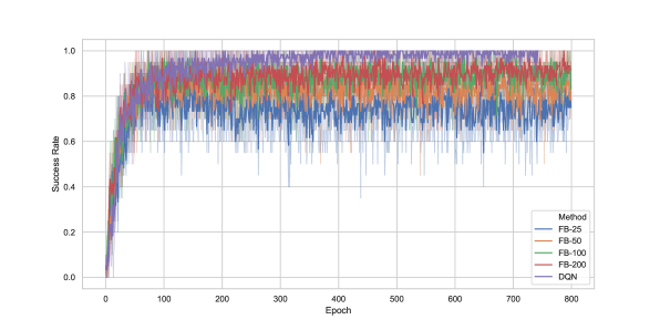
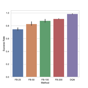
Figure 9: Continuous maze: Comparative performance of FB for different dimensions and DQN. Left: the success rate averaged over 20 randomly selected goals as function of the training epochs. Right: the success rate averaged over 1000 randomly sampled goals after 800 training epochs.

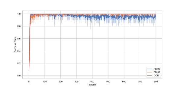
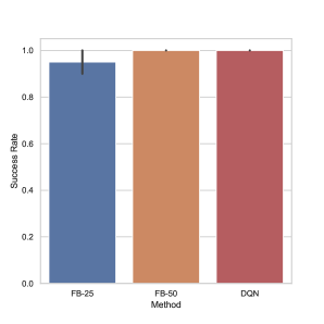
Figure 10: FetchReach: Comparative performance of FB for different dimensions and DQN. Left: the success rate averaged over 20 randomly selected goals as function of the training epochs. Right: the success rate averaged over 1000 randomly sampled goals after 800 training epochs.

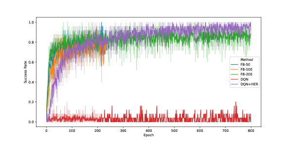
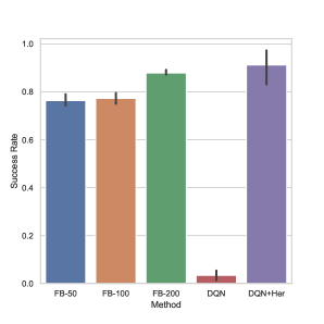
Figure 11: Ms. Pacman: Comparative performance of FB for different dimensions and DQN. Left: the success rate averaged over 20 randomly selected goals as function of the training epochs. Right: the success rate averaged over the 184 handcrafted goals after training epochs. Note that FB-50 and F-100 have been trained only for 200 epochs.

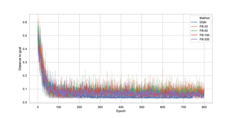
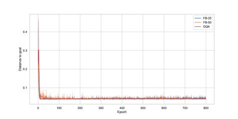
Figure 12: Distance to goal of FB for different dimensions and DQN as function of training epochs. Left: Continuous maze. Right: FetchReach.

D.4.2 More Complex Rewards: Qualitative Results

Figure 13: Discrete Maze: Heatmap plots of $\max_{a\in A}F(s,a,z_{R})^{\top}z_{R}$ (left) and trajectories of the Boltzmann policy with respect to $F(s,a,z_{R})^{\top}z_{R}$ with temperature $\tau=1$ (right). Top row: for the task of reaching a target while avoiding a forbidden region, Middle row: for the task of reaching the closest goal among two equally rewarding positions, Bottom row: choosing between a small, close reward and a large, distant one.

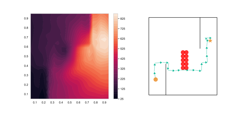
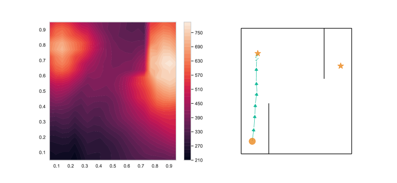
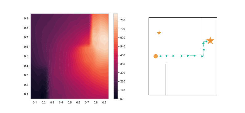
Figure 14: Continuous Maze: Contour plots plot of $\max_{a\in A}F(s,a,z_{R})^{\top}z_{R}$ (left) and trajectories of the $\varepsilon$ greedy policy with respect to $F(s,a,z_{R})^{\top}z_{R}$ with $\varepsilon=0.1$ (right). Left: for the task of reaching a target while avoiding a forbidden region, Middle: for the task of reaching the closest goal among two equally rewarding positions, Right: choosing between a small, close reward and a large, distant one..

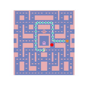
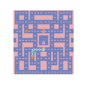
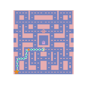
Figure 15: Ms. Pacman: Trajectories of the $\varepsilon$ greedy policy with respect to $F(s,a,z_{R})^{\top}z_{R}$ with $\varepsilon=0.1$ (right). Top row: for the task of reaching a target while avoiding a forbidden region, Middle row: for the task of reaching the closest goal among two equally rewarding positions, Bottom row: choosing between a small, close reward and a large, distant one..

D.4.3 Embedding Visualization

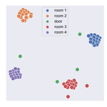
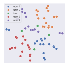
Figure 17: Discrete maze: Visualization of FB embedding vectors after projecting them in two-dimensional space with t-SNE. Left: the $F$ embedding for $z=0$. Right: the $B$ embedding. Note how both embeddings recover the foor-room and door structure of the original environment. The spread of B embedding is due to the regularization that makes B closer to orthonormal.

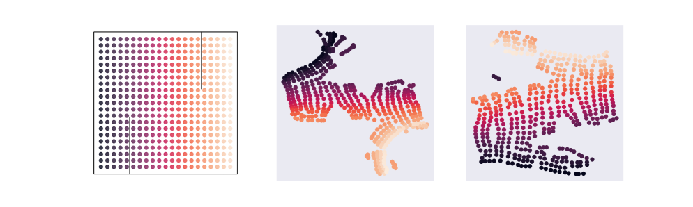
Figure 18: Continuous maze: Visualization of FB embedding vectors after projecting them in two-dimensional space with t-SNE. Left: the states to be mapped. Middle: the $F$ embedding. Right: the $B$ embedding.

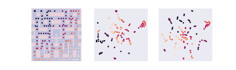
Figure 19: Ms. Pacman: Visualization of FB embedding vectors after projecting them in two-dimensional space with t-SNE. Left: the agent’s position corresponding to the state to be mapped. Middle: the $F$ embedding for $z=0$. Right: the $B$ embedding. Note how both embeddings recover the cycle structure of the environment. F acts on visual inputs and B acts on the agent’s position.

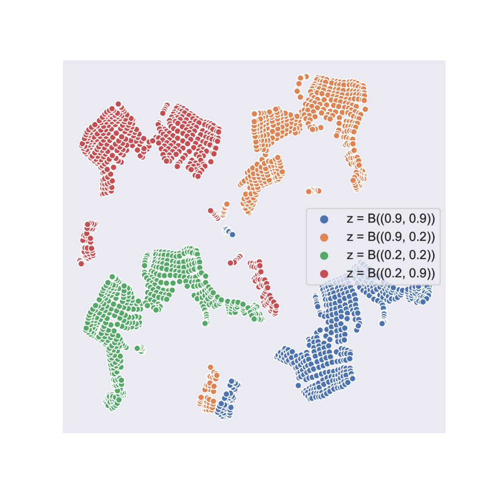
Figure 20: Continuous maze: visualization of $F$ embedding vectors for different $z$ vectors, after projecting them in two-dimensional space with t-SNE.

References

- [ACR+17] Marcin Andrychowicz, Dwight Crow, Alex Ray, Jonas Schneider, Rachel Fong, Peter Welinder, Bob McGrew, Josh Tobin, Pieter Abbeel, and Wojciech Zaremba. Hindsight experience replay. In NIPS, 2017.
- [ARO+19] Ankesh Anand, Evan Racah, Sherjil Ozair, Yoshua Bengio, Marc-Alexandre Côté, and R Devon Hjelm. Unsupervised state representation learning in atari. arXiv preprint arXiv:1906.08226, 2019.
- [BBQ+18] Diana Borsa, André Barreto, John Quan, Daniel Mankowitz, Rémi Munos, Hado van Hasselt, David Silver, and Tom Schaul. Universal successor features approximators. arXiv preprint arXiv:1812.07626, 2018.
- [BDM+17] André Barreto, Will Dabney, Rémi Munos, Jonathan J Hunt, Tom Schaul, David Silver, and Hado P van Hasselt. Successor features for transfer in reinforcement learning. In NIPS, 2017.
- [BNVB13] Marc G Bellemare, Yavar Naddaf, Joel Veness, and Michael Bowling. The arcade learning environment: An evaluation platform for general agents. Journal of Artificial Intelligence Research, 47:253–279, 2013.
- [Bog07] Vladimir I Bogachev. Measure theory. Springer, 2007.
- [Bré99] Pierre Brémaud. Markov chains: Gibbs fields, Monte Carlo simulation, and queues, volume 31. 1999.
- [BTO21] Léonard Blier, Corentin Tallec, and Yann Ollivier. Learning successor states and goal-dependent values: A mathematical viewpoint. arXiv preprint arXiv:2101.07123, 2021.
- [Day93] Peter Dayan. Improving generalization for temporal difference learning: The successor representation. Neural Computation, 5(4):613–624, 1993.
- [ESL21] Benjamin Eysenbach, Ruslan Salakhutdinov, and Sergey Levine. C-learning: Learning to achieve goals via recursive classification. In International Conference on Learning Representations, 2021.
- [FD02] David Foster and Peter Dayan. Structure in the space of value functions. Machine Learning, 49(2):325–346, 2002.
- [GHB+19] Christopher Grimm, Irina Higgins, Andre Barreto, Denis Teplyashin, Markus Wulfmeier, Tim Hertweck, Raia Hadsell, and Satinder Singh. Disentangled cumulants help successor representations transfer to new tasks. arXiv preprint arXiv:1911.10866, 2019.
- [GS97] Charles Miller Grinstead and James Laurie Snell. Introduction to probability. American Mathematical Soc., 1997.
- [HDB+19] Steven Hansen, Will Dabney, Andre Barreto, Tom Van de Wiele, David Warde-Farley, and Volodymyr Mnih. Fast task inference with variational intrinsic successor features. arXiv preprint arXiv:1906.05030, 2019.
- [JKSY20] Chi Jin, Akshay Krishnamurthy, Max Simchowitz, and Tiancheng Yu. Reward-free exploration for reinforcement learning. In International Conference on Machine Learning, pages 4870–4879. PMLR, 2020.
- [KS60] J. G. Kemeny and J. L. Snell. Finite Markov Chains. Van Nostrand, New York, 1960.
- [KST+18] Nan Rosemary Ke, Amanpreet Singh, Ahmed Touati, Anirudh Goyal, Yoshua Bengio, Devi Parikh, and Dhruv Batra. Modeling the long term future in model-based reinforcement learning. In International Conference on Learning Representations, 2018.
- [MM07] Sridhar Mahadevan and Mauro Maggioni. Proto-value functions: A Laplacian framework for learning representation and control in Markov decision processes. Journal of Machine Learning Research, 8(10), 2007.
- [PAR+18] Matthias Plappert, Marcin Andrychowicz, Alex Ray, Bob McGrew, Bowen Baker, Glenn Powell, Jonas Schneider, Josh Tobin, Maciek Chociej, Peter Welinder, et al. Multi-goal reinforcement learning: Challenging robotics environments and request for research. arXiv preprint arXiv:1802.09464, 2018.
- [RUMS18] Paulo Rauber, Avinash Ummadisingu, Filipe Mutz, and Jürgen Schmidhuber. Hindsight policy gradients. In International Conference on Learning Representations, 2018.
- [SB18] Richard S Sutton and Andrew G Barto. Reinforcement learning: An introduction. MIT press, 2018. 2nd edition.
- [SBG17] Kimberly L Stachenfeld, Matthew M Botvinick, and Samuel J Gershman. The hippocampus as a predictive map. Nature neuroscience, 20(11):1643, 2017.
- [SHGS15] Tom Schaul, Daniel Horgan, Karol Gregor, and David Silver. Universal value function approximators. In Francis Bach and David Blei, editors, Proceedings of the 32nd International Conference on Machine Learning, volume 37 of Proceedings of Machine Learning Research, pages 1312–1320, Lille, France, 07–09 Jul 2015. PMLR.
- [SMD+11] Richard S Sutton, Joseph Modayil, Michael Delp, Thomas Degris, Patrick M Pilarski, Adam White, and Doina Precup. Horde: A scalable real-time architecture for learning knowledge from unsupervised sensorimotor interaction. In The 10th International Conference on Autonomous Agents and Multiagent Systems-Volume 2, pages 761–768, 2011.
- [SPS99] Richard S Sutton, Doina Precup, and Satinder Singh. Between mdps and semi-mdps: A framework for temporal abstraction in reinforcement learning. Artificial intelligence, 112(1-2):181–211, 1999.
- [Tal17] Erik Talvitie. Self-correcting models for model-based reinforcement learning. In Proceedings of the AAAI Conference on Artificial Intelligence, volume 31, 2017.
- [VdMH08] Laurens Van der Maaten and Geoffrey Hinton. Visualizing data using t-sne. Journal of machine learning research, 9(11), 2008.
- [ZSBB17] Jingwei Zhang, Jost Tobias Springenberg, Joschka Boedecker, and Wolfram Burgard. Deep reinforcement learning with successor features for navigation across similar environments. In 2017 IEEE/RSJ International Conference on Intelligent Robots and Systems (IROS), pages 2371–2378. IEEE, 2017.