Semi-Supervised Video Deraining with Dynamical Rain Generator

Abstract

While deep learning (DL)-based video deraining methods have achieved significant successes in recent years, they still have two major drawbacks. Firstly, most of them are insufficient to model the characteristics of rain layers contained in rainy videos. In fact, the rain layers exhibit strong visual properties (e.g., direction, scale, and thickness) in spatial dimension and causal properties (e.g., velocity and acceleration) in temporal dimension, and thus can be modeled by the spatial-temporal process in statistics. Secondly, current DL-based methods rely heavily on the labeled training data, whose rain layers are synthetic, thus leading to a deviation from real data. Such a gap between synthetic and real data sets results in poor performance when applying them to real scenarios. To address these issues, this paper proposes a new semi-supervised video deraining method, in which a dynamical rain generator is employed to fit the rain layer for the sake of better depicting its intrinsic characteristics. Specifically, the dynamical generator consists of one emission model and one transition model to simultaneously encode the spatial appearance and temporal dynamics of rain streaks, respectively, both of which are parameterized by deep neural networks (DNNs). Furthermore, different prior formats are designed for the labeled synthetic and unlabeled real data so as to fully exploit their underlying common knowledge. Last but not least, we design a Monte Carlo-based EM algorithm to learn the model. Extensive experiments are conducted to verify the superiority of the proposed semi-supervised deraining model.

1 Introduction

Rain is a very common bad weather that exists in many videos. The appearance of rain not only negatively affects the visual quality of the video, but also seriously deteriorates the performance of subsequent video processing algorithms, e.g., semantic segmentation[38], object detection[9], and autonomous driving[7]. Thus, as a necessary video pre-processing step, video deraining has attracted much attentions from the computer vision community.

As an ill-posed inverse problem raised by Garg and Nayar[15], various methods have been proposed to handle the video deraining task[47]. Most of the traditional methods focus on exploiting rational prior knowledge for the background or rain layers so as to obtain a proper separation between them. For example, low-rankness[23, 53, 24] is widely used to encode the temporal correlations of background video. As for rain streaks, many visual characteristics, such as photometric appearance[16], geometrical features[41], chromatic consistency[36], local structure correlations[8] and multi-scale convolutional sparse coding[31], have been explored in the past few years. Different from these deterministic assumptions for rain streaks, Wei et al.[53] firstly regard them as random variables, and use Gaussian mixture model (GMM) to fit them. Albeit substantiated to be effective in some ideal scenarios, these traditional methods are mainly limited by the subjective manually-designed prior knowledge and huge computation burden.

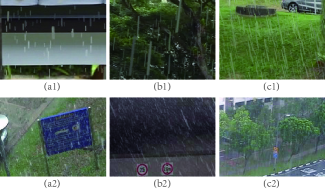
Figure 1: The comparison of typical synthetic and real rainy images in NTURain data set. (a1)-(c1): synthetic rainy images, (a2)-(c2): real rainy images.

Recently, owning to the powerful nonlinear fitting capability of DNNs, DL-based methods facilitate significant improvements for the video deraining task. The core idea of this methodology is to directly train a derainer parameterized by DNNs based on synthetic rainy/clean video pairs in an end-to-end manner. Most of these methods leverage different technologies, e.g., superpixel alignment[6], dual-level flow[56] and self-learning[58], to extract clean backgrounds from rainy videos. In addition, Liu et al.[35, 34] design a recurrent network to jointly perform both the rain degradation classification and rain removal tasks.

Even though these DL-based methods have achieved impressive deraining results on some synthetic benchmarks, there still exists large room to further increase the performance and the generalization capability in real applications. On one hand, most of these methods make efforts to depict the background, but neglect to model the intrinsic characteristics of the rain layers. In fact, the rain layer in video, which is an image sequence of rain steaks, can be represented by a spatial-temporal process. Specifically, the randomly scattered rain streaks in each time frame are characterized with evident visual properties (e.g., direction, scale, and thickness) in the spatial dimension, and the rain layers in different time frames correspond to a continuous time series along the temporal dimension, showing the causal properties (e.g., velocity and acceleration) of the rain dynamics. Therefore, elaborately representing and exploiting these intrinsic physical properties underlying the rain layers in video data is expected to facilitate the rain removal task.

On the other hand, it is well known that the performance of DL-based methods heavily relies on a large amount of pre-collected training data, i.e., rainy/clean video pairs. In fact, due to the high labor cost to obtain such video pairs in real scenes, most of current methods have to use synthetic ones, which are manually simulated based on the photo-realistic rendering technique [17] or professional photography and human supervision [50]. Fig.1 presents several typical frames of synthetic and real rainy images in NTURain [6] data set, which is widely used as a benchmark for current video deraining methods. It can be easily seen that the rain patterns in synthetic and real rainy images are obviously different, and the real ones contain more complex and diverse rain types. Because of such a deviation between synthetic and real data sets, the performances of these DL-based methods deteriorate seriously in the real cases. To deal with the generic video deraining task, it is thus critical to build a reasonable semi-supervised learning framework that sufficiently exploits the common knowledge in the labeled synthetic and unlabeled real data.

To address these issues, in this paper we propose a semi-supervised video deraining method, in which a dynamical rain generator is adopted to mimic the generation process of the rain layers in video, hopefully better capturing the intrinsic knowledge simultaneously from the spatial and temporal dimensions. Besides, the real rainy videos are taken into consideration in our model as unlabeled data, in order to achieve more robust deraining results. In summary, the contributions of this work are as follows:

Firstly, we propose a new probabilistic video deraining method, in which a dynamical rain generator, consisting of a transition model and an emission model, is employed to fit the rain layers in videos. Specifically, the transition model is used to represent the dynamics of rains in a low-dimensional state space, while the emission model seeks to generate the observed rain streaks in the image space from the state space. To increase the capacities of such a dynamical rain generator, both the transition and emission models are parameterized by DNNs. Secondly, a semi-supervised learning mechanism is designed by constructing different prior formats for labeled synthetic data and unlabeled real data. Specifically, for the labeled synthetic data, the corresponding ground truth rain-free videos are included into an elaborate prior distribution as a strong constraint. As for the unlabeled real data, we introduce the 3-D Markov Random Field (MRF) to model the temporal consistencies and correlations of the underlying backgrounds. Thirdly, a Monte Carlo-based EM algorithm is designed to learn the model. In the expectation step, the posterior of the latent variables is intractable due to the usages of DNNs to parameterize the generator and derainer, thus the Langevin dynamics is adopted to approximate the expectation.

2 Related Work

In this section, we give a short recap for the developments on the video/image deraining methods.

2.1 Video Deraining Methods

To the best of our knowledge, Garg and Nayar[15] firstly proposed the problem of video deraining, and developed a rain detector based on the photometric appearance of rain. Later, they further explored the relationships between rain effects and some camera parameters [16, 17, 18].

Inspired by these seminal works, various video deraining methods have been proposed in the past few years, focusing on seeking more reasonable prior knowledge for the rain or background. For example, both the chromatic properties [64, 36] and shape characteristics [3, 2] of rain in the time domain were employed to identify and remove the rain layers from the captured rainy videos, while the regular visual effects of rain in the global frequency space were also exploited by [1]. Besides, Santhaseelan and Asari [43] employed local phase congruency to detect rain based on chromatic constraints. Notably, Wei et al.[53] firstly regarded rain streaks as random variables and fitted them by GMM. In addition, matrix/tensor factorization technologies were also very popular in the field of video deraining, which were typically used to encode the correlations of background video along the temporal dimension, e.g.,  [8, 27, 23, 24, 41].

In recent years, DL-based methods represent a new trend along this research line. In [31], Li et al. employed the multi-scale convolutional sparse coding to encode the repetitive local patterns under different scales of rain streaks. Chen et al. [6] proposed to decompose the scene into superpixels and then align the scene content based on the superpixel segmentation result, and finally a CNN was used to compensate the lost details and add normal textures to the deraining result. In [35], Liu et al. designed a recurrent neural network to jointly perform the rain degradation classification and rain removal tasks. And in [34], a hybrid rain model was proposed to model both rain streaks and occlusions. Besides, Yang et al.[56] also built a two-stage recurrent networks that utlize dual-level regularizations toward video deraining. Very recently, Yang et al. [58] proposed a self-learning manner for this task by taking both temporal correlations and consistencies into consideration.

While DL-based methods have achieved impressive performance on some synthetic benchmarks, they are still very hard to be applied to the real applications due to the large gap between the used synthetic data and the real data. Therefore, in order to increase the generalization capacity of the deraining model in the real tasks, it is crucial to design a semi-supervised learning framework that makes use of the information in both the labeled synthetic data and the unlabeled real one. This paper mainly focuses on this issue.

2.2 Single Image Deraining Methods

For literature comprehensiveness, we also briefly review the single image deraining methods. The single image deraining method can be roughly divided into two categories, i.e., model-based methods and DL-based methods. Most of the model-based methods formulate the deraining task as a decomposition problem of the rain and background layers, and various technologies have been employed to deal with it, such as morphological component analysis [25], non-local means filter [26], and sparse coding [5, 37]. Besides, methods built on prior knowledge of rain and background are also explored in this field, mainly including sparsity and low-rankness [60, 4, 19], narrow directions of rain and the similarities of rain patches [66], and GMM [33].

The earliest DL-based method was proposed by Fu et al. [12, 13], in which CNNs were adopted to remove rains from the high frequency parts of rainy images. Led by these two works, DL-based methods began to dominate the research in this field. Many effective and advanced network architectures [30, 32, 40, 50, 14, 21] were put forward in recent years. And some works attempted to jointly handle the rain removal task with other related tasks, e.g., rain detection [57], rain density estimation [61], so as to obtain better deraining performance. Besides, some useful priors, e.g., multi-scale [59, 65, 22], convolutional sparse coding [48] and bilevel layer prior [39], were also embedded into the DL-based methods to sufficiently mine the potentials of DNNs. Different from the above methods, Zhang et al. [62] and Wang et al. [46] both introduced the adversarial learning scheme to enhance the fidelity of the derained images, and Wei et al. [52] proposed a semi-supervised deraining model that can be better generalized to real tasks.

In general, single image deraining methods can be directly used in the video deraining task by treating each video as a bunch of independent images. However, ignoring the abundant temporal information contained in videos will lead to an unsatisfied performance. Thus it is necessary to design a reasonable deraining model specific for video data.

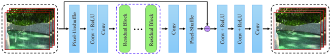
Figure 2: The network architecture for the derainer $f(\cdot;W)$. In this figure, all “Conv”s denote the 3-D convolution layer.

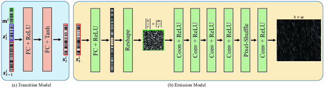
Figure 3: An illustration of network architectures of the transition model and the emission model in the dynamical rain generator. In this figure, “FC”, “Conv” and “Tanh” denote fully connected, 2-D convolution and hyperbolic tangent layers, respectively. “Pixel-Shuffle” is the sub-pixel layer [45] with a scale factor $r$.

3 Semi-Supervised Video Deraining Model

Given a labeled data set $\mathcal{D}=\{\mathcal{Y}^{k},\mathcal{X}^{k}\}_{k=1}^{N_{l}}$ and an unlabeled data set $\mathcal{U}=\{\mathcal{Y}^{k}\}_{k=1}^{N_{u}}$, where $\mathcal{Y}^{k}$ and $\mathcal{X}^{k}$ denote the $k$-th rainy and clean videos, respectively, we aim to construct a semi-supervised probabilistic model based on them and then design an EM algorithm to learn the model.

3.1 Model Formulation

Let $\mathcal{Y}=\{\mathcal{Y}_{t}\}_{t=1}^{n}$ denote any rainy video in $\mathcal{D}$ or $\mathcal{U}$, where $\mathcal{Y}_{t}\in\mathcal{R}^{h\times w}$ is the $t$-th image frame. Similar to [31, 33], we decompose the rainy video $\mathcal{Y}$ into three parts, i.e.,

$$\mathcal{Y}=f(\mathcal{Y};W)+\mathcal{R}+\mathcal{E},~{}~{}\mathcal{E}_{ijt}\sim\mathcal{N}(0,\sigma^{2}),$$ (1)

where $f(\mathcal{Y};W)$, $\mathcal{R}$ and $\mathcal{E}$ are the recovered rain-free background, rain layer and residual term, respectively, and $\mathcal{E}_{ijt}$ is the element of $\mathcal{E}$ at location $(i,j,t)$. The residual term is assumed to follow a zero-mean Gaussian distribution with variance $\sigma^{2}$. $f(\cdot;W)$, which is parameterized by DNNs, denotes a function that maps the observed rainy video to the underlying rain-free background, and is called the “derainer” in this paper. Next, we consider how to model the derainer parameter $W$ and rain layer $\mathcal{R}$:

Modeling of background layer: As is well known, one general prior knowledge for video data is that the rain-free background video has strong correlations and similarities along spatial and temporal dimensions. Therefore, for any rainy video $\mathcal{Y}\in\mathcal{U}$, we encode such a knowledge through the following MRF prior distribution for $W$:

$$p(W)\propto\exp\left(-\rho\sum_{i,j,t}\bm{v}^{T}\bm{\gamma}\right),$$ (2)

where $\bm{v}=\left[\begin{smallmatrix}|f_{i+1,j,t}-f_{ijt}|\\ |f_{i,j+1,t}-f_{ijt}|\\ |f_{i,j,t+1}-f_{ijt}|\end{smallmatrix}\right]$, $\bm{\gamma}=\left[\begin{smallmatrix}\gamma_{1}\\ \gamma_{2}\\ \gamma_{3}\end{smallmatrix}\right]$, and $f_{ijt}$ denotes the element of $f(\mathcal{Y};W)$ at location $(i,j,t)$. $\rho$ and $\bm{\gamma}$ are both manual hyper-paramerters, and the latter represents the strength of smoothness constraint on the spatial and temporal dimensions. As for the rainy video $\mathcal{Y}\in\mathcal{D}$, the known rain-free background $\mathcal{X}$ can be further embedded into Eq. (2) as another strong prior, i.e.,

$$p(W)\propto\exp\left(-\frac{\|f(\mathcal{Y};W)-\mathcal{X}\|_{2}}{\varepsilon_{0}^{2}}-\rho\sum_{i,j,t}\bm{v}^{T}\bm{\gamma}\right),$$ (3)

where $\varepsilon_{0}$ is a very small hyper-paramerter close to zero.

As for the derainer $f(\cdot;W)$, we adopt a simple network architecture as shown in Fig. 2. Without any special designs, it only contains several 3-D convolution layers and residual blocks [20]. To accelerate the computation, the pixel-unshuffle [63] and pixel-shuffle [45] layers are added to the head and the tail of the network, respectively.

Modeling of rain layer: Intuitively, the rain layer is a dynamical sequence, thus we naturally employ the spatial-temporal process [11, 55, 54] in statistics to characterize it. Let’s use $\mathcal{R}_{t}$ to denote the $t$-th image frame of rain layer sequence $\mathcal{R}$, and then our dynamical rain generator can be formulated as follows,

$$\bm{s}_{t} =F(\bm{s}_{t-1},\bm{z}_{t};\bm{\alpha}),$$ (4)

$$\mathcal{R}_{t} =H(\bm{s}_{t};\bm{\beta}),$$ (5)

where

$$\bm{z}_{t}\sim\mathcal{N}(0,\bm{I}),~{}\bm{s}_{0}\sim\mathcal{N}(0,\bm{I}),$$ (6)

$\bm{s}_{t}$ represents the hidden state variable in $t$-th frame, and $\bm{z}_{t}$ the noise vector. Specifically, Eq. (4) is the transition model with parameters $\bm{\alpha}$ expecting to depict the dynamics of rains over time, and Eq. (5) is the emission model with parameters $\bm{\beta}$ that maps the hidden state space to the space of rain layer. Note that the noise vectors $\{\bm{z}_{t}\}_{t=1}^{n}$ are independent of each other, and each $z_{t}$ encodes the random factors that affect the rains (e.g., wind, camera motion, etc) at time $t$ in the transition from $\bm{s}_{t-1}$ to $\bm{s}_{t}$.

Furthermore, following [55], we can extend the generator to an advanced version for multiple rain videos. Specifically, for the $i$-th rain video $\mathcal{R}^{i}=\{\mathcal{R}_{t}^{i}\}_{t=1}^{n}$, another vector $\bm{m}^{i}\sim\mathcal{N}(0,\bm{I})$ is introduced to account for the variation of rain appearances or patterns over different videos, and thus the transition model of Eq. (4) can be reformulated as:

$$\bm{s}_{t}^{i}=F(\bm{s}_{t-1}^{i},\bm{z}_{t}^{i},\bm{m}^{i};\bm{\alpha}),$$ (7)

where $\bm{m}^{i}$ is fixed for the $i$-th rain video. For notation convenience, we write Eqs. (7) and (5) together as follows:

$$\mathcal{R}^{i}=G(\bm{s}^{i}_{0},\bm{z}^{i},\bm{m}^{i};\bm{\theta}),$$ (8)

where $\bm{z}^{i}=\{\bm{z}^{i}_{t}\}_{t=1}^{n}$, $\bm{\theta}=\{\bm{\alpha},\bm{\beta}\}$. In practice, we use the extended version of Eq. (8) to simultaneously fit the rain layers in each mini-batch of video data.

To increase the capacity of such a dynamical rain generator, we parameterize both of the transition model and the emission model by DNNs. Following [55], we use a two-layers mutli-layer perceptron (MLP) in Fig. 3 (a) for the transition model. As to the emission model, we elaborately design a CNN architecture that takes the state variable $\bm{s}_{t}$ as input and outputs the rain image as shown in Fig. 3 (b), which is mainly inspired by a recent work [49] that uses CNN as a latent variable model to generate rain streaks.

Remark: The employment of such a dynamical generator to fit the rain layers is one of the main contributions of this work, which directly affects the deraining performance of the entire model. Therefore, it is necessary to validate the capability of the dynamical generator on simulating the rain layers. To prove this point, we pre-collected some rain layer videos synthesized by commercial Adobe After Effects software from YouTube as source videos, and trained the dynamical generator on them. Empirically, we found that the proposed dynamical rain generator is able to sufficiently mimic the given rain layer videos. Due to the page limitation, we put the experiments to the supplementary materials.

3.2 Maximum A Posteriori Estimation

Combining Eqs. (1)-(6), a full probabilistic model is obtained for video deraining. Then our goal turns to maximize the posteriors w.r.t the model parameters $W$ and $\bm{\theta}$, i.e.,

$$\max_{W,\bm{\theta}}\log p(W,\bm{\theta}|\mathcal{Y}) =\log p(\mathcal{Y}|W,\bm{\theta})+\log p(W)+\text{const}$$

$$\triangleq\mathcal{L}(\mathcal{Y};W,\bm{\theta}),$$ (9)

where $p(\mathcal{Y}|W,\bm{\theta})$ is the likelihood of the rainy video $\mathcal{Y}$. According to Eqs. (1) and (8), it can be written as:

$$p(\mathcal{Y}|W,\bm{\theta}) =\int p(\mathcal{Y}|W,\bm{\theta},\bm{z})p(\bm{z})\operatorname{d\!}\bm{z}$$

$$=\int\mathcal{N}\left(f(\mathcal{Y};W)+G(\bm{s}_{0},\bm{z};\bm{\theta}),\sigma^{2}\bm{I}\right)p(\bm{z})\operatorname{d\!}\bm{z}.$$

Finally, we directly optimize the problem of Eq. (9) on the whole labeled and unlabeled data sets, i.e.,

$$\max_{W,\bm{\theta}}\sum\limits_{\mathcal{Y}^{k}\in\mathcal{D}}\mathcal{L}(\mathcal{Y}^{k};W,\bm{\theta})+\sum\limits_{\mathcal{Y}^{k}\in\mathcal{U}}\mathcal{L}(\mathcal{Y}^{k};W,\bm{\theta}).$$ (10)

The insight behind Eq. (10) is to learn a general mapping from rainy videos to clean ones, based on large amount of data samples in $\mathcal{D}$ and $\mathcal{U}$, which is expected to obtain a more efficient and robust derainer than that in traditional inference paradigm implementing on single video.

Most notably, if only considering labeled data set, our method naturally degenerates into a supervised deraining model. However, involving the unlabeled real data can increase the generalization capacity of the model such that it can be applied to the real cases as shown in the ablation studies in Sec. 4.2.2.

3.3 Inference and Learning Algorithm

For notation brevity, we only consider one data sample $\mathcal{Y}$ in this part. Inspired by the technology of alternative back-propagation through time [55], a Monte Carlo-based EM [10] algorithm is designed to maximize $\mathcal{L}(\mathcal{Y};W,\bm{\theta})$, in which the expectation step samples the latent variable $\bm{z}$ from the posterior distribution $p(\bm{z}|\mathcal{Y})$, and the maximization step updates the model parameters $W$ and $\bm{\theta}$ based on the inferred latent variable $\bm{z}$.

E-Step: Let $(W^{\text{old}},\bm{\theta}^{\text{old}})$ and $p_{\text{old}}(\bm{z}|\mathcal{Y})$ denote the current model parameters and the posterior under them, we can sample $\bm{z}$ from $p_{\text{old}}(\bm{z}|\mathcal{Y})$ using the Langevin dynamics [29]:

$$\bm{z}^{(\tau+1)} =\bm{z}^{(\tau)}+\frac{\delta^{2}}{2}\left[\frac{\partial}{\partial\bm{z}}\log p_{\text{old}}(\bm{z}|\mathcal{Y})\right]\bigg{|}_{\bm{z}=\bm{z}^{(\tau)}}+\delta\bm{\xi}^{(\tau)}$$

$$=\bm{z}^{(\tau)}-\frac{\delta^{2}}{2}\left[\frac{\partial}{\partial\bm{z}}g(\bm{z})\right]\bigg{|}_{\bm{z}=\bm{z}^{(\tau)}}+\delta\bm{\xi}^{(\tau)}$$ (11)

where we define

$$g(\bm{z})=\frac{1}{2\sigma^{2}}\left\|\mathcal{Y}-f(\mathcal{Y};W^{\text{old}})-G(\bm{s}^{0},\bm{z};\bm{\theta}^{\text{old}})\right\|_{2}+\frac{1}{2}\|\bm{z}\|_{2},$$ (12)

$\tau$ indexs the time step for Langevin dynamics, $\delta$ denotes the step size, and $\bm{\xi}^{(\tau)}$ is the Gaussian white noise, which is used to avoid falling into local modes. A key point to compute Eq. (11) is $\frac{\partial}{\partial\bm{z}}\log p_{\text{old}}(\bm{z}|\mathcal{Y})=\frac{\partial}{\partial\bm{z}}\log p_{\text{old}}(\mathcal{Y},\bm{z})$, and the right term can be easily calculated.

Algorithm 1 Inference and learning procedure for S2VD

0:  training data $\mathcal{D}=\{\mathcal{Y}^{b_{j}},\mathcal{X}^{b_{j}}\}_{j=1}^{B_{l}}$ and $\mathcal{U}=\{\mathcal{Y}^{b_{j}}\}_{j=B_{l}+1}^{B_{l}+B_{u}}$, where $\mathcal{Y}^{b_{j}}$ denotes the $j$-th mini-batch data, number of Langevin steps $l$.

0:  the derainer parameters $W$.

1:  Initialize $W$ and $\bm{\theta}^{b_{j}}$, $\bm{z}^{b_{j}}$, $j=1,2,\cdots,B_{l}+B_{u}$.

2:  while not converged do

3:     for $j=1,2,\cdots,B_{l}+B_{u}$ do

4:        Sample the mini-batch data $\{\mathcal{Y}^{b_{j}},\mathcal{X}^{b_{j}}\}$ or $\mathcal{Y}^{b_{j}}$.

5:        E-Step: For each data example $\mathcal{Y}^{i}$ in current mini-batch $\mathcal{Y}^{b_{j}}$, run $l$ steps of Langevin dynamics to sample $\bm{z}^{i}$ following Eq. (12).

6:        M-Step: Update $W$ and $\bm{\theta}^{b_{j}}$ by Eq. (15).

7:     end for

8:  end while

In practice, for the purpose of avoiding the high computational cost of MCMC, At each learning iteration, Eq. (11) starts from the previous updated results of $\bm{z}$. As for the initial state vector $\bm{s}_{0}$ and the rain variation vector $\bm{m}$ in Eq. (8), because they are also latent variables in our model, we sample them together with $\bm{z}$ using the Langevin dynamics.

Table 1: PSNR/SSIM results of different methods on the synthetic testing data set of NTURain. The best and second best results are highlighted in red and blue, respectively.

Clip No.	Rain		DSC [37]		FastDerain [24]		DDN [13]		PReNet [40]		SpacCNN [6]		SLDNet [58]		S2VD
17
	PSNR	SSIM	PSNR	SSIM	PSNR	SSIM	PSNR	SSIM	PSNR	SSIM	PSNR	SSIM	PSNR	SSIM	PSNR	SSIM
a1	29.71	0.9149	27.15	0.9079	29.29	0.9159	31.79	0.9481	32.13	0.9511	30.57	0.9334	33.72	0.9508	36.39	0.9658
a2	29.30	0.9284	28.84	0.9224	30.21	0.9245	30.34	0.9360	30.41	0.9375	31.29	0.9356	33.82	0.9512	33.06	0.9519
a3	29.08	0.8964	26.73	0.8942	29.94	0.9039	30.70	0.9301	30.73	0.9316	30.63	0.9247	33.12	0.9404	35.75	0.9564
a4	32.62	0.9381	30.58	0.9381	34.69	0.9707	35.77	0.9689	35.77	0.9700	35.30	0.9620	37.35	0.9722	39.53	0.9779
b1	30.03	0.8956	30.06	0.9015	29.35	0.9139	32.53	0.9465	32.66	0.9491	32.26	0.9454	34.21	0.9482	37.34	0.9712
b2	30.69	0.8874	30.85	0.9017	31.90	0.9520	33.89	0.9559	33.74	0.9557	35.11	0.9677	35.80	0.9595	40.55	0.9821
b3	32.31	0.9299	31.30	0.9295	29.28	0.9287	35.38	0.9663	35.34	0.9681	34.69	0.9566	36.34	0.9614	38.82	0.9754
b4	29.41	0.8933	30.61	0.9089	27.70	0.9095	32.62	0.9462	33.17	0.9526	34.87	0.9536	33.85	0.9469	37.53	0.9657
avg.	30.41	0.9108	29.52	0.9130	30.54	0.9255	32.87	0.9497	32.99	0.9519	33.11	0.9475	34.89	0.9540	37.37	0.9683

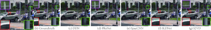
Figure 4: Qualitative results of different methods on one typical image in NTURain synthetic testing data set. From left to right: (a) rainy image, (b) ground truth image, (c)-(g) deraining results by DDN, PReNet, SpacCNN, SLDNet and our S2VD.

M-Step: Denote the sampled latent variable in E-Step as $\tilde{\bm{z}}$, M-Step aims to maximize the approximate lower bound w.r.t. $W$ and $\bm{\theta}$ as follows:

$$\max_{W,\bm{\theta}}\mathcal{Q}(W,\bm{\theta}) =\int p_{\text{old}}(\bm{z}|\mathcal{Y})\log p(\mathcal{Y},\bm{z}|W,\bm{\theta})\operatorname{d\!}\bm{z}+\log p(W)$$

$$\approx\log p(\mathcal{Y},\tilde{\bm{z}}|W,\bm{\theta})+\log p(W).$$ (13)

Equivalently, Eq. (13) can be further rewritten as the following minimization problem, i.e.,

$$\min_{W,\bm{\theta}}\hat{\mathcal{L}}(W,\bm{\theta}) =\frac{1}{2\sigma^{2}}\left\|\mathcal{Y}-f(\mathcal{Y};W)-G(\tilde{\bm{z}},\bm{s}^{0};\bm{\theta})\right\|_{2}+$$

$$\mathrel{\phantom{=}}\rho\sum_{i,j,t}\bm{v}^{T}\bm{\gamma}+1_{[\mathcal{Y}\in\mathcal{D}]}\cdot\frac{\|f(\mathcal{Y};W)-\mathcal{X}\|_{2}}{\varepsilon_{0}^{2}},$$ (14)

where $1_{[\mathcal{Y}\in\mathcal{D}]}$ equals to 1 when $\mathcal{Y}$ comes from the labeled data set $\mathcal{D}$ otherwise 0. Naturally, we can update $W$ and $\bm{\theta}$ by gradient descent based on the back-propagation (BP) algorithm [42] as follows,

$$\varLambda\leftarrow\varLambda-\eta\frac{\partial}{\partial\varLambda}\hat{\mathcal{L}}(W,\bm{\theta}),~{}\varLambda\in\{W,\bm{\theta}\},$$ (15)

where $\eta$ denotes the step size.

Due to the capacity limitation, we empirically find it difficult to fit the rain layers in all training videos using only one single generator defined in Eq. (8). Therefore, we train one generator for each mini-batch data. With such a strategy, our model performs well throughout all our experiments. The mini-batch size is 12. A detailed description of the proposed algorithm is presented in Algorithm 1.

4 Experimental Results

In this section, we conduct some experiments to evaluate the effectiveness of the proposed semi-supervised video deraining model on synthetic and real data sets. And we briefly denote our Semi-Supervised Video Deraining model by S2VD in the following presentation.

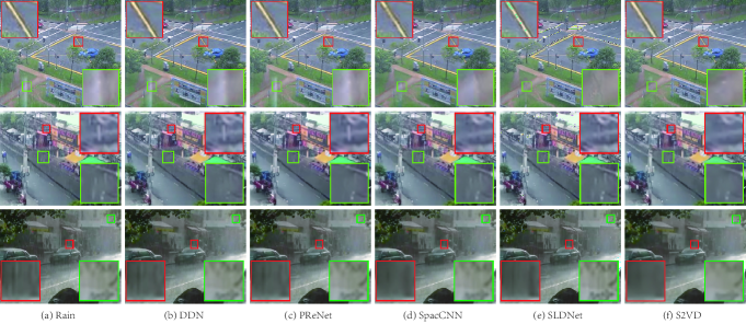
Figure 5: Visual comparisons of different methods on three typical real testing images from NTURain [6] (the 1st row) and [31] (the 2nd and 3rd row). From left to right: (a) rainy image, (b)-(f) deraining results by DDN, PReNet, SpacCNN, SLDNet and our S2VD.

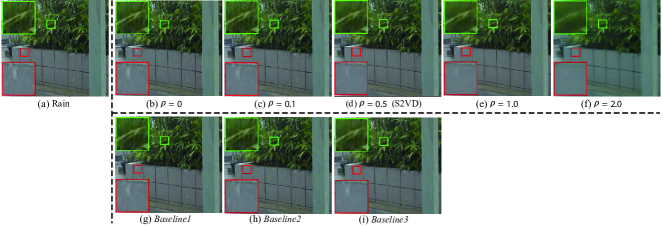
Figure 6: Comparisons of S2VD under different settings: (a) rainy image, (b)-(f) deraining results of S2VD with different $\rho$ values, (g)-(i) deraining results of different Baselines defined in Sec. 4.2.2.

4.1 Evaluation on Rain Removal Task

Training Details: To train S2VD, we employ the synthesized training data of NTURain [6] as labeled data set, which contains 8 rain-free video clips of various scenes. For each rain-free video, 3 or 4 rain layers are synthesized by the Adobe After Effects with different settings, and then added to the videos as rainy ones. As for unlabeled data, 7 real rainy videos without ground truths in the testing data of NTURain are employed. To relieve the burden of GPU memory, we use truncated back-propagation through time in training, meaning that the whole training sequence is divided into different non-overlapped chunks for forward and backward propagation. The length of each chunk is 20.

The Adam [28] algorithm is used to optimize the model parameters in the M-Step of our algorithm. All the network parameters are initialized by [44]. The initialized learning rates for the transition model, emission model and the derainer are set to be $1e\text{-}3$, $1e\text{-}4$ and $2e\text{-}4$, respectively, and decayed by half after 30 epochs. The mini-batch size is set as 12, and each video is clipped into small blocks with spatial size $64\times 64$ pixels. Note that we only update the parameter $W$ for the first 5 epochs to pretrain the derainer, which makes the training more stable. As for the hyper-parameters, $\varepsilon_{0}^{2}=1e\text{-}6$, $\rho=0.5$, $\bm{\gamma}=[1,1,2]^{T}$, and more analysis experiments on them are presented in Sec. 4.2.

4.1.1 Evaluation on Synthetic Data

We test our S2VD on the synthetic testing data set of NTURain [6], which consists of two groups of data sets. The videos in the first group (with prefix “a” in Table 1) are captured by a panning and unstable camera, while those in the second group (with prefix “b” in Table 1) by a fast moving camera with a speed range from 20 to 30 km/h. As to the methods for comparison, six SOTAs are considered, including one model-based image deraining method DSC [37], one model-based video deraining method FastDerain [24], two DL-based image deraining methods DDN [13] and PReNet [40], two DL-based video deraining methods SpacCNN [6] and SLDNet [58]. The average PSNR and SSIM [51] are used as quantitative metrics, which are evaluated only in the luminance channel since we are sensitive to the luminance information.

Table 2: Average PSNR/SSIM results of S2VD on the synthetic testing dataset of NTURain under different $\rho$ values.

Metrics	$\rho$
6
	0	0.1	0.5	1	2
PSNR	38.18	38.05	37.37	35.50	31.55
SSIM	0.9719	0.9713	0.9683	0.9519	0.8947

Table 1 lists the average PSNR/SSIM results on 8 testing videos. Evidently, S2VD attains the best or at least second best performance in all cases. Comparing with current SOTAs (SpacCNN or SLDNet), our method achieves at least 2.5dB PSNR and 0.01 SSIM gains. The qualitative results are shown in Fig. 4. Note that we only display the results of DL-based methods due to the page limitation. We observe that: 1) The derained results of PReNet still contain some rain streaks. 2) Both DDN and SpacCNN lose some image contents. 3) SLDNet can not preserve the original color maps very well. However, our S2VD evidently alleviate these deficiencies and obtains the closest results to the ground truths, which verifies the effectiveness of our model.

Table 3: Average PSNR/SSIM results of three baselines and S2VD on the synthetic testing dataset of NTURain.

Metrics	Methods
5
	Baseline1	Baseline2	Baseline3	S2VD
PSNR	36.11	37.12	37.96	37.37
SSIM	0.9602	0.9673	0.9717	0.9683

4.1.2 Evaluation on Real Data

To further test the generalization capability of S2VD in real tasks, we evaluate it on two kinds of real rainy videos, i.e., the real testing data set in NTURain and several other real rainy videos in  [31]. Note that the former is included in our training set as unlabeled data, but the latter is not. Fig. 5 presents some typical deraining results by different methods on these two kinds of data sets. It can be seen that S2VD achieves the best visual results comparing with other methods. Especially, the superiority of our model shown in the second data set substantiates that S2VD is able to handle the real rainy videos even though they do not appear in the unlabeled data set. This generalization capability would be potentially useful in real deraining tasks.

4.2 Additional Analysis

4.2.1 Sensitiveness of Hyper-paramerter $\rho$

The hyper-paramerter $\rho$ in Eq. (2) or (3) controls the relative importantance of MRF prior in S2VD. The quantitative performances on the synthetic testing data set and the qualitative performances on the real testing data set of NTURain under different $\rho$ values are presented in Table 2 and Fig. 6, respectively. On one hand, when $\rho$ increases, the performance on the synthetic testing set tends to decrease as shown in Table 2, since the relative importance of the constraint built on the ground truth in Eq. (3) decreases. On the other hand, the MRF prior is able to prevent the derainer from overfitting the synthetic data, thus improving the generalization capability in real cases, which has been sufficiently verified by the visual comparisons in Fig. 6. By taking into account these two aspects, we set $\rho$ as $0.5$.

4.2.2 Ablation Studies

As shown in Eq. (14), our S2VD degenerates into the Mean Squre Error (MSE) loss when $\varepsilon_{0}\rightarrow 0$. Comparing with such special case, our model introduces one more likelihood term, one more MRF regularizer and the semi-supervised learning paradigm. To clarify the effect of each part, we compare S2VD with three baselines as follows: 1) Baseline1: We only train the derainer with the MSE loss on labeled data set. 2) Baseline2: We train S2VD with $\varepsilon_{0}^{2}=1e\textit{-}6$ and $\rho=0$ only on labeled data set so that we can justify the marginal gain from the likelihood term by comparing with Baseline1 using the MSE loss. 3) Baseline3: On the basis of Baseline2, we introduce the MRF regularizer with $\rho=0.5$.

The quantitative comparisons on synthetic testing data set of NTURain are listed in Table 3, and the visual results on real testing data set are also displayed in Fig. 6. In summary, we can see that: 1) The performance improvement (1.01dB PSNR and 0.0071 SSIM) of Baseline2 beyond Baseline1 substantiates that the likelihood term plays an important role in our model. 2) Under the supervised learning manner, the MRF prior is beneficial to our model in both synthetic and real cases according to the performance of Baseline3. 3) The addition of unlabeled data in S2VD increases the generalization capability in real tasks as shown in Fig. 6 (d) and (i). However, it leads to a little deterioration of the performance on synthetic data, mainly because there is a gap between the rain types contained in the labeled synthetic and unlabeled real data sets.

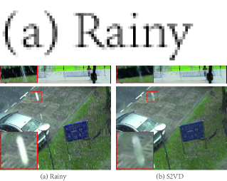
Figure 7: Two typical failure deraining examples by our method. The first row shows a case of large camera motion, while the second row shows another case with heavy rain streaks.

4.2.3 Limitation and Future Direction

Although our method can achieve impressive deraining results as shown above, it may still fails in some real scenarios, e.g., a case with a large camera motion between adjacent time frames and a case with heavy rain streaks. Two failure examples are shown in Fig. 7. The reason is because the adopted MRF prior for unlabeled real data is not strong enough to guarantee satisfactory deraining results in these complicated cases. Therefore, it is urgent and necessary to explore better prior knowledge in order to handle more complicated real deraining tasks in the future.

5 Conclusion

In this paper, we design a dynamical rain generator based on the spatial-temporal process in statistics. With such a dynamical generator, a semi-supervised video deraining method is proposed. Specifically, we represent the sequence of rain layers in rain videos using the dynamical rain generator, which is able to facilitate the rain removal task. To handle the generalization issue for real cases, we propose a semi-supervise learning manner to exploit the common knowledge underlying the synthetic labeled and real unlabeled data sets. Besides, a Monte Carlo-based EM algorithm is designed to learn the model parameters. Extensive experimental results demonstrate the effectiveness of the proposed video deraining method.

Acknowledgement: This research was supported by the National Key R&D Program of China (2020YFA0713900), the China NSFC projects under contracts 11690011, 61721002, U1811461, 62076196.

References

- [1] Peter C Barnum, Srinivasa Narasimhan, and Takeo Kanade. Analysis of rain and snow in frequency space. International Journal of Computer Vision, 86(2-3):256, 2010.
- [2] Jérémie Bossu, Nicolas Hautière, and Jean-Philippe Tarel. Rain or snow detection in image sequences through use of a histogram of orientation of streaks. International Journal of Computer Vision, 93(3):348–367, 2011.
- [3] Nathan Brewer and Nianjun Liu. Using the shape characteristics of rain to identify and remove rain from video. In Joint IAPR International Workshops on Statistical Techniques in Pattern Recognition (SPR) and Structural and Syntactic Pattern Recognition (SSPR), pages 451–458. Springer, 2008.
- [4] Yi Chang, Luxin Yan, and Sheng Zhong. Transformed low-rank model for line pattern noise removal. In Proceedings of the IEEE International Conference on Computer Vision (ICCV), pages 1726–1734, 2017.
- [5] Duan-Yu Chen, Chien-Cheng Chen, and Li-Wei Kang. Visual depth guided color image rain streaks removal using sparse coding. IEEE Transactions on Circuits and Systems for Video Technology, 24(8):1430–1455, 2014.
- [6] Jie Chen, Cheen-Hau Tan, Junhui Hou, Lap-Pui Chau, and He Li. Robust video content alignment and compensation for rain removal in a cnn framework. In Proceedings of the IEEE Conference on Computer Vision and Pattern Recognition (CVPR), pages 6286–6295, 2018.
- [7] Xiaozhi Chen, Kaustav Kundu, Ziyu Zhang, Huimin Ma, Sanja Fidler, and Raquel Urtasun. Monocular 3d object detection for autonomous driving. In Proceedings of the IEEE Conference on Computer Vision and Pattern Recognition (CVPR), pages 2147–2156, 2016.
- [8] Yi-Lei Chen and Chiou-Ting Hsu. A generalized low-rank appearance model for spatio-temporally correlated rain streaks. In Proceedings of the IEEE International Conference on Computer Vision (ICCV), pages 1968–1975, 2013.
- [9] N. Dalal and B. Triggs. Histograms of oriented gradients for human detection. In Proceedings of the IEEE Conference on Computer Vision and Pattern Recognition (CVPR), volume 1, pages 886–893, 2005.
- [10] Arthur P Dempster, Nan M Laird, and Donald B Rubin. Maximum likelihood from incomplete data via the em algorithm. Journal of the Royal Statistical Society: Series B (Methodological), 39(1):1–22, 1977.
- [11] Gianfranco Doretto, Alessandro Chiuso, Ying Nian Wu, and Stefano Soatto. Dynamic textures. International Journal of Computer Vision, 51(2):91–109, 2003.
- [12] Xueyang Fu, Jiabin Huang, Xinghao Ding, Yinghao Liao, and John Paisley. Clearing the skies: A deep network architecture for single-image rain removal. IEEE Transactions on Image Processing, 26(6):2944–2956, 2017.
- [13] Xueyang Fu, Jiabin Huang, Delu Zeng, Yue Huang, Xinghao Ding, and John Paisley. Removing rain from single images via a deep detail network. In Proceedings of the IEEE Conference on Computer Vision and Pattern Recognition (CVPR), pages 3855–3863, 2017.
- [14] Xueyang Fu, Borong Liang, Yue Huang, Xinghao Ding, and John Paisley. Lightweight pyramid networks for image deraining. IEEE Transactions on Neural Networks and Learning Systems, 2019.
- [15] K. Garg and S.K. Nayar. Detection and removal of rain from videos. In Proceedings of the IEEE Conference on Computer Vision and Pattern Recognition (CVPR), volume 1, pages 528–535, 2004.
- [16] Kshitiz Garg and Shree K Nayar. When does a camera see rain? In Proceedings of the IEEE International Conference on Computer Vision (ICCV), volume 2, pages 1067–1074. IEEE, 2005.
- [17] Kshitiz Garg and Shree K Nayar. Photorealistic rendering of rain streaks. ACM Transactions on Graphics (TOG), 25(3):996–1002, 2006.
- [18] Kshitiz Garg and Shree K Nayar. Vision and rain. International Journal of Computer Vision, 75(1):3–27, 2007.
- [19] Shuhang Gu, Deyu Meng, Wangmeng Zuo, and Lei Zhang. Joint convolutional analysis and synthesis sparse representation for single image layer separation. In Proceedings of the IEEE International Conference on Computer Vision (ICCV), pages 1708–1716, 2017.
- [20] Kaiming He, Xiangyu Zhang, Shaoqing Ren, and Jian Sun. Identity mappings in deep residual networks. In Proceedings of the European Conference on Computer Vision (ECCV), pages 630–645, 2016.
- [21] Xiaowei Hu, Chi-Wing Fu, Lei Zhu, and Pheng-Ann Heng. Depth-attentional features for single-image rain removal. In Proceedings of the IEEE Conference on Computer Vision and Pattern Recognition (CVPR), June 2019.
- [22] Kui Jiang, Zhongyuan Wang, Peng Yi, Chen Chen, Baojin Huang, Yimin Luo, Jiayi Ma, and Junjun Jiang. Multi-scale progressive fusion network for single image deraining. In Proceedings of the IEEE Conference on Computer Vision and Pattern Recognition (CVPR), June 2020.
- [23] Tai-Xiang Jiang, Ting-Zhu Huang, Xi-Le Zhao, Liang-Jian Deng, and Yao Wang. A novel tensor-based video rain streaks removal approach via utilizing discriminatively intrinsic priors. In Proceedings of the IEEE Conference on Computer Vision and Pattern Recognition (CVPR), pages 2818–2827, 2017.
- [24] Tai-Xiang Jiang, Ting-Zhu Huang, Xi-Le Zhao, Liang-Jian Deng, and Yao Wang. Fastderain: A novel video rain streak removal method using directional gradient priors. IEEE Transactions on Image Processing, 28(4):2089–2102, 2019.
- [25] Li-Wei Kang, Chia-Wen Lin, and Yu-Hsiang Fu. Automatic single-image-based rain streaks removal via image decomposition. IEEE Transactions on Image Processing, 21(4):1742–1755, 2011.
- [26] Jin-Hwan Kim, Chul Lee, Jae-Young Sim, and Chang-Su Kim. Single-image deraining using an adaptive nonlocal means filter. In Proceedings of the IEEE International Conference on Image Processing (ICIP), pages 914–917, 2013.
- [27] Jin-Hwan Kim, Jae-Young Sim, and Chang-Su Kim. Video deraining and desnowing using temporal correlation and low-rank matrix completion. IEEE Transactions on Image Processing, 24(9):2658–2670, 2015.
- [28] Diederik P. Kingma and Jimmy Lei Ba. Adam: A method for stochastic optimization. In International Conference on Learning Representations (ICLR), 2015.
- [29] Paul Langevin. On the theory of brownian motion. 1983.
- [30] Guanbin Li, Xiang He, Wei Zhang, Huiyou Chang, Le Dong, and Liang Lin. Non-locally enhanced encoder-decoder network for single image de-raining. In Proceedings of the ACM International Conference on Multimedia, pages 1056–1064, 2018.
- [31] Minghan Li, Qi Xie, Qian Zhao, Wei Wei, Shuhang Gu, Jing Tao, and Deyu Meng. Video rain streak removal by multiscale convolutional sparse coding. In Proceedings of the IEEE Conference on Computer Vision and Pattern Recognition (CVPR), pages 6644–6653, 2018.
- [32] Xia Li, Jianlong Wu, Zhouchen Lin, Hong Liu, and Hongbin Zha. Recurrent squeeze-and-excitation context aggregation net for single image deraining. In Proceedings of the European Conference on Computer Vision (ECCV), pages 254–269, 2018.
- [33] Yu Li, Robby T Tan, Xiaojie Guo, Jiangbo Lu, and Michael S Brown. Rain streak removal using layer priors. In Proceedings of the IEEE Conference on Computer Vision and Pattern Recognition (CVPR), pages 2736–2744, 2016.
- [34] Jiaying Liu, Wenhan Yang, Shuai Yang, and Zongming Guo. D3r-net: Dynamic routing residue recurrent network for video rain removal. IEEE Transactions on Image Processing, 28(2):699–712, 2018.
- [35] Jiaying Liu, Wenhan Yang, Shuai Yang, and Zongming Guo. Erase or fill? deep joint recurrent rain removal and reconstruction in videos. In Proceedings of the IEEE Conference on Computer Vision and Pattern Recognition (CVPR), pages 3233–3242, 2018.
- [36] Peng Liu, Jing Xu, Jiafeng Liu, and Xianglong Tang. Pixel based temporal analysis using chromatic property for removing rain from videos. Computer and Information Science, 2(1):53–60, 2009.
- [37] Yu Luo, Yong Xu, and Hui Ji. Removing rain from a single image via discriminative sparse coding. In Proceedings of the IEEE International Conference on Computer Vision (ICCV), pages 3397–3405, 2015.
- [38] Sachin Mehta, Mohammad Rastegari, Anat Caspi, Linda G. Shapiro, and Hannaneh Hajishirzi. Espnet: Efficient spatial pyramid of dilated convolutions for semantic segmentation. In Proceedings of the European Conference on Computer Vision (ECCV), pages 561–580, 2018.
- [39] Pan Mu, Jian Chen, Risheng Liu, Xin Fan, and Zhongxuan Luo. Learning bilevel layer priors for single image rain streaks removal. IEEE Signal Processing Letters, 26(2):307–311, 2018.
- [40] Dongwei Ren, Wangmeng Zuo, Qinghua Hu, Pengfei Zhu, and Deyu Meng. Progressive image deraining networks: A better and simpler baseline. In Proceedings of the IEEE Conference on Computer Vision and Pattern Recognition (CVPR), pages 3937–3946, 2019.
- [41] Weihong Ren, Jiandong Tian, Zhi Han, Antoni Chan, and Yandong Tang. Video desnowing and deraining based on matrix decomposition. In Proceedings of the IEEE Conference on Computer Vision and Pattern Recognition (CVPR), pages 4210–4219, 2017.
- [42] David E Rumelhart, Geoffrey E Hinton, and Ronald J Williams. Learning representations by back-propagating errors. Nature, 323(6088):533–536, 1986.
- [43] Varun Santhaseelan and Vijayan K Asari. Utilizing local phase information to remove rain from video. International Journal of Computer Vision, 112(1):71–89, 2015.
- [44] Andrew M. Saxe, James L. McClelland, and Surya Ganguli. Exact solutions to the nonlinear dynamics of learning in deep linear neural networks. In International Conference on Learning Representations (ICLR), 2014.
- [45] Wenzhe Shi, Jose Caballero, Ferenc Huszár, Johannes Totz, Andrew P Aitken, Rob Bishop, Daniel Rueckert, and Zehan Wang. Real-time single image and video super-resolution using an efficient sub-pixel convolutional neural network. In Proceedings of the IEEE Conference on Computer Vision and Pattern Recognition (CVPR), pages 1874–1883, 2016.
- [46] Chaoyue Wang, Chang Xu, Chaohui Wanga, and Dacheng Tao. Perceptual adversarial networks for image-to-image transformation. IEEE Transactions on Image Processing, pages 4066–4079, 2018.
- [47] Hong Wang, Yichen Wu, Minghan Li, Qian Zhao, and Deyu Meng. A survey on rain removal from video and single image. arXiv preprint arXiv:1909.08326, 2019.
- [48] Hong Wang, Qi Xie, Qian Zhao, and Deyu Meng. A model-driven deep neural network for single image rain removal. In Proceedings of the IEEE Conference on Computer Vision and Pattern Recognition (CVPR), June 2020.
- [49] Hong Wang, Zongsheng Yue, Qi Xie, Qian Zhao, and Deyu Meng. From rain removal to rain generation. arXiv preprint arXiv:2008.03580, 2020.
- [50] Tianyu Wang, Xin Yang, Ke Xu, Shaozhe Chen, Qiang Zhang, and Rynson WH Lau. Spatial attentive single-image deraining with a high quality real rain dataset. In Proceedings of the IEEE Conference on Computer Vision and Pattern Recognition (CVPR), pages 12270–12279, 2019.
- [51] Zhou Wang, Alan C Bovik, Hamid R Sheikh, and Eero P Simoncelli. Image quality assessment: from error visibility to structural similarity. IEEE Transactions on Image Processing, 13(4):600–612, 2004.
- [52] Wei Wei, Deyu Meng, Qian Zhao, Zongben Xu, and Ying Wu. Semi-supervised transfer learning for image rain removal. In Proceedings of the IEEE Conference on Computer Vision and Pattern Recognition (CVPR), pages 3877–3886, 2019.
- [53] Wei Wei, Lixuan Yi, Qi Xie, Qian Zhao, Deyu Meng, and Zongben Xu. Should we encode rain streaks in video as deterministic or stochastic. In Proceedings of the IEEE International Conference on Computer Vision (ICCV), pages 2535–2544, 2017.
- [54] Jianwen Xie, Ruiqi Gao, Zilong Zheng, Song-Chun Zhu, and Ying Nian Wu. Motion-based generator model: Unsupervised disentanglement of appearance, trackable and intrackable motions in dynamic patterns. In The Thirty-Fourth AAAI Conference on Artificial Intelligence, (AAAI), pages 12442–12451, 2020.
- [55] Jianwen Xie, Ruiqi Gao, Zilong Zheng, Song-Chun Zhu, and Ying Nian Wu. Learning dynamic generator model by alternating back-propagation through time. In Proceedings of the AAAI Conference on Artificial Intelligence (AAAI), volume 33, pages 5498–5507, 2019.
- [56] Wenhan Yang, Jiaying Liu, and Jiashi Feng. Frame-consistent recurrent video deraining with dual-level flow. In Proceedings of the IEEE Conference on Computer Vision and Pattern Recognition (CVPR), pages 1661–1670, 2019.
- [57] Wenhan Yang, Robby T Tan, Jiashi Feng, Jiaying Liu, Zongming Guo, and Shuicheng Yan. Deep joint rain detection and removal from a single image. In Proceedings of the IEEE Conference on Computer Vision and Pattern Recognition (CVPR), pages 1357–1366, 2017.
- [58] Wenhan Yang, Robby T Tan, Shiqi Wang, and Jiaying Liu. Self-learning video rain streak removal: When cyclic consistency meets temporal correspondence. In Proceedings of the IEEE Conference on Computer Vision and Pattern Recognition (CVPR), pages 1720–1729, 2020.
- [59] Rajeev Yasarla and Vishal M. Patel. Uncertainty guided multi-scale residual learning-using a cycle spinning cnn for single image de-raining. In Proceedings of the IEEE Conference on Computer Vision and Pattern Recognition (CVPR), June 2019.
- [60] He Zhang and Vishal M Patel. Convolutional sparse and low-rank coding-based rain streak removal. In Proceedings of the IEEE Winter Conference on Applications of Computer Vision (WACV), pages 1259–1267, 2017.
- [61] He Zhang and Vishal M Patel. Density-aware single image de-raining using a multi-stream dense network. In Proceedings of the IEEE Conference on Computer Vision and Pattern Recognition (CVPR), pages 695–704, 2018.
- [62] He Zhang, Vishwanath Sindagi, and Vishal M. Patel. Image de-raining using a conditional generative adversarial network. IEEE Transactions on Circuits and Systems for Video Technology, 2017.
- [63] Kai Zhang, Wangmeng Zuo, and Lei Zhang. Ffdnet: Toward a fast and flexible solution for cnn-based image denoising. IEEE Transactions on Image Processing, 27(9):4608–4622, 2018.
- [64] Xiaopeng Zhang, Hao Li, Yingyi Qi, Wee Kheng Leow, and Teck Khim Ng. Rain removal in video by combining temporal and chromatic properties. In Proceedings of the IEEE International Conference on Multimedia and Expo (ICME), pages 461–464, 2006.
- [65] Yupei Zheng, Xin Yu, Miaomiao Liu, and Shunli Zhang. Residual multiscale based single image deraining. In Proceedings of the British Machine Vision Conference (BMVC), page 147, 2019.
- [66] Lei Zhu, Chi-Wing Fu, Dani Lischinski, and Pheng-Ann Heng. Joint bi-layer optimization for single-image rain streak removal. In Proceedings of the IEEE International Conference on Computer Vision (ICCV), pages 2526–2534, 2017.