Modelling Behavioural Diversity for Learning in Open-Ended Games

Abstract

Promoting behavioural diversity is critical for solving games with non-transitive dynamics where strategic cycles exist, and there is no consistent winner (e.g., Rock-Paper-Scissors). Yet, there is a lack of rigorous treatment for defining diversity and constructing diversity-aware learning dynamics. In this work, we offer a geometric interpretation of behavioural diversity in games and introduce a novel diversity metric based on determinantal point processes (DPP). By incorporating the diversity metric into best-response dynamics, we develop diverse fictitious play and diverse policy-space response oracle for solving normal-form games and open-ended games. We prove the uniqueness of the diverse best response and the convergence of our algorithms on two-player games. Importantly, we show that maximising the DPP-based diversity metric guarantees to enlarge the gamescape – convex polytopes spanned by agents’ mixtures of strategies. To validate our diversity-aware solvers, we test on tens of games that show strong non-transitivity. Results suggest that our methods achieve at least the same, and in most games, lower exploitability than PSRO solvers by finding effective and diverse strategies.

1 Introduction

Nature exhibits a remarkable tendency towards diversity (Holland et al., 1992). Over the past billions of years, natural evolution has discovered a vast assortment of unique species. Each of them is capable of orchestrating, in different ways, the complex biological processes that are necessary to sustain life. Equally, in computer science, machine intelligence can be considered as the ability to adapt to a diverse set of complex environments (Hernández-Orallo, 2017). This suggests that the intelligence of AI evolves with environments of increasing diversity. In fact, recent successes in developing AIs that achieve super-human performance on sophisticated battle games (Vinyals et al., 2019b; Ye et al., 2020) have provided factual justifications for promoting behavioural diversity in training intelligent agents.

In game theory, the necessity of pursuing behavioural diversity is also deeply rooted in the non-transitive structure of games (Balduzzi et al., 2019). In general, an arbitrary game, of either the normal-form type (Candogan et al., 2011) or the differential type (Balduzzi et al., 2018a), can always be decomposed into a sum of two components: a transitive part and a non-transitive part. The transitive part of a game represents the structure in which the rule of winning is transitive (i.e., if strategy A beats B, B beats C, then A beats C), and the non-transitive part refers to the structure in which the set of strategies follows a cyclic rule (e.g., the endless cycles among Rock, Paper and Scissors). Diversity matters especially for the non-transitive part simply because there is no consistent winner in such part of a game: if a player only plays Rock, he can be exploited by Paper, but not so if he has a diverse strategy set of Rock and Scissor.

In fact, many real-world games demonstrate strong non-transitivity (Czarnecki et al., 2020); therefore, it is critical to design objectives in the learning framework that can lead to behavioural diversity. In multi-agent reinforcement learning (MARL) (Yang & Wang, 2020), promoting diversity not only prevents AI agents from checking the same policies repeatedly, but more importantly, helps them discover niche skills, avoid being exploited and maintain robust performance when encountering unfamiliar types of opponents. In the examples of StarCraft (Vinyals et al., 2019b), Soccer (Kurach et al., 2020) and autonomous driving (Zhou et al., 2020), learning a diverse set of strategies has been reported as an imperative step in strengthening AI’s performance.

Despite the importance of diversity (Yang et al., 2021), there is very little work that offers a rigorous treatment in even defining diversity. The majority of work so far has followed a heuristic approach. For example, the idea of co-evolution (Durham, 1991; Paredis, 1995) has drawn forth a series of effective methods, such as open-ended evolution (Standish, 2003; Banzhaf et al., 2016; Lehman & Stanley, 2008), population based training methods (Jaderberg et al., 2019; Liu et al., 2018), and auto-curricula (Leibo et al., 2019; Baker et al., 2019). Despite many empirical successes, the lack of rigorous treatment for behavioural diversity still hinders one from developing a principled approach.

In this work, we introduce a rigorous way of modelling behavioural diversity for learning in games. Our approach offers a new geometric interpretation, which is built upon determinantal point processes (DPP) that have origins in modelling repulsive quantum particles (Macchi, 1977) in physics. A DPP is a special type of point process, which measures the probability of selecting a random subset from a ground set where only diverse subsets are desired. We adapt DPPs to games by formulating the expected cardinality of a DPP as the diversity metric. The proposed diversity metric is a general tool for game solvers; we incorporate our diversity metric into the best-response dynamics, and develop diversity-aware extensions of fictitious play (FP) (Brown, 1951) and policy-space response oracles (PSRO) (Lanctot et al., 2017). Theoretically, we show that maximising the DPP-based diversity metric guarantees an expansion of the gamescape spanned by agents’ mixtures of policies. Meanwhile, we prove the convergence of our diversity-aware learning methods to the respective solution concept of Nash equilibrium and $\alpha$-Rank (Omidshafiei et al., 2019) in two-player games. Empirically, we evaluate our methods on tens of games that show strong non-transitivity, covering both normal-form games and open-ended games. Results confirm the superior performance of our methods, in terms of lower exploitability, against the state-of-the-art game solvers.

2 Related Work

Diversity has been extensively studied in evolutionary computation (EC) (Fogel, 2006) where the central focus is mimicking the natural evolution process. One classic idea in EC is novelty search (Lehman & Stanley, 2011a), which searches for models that lead to different outcomes. Quality-diversity (QD) (Pugh et al., 2016) hybridises novelty search with a fitness objective; two resulting methods are Novelty Search with Local Competition (Lehman & Stanley, 2011b) and MAP-Elites (Mouret & Clune, 2015). For solving games, QD methods were applied to ensure policy diversification among learning agents (Gangwani et al., 2020; Banzhaf et al., 2016). Despite remarkable successes (Jaderberg et al., 2019; Cully et al., 2015), quantifying diversity in EC is often task-dependent and hand-crafted; as a result, building a theoretical understanding of how diversity is generated during learning is non-trivial (Brown et al., 2005).

Searching for behavioural diversity is also a common topic in reinforcement learning (RL). Specifically, it is studied under the names of skill discovery (Eysenbach et al., 2018; Hausman et al., 2018), intrinsic exploration (Gregor et al., 2017; Bellemare et al., 2016; Barto, 2013), or maximum-entropy learning (Haarnoja et al., 2017, 2018; Levine, 2018). These solutions can still be regarded as QD methods, in the sense that the quality refers to the cumulative reward, and dependent on the context, diversity could refer to policies that visit new states (Eysenbach et al., 2018) or have a large entropy (Levine, 2018). Two related works in RL, yet with a different scope, are Q-DPP (Yang et al., 2020b), which adopts DPP to factorise agents’ joint Q-functions in MARL, and DvD (Parker-Holder et al., 2020), which studies diversity based on the ensembles of policy embeddings.

For two-player zero-sum games, smooth FP (Fudenberg & Levine, 1995) is a solver that accounts for diversity through adopting a policy entropy term in the original FP (Brown, 1951). When the game size is large, Double Oracle (DO) (McMahan et al., 2003) provides an iterative method where agents progressively expand their policy pool by, at each iteration, adding one best response versus the opponent’s Nash strategy. Online DO (Dinh et al., 2021) considers a no-regret best response. PSRO generalises FP and DO via adopting a RL subroutine to approximate the best response (Lanctot et al., 2017). Pipeline-PSRO (McAleer et al., 2020) trains multiple best responses in parallel and efficiently solves games of size $10^{50}$. PSRO_rN (Balduzzi et al., 2019) is a specific variation of PSRO that accounts for diversity; however, it suffers from poor performance in a selection of tasks (Muller et al., 2019). Since computing NE is PPAD-Hard (Daskalakis et al., 2009), another important extension of PSRO is $\alpha$-PSRO (Muller et al., 2019), which replaces NE with $\alpha$-Rank (Omidshafiei et al., 2019; Yang et al., 2020a), a solution concept that has polynomial-time solutions on general-sum games. Yet, how to promote diversity in the context of $\alpha$-PSRO is still unknown. In this work, we develop diversity-aware extensions of FP, PSRO and $\alpha$-PSRO, and show on tens of games that our diverse solvers achieve significantly lower exploitability than the non-diverse baselines.

3 Notations & Preliminary

We consider normal-form games (NFGs), denoted by $\langle\mathcal{N},\mathbb{S},{\bm{G}}\rangle$, where each player $i\in\mathcal{N}$ has a finite set of pure strategies $\mathbb{S}^{i}$. Let $\mathbb{S}=\prod_{i\in\mathcal{N}}\mathbb{S}^{i}$ denote the space of joint pure-strategy profiles, and $\mathbb{S}^{-i}$ denote the set of joint strategy profiles except the $i$-th player. A mixed strategy of player $i$ is written by ${\bm{\pi}}^{i}\in\Delta_{\mathbb{S}^{i}}$ where $\Delta$ is a probability simplex. A joint mixed-strategy profile is $\bm{\pi}\in\Delta_{\mathbb{S}}$, and $\bm{\pi}(S)=\prod_{i\in\mathcal{N}}{\bm{\pi}}^{i}(S^{i})$ represents the probability of joint strategy profile $S$. For each $S\in\mathbb{S}$, let ${\bm{G}}(S)=\big{(}{\bm{G}}^{1}(S),...,{\bm{G}}^{N}(S)\big{)}\in\mathbb{R}^{N}$ denote the vector of payoff values for each player. The expected payoff of player $i$ under a joint mixed-strategy profile $\bm{\pi}$ is thus written as ${\bm{G}}^{i}(\bm{\pi})=\sum_{S\in\mathbb{S}}\bm{\pi}(S){\bm{G}}^{i}(S)$, also as ${\bm{G}}^{i}(\bm{\pi}^{i},\bm{\pi}^{-i})$.

3.1 Solution Concepts of Games

Nash equilibrium (NE) exists in all finite games (Nash et al., 1950); it is a joint mixed-strategy profile ${\bm{\pi}}$ in which each player $i\in\mathcal{N}$ plays the best response to other players s.t. ${\bm{\pi}}^{i}\in\mathbf{BR}^{i}({\bm{\pi}}^{-i}):=\arg\max_{{\bm{\pi}}\in\Delta_{S^{i}}}\big{[}{\bm{G}}^{i}({\bm{\pi}},{\bm{\pi}}^{-i})\big{]}$. For $\epsilon>0$, an $\epsilon$-best response to the ${\bm{\pi}}^{-i}$ is $\mathbf{BR}_{\epsilon}^{i}({\bm{\pi}}^{-i}):=\big{\{}{\bm{\pi}}^{i}:{\bm{G}}^{i}\big{(}{\bm{\pi}}^{i},{\bm{\pi}}^{-i}\big{)}\geq{\bm{G}}^{i}\big{(}\mathbf{BR}^{i}({\bm{\pi}}^{-i}),{\bm{\pi}}^{-i}\big{)}-\epsilon\big{\}}$, and an $\epsilon$-NE is a joint profile ${\bm{\pi}}\text{ s.t. }{\bm{\pi}}^{i}\in\mathbf{BR}_{\epsilon}^{i}({\bm{\pi}}),\forall i\in\mathcal{N}$. The exploitability (Davis et al., 2014) measures the distance of a joint strategy profile ${\bm{\pi}}$ to a NE, written as

$$\operatorname{Exploit.}\big{(}{\bm{\pi}}\big{)}=\sum_{i\in\mathcal{N}}\Big{[}{\bm{G}}^{i}\big{(}\mathbf{BR}^{i}({\bm{\pi}}^{-i}),{\bm{\pi}}^{-i}\big{)}-{\bm{G}}^{i}\big{(}{\bm{\pi}}\big{)}\Big{]}.$$ (1)

When the exploitability reaches zero, all players reach their best responses, and thus ${\bm{\pi}}$ is a NE.

Computing NE in multi-player general-sum games is PPAD-Hard (Daskalakis et al., 2009). No polynomial-time solution is available even in two-player cases (Chen et al., 2009). Additionally, NE may not be unique. $\alpha$-Rank (Omidshafiei et al., 2019) is an alternative solution concept, which is built on the response graph of a game. Specifically, $\alpha$-Rank defines the so-called sink strongly-connected components (SSCC) nodes on the response graph that have only incoming edges but no outgoing edges. The SSCC of $\alpha$-Rank serves as a promising replacement for NE; the key associated benefits are its uniqueness, and its polynomial-time solvability in $\mathcal{N}$-player general-sum games. A more detailed description of $\alpha$-Rank can be found in Appendix A.

3.2 Open-Ended Meta-Games

The framework of NFGs is often limited in describing real-world games. In solving games like StarCraft or GO, it is inefficient to list all atomic actions; instead, we are more interested in games at the policy level where a policy can be a “higher-level” strategy (e.g., a RL model powered by a DNN), and the resulting game is a meta-game, denoted by $\langle\mathcal{N},\mathbb{S},{\bm{\mathsfit{M}}}\rangle$. A meta-game payoff table ${\bm{\mathsfit{M}}}$ is constructed by simulating games that cover different policy combinations. With slight abuse of notation, in meta-games, we respectively use $\mathbb{S}^{i}$ to denote the policy set (e.g., a population of deep RL models), and use ${\bm{\pi}}^{i}\in\Delta_{\mathbb{S}^{i}}$ to denote the meta-policy (e.g., player $i$ plays [RL-Model 1, RL-Model 2] with probability [0.3, 0.7]), and thus ${\bm{\pi}}=({\bm{\pi}}^{1},...,{\bm{\pi}}^{N})$ is a joint meta-policy profile. Meta-games are often open-ended because there could exist an infinite number of policies to play a game. The openness also refers to the fact that new strategies will be continuously discovered and added to agents’ policy sets during training; the dimension of ${\bm{\mathsfit{M}}}$ will grow.

In the meta-game analysis (a.k.a. empirical game-theoretic analysis) (Wellman, 2006; Tuyls et al., 2018), traditional solution concepts (e.g., NE or $\alpha$-Rank) can still be computed based on ${\bm{\mathsfit{M}}}$, even in a more scalable manner, this is because the number of “higher-level” strategies in the meta-game is usually far smaller than the number of atomic actions of the underlying game. For example, in tackling StarCraft (Vinyals et al., 2019a), hundreds of deep RL models were trained, which is a trivial amount compared to the number of atomic actions: $10^{26}$ at every time-step.

Many real-world games (e.g., Poker, GO and StarCraft) can be described through an open-ended zero-sum meta-game. Given a game engine $\phi:\mathbb{S}^{1}\times\mathbb{S}^{2}\rightarrow\mathbb{R}$ where $\phi(S^{1},S^{2})>0$ if $S^{1}\in\mathbb{S}^{1}$ beats $S^{2}\in\mathbb{S}^{2}$, and $\phi<0,\phi=0$ refers to losses and ties, the meta-game payoff is

$${\bm{\mathsfit{M}}}=\big{\{}\phi(S^{1},S^{2}):(S^{1},S^{2})\in\mathbb{S}^{1}\times\mathbb{S}^{2}\big{\}}.$$ (2)

A game is symmetric if $\mathbb{S}^{1}\!=\!\mathbb{S}^{2}$ and $\phi(S^{1},S^{2})\!=\!-\phi(S^{2},S^{1}),\forall S^{1},S^{2}\in\mathbb{S}^{1}$; it is transitive if there is a monotonic rating function $f$ such that $\phi(S^{1},S^{2})\!=\!f(S^{1})-f(S^{2}),\forall S^{1},S^{2}\in\mathbb{S}^{1}$, meaning that performance on the game is the difference in ratings; it is non-transitive if $\phi$ satisfies $\sum_{S^{2}\in\mathbb{S}^{2}}\phi(S^{1},S^{2})\!=\!0,\forall S^{1}\in\mathbb{S}^{1}$, meaning that winning against some strategies will be counterbalanced by losses against others; the game has no consistent winner. Lastly, the gamescape of a population of strategies (Balduzzi et al., 2019) in a meta-game is defined as the convex hull of the payoff vectors of all policies in $\mathbb{S}$, written as:

$$\operatorname{Gamescape}\big{(}{\mathbb{S}}\big{)}$$

$$:=\Big{\{}\sum_{i}\alpha_{i}\cdot{\bm{m}}_{i}:\bm{\alpha}\geq 0,\bm{\alpha}^{\top}\mathbf{1}=1,{\bm{m}}_{i}={\bm{\mathsfit{M}}}_{[i,:]}\Big{\}}.$$ (3)

3.3 Game Solvers

In solving NFGs, Fictitious play (FP) (Brown, 1951) describes the learning process where each player chooses a best response to their opponents’ time-average strategies, and the resulting strategies guarantee to converge to the NE in two-player zero-sum, or potential games. Generalised weakened fictitious play (GWFP) (Leslie & Collins, 2006) generalises FP by allowing for approximate best responses and perturbed average strategy updates. It is defined by:

Definition 1 (GWFP)

GWFP is a process of $\{{\bm{\pi}}_{t}\}_{t\geq 0}$ with ${\bm{\pi}}_{t}\in\prod_{i\in\mathcal{N}}\Delta_{\mathbb{S}^{i}},$ following the below updating rule:

$${\bm{\pi}}^{i}_{t+1}\in\big{(}1-\alpha_{t+1}\big{)}{\bm{\pi}}^{i}_{t}+\alpha_{t+1}\big{(}\mathbf{BR}^{i}_{\epsilon_{t}}({\bm{\pi}}_{t}^{-i})+M^{i}_{t+1}\big{)}.$$ (4)

As $t\rightarrow\infty$, $\alpha_{t}\rightarrow 0,\epsilon_{t}\rightarrow 0$ and $\sum_{t\geq 1}\alpha_{n}=\infty$. $\{M_{t}\}_{t\geq 1}$ is a sequence of perturbations that satisfies: $\forall T>0$,

$$\lim_{t\rightarrow\infty}\sup_{k}\bigg{\{}\Big{\|}\sum_{i=t}^{k-1}\alpha_{i+1}M_{i+1}\Big{\|}\text{ s.t. }\sum_{i=n}^{k-1}\alpha_{i}\leq T\bigg{\}}=0.\$$ (5)

GWFP recovers FP if $\alpha_{t}=1/t$, $\epsilon_{t}=0$ and $M_{t}=0,\forall t$.

Table 1: Variations of Different (Meta-)Game Solvers

Method	(Meta-)Policy $\mathcal{S}$	Oracle $\mathcal{O}$	Game type
Self-play (Fudenberg et al., 1998)	$[0,...,0,1]^{N}$	$\mathbf{BR}(\cdot)$	$\mathcal{N}$-player    potential
GWFP (Leslie & Collins, 2006)	$\operatorname{UNIFORM}$	$\mathbf{BR}_{\epsilon}(\cdot)$	2-player zero-sum or potential
D.O. (McMahan et al., 2003)	NE	$\mathbf{BR}(\cdot)$	2-player zero-sum
PSRON (Lanctot et al., 2017)	NE	$\mathbf{BR}_{\epsilon}(\cdot)$	2-player zero-sum
PSROrN (Balduzzi et al., 2019)	NE	Eq. (8)	Symmetric zero-sum
$\alpha$-PSRO (Muller et al., 2019)	$\alpha$-Rank	Eq. (6)	$\mathcal{N}$-player general-sum
Our Methods	NE / $\alpha$-Rank	Eq. (17) / (18)	2-player general-sum

A general solver for open-ended (meta-)games involves an iterative process of solving the equilibrium (meta-)policy first, and then based on the (meta-)policy, finding a new better-performing policy to augment the existing population (see the pseudocode in Appendix B. The (meta-)policy solver, denoted as $\mathcal{S}(\cdot)$, computes a joint (meta-)policy profile ${\bm{\pi}}$ based on the current payoff ${\bm{\mathsfit{M}}}$ (or, ${\bm{G}}$) where different solution concepts can be adopted (e.g., NE or $\alpha$-Rank). With ${\bm{\pi}}$, each agent then finds a new best-response policy, which is equivalent to solving a single-player optimisation problem against opponents’ (meta-)policies ${\bm{\pi}}^{-i}$. One can regard a best-response policy as given by an Oracle, denoted by $\mathcal{O}$. In two-player zero-sum cases, an Oracle represents $\mathcal{O}^{1}({\bm{\pi}}^{2})=\{S^{1}:\sum_{S^{2}\in\mathbb{S}^{2}}{\bm{\pi}}^{2}(S^{2})\cdot\phi(S^{1},S^{2})>0\}$. Generally, Oracles can be implemented through optimisation subroutines such as gradient-descent methods or RL algorithms. After a new policy is learned, the payoff table is expanded, and the missing entries will be filled by running new game simulations. The above process loops over each player at every iteration, and it terminates if no players can find new best-response policies (i.e., Eq. (1) reaches zero).

With correct choices of (meta-)policy solver $\mathcal{S}$ and Oracle $\mathcal{O}$, various types of (meta-)game solvers can be summarised in Table 1. For example, it is trivial to see that GWFP is recovered when $\mathcal{S}=\operatorname{UNIFORM}(\cdot)$ and $\mathcal{O}^{i}=\mathbf{BR}_{\epsilon}^{i}(\cdot)$. Double Oracle (D.O.) and PSRO methods refer to the cases when the (meta-)solver computes NE. Notably, when $\mathcal{S}=\alpha$-Rank, Muller et al. (2019) showed that the standard best response fails to converge to the SSCC of $\alpha$-Rank; instead, they propose $\alpha$-PSRO where the Oracle is computed by the so-called Preference-based Best Response (PBR), that is,

$$\mathcal{O}^{i}\big{(}{\bm{\pi}}^{-i}\big{)}\subseteq\operatorname*{arg\,max}_{\sigma\in\mathbb{S}^{i}}\mathbb{E}_{{\bm{\pi}}^{-i}}\Big{[}\mathds{1}\big{[}{\bm{\mathsfit{M}}}^{i}(\sigma,S^{-i})>{\bm{\mathsfit{M}}}^{i}(S^{i},S^{-i})\big{]}\Big{]}.$$ (6)

3.4 Existing Diversity Measures

Promoting behavioural diversity can lead to learning more effective strategies and achieving lower exploitability in performance. The smooth FP method (Fudenberg & Levine, 1995) incorporates the policy entropy $\mathcal{H}(\pi)$ when finding the best response to advocate diversity, written as $\pi^{i}\in\mathbf{BR}_{\epsilon}^{i}({\bm{\pi}}^{-i})=\arg\max_{\pi\in\Delta_{S^{i}}}\big{[}{\bm{G}}^{i}(\pi,{\bm{\pi}}^{-i})+\tau\cdot\mathcal{H}(\pi)\big{]}$ where $\tau$ is a weighting hyper-parameter. In the case of $\tau\rightarrow 0$ as training goes on, smooth FP converges to the GWFP process almost surely (Leslie & Collins, 2006).

Entropy measures the diversity of a policy in terms of its randomness; however, when it comes to solving open-ended (meta-)games, measuring diversity against peer models in the population becomes critical. Towards this end, effective diversity (ED) (Balduzzi et al., 2019) is proposed to quantify the diversity for a population of policies $\mathbb{S}$ by

$$\operatorname{ED}\big{(}\mathbb{S}\big{)}={{\bm{\pi}}^{*}}^{\top}\left\lfloor{\bm{\mathsfit{M}}}\right\rfloor_{+}{\bm{\pi}}^{*},\ \left\lfloor x\right\rfloor_{+}:=x\text{ if }x\geq 0\text{ else }0.\vspace{-0pt}$$ (7)

${\bm{\mathsfit{M}}}$ is the meta-payoff table of $\mathbb{S}$, and ${\bm{\pi}}^{*}$ is the NE of ${\bm{\mathsfit{M}}}$. The intuition of ED is that, using the Nash distribution ensures that the diversity is only related to the best-responding models, and the rectifier $\left\lfloor x\right\rfloor_{+}$ quantifies the number of variations of how those “winner” models (those within the support of NE) beat each other. Under this design, if there is only one dominant policy in $\mathbb{S}$, then $\operatorname{ED}(\mathbb{S})=0$, thus no diversity. To promote ED in training, a variation of PSRO – PSRO_rN – is introduced, written as:

$$\mathcal{O}^{1}({\bm{\pi}}^{2})=\Big{\{}S^{1}:\sum_{S^{2}\in\mathbb{S}^{2}}{\bm{\pi}}^{2,*}(S^{2})\cdot\lfloor\phi(S^{1},S^{2})\rfloor_{+}>0\Big{\}}.$$ (8)

In short, the ED in PSRO_rN encourages players to amplify its strengths and ignore its weaknesses in finding a new policy. On symmetric zero-sum games, if both players play their Nash strategy (this assumption will be removed by our method), then Eq. (8) guarantees to enlarge the gamescape.

Nonetheless, focusing only on the winners can sometimes be problematic, since weak agents may still hold the promise of tackling niche tasks, and they can serve as stepping stones for discovering stronger policies later during training. For example, when training StarCraft AIs, overcoming agents’ weaknesses was found to be more important than amplifying strengths (Vinyals et al., 2019b), a completely opposite result to PSRO_rN. Another counter example that fails PSRO_rN is the RPS-X game (McAleer et al., 2020):

$${{\bm{G}}=\left[\begin{array}[]{cccc}0&-1&1&-{2}/{5}\\ 1&0&-1&-{2}/{5}\\ -1&1&0&-{2}/{5}\\ {2}/{5}&{2}/{5}&{2}/{5}&0\end{array}\right]}.$$ (13)

In RPS-X, if the initial strategy pool of PSRO_rN starts from either {R}, {P} or {S}, then the algorithm will terminate without exploring the fourth strategy because the best response to {R,P,S} is still in {R,P,S}; however, the fourth strategy alone can still exploit the population of {R,P,S} by getting a positive payoff of $2/5$. Also see in Appendix C how our method can tackle this problem.

4 Our Methods

Instead of choosing between amplifying strengths or overcoming weaknesses, we take an altogether different approach of modelling the behavioural diversity in games. Specifically, we introduce a new diversity measure based on a geometric interpretation of games modelled by a determinantal point process (DPP). Due to the space limit, all proofs in this section are provided in Appendix D.

4.1 Determinantal Point Process

Originating in quantum physics for modelling repulsive Fermion particles (Macchi, 1977; Kulesza et al., 2012), a DPP is a probabilistic framework that characterises how likely a subset of items is to be sampled from a ground set where diverse subsets are preferred. Formally, we have

Definition 2 (DPP)

For a ground set $\mathcal{Y}=\{1,2,...,M\}$, a DPP defines a probability measure $\mathbb{P}$ on the power set of $\mathcal{Y}$ (i.e., $2^{\mathcal{Y}}$), such that, given an $M\times M$ positive semi-definite (PSD) kernel $\bm{\mathcal{L}}$ that measures the pairwise similarity for items in $\mathcal{Y}$, and let $\bm{Y}$ be a random subset drawn from the DPP, the probability of sampling $\forall Y\subseteq\mathcal{Y}$ is written as

$$\operatorname{DPP}(\mathcal{L}):=\mathbb{P}_{\bm{\mathcal{L}}}\big{(}\bm{Y}=Y\big{)}\propto\det\big{(}\bm{\mathcal{L}}_{Y}\big{)}=\operatorname{Volume}^{2}\big{(}\{\bm{w}_{i}\}_{i\in Y}\big{)}$$

where $\bm{\mathcal{L}}_{Y}:=[\bm{\mathcal{L}}_{i,j}]_{i,j\in Y}$ denotes a submatrix of $\bm{\mathcal{L}}$ whose entries are indexed by the items included in $Y$. Given a PSD kernel $\bm{\mathcal{L}}=\bm{\mathcal{W}}\bm{\mathcal{W}}^{\top},\bm{\mathcal{W}}\in\mathbb{R}^{M\times P},P\leq M$, each row $\bm{w}_{i}$ represents a $P$-dimensional feature vector of item $i\in\mathcal{Y}$, then the geometric meaning of $\det(\bm{\mathcal{L}}_{Y})$ is the squared volume of the parallelepiped spanned by the rows of $\bm{\mathcal{W}}$ that correspond to the sampled items in $Y$.

A PSD matrix ensures all principal minors of $\bm{\mathcal{L}}$ are non-negative (i.e., $\det(\bm{\mathcal{L}}_{Y})\geq 0,\forall Y\subseteq\mathcal{Y}$), which suffices to be a proper probability distribution. The normaliser of $\mathbb{P}_{\bm{\mathcal{L}}}(\bm{Y}=Y)$ can be computed by $\sum_{Y\subseteq\mathcal{Y}}\det(\bm{\mathcal{L}}_{Y})=\det(\bm{\mathcal{L}}+\bm{I})$, where $\bm{I}$ is the $M\times M$ identity matrix.

The entries of $\bm{\mathcal{L}}$ are pairwise inner products between item vectors. The kernel $\bm{\mathcal{L}}$ can intuitively be thought of as representing dual effects – the diagonal elements $\bm{\mathcal{L}}_{i,i}$ aim to capture the quality of item $i$, whereas the off-diagonal elements $\bm{\mathcal{L}}_{i,j}$ capture the similarity between the items $i$ and $j$. A DPP models the repulsive connections among the items in a sampled subset. For example, in a two-item subset, since $\small\mathbb{P}_{\bm{\mathcal{L}}}\big{(}\{i,j\}\big{)}\propto\left|\begin{array}[]{ll}{\bm{\mathcal{L}}_{i,i}}&{\bm{\mathcal{L}}_{i,j}}\\ {\bm{\mathcal{L}}_{j,i}}&{\bm{\mathcal{L}}_{j,j}}\end{array}\right|=\bm{\mathcal{L}}_{i,i}\bm{\mathcal{L}}_{j,j}-\bm{\mathcal{L}}_{i,j}\bm{\mathcal{L}}_{j,i}$, we know that if item $i$ and item $j$ are perfectly similar such that $\bm{w}_{i}=\bm{w}_{j}$, and thus $\bm{\mathcal{L}}_{i,j}=\sqrt{\bm{\mathcal{L}}_{i,i}\bm{\mathcal{L}}_{j,j}}$, then these two items will not co-occur, hence such a subset of $Y=\{i,j\}$ will be sampled with probability zero.

4.2 Expected Cardinality: A New Diversity Measure

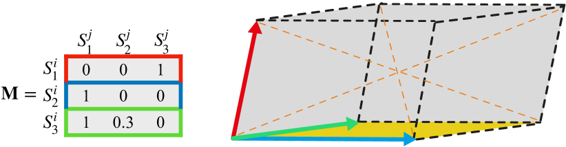
Figure 1: G-DPP. The squared volume of the grey cube equals to $\det(\bm{\mathcal{L}}_{\{S^{i}_{1},S^{i}_{2},S^{i}_{3}\}})$. The probability of selecting $\{S^{i}_{2},S^{i}_{3}\}$ from G-DPP (the yellow area) is smaller than that of selecting $\{S^{i}_{1},S^{i}_{2}\}$ which has orthogonal payoff vectors. The diversity in Eq. (15) of the population $\{S^{i}_{1}\}$,$\{S^{i}_{1},S^{i}_{2}\}$,$\{S^{i}_{1},S^{i}_{2},S^{i}_{3}\}$ are $0,1,1.21$.

Our target is to find a population of diverse policies, with each of them performing differently from other policies due to their unique characteristics. Therefore, when modelling the behavioural diversity in games, we can naturally use the payoff matrix to construct the DPP kernel so that the similarity between two policies depends on their performance in terms of payoffs against different types of opponents.

Definition 3 (G-DPP, Fig. (1))

A G-DPP for each player is a DPP in which the ground set is the strategy population $\mathcal{Y}=\mathbb{S}$, and the DPP kernel $\bm{\mathcal{L}}$ is written by Eq. (14), which is a Gram matrix based on the payoff table ${\bm{\mathsfit{M}}}$.

$$\bm{\mathcal{L}}_{\mathbb{S}}={\bm{\mathsfit{M}}}{\bm{\mathsfit{M}}}^{\top}$$ (14)

For learning in open-ended games, we want to keep adding diverse policies to the population. This is equivalent to say, at each iteration, if we take a random sample from the G-DPP that consists of all existing policies, we hope the cardinality of such a random sample is large (since policies with similar payoff vectors will be unlikely to co-occur!). In this sense, we can design a diversity measure based on the expected cardinality of random samples from a G-DPP, i.e., $\mathbb{E}_{\mathbf{Y}\sim\mathbb{P}_{\mathcal{L}_{\mathbb{S}}}}\big{[}|\mathbf{Y}|\big{]}$. By the following proposition, we show that computing such a diversity measure is tractable.

Proposition 4 (G-DPP Diversity Metric)

The diversity metric, defined as the expected cardinality of a G-DPP, can be computed in $\mathcal{O}(|\mathbb{S}|^{3})$ time by the following equation:

$$\operatorname{Diversity}\big{(}\mathbb{S}\big{)}=\mathbb{E}_{\mathbf{Y}\sim\mathbb{P}_{\mathcal{L}_{\mathbb{S}}}}\big{[}|\mathbf{Y}|\big{]} =\operatorname{Tr}\big{(}\mathbf{I}-(\mathcal{L}_{\mathbb{S}}+\mathbf{I})^{-1}\big{)}.$$ (15)

A nice property of our diversity measure is that it is well-defined even in the case when $\mathcal{Y}$ has duplicated policies, as dealing with redundant policies turns out to be a critical challenge for game evaluation (Balduzzi et al., 2018b). In fact, redundancy also prevents us from directly using $\operatorname{det}\big{(}\mathcal{L_{\mathbb{S}}}\big{)}$ as the diversity measure because the determinant value becomes zero with duplicated entries.

Expected Cardinality vs. Matrix Rank. There is a fundamental difference between using expected cardinality and using the rank of a payoff matrix as the diversity measure. The matrix rank is the maximal number of linearly independent columns, though it can measure the difference between the columns, it cannot model the diversity. For example, in RPS, a strategy of [$99\%$ Rock, $1\%$ Scissor] and a strategy of [$98\%$ Rock, $2\%$ Scissor] are different but they are not diverse as they both favour playing Rock. If one strategy is added into the population whilst the other already exists, the rank of the payoff matrix will increase by one, but the increment on expected cardinality is minor. In Fig. (1), adding the green strategy only contributes to the expected cardinality by $0.21$. This property is particularly important for learning in games, in the sense that finding a diverse policy is often harder than finding just a different policy. To summarise, we show the following proposition.

Proposition 5 (Maximum Diversity)

The diversity of a population $\mathbb{S}$ is bounded by $\operatorname{Diversity}\big{(}\mathbb{S}\big{)}\leq\operatorname{rank}({\bm{\mathsfit{M}}})$, and if ${\bm{\mathsfit{M}}}$ is normalised (i.e., $||{\bm{\mathsfit{M}}}_{[i,:]}||=1,\forall i$), we have $\operatorname{Diversity}\big{(}\mathbb{S}\big{)}\leq\operatorname{rank}({\bm{\mathsfit{M}}})/2$. In both cases, maximal diversity is reached if and only if ${\bm{\mathsfit{M}}}$ is orthogonal.

Expected Cardinality vs. Effective Diversity. We also argue that the principles that underpin Eq. (7) and Eq. (15) are different. Here we illustrate from the perspective of matrix norm. Notably, maximising the effective diversity in Eq. (7) is equivalent to maximising a matrix norm, in the sense that $\operatorname{ED}(\mathbb{S})=\frac{1}{2}\left\|{\bm{\pi}}^{*}\odot{{\bm{\mathsfit{M}}}}\odot{\bm{\pi}}^{*}\right\|_{1,1}$ where $\odot$ is the Hadamard product and $\|\mathbf{A}\|_{1,1}:=\sum_{ij}\left|a_{ij}\right|$. In comparison, the proposition below shows that maximising our diversity measure in Eq. (15) will also maximise the Frobenius norm of ${\bm{\mathsfit{M}}}$.

Proposition 6 (Diversity vs. Matrix Norm)

Maximising the diversity in Eq. (15) also maximises the Frobenius norm of $\|{\bm{\mathsfit{M}}}\|_{F}$, but NOT vice versa.

Geometrically, for a given matrix ${\bm{\mathsfit{M}}}$, considering the box which is the image of a unit cube (in the 3D case) that is stretched by ${\bm{\mathsfit{M}}}$, the Frobenius norm represents the sum of lengths of all diagonals in that box regardless of their directions (the orange lines in Fig. (1)). Therefore, whilst the $\|\cdot\|_{1,1}$ norm reflects the idea that $\operatorname{ED}(\mathbb{S})$ in Eq. (7) accounts for the winners within the Nash support only, the Frobenius norm, on the contrary, considers all strategies’ contribution to diversity. We show later that this results in significant performance improvements over PSRO_rN.

Notably, it is worth highlighting that the opposite direction of Proposition 6 is not correct, that is, maximising $\|{\bm{\mathsfit{M}}}\|_{F}$ will NOT necessarily lead to a large diversity. A counter-example in Fig. (1) is that, if one of the orange lines is long but the rest are short, though the Frobenius norm is large, the expected cardinality is still small. Thus, the diversity metric in Eq. (15) cannot simply be replaced by $\|{\bm{\mathsfit{M}}}\|_{F}$. We also provide empirical evidence in Appendix F.

4.3 Diverse Fictitious Play

With the newly proposed diversity measure of Eq. (15), we can now design diversity-aware learning algorithms. We start by extending the classical FP to a diverse version such that at each iteration, the player not only considers a best response, but also considers how this new strategy can help enrich the existing strategy pool after the update. Formally, our diverse FP method maintains the same update rule as Eq. (4), but with the best response changing into

$$\mathbf{BR}_{\epsilon}^{i}({\bm{\pi}}^{-i})$$

$$=\operatorname*{arg\,max}_{{\bm{\pi}}\in\Delta_{\mathbb{S}^{i}}}\Big{[}{\bm{G}}^{i}\big{(}{\bm{\pi}},{\bm{\pi}}^{-i}\big{)}+\tau\cdot\operatorname{Diversity}\big{(}\mathbb{S}^{i}\cup\{{\bm{\pi}}\}\big{)}\Big{]}$$ (16)

where $\tau$ is a tunable constant. A nice property of diverse FP is that the expected cardinality is guaranteed to be a strictly concave function; therefore, Eq. (16) has a unique solution at each iteration. We have the following proposition:

Proposition 7 (Uniqueness of Diverse Best Response)

Eq. (15) is a strictly concave function. The resulting best response in Eq. (16) has a unique solution.

Intuitively, the diverse FP process will almost surely converge to a GWFP process as long as $\tau\rightarrow 0$ and thus will enjoy the same convergence guarantees as GWFP (i.e., to a NE in two-player zero-sum or potential games). However, in order to prove such connection rigorously, we need to show the sequence of expected changes in strategy, which is induced by finding a strategy that maximises Eq. (16) at each iteration, is actually a uniformly bounded martingale sequence that satisfies Eq. (5). We show the below theorem:

Theorem 8 (Convergence of Diverse FP)

The perturbation sequence induced by diverse FP process is a uniformly bounded martingale difference sequence; therefore, diverse FP shares the same convergence property as GWFP.

4.4 Diverse Policy-Space Oracle

When solving NFGs, the total number of pure strategies is known and thus a best response in Eq. (16) can be computed through a direct search, and the uniqueness of the solution is guaranteed by Proposition 7. When it comes to solving open-ended (meta-)games, the total number of policies is unknown and often infinitely many. Therefore, a best response has to be computed through optimisation subroutines such as gradient-based methods or RL algorithms. Here we extend our diversity measure to the policy space and develop diversity-aware solvers for open-ended (meta-)games.

In solving open-ended games, at the $t$-th iteration, the algorithm maintains a population of policies $\mathbb{S}_{t}^{i}$ learned so far by player $i$. Our goal here is to design an Oracle to train a new strategy $S_{\bm{\theta}}$, parameterised by ${\bm{\theta}}\in\mathbb{R}^{d}$ (e.g., a deep neural net), which both maximises player $i$’s payoff and is diverse from all strategies in $\mathbb{S}_{t}^{i}$. Therefore, we define the ground set of the G-DPP at iteration $t$ to be the union of the existing $\mathbb{S}_{t}^{i}$ and the new model to add: $\mathcal{Y}_{t}=\mathbb{S}_{t}^{i}\cup\big{\{}S_{\bm{\theta}}\big{\}}.$

With the ground set at each iteration, we can compute the diversity measure by Eq. (15). Subsequently, the objective of an Oracle can be written as

$$\mathcal{O}^{1}({\bm{\pi}}^{2})=\operatorname*{arg\,max}_{{\bm{\theta}}\in\mathbb{R}^{d}}\sum_{S^{2}\in\mathbb{S}^{2}} {\bm{\pi}}^{2}\big{(}S^{2}\big{)}\cdot\phi\big{(}S_{\bm{\theta}},S^{2}\big{)}$$ (17)

$$+\tau\cdot\operatorname{Diversity}\Big{(}\mathbb{S}^{1}\cup\big{\{}S_{\bm{\theta}}\big{\}}\Big{)}$$

where ${\bm{\pi}}^{2}(\cdot)$ is the policy of the player two; depending on the game solvers, it can be NE, $\operatorname{UNIFORM}$, etc.

Based on Eq. (17), we can tell that the diversity of policies during training comes from two aspects. The obvious aspect is from the expected cardinality of the G-DPP that forces agents to find diverse policies. The less obvious aspect is from how the opponents are treated. Although the (meta-)policy of player $2$ is determined by ${\bm{\pi}}^{2}(\cdot)$, the learning player will have to focus on exploiting certain aspects of ${\bm{\pi}}^{2}(\cdot)$ in order to acquire diversity. This is similar in manner to selecting a diverse set of opponents. Theoretically, we are able to show that our diversity-aware Oracle can strictly enlarge the gamescape. Unlike PSRO_rN (see Proposition 6 in Balduzzi et al. (2019)), we do NOT need to assume the opponents are playing NE before reaching the result below.

Proposition 9 (Gamescape Enlargement)

Adding a new best-response policy $S_{\bm{\theta}}$ via Eq. (17) strictly enlarges the gamescape. Formally, we have

$$\operatorname{Gamescape}\big{(}{\mathbb{S}}\big{)}\subsetneq\operatorname{Gamescape}\Big{(}{\mathbb{S}\cup\big{\{}S_{\bm{\theta}}\big{\}}}\Big{)}.$$

Implementation of Oracles. When the game engine $\phi$ is differentiable, we can directly apply gradient-based methods to solve Eq. (17). In general, many real-world games are black-box, thus we have to seek for gradient-free solutions or model-free RL algorithms. To tackle this, we provide zero-order Oracle and RL-based Oracle as approximation solutions to Eq. (17), and list their pseudocode and time complexity in Appendix H.

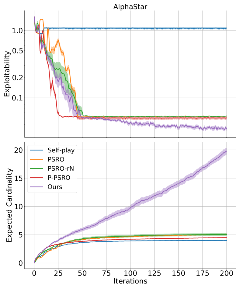
Figure 2: Exploitability and diversity vs. training iterations (number of times a solution concept is computed) on the AlphaStar meta-game (size $888\times 888$). Our method achieves the lowest exploitability by finding a diverse population of $50$ policies.

4.5 Diverse Oracle for $\alpha$-Rank

We also develop diverse Oracles that suit $\alpha$-Rank. Note that $\alpha$-Rank is a replacement solution concept for NE on $\mathcal{N}$-player general-sum games; therefore, the goal of learning is finding all SSCCs on the response graph. Since the standard best response does not have convergence guarantees, we introduce a diversity-aware extension based on $\alpha$-PSRO (Muller et al., 2019) whose Oracle is written in Eq. (6). Specifically, we adopt the quality-diversity decomposition of DPP (Affandi et al., 2014) to unify Eq. (6) and Eq. (15). Given $\bm{\mathcal{L}}=\bm{\mathcal{W}}\bm{\mathcal{W}}^{\top}$, we can rewrite the $i$-th row of $\bm{\mathcal{W}}$ to be the product of a quality term $q_{i}\in\mathbb{R}^{+}$ and a diversity feature $\bm{w}_{i}\in\mathbb{R}^{P}$, thus $\mathcal{L}_{ij}=q_{i}\bm{w}_{i}\bm{w}_{j}^{\top}q_{j}$. We design the quality term to be the exponent of the PBR value in Eq. (6), and the diversity feature follows G-DPP in Eq. (14), that is,

$$q_{i}=\exp\Big{(}\mathbb{E}_{{\bm{\pi}}^{-i}}\big{[}\mathds{1}[{\bm{\mathsfit{M}}}^{i}(\sigma,S^{-i})>{\bm{\mathsfit{M}}}^{i}(S^{i},S^{-i})]\big{]}\Big{)},\bm{w}_{i}=\dfrac{{\bm{\mathsfit{M}}}_{[i,:]}}{\|{\bm{\mathsfit{M}}}\|_{F}}.$$

The resulting diversity-aware Oracle that suits $\alpha$-Rank is:

$$\mathcal{O}_{t}^{i}({\bm{\pi}}^{-i})=\operatorname*{arg\,max}_{{\bm{\pi}}\in\Delta_{\mathbb{S}^{i}}}\operatorname{Tr}\Big{(}\mathbf{I}-\big{(}\bm{\mathcal{L}}_{\mathbb{S}^{i}_{t}\cup\{{\bm{\pi}}\}}+\mathbf{I}\big{)}^{-1}\Big{)}.$$ (18)

The following theorem shows the convergence result of our diverse $\alpha$-PSRO to SSCC on two-player symmetric NFGs.

Theorem 10 (Convergence of Diverse $\alpha$-PSRO)

Diverse $\alpha$-PSRO with the Oracle of Eq. (18) converges to the sub-cycle of the unique SSCC in the two-player symmetric games.

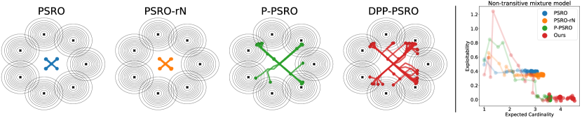
Figure 3: Non-transitive mixture model. Exploration trajectories during training and Performance vs. Diversity comparisons.

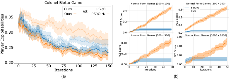
Figure 4: a) Performance of our diverse PSRO vs. PSRO, diverse PSRO vs. PSRO_rN on the Blotto Game, b) PCS-Score comparison of our diverse $\alpha$-PSRO vs. $\alpha$-PSRO on NFGs with variable sizes.

5 Experiments & Results

We compare our diversity-aware solvers with state-of-the-art game solvers including self-play, PSRO (Lanctot et al., 2017), Pipeline-PSRO (McAleer et al., 2020), rectified PSRO (Balduzzi et al., 2019), and $\alpha$-PSRO (Muller et al., 2019). We investigate the performance of these algorithms on both NFGs and open-ended games. Our selected games involve both transitive and non-transitive dynamics. If an algorithm fails to discover a diverse set of policies, it will be trapped in some local strategy cycles that are easily exploitable (e.g., recall the illustrative example of the RPS-X game in Section 3.4, and see how our method can tackle this game in Appendix C. Therefore, we focus on the evaluation metrics of exploitability in Eq. (1) and how extensively the gamescapes are explored. We note that the confidence intervals represented in Figs. (2, 4a, 4b) represent the standard deviation in the exploitability at each iteration over multiple seeds, where the number of seeds is reported in Appendix G. One exception is the comparison between $\alpha$-PSRO and diverse $\alpha$-PSRO, since the solution concept is $\alpha$-Rank, instead of exploitability that measures distance to a NE, we apply the metric of PCS-score (Muller et al., 2019) – the number of SSCC that has been found – for fair comparison. We provide an exhaustive list of hyper-parameter and reward settings in Appendix G.

Real-World Meta-Games. We test our methods on the meta-games that are generated during the process of solving 28 real-world games (Czarnecki et al., 2020), including AlphaStar and AlphaGO. In Fig. (2), we report the results over the AlphaStar game that contained the meta-payoffs for $888$ RL policies, and report the results of the other 27 games in Appendix E. We used Algorithm 2 in Appendix H where agents are defined at the metagame level and correspond to mixed strategies of the underlying game. The results show that our diverse-PSRO method will, at worst, perform as well as existing PSRO baselines, but in many cases (e.g., Fig 2,3,4) will outperform in terms of exploitability, and will always outperform in terms of diversity. In particular, we believe that the performance advantage comes from the fact that without accounting for behavioural diversity, PSRO baselines tend to enter into a cyclic phase where repetitive strategies already in the population are found, whereas our diversifying measure can help discover novel strategies that consequently lead to lower exploitability. While many of the baselines have saturated in finding diverse strategies, our method keeps finding novel effective strategies which leads to a near zero exploitability in almost all $28$ games. In AlphaStar, our method achieves the best performance by only using less than $50$ out of $888$ RL policies, and with the population size growing, the exploitability keeps approaching zero while other methods saturate.

Non-Transitive Mixture Model. This game consists of seven equally-distanced Gaussian humps on the 2D plane. Each strategy corresponds to a point on the 2D plane, which, equivalently, represents the weights that each player puts on the humps, measured by the likelihood of that point in each Gaussian distribution. The payoff of the game that includes both non-transitive and transitive components is given by:

$${\bm{\pi}}^{1,\top}\tiny\left[\begin{array}[]{ccccccc}0&1&1&1&-1&-1&-1\\ -1&0&1&1&1&-1&-1\\ -1&-1&0&1&1&1&-1\\ -1&-1&-1&0&1&1&1\\ 1&-1&-1&-1&0&1&1\\ 1&1&-1&-1&-1&0&1\\ 1&1&1&-1&-1&-1&0\end{array}\right]{\bm{\pi}}^{2}+\frac{1}{2}\sum_{k=1}^{7}({\bm{\pi}}^{1}_{k}-{\bm{\pi}}^{2}_{k}).$$ (26)

Since there are infinite number of points on the 2D plane, this game is open-ended. A winning player must learn to stay close to the Gaussian centroids whilst also exploring all seven Gaussians to avoid being exploited. In Fig. (3), we show the exploration trajectories for different algorithms along with the plot of exploitability vs. diversity. Results suggest that both PSRO and PSRO_rN fail to complete the task; we believe it is due to the same reason as RPS-X where strategy cycling occurs. In contrast, DPP-PSRO solves the task almost perfectly, reaching zero exploitability, by generating a population of diverse and effective strategies.

Colonel Blotto. Blotto is a classical resource allocation game that is widely analysed for election campaigns (Roberson, 2006). In this game, two players have a budget of coins which they simultaneously distribute over a fixed number of areas. An area is won by the player who puts the most coins, and the player that wins the most areas wins the game. We report the results on the game with $3$ areas and $10$ coins over $10$ games. We test how a diverse PSRO player performs in terms of exploitability against a PSRO and a PSRO_rN player, respectively. Fig. (4a) shows that our method (dark colours) consistently achieves a lower exploitability than the opponent player of either PSRO or PSRO_rN (light colours).

Diverse $\alpha$-PSRO. As the PBR in Eq. (6) requires looping through all strategies in $S^{i}$, we test our method on randomly generated zero-sum NFGs with varying dimensions. We do not employ the novelty-bound suggested in Muller et al. (2019) to illustrate how the original $\alpha$-PSRO displays strong cyclic behaviour, which stops it from finding even a few underlying SSCC elements. Results in Fig. (4b) suggest that our diverse $\alpha$-PSRO can effectively prevent the learner from exploring the same strategic cycles during training; it is therefore able to find more SSCCs of $\alpha$-Rank, and outperform $\alpha$-PSRO on the PCS-score.

6 Conclusion

We offer a geometric interpretation of behavioural diversity for learning in games by introducing a new diversity measure built upon the expected cardinality of a DPP. Based on the diversity metric, we propose general solvers for normal-form games and open-ended (meta-)games. We prove the convergence of our methods to NE and $\alpha$-Rank in two-player games, and show theoretical guarantees of expanding the gamescapes. On tens of games, our methods achieve lower exploitability than PSRO variants by finding both effective and diverse strategies.

See pages - of appendix.pdf

References

- Affandi et al. (2014) Affandi, R. H., Fox, E., Adams, R., and Taskar, B. Learning the parameters of determinantal point process kernels. In International Conference on Machine Learning, pp. 1224–1232, 2014.
- Baker et al. (2019) Baker, B., Kanitscheider, I., Markov, T., Wu, Y., Powell, G., McGrew, B., and Mordatch, I. Emergent tool use from multi-agent autocurricula. In International Conference on Learning Representations, 2019.
- Balduzzi et al. (2018a) Balduzzi, D., Racaniere, S., Martens, J., Foerster, J., Tuyls, K., and Graepel, T. The mechanics of n-player differentiable games. In ICML, volume 80, pp. 363–372. JMLR. org, 2018a.
- Balduzzi et al. (2018b) Balduzzi, D., Tuyls, K., Perolat, J., and Graepel, T. Re-evaluating evaluation. In Advances in Neural Information Processing Systems, pp. 3268–3279, 2018b.
- Balduzzi et al. (2019) Balduzzi, D., Garnelo, M., Bachrach, Y., Czarnecki, W., Pérolat, J., Jaderberg, M., and Graepel, T. Open-ended learning in symmetric zero-sum games. In ICML, volume 97, pp. 434–443. PMLR, 2019.
- Banzhaf et al. (2016) Banzhaf, W., Baumgaertner, B., Beslon, G., Doursat, R., Foster, J. A., McMullin, B., De Melo, V. V., Miconi, T., Spector, L., Stepney, S., et al. Defining and simulating open-ended novelty: requirements, guidelines, and challenges. Theory in Biosciences, 135(3):131–161, 2016.
- Barto (2013) Barto, A. G. Intrinsic motivation and reinforcement learning. In Intrinsically motivated learning in natural and artificial systems, pp. 17–47. Springer, 2013.
- Bellemare et al. (2016) Bellemare, M., Srinivasan, S., Ostrovski, G., Schaul, T., Saxton, D., and Munos, R. Unifying count-based exploration and intrinsic motivation. In Advances in neural information processing systems, pp. 1471–1479, 2016.
- Brown et al. (2005) Brown, G., Wyatt, J., Harris, R., and Yao, X. Diversity creation methods: a survey and categorisation. Information Fusion, 6(1):5–20, 2005.
- Brown (1951) Brown, G. W. Iterative solution of games by fictitious play. Activity analysis of production and allocation, 13(1):374–376, 1951.
- Candogan et al. (2011) Candogan, O., Menache, I., Ozdaglar, A., and Parrilo, P. A. Flows and decompositions of games: Harmonic and potential games. Mathematics of Operations Research, 36(3):474–503, 2011.
- Chen et al. (2009) Chen, X., Deng, X., and Teng, S.-H. Settling the complexity of computing two-player nash equilibria. Journal of the ACM (JACM), 56(3):1–57, 2009.
- Cully et al. (2015) Cully, A., Clune, J., Tarapore, D., and Mouret, J.-B. Robots that can adapt like animals. Nature, 521(7553):503–507, 2015.
- Czarnecki et al. (2020) Czarnecki, W. M., Gidel, G., Tracey, B., Tuyls, K., Omidshafiei, S., Balduzzi, D., and Jaderberg, M. Real world games look like spinning tops. arXiv, pp. arXiv–2004, 2020.
- Daskalakis et al. (2009) Daskalakis, C., Goldberg, P. W., and Papadimitriou, C. H. The complexity of computing a nash equilibrium. SIAM Journal on Computing, 39(1):195–259, 2009.
- Davis et al. (2014) Davis, T., Burch, N., and Bowling, M. Using response functions to measure strategy strength. In Proceedings of the AAAI Conference on Artificial Intelligence, volume 28, 2014.
- Dinh et al. (2021) Dinh, L. C., Yang, Y., Tian, Z., Nieves, N. P., Slumbers, O., Mguni, D. H., and Wang, J. Online double oracle. arXiv preprint arXiv:2103.07780, 2021.
- Durham (1991) Durham, W. H. Coevolution: Genes, culture, and human diversity. Stanford University Press, 1991.
- Eysenbach et al. (2018) Eysenbach, B., Gupta, A., Ibarz, J., and Levine, S. Diversity is all you need: Learning skills without a reward function. In International Conference on Learning Representations, 2018.
- Fogel (2006) Fogel, D. B. Evolutionary computation: toward a new philosophy of machine intelligence, volume 1. John Wiley & Sons, 2006.
- Fudenberg & Levine (1995) Fudenberg, D. and Levine, D. Consistency and cautious fictitious play. Journal of Economic Dynamics and Control, 1995.
- Fudenberg et al. (1998) Fudenberg, D., Drew, F., Levine, D. K., and Levine, D. K. The theory of learning in games, volume 2. MIT press, 1998.
- Gangwani et al. (2020) Gangwani, T., Peng, J., and Zhou, Y. Harnessing distribution ratio estimators for learning agents with quality and diversity. arXiv preprint arXiv:2011.02614, 2020.
- Gregor et al. (2017) Gregor, K., Rezende, D. J., and Wierstra, D. Variational intrinsic control. 2017.
- Haarnoja et al. (2017) Haarnoja, T., Tang, H., Abbeel, P., and Levine, S. Reinforcement learning with deep energy-based policies. In ICML, 2017.
- Haarnoja et al. (2018) Haarnoja, T., Zhou, A., Abbeel, P., and Levine, S. Soft actor-critic: Off-policy maximum entropy deep reinforcement learning with a stochastic actor. In International Conference on Machine Learning, pp. 1861–1870, 2018.
- Hausman et al. (2018) Hausman, K., Springenberg, J. T., Wang, Z., Heess, N., and Riedmiller, M. Learning an embedding space for transferable robot skills. In International Conference on Learning Representations, 2018.
- Hernández-Orallo (2017) Hernández-Orallo, J. The measure of all minds: evaluating natural and artificial intelligence. Cambridge University Press, 2017.
- Holland et al. (1992) Holland, J. H. et al. Adaptation in natural and artificial systems: an introductory analysis with applications to biology, control, and artificial intelligence. MIT press, 1992.
- Jaderberg et al. (2019) Jaderberg, M., Czarnecki, W. M., Dunning, I., Marris, L., Lever, G., Castaneda, A. G., Beattie, C., Rabinowitz, N. C., Morcos, A. S., Ruderman, A., et al. Human-level performance in 3d multiplayer games with population-based reinforcement learning. Science, 364(6443):859–865, 2019.
- Kulesza et al. (2012) Kulesza, A., Taskar, B., et al. Determinantal point processes for machine learning. Foundations and Trends® in Machine Learning, 5(2–3):123–286, 2012.
- Kurach et al. (2020) Kurach, K., Raichuk, A., Stańczyk, P., Zajac, M., Bachem, O., Espeholt, L., Riquelme, C., Vincent, D., Michalski, M., Bousquet, O., et al. Google research football: A novel reinforcement learning environment. In Proceedings of the AAAI Conference on Artificial Intelligence, volume 34, pp. 4501–4510, 2020.
- Lanctot et al. (2017) Lanctot, M., Zambaldi, V., Gruslys, A., Lazaridou, A., Tuyls, K., Pérolat, J., Silver, D., and Graepel, T. A unified game-theoretic approach to multiagent reinforcement learning. In Advances in neural information processing systems, pp. 4190–4203, 2017.
- Lehman & Stanley (2008) Lehman, J. and Stanley, K. O. Exploiting open-endedness to solve problems through the search for novelty. In ALIFE, pp. 329–336, 2008.
- Lehman & Stanley (2011a) Lehman, J. and Stanley, K. O. Abandoning objectives: Evolution through the search for novelty alone. Evolutionary computation, 19(2):189–223, 2011a.
- Lehman & Stanley (2011b) Lehman, J. and Stanley, K. O. Evolving a diversity of virtual creatures through novelty search and local competition. In Proceedings of the 13th annual conference on Genetic and evolutionary computation, pp. 211–218, 2011b.
- Leibo et al. (2019) Leibo, J. Z., Hughes, E., Lanctot, M., and Graepel, T. Autocurricula and the emergence of innovation from social interaction: A manifesto for multi-agent intelligence research. arXiv, pp. arXiv–1903, 2019.
- Leslie & Collins (2006) Leslie, D. S. and Collins, E. J. Generalised weakened fictitious play. Games and Economic Behavior, 56(2):285–298, 2006.
- Levine (2018) Levine, S. Reinforcement learning and control as probabilistic inference: Tutorial and review. arXiv preprint arXiv:1805.00909, 2018.
- Liu et al. (2018) Liu, S., Lever, G., Merel, J., Tunyasuvunakool, S., Heess, N., and Graepel, T. Emergent coordination through competition. In International Conference on Learning Representations, 2018.
- Macchi (1977) Macchi, O. The fermion process—a model of stochastic point process with repulsive points. In Transactions of the Seventh Prague Conference on Information Theory, Statistical Decision Functions, Random Processes and of the 1974 European Meeting of Statisticians, pp. 391–398. Springer, 1977.
- McAleer et al. (2020) McAleer, S., Lanier, J., Fox, R., and Baldi, P. Pipeline psro: A scalable approach for finding approximate nash equilibria in large games. arXiv preprint arXiv:2006.08555, 2020.
- McMahan et al. (2003) McMahan, H. B., Gordon, G. J., and Blum, A. Planning in the presence of cost functions controlled by an adversary. In Proceedings of the 20th International Conference on Machine Learning (ICML-03), pp. 536–543, 2003.
- Mouret & Clune (2015) Mouret, J.-B. and Clune, J. Illuminating search spaces by mapping elites. arXiv, pp. arXiv–1504, 2015.
- Muller et al. (2019) Muller, P., Omidshafiei, S., Rowland, M., Tuyls, K., Perolat, J., Liu, S., Hennes, D., Marris, L., Lanctot, M., Hughes, E., et al. A generalized training approach for multiagent learning. In International Conference on Learning Representations, 2019.
- Nash et al. (1950) Nash, J. F. et al. Equilibrium points in n-person games. Proceedings of the national academy of sciences, 36(1):48–49, 1950.
- Omidshafiei et al. (2019) Omidshafiei, S., Papadimitriou, C., Piliouras, G., Tuyls, K., Rowland, M., Lespiau, J.-B., Czarnecki, W. M., Lanctot, M., Perolat, J., and Munos, R. -rank: Multi-agent evaluation by evolution. Scientific reports, 9(1):1–29, 2019.
- Paredis (1995) Paredis, J. Coevolutionary computation. Artificial life, 2(4):355–375, 1995.
- Parker-Holder et al. (2020) Parker-Holder, J., Pacchiano, A., Choromanski, K., and Roberts, S. Effective diversity in population-based reinforcement learning. arXiv preprint arXiv:2002.00632, 2020.
- Pugh et al. (2016) Pugh, J. K., Soros, L. B., and Stanley, K. O. Quality diversity: A new frontier for evolutionary computation. Frontiers in Robotics and AI, 3:40, 2016.
- Roberson (2006) Roberson, B. The colonel blotto game. Economic Theory, 29(1):1–24, 2006.
- Standish (2003) Standish, R. K. Open-ended artificial evolution. International Journal of Computational Intelligence and Applications, 3(02):167–175, 2003.
- Tuyls et al. (2018) Tuyls, K., Perolat, J., Lanctot, M., Leibo, J. Z., and Graepel, T. A generalised method for empirical game theoretic analysis. In Proceedings of the 17th International Conference on Autonomous Agents and MultiAgent Systems, pp. 77–85, 2018.
- Vinyals et al. (2019a) Vinyals, O., Babuschkin, I., Chung, J., Mathieu, M., Jaderberg, M., Czarnecki, W. M., Dudzik, A., Huang, A., Georgiev, P., Powell, R., et al. Alphastar: Mastering the real-time strategy game starcraft ii. DeepMind blog, 2, 2019a.
- Vinyals et al. (2019b) Vinyals, O., Babuschkin, I., Czarnecki, W. M., Mathieu, M., Dudzik, A., Chung, J., Choi, D. H., Powell, R., Ewalds, T., Georgiev, P., et al. Grandmaster level in starcraft ii using multi-agent reinforcement learning. Nature, 575(7782):350–354, 2019b.
- Wellman (2006) Wellman, M. P. Methods for empirical game-theoretic analysis. In AAAI, pp. 1552–1556, 2006.
- Yang & Wang (2020) Yang, Y. and Wang, J. An overview of multi-agent reinforcement learning from game theoretical perspective. arXiv preprint arXiv:2011.00583, 2020.
- Yang et al. (2020a) Yang, Y., Tutunov, R., Sakulwongtana, P., and Ammar, H. B. -rank: Practically scaling -rank through stochastic optimisation. In Proceedings of the 19th International Conference on Autonomous Agents and MultiAgent Systems, pp. 1575–1583, 2020a.
- Yang et al. (2020b) Yang, Y., Wen, Y., Chen, L., Wang, J., Shao, K., Mguni, D., and Zhang, W. Multi-agent determinantal q-learning. ICML, 2020b.
- Yang et al. (2021) Yang, Y., Luo, J., Wen, Y., Slumbers, O., Graves, D., Bou Ammar, H., Wang, J., and Taylor, M. E. Diverse auto-curriculum is critical for successful real-world multiagent learning systems. In Proceedings of the 20th International Conference on Autonomous Agents and MultiAgent Systems, pp. 51–56, 2021.
- Ye et al. (2020) Ye, D., Chen, G., Zhang, W., Chen, S., Yuan, B., Liu, B., Chen, J., Liu, Z., Qiu, F., Yu, H., et al. Towards playing full moba games with deep reinforcement learning. arXiv e-prints, pp. arXiv–2011, 2020.
- Zhou et al. (2020) Zhou, M., Luo, J., Villela, J., Yang, Y., Rusu, D., Miao, J., Zhang, W., Alban, M., Fadakar, I., Chen, Z., et al. Smarts: Scalable multi-agent reinforcement learning training school for autonomous driving. arXiv e-prints, pp. arXiv–2010, 2020.