Simulation Studies on Deep Reinforcement Learning for Building Control with Human Interaction

Abstract

The building sector consumes the largest energy in the world, and there have been considerable research interests in energy consumption and comfort management of buildings. Inspired by recent advances in reinforcement learning (RL), this paper aims at assessing the potential of RL in building climate control problems with occupant interaction. We apply a recent RL approach, called DDPG (deep deterministic policy gradient), for the continuous building control tasks and assess its performance with simulation studies in terms of its ability to handle (a) the partial state observability due to sensor limitations; (b) complex stochastic system with high-dimensional state-spaces, which are jointly continuous and discrete; (c) uncertainties due to ambient weather conditions, occupant’s behavior, and comfort feelings. Especially, the partial observability and uncertainty due to the occupant interaction significantly complicate the control problem. Through simulation studies, the policy learned by DDPG demonstrates reasonable performance and computational tractability.

I Introduction

The building sector is known to consume around 41% of the energy in the United States [3] on an annual basis. For this reason, the building climate control problem has attracted much attention [4, 5, 6] over the past years. Its main goal is to balance between the energy consumption and occupants’ comfort in work environments. In building spaces with occupants, uncertainties are introduced by the action of occupants and incomplete knowledge of their comfort feelings, which are significant in the thermal dynamics of building spaces [7, 8, 9, 10] as well as in deciding the optimal control performance criteria. An important issue that emerged recently is encoding such information into the design process. However, the building system with occupants is a complex stochastic system with high-dimensional jointly continuous and discrete state-spaces, and its real-world control tasks suffer from the partial state observability due to sensor limitations. Therefore, establishing a scalable control design framework is of prime importance. Inspired by recent advances in reinforcement learning (RL) [11, 12], the main goal of this paper is to assess the potential of RL in building climate control problems with occupant interaction.

Optimal control designs for stochastic systems have been a fundamental research field with a long tradition, for instance, the linear quadratic Gaussian problem [13], convex optimization-based design for Markovian disturbances [14], stochastic model predictive control (SMPC) for Gaussian [15] and Markovian [16, 17] disturbance/uncertainties, approximate dynamic programming (ADP) [18, 19] for hybrid electric vehicle powertrain management problems, and scenario-based (or sample-based) approximation approaches for the vehicle path-planning [20, 21], aircraft conflict detection [22], and stochastic MPC [23, 24] to name a few. Most approaches mentioned above formulate the design problems into optimization problems, which however, cannot be easily generalized and scaled to address more generic and complex tasks with high dimensions. On the other hand, reinforcement learning (RL) [25] algorithms provide a sound theoretical/practical framework to address the problem of how an agent learns to take actions to maximize cumulative rewards by interacting with the unknown environment. Recently, significant progress has been made to combine the advances in deep neural network learning [26] with RL [11] to approximate value functions in high-dimensional control- and state-spaces, which has demonstrated successful performance on various challenging control tasks, for example, Atari games [11], AlphaGo [12], and a variety of continuous control problems [27, 28, 29].

For the building control, various stochastic control approaches have been applied. A nonlinear optimization method was studied for SMPC in [30], which was extended in [6] to deal with chance constraints. SMPC was also applied in [31] with weather predictions, and comprehensive guides and surveys were provided in [4]. To cope with generic non-Gaussian stochastic disturbances, a scenario-based SMPC was investigated in [32]. On the other hand, RL has been studied in [33, 34, 35, 36, 37, 38] to find a balance among energy savings, high comfort, and indoor air quality. In particular, experimental and comparative performance analysis of Q-learning was given in [36, 33]. Tabular Q-learning and neural network-based batch Q-learning were implemented in [34, 35]. Other approaches include the fuzzy logic-based Q-learning [37] and Q-learning approach to the lightning and blind control with a user feedback interface [38]. Recently, RL algorithms based on the deep Q-learning [11] was applied to the building problems in [39, 40].

While RL approaches in the building literature are not entirely new, to the authors’ knowledge, the potential of recent advances [27, 28, 29] has not been fully investigated so far. In particular, the majority of RL-based approaches [33, 34, 35, 36, 37, 38, 39, 40] in the building literature employ Q-learning algorithms, which is suitable only with discrete action spaces. For Q-learning algorithms with continuous action spaces, finding the greedy policy requires an optimization of the value function over the continuous action space at every time step [29], which is computationally infeasible in general. However, building spaces conditioned by a VAV (variable air volume) system has continuous action spaces.

Recently, a policy gradient RL for continuous control tasks, called DDPG (deep deterministic policy gradient) algorithm [28, 29], was developed to overcome this challenge based on the actor-critic algorithm [41]. It uses deep neural networks for both actor (deterministic policy) and critic (value function) function approximations and apply a stochastic gradient descent method to maximize the value function and minimize the Bellman loss function. The focus of this paper is to assess the performance of DDGP with simulation studies taking into account occupant-building interactions. We incorporate the occupant comfort feelings into the design and simulation studies. Contrasting with existing approaches, a probabilistic occupant thermal preference model [42, 43] is used directly for training the policy to maintain more comfort indoor air temperature.

Finally, most real-life problems are partially observed, and the building system is no exception. Most SMPC algorithms for the building problems assume that the full state information is available. However, in many building systems, the access to the full system information, such as the ambient weather conditions, is not possible due to limited sensors and building infrastructures. An additional contribution is the consideration of the partial observability in building systems. DDPG algorithm is applied with a direct observation, and its performance is evaluated.

II Problem Formulation

II-A Markov decision process (MDP)

In a Markov decision process with the state-space ${\cal S}:=\{1,2,\ldots,|{\cal S}|\}$ and action-space ${\cal A}:=\{1,2,\ldots,|{\cal A}|\}$, the decision maker selects an action $a\in{\cal A}$ with the current state $s$, then the state transits to $s^{\prime}$ with probability $P(s^{\prime}|s,a)$, and the transition incurs a random reward $r(s,a,s^{\prime})$, $P(s^{\prime}|s,a)$ is the state transition probability from the current state $s\in{\cal S}$ to the next state $s^{\prime}\in{\cal S}$ under action $a\in{\cal A}$, and $r(s,a,s^{\prime})$ is the reward function. The decision maker or agent sequentially takes actions to maximize cumulative discounted rewards. A deterministic policy, $\pi:{\cal S}\to{\cal A}$, maps a state $s\in{\cal S}$ to an action $\pi(s)\in{\cal A}$. The Markov decision problem (MDP) is to find a deterministic or stochastic optimal policy, $\pi^{*}$, such that the cumulative discounted rewards over infinite time horizons is maximized, i.e.,

$$\pi^{*}:=\operatorname{arg\,max}_{\pi\in\Theta}{\mathbb{E}}\left[\left.\sum_{k=0}^{\infty}{\alpha^{k}r(s_{k},a_{k},s_{k+1})}\right|\pi\right],$$

where $\gamma\in[0,1)$ is the discount factor, $\Theta$ is the set of all admissible deterministic policies, $(s_{0},a_{0},s_{1},a_{1},\ldots)$ is a state-action trajectory generated by the Markov chain under policy $\pi$, and ${\mathbb{E}}[\cdot|\cdot,\pi]$ is an expectation conditioned on the policy $\pi$. The Q-function under policy $\pi$ is defined as

$$Q^{\pi}(s,a)= {\mathbb{E}}\left[\left.\sum_{k=0}^{\infty}{\alpha^{k}r(s_{k},a_{k},s_{k+1})}\right|s_{0}=s,a_{0}=a,\pi\right],$$

$$s\in {\cal S},a\in{\cal A},$$

and the corresponding optimal Q-function is defined as $Q^{*}(s,a)=Q^{\pi^{*}}(s,a)$ for all $s\in{\cal S},a\in{\cal A}$. Once $Q^{*}$ is known, then an optimal policy can be retrieved by $\pi^{*}(s)=\operatorname{arg\,max}_{a\in{\cal A}}Q^{*}(s,a)$. When the model is known, the problem can be solved by using the dynamic programming (DP), which tries to solve the Bellman equation [13]. Otherwise, we can use model-free algorithms such as reinforcement learning (RL) [25], which is a class of model-free learning algorithms to find an optimal control of unknown systems by interacting with the unknown environment. For simplicity of the presentation, we only consider MDPs with discrete state and action spaces. However, the arguments in this paper can be generalized to MDPs with continuous state and action spaces or jointly continuous and discrete spaces with some modifications.

II-B Partially Observed MDP (POMDP)

In real world applications, the full-state information is rarely available. The MDP is partially observed when the agent is unable to observe the state $s_{k}$ directly, and instead receives observations from the set ${\cal O}$ which are conditioned on the underlying state $s_{k}$ [27], i.e., there exists a probability distribution $P_{O}(o|s)$ of $o_{k}$ conditioned on the state. The sequential decision problem with this additional constraint is called the partially observable Markov decision problem (POMDP). In a POMDP with the state-space ${\cal S}:=\{1,2,\ldots,|{\cal S}|\}$, action-space ${\cal A}:=\{1,2,\ldots,|{\cal A}|\}$, and observation space ${\cal O}:=\{1,2,\ldots,|{\cal O}|\}$, the decision maker selects an action $a\in{\cal A}$ with the current observation $o\sim P_{O}(\cdot|s)$ conditional on the current state $s$, then the state transits to $s^{\prime}$ with probability $P(s^{\prime}|s,a)$, and the transition incurs a random reward $r(o,a,o^{\prime})$. Usually, the observation $o_{k}$ at time $k$ does not have the Markov property [44, pp. 63], i.e., its transition depends on all the past history of observations and actions. For this reason, an optimal policy may, in principle, require access to the entire history [27] and may in general be non-stationary [45, Fact 4]. In this paper, we restrict our attention to the deterministic stationary policy $\mu:{\cal O}\to{\cal A}$ mapping from $\cal O$ to the control space $\cal A$. To differentiate it from the usual policy based on states, it will be called an output-feedback policy. The decision problem under the output-feedback policy is to find a suboptimal policy, $\mu^{*}$, such that the cumulative discounted rewards over infinite time horizons is maximized, i.e.,

$$\mu^{*}:=\operatorname{arg\,max}_{\pi\in\Pi}{\mathbb{E}}\left[{\left.{\sum_{k=0}^{\infty}{\alpha^{k}r(o_{k},a_{k},o_{k+1})}}\right|\mu}\right],$$

where $\Pi$ is the set of all admissible control policies $\mu:{\cal O}\to{\cal A}$.

In general, RL and DP approaches are applicable only to MDPs with fully observable states because the DP convergence is based on the Markov property, which is lacking in POMDPs. Nevertheless, a naive application of RLs to POMDPs is known to demonstrate reasonable performances in practice [45, 27]. In particular, [45] proved that some RL algorithms solve a modified Bellman equation and compute an approximate policy. The building control problem under our consideration is an POMDP because of the limited access to the full system information, such as the ambient weather conditions. In the next sections, we briefly introduce a naive DDPG algorithm, which will be applied with a direct observation afterwards.

III Deep RL algorithms

RLs can be interpreted as sample-based stochastic dynamic programming (DP) algorithms that solve the Bellman equation. For many important real world problems, the computational requirements of the DP and RL are overwhelming as the state and control spaces are very large. Many RL algorithms [25] use the parameterized Q-factor $Q(\cdot,\cdot|\theta^{Q})$, and approximately solve the Bellman equation with a stream of state observations when the state transition model is not known, as is often the case in real-world applications. In particular, Q-learning [46] solves the Bellman equation with samples/observations by minimizing the loss

$$L(\theta^{Q}):={\mathbb{E}}[(Q(s_{k},a_{k}|\theta^{Q})-y_{k})^{2}],$$

where $y_{k}:=r(s_{k},s_{k},s_{k+1})+\alpha\max_{a\in{\cal A}}Q(s_{k+1},a)|\theta^{Q})$, and the expectation is taken with respect to $s_{k+1},a_{k},s_{k+1}$. Recent RL approaches use large-scale deep neural networks [26], for instance, the deep Q-learning [11] and deep deterministic policy gradient (DDPG) [28, 29], to approximate value functions in high-dimensional spaces. The DDPG is an actor-critic algorithm [41, 47] with neural networks, where a parameterized deterministic control policy (actor), $\pi(s|\theta^{\pi})\in{\cal A},s\in{\cal S}$, instead of the greedy policy and the parameterized Q-factor $Q^{\pi(\cdot|\theta^{\pi})}(s,a)$ (critic) is learned. In particular, it simultaneously performs the two optimizations

$$\theta_{*}^{Q}:= \operatorname{arg\,min}_{\theta^{Q}}L(\theta^{Q})$$

$$:= {\mathbb{E}}_{(s_{k},a_{k},r_{k})\sim U(R)}[(Q(s_{k},a_{k}|\theta^{Q})-y_{k})^{2}],$$

where $y_{k}:=r(s_{k},a_{k},s_{k+1})+\alpha Q(s_{k+1},\pi(s_{k+1}|\theta^{\pi})|\theta^{Q})$, and

$$\theta_{*}^{\pi}:=\operatorname{arg\,max}_{\theta^{\pi}}{\mathbb{E}}_{s_{k}}[Q(s_{k},\pi(s_{k}|\theta^{\pi})|\theta^{Q})].$$

Both the actor and critic parameters are updated by using stochastic gradient descent steps. A naive application of the DDPG to POMDPs is summarized in Algorithm 1.

Algorithm 1 DDPG algorithm [29]

1:Randomly initialize the critic $Q(\cdot,\cdot|\theta^{Q})$ and actor $\mu(\cdot|\theta^{\pi})$ networks with weights $\theta^{Q}$ and $\theta^{\pi}$, respectively.

2:Initialize the so-called target critic network $Q^{\prime}(\cdot,\cdot|\theta^{Q^{\prime}})$ and the target actor network $\mu^{\prime}(\cdot|\theta^{\mu^{\prime}})$ with weights $\theta^{Q^{\prime}}\leftarrow\theta^{Q},\theta^{\mu^{\prime}}\leftarrow\theta^{\mu}$.

3:Initialize the replay buffer ${\cal R}$.

4:for Episodes from $1$ to $M$ do

5:     Initialize a random process ${\cal N}:=(e_{k})_{k=0}^{\infty}$ for action exploration.

6:     Receive the initial state $s_{0}$.

7:     for $k\in\{0,1,\ldots,T-1\}$ do

8:         Select an action $a_{k}=\pi(s_{k}|\theta^{\pi})+e_{k}$ according to the current policy and exploration noise.

9:         Execute the action $a_{k}$, receive the reward $r(s_{k},a_{k},s_{k+1})$ and observe $s_{k+1}$.

10:         Store the transition $(s_{k},a_{k},r(s_{k},a_{k},s_{k+1}),s_{k+1})$ in ${\cal R}$.

11:         Uniformly sample a random minibatch of $N$ transitions $(s_{i},a_{i},r(s_{i},a_{i},s_{i+1}),s_{i+1})$ from ${\cal R}$.

12:         Set $y_{i}=r(s_{i},a_{i},s_{i+1})+\alpha Q^{\prime}(s_{i+1},\pi^{\prime}(s_{i+1}|\theta^{\pi^{\prime}})|\theta^{Q^{\prime}})$.

13:         Update the critic by minimizing the loss $L:=\frac{1}{N}\sum_{i=1}^{N}{(y_{i}-Q(s_{i},a_{i}|\theta^{Q}))^{2}}$.

14:         Update the actor policy using the sampled policy gradient

$$\nabla_{\theta^{\pi}}J^{\pi(\cdot|\theta^{\pi})}$$

$$\cong\frac{1}{N}\sum_{i=1}^{N}{\left.\nabla_{\theta^{\pi}}\pi(s_{i}|\theta^{\pi})\nabla_{a}Q(s_{i},a|\theta^{Q})\right|_{a=\pi(s_{i}|\theta^{\pi})}}.$$

15:         Update the target networks

$$\theta^{Q^{\prime}}\leftarrow\tau\theta^{Q}+(1-\tau)\theta^{Q^{\prime}},\quad\theta^{\pi^{\prime}}\leftarrow\tau\theta^{\pi}+(1-\tau)\theta^{\pi^{\prime}},$$

where $\tau\in(0,1)$ is the update step size.

16:     end for

17:end for

The algorithm can be applied to POMDPs with $(o_{k},o_{k+1},\pi)$ replaced with $(s_{k},s_{k+1},\mu)$.

IV Building Control with Occupant Interaction

IV-A Building Model

We consider a $3{\rm m}\times 3{\rm m}$ private office space with a $2.5{\rm m}^{2}$ south facing window, and its RC (resistor-capacitor) circuit analogy is given in Figure 1. To reduce the order of the model, we use one node for air in the room and another node collecting all the thermal mass in the room,

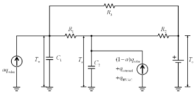
Figure 1: RC circuit analogy

where ${\bf T}_{\rm a}$ is the air temperature (${}^{\circ}C$), ${\bf T}_{\rm o}$ is the outdoor air temperature (${}^{\circ}C$), ${\bf T}_{\rm w}$ is the temperature of the aggregated mass node (${}^{\circ}C$), ${\bf q}_{\rm solar}$ is the solar radiation ($W$), ${\bf q}_{\rm internal}$ is the internal heat ($W$), ${\bf q}_{\rm HVAC}$ is the heating/cooling rate of the HVAC (heating, ventilating, and air-conditioning) system ($W$). We assume that the room is conditioned by a VAV (variable air volume) system so that ${\bf q}_{\rm HVAC}$ directly affects ${\bf T}_{\rm a}$. Since we use low order model, we assume that the air node includes some portion of surfaces in the room which absorb radiative heat and release the heat quickly to the air. To determine appropriate values of the parameters of the circuit, we conducted a building energy simulation with EnergyPlus 8.7.0 in [48], and estimated the parameters minimizing the root-mean-square error between the air temperatures calculated by the EnergyPlus simulation and the low order model. The values of parameters are summarized in Table I. Moreover, all notations used to describe the building system are presented in Table II.

TABLE I: Values of the parameters of the circuit in Figure 1

Parameter	Value	Unit
$R_{1}$	$0.0084197$	${}^{\circ}C/W$
$R_{2}$	$0.044014$	${}^{\circ}C/W$
$R_{3}$	$4.38$	${}^{\circ}C/W$
$C_{1}$	$9861100$	$J/^{\circ}C$
$C_{2}$	$128560$	$J/^{\circ}C$
$a$	$0.55$	–

TABLE II: Notations

Notation	Meaning
${\bf T}_{\rm a}$	Indoor air temperature (${}^{\circ}C$)
${\bf T}_{\rm o}$	Outdoor air temperature (${}^{\circ}C$)
${\bf T}_{\rm w}$	Temperature of the aggregated mass node (${}^{\circ}C$)
${\bf q}_{\rm solar}$	Solar radiation ($W$)
${\bf q}_{\rm internal}$	Internal heat ($W$)
${\bf q}_{\rm HVAC}$	Heating/cooling rate of the HVAC system ($W$)
$\Delta t$	Sampling time (min)

The dynamic system model is given as

$$C_{2}\dot{\bf T}_{{\rm a},t}=\frac{{\bf T}_{{\rm o},t}-{\bf T}_{{\rm a},t}}{R_{2}}+\frac{{\bf T}_{{\rm w},t}-{\bf T}_{{\rm a},t}}{R_{1}}$$

$$+(1-a){\bf q}_{{\rm solar},t}+{\bf q}_{{\rm HVAC},t}+{\bf q}_{{\rm internal},t},$$

$$C_{1}\dot{\bf T}_{{\rm w},t}=\frac{{\bf T}_{a,t}-{\bf T}_{w,t}}{R_{1}}+\frac{{\bf T}_{{\rm o},t}-{\bf T}_{{\rm w},t}}{R_{3}}+a{\bf q}_{{\rm solar},t}.$$

A discrete time representation can be obtained by using the Euler discretization with a sampling time of $\Delta t$

$${\bf T}_{{\rm a},k+1}-{\bf T}_{{\rm a},k}=\frac{\Delta t}{C_{2}R_{2}}({\bf T}_{{\rm o},k}-{\bf T}_{{\rm a},k})$$

$$+\frac{\Delta t}{C_{2}R_{1}}({\bf T}_{{\rm w},k}-{\bf T}_{{\rm a},k})+\frac{\Delta t(1-a)}{C_{2}}{\bf q}_{{\rm solar},k}$$

$$+\frac{\Delta t}{C_{2}}{\bf q}_{{\rm HVAC},k}+\frac{\Delta t}{C_{2}}{\bf q}_{{\rm internal},k},$$

$${\bf T}_{{\rm w},k+1}-{\bf T}_{{\rm w},k}=\frac{\Delta t}{C_{1}R_{1}}({\bf T}_{{\rm a},k}-{\bf T}_{{\rm w},k})$$

$$+\frac{\Delta t}{C_{1}R_{3}}({\bf T}_{{\rm o},k}-{\bf T}_{{\rm w},k})+\frac{\Delta ta}{C_{1}}{\bf q}_{{\rm solar},k},$$ (1)

where $k\geq 0$ is the discrete time step. Here, we consider $\Delta t=10{\rm min}$ sampling time, which is a finer time-scale than the time step $\Delta t=30{\rm min}$ which is usually used in the building research literature in order to consider changes of occupant’s thermal comfort.

IV-B Occupant and Weather Models

A stochastic process $({\bf z}_{k})_{k=0}^{\infty}$ with the state-space $\{1,2,3\}$ represents the occupant’s feelings of cold, comfort, and hot, respectively. Its probability mass function $p(i;{\bf T}_{\rm a})$, $i\in\{1,2,3\}$, depending on the air temperature, ${\bf T}_{\rm a}$, is obtained by the Bayesian modelling approach [42] and is depicted in Figure 2 for different ${\bf T}_{\rm a}$.

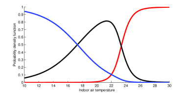
Figure 2: The probability density function $p(1;{\bf T}_{\rm a})$ (blue), $p(2;{\bf T}_{\rm a})$ (black), $p(3;{\bf T}_{\rm a})$ (red) for different $T_{\rm a}$

We consider the stochastic function ${\bf M}_{k}:\{0,1,\ldots,143\}\to\{0,1\}$ to represent the occupancy at time step $k\in\{0,1,\ldots,143\}$. The occupant arrives at the room at time ${\bf w}_{1}$ which is a random variable uniformly distributed within $\{48,\ldots,54\}$ (between 8am and 9am) and leaves the room at time ${\bf w}_{2}$ which is a random variable uniformly distributed within $\{96,\ldots,114\}$ (between 4pm and 7pm). ${\bf M}_{k}=1$ if the room is occupied at time $k$ and ${\bf M}_{k}=0$ otherwise.

The 24 hours real weather histories $({\bf T}_{{\rm o},k},{\bf q}_{{\rm solar},k})_{k=0}^{143}$ over 31 days are collected during July, 2017, in West Lafayette, Indiana, USA, and are used to approximate them into a Markov chain. In particular, the outdoor temperature within the range $[10,40]$ is discretized into 6 points, $12.5$, $17.5$,$22.5$, $27.5$, $32.5$, and $37.5$ and augmented with the periodic time step $k\in\{0,1,\ldots,143\}$, which is periodically initialized to $k=0$ after the last time step $k=143$, to form $6\times 144$ the state-space. We constructed a Markov chain with this state space. Similarly, the solar radiation within the range $[0,900]$ is discretized into 9 points, $50$, $150,\ldots,850$ and augmented with time $k$ to form a state-space with size $9\times 144$. A Markov chain with this state-space was constructed in a similar way.

IV-C Overall State-Space Model

From the discretized model (1), we obtain a state-space model ${\bf x}_{k+1}=A{\bf x}_{k}+B{\bf u}_{k}+D{\bf x}_{k}$ with ${\bf u}_{k}={\bf q}_{{\rm HVAC},k}$,

$${\bf x}_{k}=\begin{bmatrix}{\bf T}_{{\rm a},k}\\ {\bf T}_{{\rm w},k}\\ \end{bmatrix},\,{\bf w}_{k}=\begin{bmatrix}{\bf q}_{{\rm solar},k}\\ {\bf q}_{{\rm internal},k}\\ {\bf T}_{{\rm o},k}\\ \end{bmatrix},$$ (2)

and

$$A=\begin{bmatrix}1-\frac{\Delta t}{C_{2}R_{2}}-\frac{\Delta t}{C_{2}R_{1}}&\frac{\Delta t}{C_{2}R_{1}}\\ \frac{\Delta t}{C_{1}R_{1}}&1-\frac{\Delta t}{C_{1}R_{3}}-\frac{\Delta t}{C_{1}R_{1}}\\ \end{bmatrix},$$

$$B=\begin{bmatrix}\frac{\Delta t}{C_{2}}\\ 0\\ \end{bmatrix},\quad D=\begin{bmatrix}\frac{\Delta t(1-a)}{C_{2}}&\frac{\Delta t}{C_{2}}&\frac{\Delta t}{C_{2}R_{2}}\\ \frac{\Delta ta}{C_{1}}&0&\frac{\Delta t}{C_{1}R_{3}}\\ \end{bmatrix}.$$

The internal heat is ${\bf q}_{{\rm internal},k}=75+70{\bf M}_{k}$ ($W$), where the first term, $75$, is internal heat due to electronic appliances, and the second term, $70{\bf M}_{k}$, indicates the heat produced by the occupant. The complete discrete state including the weather conditions is

$${\bf s}_{k}=\begin{bmatrix}{\bf x}_{k}^{T}&{\bf z}_{k}&(k\,{\rm mod}\,144)&{\bf T}_{{\rm o},k}&{\bf q}_{{\rm solar},k}&{\bf M}_{k}\\ \end{bmatrix}^{T},$$

where $(k\,{\rm mod}\,144)$ is the remainder of $k$ divided by $144$ and represents the 24 hours periodic time steps. We assume that the occupant’s comfort level ${\bf z}_{k}$, wall temperature ${\bf T}_{{\rm w},k}$, outdoor temperature ${\bf T}_{{\rm o},k}$, and solar radiation ${\bf T}_{{\rm solar},k}$ cannot be observed. Therefore, the observation is

$${\bf o}_{k}=\begin{bmatrix}{\bf T}_{{\rm a},k}&(k\,{\rm mod}\,144)&{\bf M}_{k}\\ \end{bmatrix}^{T}.$$ (3)

IV-D Reward Design

In general, the reward function for RL-based designs is hand-engineered with trial and errors to demonstrate reasonable control performances. Since the performance of the learned policy depends considerably on the reward, there exist approaches to design rewards, for instance, the inverse RL [49]. However, these approaches will not be considered here. We first introduce a hand-crafted cost function ${\bf c}({\bf s}_{k},{\bf u}_{k})$, and then set ${\bf r}({\bf s}_{k},{\bf u}_{k})=-{\bf c}({\bf s}_{k},{\bf u}_{k})$ to minimize the long term discounted costs. In particular, the cost function is set to be

$${\bf c}({\bf s}_{k},{\bf u}_{k}):=\begin{cases}0.001{\bf u}_{k}^{2}\quad{\rm if}\,\,\,{\bf M}_{k}=0\\ 0.00001{\bf u}_{k}^{2}+{\bf c}_{1,k}+{\bf c}_{2,k}\quad{\rm if}\,\,\,{\bf M}_{k}=1\\ \end{cases}$$

where ${\bf c}_{1,k}$ is the penalty term related to the state constraint ${\bf T}_{a,k}\in[20,30]$:

$${\bf c}_{1,k}=\begin{cases}0\quad{\rm if}\,\,{\bf T}_{a,k}\,\in[20,30]\\ 200\quad{\rm otherwise}\\ \end{cases}$$

and ${\bf c}_{3,k}$ is the penalty term related to the comfort of the occupant:

$${\bf c}_{2,k}=\begin{cases}0\quad{\rm if}\,\,{\bf z}_{k}=2\\ 100\quad{\rm if}\,\,{\bf z}_{k}\in\{1,3\}\\ \end{cases}$$

IV-E Simulation

For simulation studies, we implement the DDPG using Python. This work uses neural networks with four hidden layers of width $(1024,1024,512,512)$ for both actor and critic networks. We implemented Algorithm 1 with approximately two hours of training. Simulation results of a one week operation under the learned policy are given in Figure 3. The fifth day’s results in Figure 3 are plotted in Figure 4, which shows that without observations of the outdoor temperature and solar radiation, the trained policy infers the decrease of the the outdoor temperature/solar radiation, and starts to decrease the input power. For a comparative analysis, a greedy policy is considered, which minimizes a cost function based on the one-step-ahead prediction of the system trajectory. In particular, the greedy policy ${\bf u}_{k}=\mu({\bf x}_{k},{\bf w}_{k},{\bf M}_{k})$ is defined as

$$\mu({\bf x}_{k},{\bf w}_{k},{\bf M}_{k}):=\begin{cases}{\bf u}_{k}^{*}\quad{\rm if}\,\,{\bf M}_{k}=1\\ 0\quad{\rm otherwise}\\ \end{cases}$$ (4)

where

$${\bf u}_{k}^{*}:=\operatorname{arg\,min}_{|u|\leq 1000}\{\gamma([{\bf x}_{k+1}]_{1}-22)^{2}+10^{-5}u^{2}\},$$

$[{\bf x}_{k+1}]_{1}$ is the first element of ${\bf x}_{k+1}$, ${\bf x}_{k+1}=A{\bf x}_{k}+B{\bf u}_{k}+D{\bf w}_{k}$, and the number 22 is the temperature that maximizes the comfort probability, i.e., $22\cong\operatorname{arg\,max}_{T_{a}}p(2;T_{a})$. The policy tries to enforce the current indoor air temperature to be 22$C^{\circ}$ while minimizing the current control input energy. One week simulation results under the greedy control policy are given in Figure 5. The fifth day’s results are plotted in Figure 6.

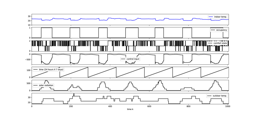
Figure 3: One week simulation results with a policy learned by DDPG. The indoor air temperature (blue solid line), occupancy, control input, time steps which reset every 24 hours, solar radiation, and outdoor air temperature from the top to bottom figures.

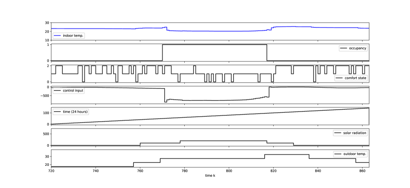
Figure 4: The fifth day results of Figure 3.

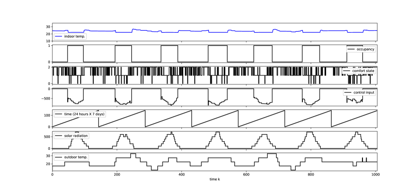
Figure 5: One week simulation results with the greedy policy (4). The indoor air temperature (blue solid line), occupancy, control input, time steps which reset every 24 hours, solar radiation, and outdoor air temperature from the top to bottom figures.

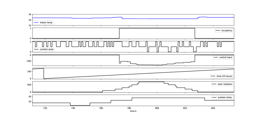
Figure 6: The fifth day results of Figure 5.

Histograms of the total input energy (kJ) during a single day are depicted in Figure 7 for the RL policy (top figure) and the greedy policy (bottom figure) with 5000 samples.

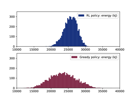
Figure 7: Histograms of the total input energy (kJ) during a single day for the RL policy (top figure) and the greedy policy (bottom figure).

In addition, histograms of the total comfort scores during a single day are illustrated in Figure 8 for the RL policy (top figure) and the greedy policy (bottom figure). During a single day, the comfort score is computed by counting the total number of comfort feelings, i.e., ${\bf z}_{k}=2$, when the room is occupied. From the results, one concludes that both policies demonstrate similar performances. However, the policy learned by DDPG only uses a direct observation (3), while the greedy policy (4) requires the full knowledge of the system state at every time steps.

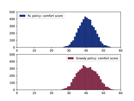
Figure 8: Histograms of the total comfort scores during a single day for the RL policy (top figure) and the greedy policy (bottom figure).

Conclusion

The building climate control problem with occupant interactions is an active topic. This paper has presented an application of DDPG approach to the building problem and assessed its performance. Comparative simulation results have suggested that the policy learned by DDPG outperforms other methods. The results were based on the simulation-based off-line learning, which is possible only when an overall model of the building system is known. Future research will focus on a real-world implementation of the RL with occupant interactions. In this case, the real-time RL requires a real-time user feedback interface with a voting system to learn the policy based on the occupant’s satisfaction.

References

- [1] D. Lee, S. Lee, P. Karava, and J. Hu, “Simulation-based policy gradient and its building control application,” in Proc. American control conference (ACC2018), Milwaukee, USA, 2018.
- [2] ——, “Approximate dynamic programming for building control problems with occupant interactions,” in Proc. American control conference (ACC2018), Milwaukee, USA, 2018.
- [3] 2011 Buildings Energy Data Book, U.S. Dept. Energy, Washington, DC, USA, 2011.
- [4] Y. Ma, A. Kelman, A. Daly, and F. Borrelli, “Predictive control for energy efficient buildings with thermal storage,” IEEE Control system magazine, vol. 32, no. 1, pp. 44–64, 2012.
- [5] A. I. Dounis and C. Caraiscos, “Advanced control systems engineering for energy and comfort management in a building environment–A review,” Renewable and Sustainable Energy Reviews, vol. 13, no. 6, pp. 1246–1261, 2009.
- [6] Y. Ma, S. Vichik, and F. Borrelli, “Fast stochastic MPC with optimal risk allocation applied to building control systems,” in 2012 IEEE 51st IEEE Conference on Decision and Control (CDC), 2012, pp. 7559–7564.
- [7] A. Aswani, N. Master, J. Taneja, D. Culler, and C. Tomlin, “Reducing transient and steady state electricity consumption in hvac using learning-based model-predictive control,” Proceedings of the IEEE, vol. 100, no. 1, pp. 240–253, 2012.
- [8] F. Oldewurtel, D. Sturzenegger, and M. Morari, “Importance of occupancy information for building climate control,” Applied energy, vol. 101, pp. 521–532, 2013.
- [9] J. R. Dobbs and B. M. Hencey, “Model predictive hvac control with online occupancy model,” Energy and Buildings, vol. 82, pp. 675–684, 2014.
- [10] J. Page, D. Robinson, N. Morel, and J.-L. Scartezzini, “A generalised stochastic model for the simulation of occupant presence,” Energy and buildings, vol. 40, no. 2, pp. 83–98, 2008.
- [11] V. Mnih, K. Kavukcuoglu, D. Silver, A. A. Rusu, J. Veness, M. G. Bellemare, A. Graves, M. Riedmiller, A. K. Fidjeland, G. Ostrovski et al., “Human-level control through deep reinforcement learning,” Nature, vol. 518, no. 7540, pp. 529–533, 2015.
- [12] D. Silver, A. Huang, C. J. Maddison, A. Guez, L. Sifre, G. Van Den Driessche, J. Schrittwieser, I. Antonoglou, V. Panneershelvam, M. Lanctot et al., “Mastering the game of go with deep neural networks and tree search,” nature, vol. 529, no. 7587, pp. 484–489, 2016.
- [13] D. P. Bertsekas and J. N. Tsitsiklis, Neuro-dynamic programming. Athena Scientific Belmont, MA, 1996.
- [14] O. L. V. Costa, E. Assumpção Filho, E. K. Boukas, and R. Marques, “Constrained quadratic state feedback control of discrete-time markovian jump linear systems,” Automatica, vol. 35, no. 4, pp. 617–626, 1999.
- [15] J. A. Primbs and C. H. Sung, “Stochastic receding horizon control of constrained linear systems with state and control multiplicative noise,” IEEE Transactions on Automatic Control, vol. 54, no. 2, pp. 221–230, 2009.
- [16] P. Patrinos, P. Sopasakis, H. Sarimveis, and A. Bemporad, “Stochastic model predictive control for constrained discrete-time markovian switching systems,” Automatica, vol. 50, no. 10, pp. 2504–2514, 2014.
- [17] S. Di Cairano, D. Bernardini, A. Bemporad, and I. V. Kolmanovsky, “Stochastic mpc with learning for driver-predictive vehicle control and its application to hev energy management,” IEEE Transactions on Control Systems Technology, vol. 22, no. 3, pp. 1018–1031, 2014.
- [18] I. V. Kolmanovsky, L. Lezhnev, and T. L. Maizenberg, “Discrete-time drift counteraction stochastic optimal control: Theory and application-motivated examples,” Automatica, vol. 44, no. 1, pp. 177–184, 2008.
- [19] L. Johannesson, M. Asbogard, and B. Egardt, “Assessing the potential of predictive control for hybrid vehicle powertrains using stochastic dynamic programming,” IEEE Transactions on Intelligent Transportation Systems, vol. 8, no. 1, pp. 71–83, 2007.
- [20] L. Blackmore, A. Bektassov, M. Ono, and B. C. Williams, “Robust, optimal predictive control of jump markov linear systems using particles,” in International Workshop on Hybrid Systems: Computation and Control, 2007, pp. 104–117.
- [21] L. Blackmore, M. Ono, A. Bektassov, and B. C. Williams, “A probabilistic particle-control approximation of chance-constrained stochastic predictive control,” IEEE Transactions on Robotics, vol. 26, no. 3, pp. 502–517, 2010.
- [22] M. Prandini, J. Hu, J. Lygeros, and S. Sastry, “A probabilistic approach to aircraft conflict detection,” IEEE Transactions on intelligent transportation systems, vol. 1, no. 4, pp. 199–220, 2000.
- [23] G. Schildbach, L. Fagiano, C. Frei, and M. Morari, “The scenario approach for stochastic model predictive control with bounds on closed-loop constraint violations,” Automatica, vol. 50, no. 12, pp. 3009–3018, 2014.
- [24] G. C. Calafiore and L. Fagiano, “Robust model predictive control via scenario optimization,” IEEE Transactions on Automatic Control, vol. 58, no. 1, pp. 219–224, 2013.
- [25] R. S. Sutton and A. G. Barto, Reinforcement learning: An introduction. MIT Press, 1998.
- [26] Y. LeCun, Y. Bengio, and G. Hinton, “Deep learning,” Nature, vol. 521, no. 7553, pp. 436–444, 2015.
- [27] N. Heess, J. J. Hunt, T. P. Lillicrap, and D. Silver, “Memory-based control with recurrent neural networks,” arXiv preprint arXiv:1512.04455, 2015.
- [28] D. Silver, G. Lever, N. Heess, T. Degris, D. Wierstra, and M. Riedmiller, “Deterministic policy gradient algorithms,” in ICML, 2014.
- [29] T. P. Lillicrap, J. J. Hunt, A. Pritzel, N. Heess, T. Erez, Y. Tassa, D. Silver, and D. Wierstra, “Continuous control with deep reinforcement learning,” arXiv preprint arXiv:1509.02971, 2015.
- [30] Y. Ma and F. Borrelli, “Fast stochastic predictive control for building temperature regulation,” in American Control Conference (ACC), 2012, 2012, pp. 3075–3080.
- [31] F. Oldewurtel, A. Parisio, C. N. Jones, D. Gyalistras, M. Gwerder, V. Stauch, B. Lehmann, and M. Morari, “Use of model predictive control and weather forecasts for energy efficient building climate control,” Energy and Buildings, vol. 45, pp. 15–27, 2012.
- [32] X. Zhang, G. Schildbach, D. Sturzenegger, and M. Morari, “Scenario-based mpc for energy-efficient building climate control under weather and occupancy uncertainty,” in Control Conference (ECC), 2013 European, 2013, pp. 1029–1034.
- [33] G. P. Henze and J. Schoenmann, “Evaluation of reinforcement learning control for thermal energy storage systems,” HVAC&R Research, vol. 9, no. 3, pp. 259–275, 2003.
- [34] L. Yang, Z. Nagy, P. Goffin, and A. Schlueter, “Reinforcement learning for optimal control of low exergy buildings,” Applied Energy, vol. 156, pp. 577–586, 2015.
- [35] R. Hafner and M. Riedmiller, “Reinforcement learning in feedback control,” Machine learning, vol. 84, no. 1-2, pp. 137–169, 2011.
- [36] S. Liu and G. P. Henze, “Experimental analysis of simulated reinforcement learning control for active and passive building thermal storage inventory: Part 2: Results and analysis,” Energy and Buildings, vol. 38, no. 2, pp. 148–161, 2006.
- [37] Z. Yu and A. Dexter, “Online tuning of a supervisory fuzzy controller for low-energy building system using reinforcement learning,” Control Engineering Practice, vol. 18, no. 5, pp. 532–539, 2010.
- [38] Z. Cheng, Q. Zhao, F. Wang, Y. Jiang, L. Xia, and J. Ding, “Satisfaction based q-learning for integrated lighting and blind control,” Energy and Buildings, vol. 127, pp. 43–55, 2016.
- [39] T. Wei, Y. Wang, and Q. Zhu, “Deep reinforcement learning for building hvac control,” in Design Automation Conference (DAC), 2017 54th ACM/EDAC/IEEE, 2017, pp. 1–6.
- [40] A. Nagy, H. Kazmi, F. Cheaib, and J. Driesen, “Deep reinforcement learning for optimal control of space heating,” arXiv preprint arXiv:1805.03777, 2018.
- [41] V. R. Konda and J. N. Tsitsiklis, “Actor-critic algorithms,” in Advances in neural information processing systems, 2000, pp. 1008–1014.
- [42] S. Lee, I. Bilionis, P. Karava, and A. Tzempelikos, “A bayesian approach for probabilistic classification and inference of occupant thermal preferences in office buildings,” Building and Environment, vol. 118, pp. 323–343, 2017.
- [43] S. Lee, P. Karava, A. Tzempelikos, and I. Bilionis, “Inference of thermal preference profiles for personalized thermal environments with actual building occupants,” Building and Environment, vol. 148, pp. 714–729, 2019.
- [44] S. I. Resnick, Adventures in stochastic processes. Springer Science & Business Media, 2013.
- [45] S. P. Singh, T. Jaakkola, and M. I. Jordan, “Learning without state-estimation in partially observable markovian decision processes,” in Machine Learning Proceedings 1994, 1994, pp. 284–292.
- [46] C. Watkins, “Learning from delayed rewards,” PhD thesis, King’s College, University of Cambridge, 1989.
- [47] R. S. Sutton, D. A. McAllester, S. P. Singh, and Y. Mansour, “Policy gradient methods for reinforcement learning with function approximation,” in Advances in neural information processing systems, 2000, pp. 1057–1063.
- [48] EnergyPlusTM 8.7.0 documentation, U.S. Dept. of Energy.
- [49] A. Y. Ng, S. J. Russell et al., “Algorithms for inverse reinforcement learning.” in Icml, pp. 663–670.