Investigating Value of Curriculum Reinforcement Learning in Autonomous Driving Under Diverse Road and Weather Conditions

Abstract

Applications of reinforcement learning (RL) are popular in autonomous driving tasks. That being said, tuning the performance of an RL agent and guaranteeing the generalization performance across variety of different driving scenarios is still largely an open problem. In particular, getting good performance on complex road and weather conditions require exhaustive tuning and computation time. Curriculum RL, which focuses on solving simpler automation tasks in order to transfer knowledge to complex tasks, is attracting attention in RL community. The main contribution of this paper is a systematic study for investigating the value of curriculum reinforcement learning in autonomous driving applications. For this purpose, we setup several different driving scenarios in a realistic driving simulator, with varying road complexity and weather conditions. Next, we train and evaluate performance of RL agents on different sequences of task combinations and curricula. Results show that curriculum RL can yield significant gains in complex driving tasks, both in terms of driving performance and sample complexity. Results also demonstrate that different curricula might enable different benefits, which hints future research directions for automated curriculum training.

I Introduction

There has been a huge improvement in autonomous driving systems in the recent years, thanks to the development of novel machine learning algorithms and increasing processing power of computer hardware. In particular, training autonomous driving agents in realistic simulators has been a popular choice for developing reinforcement learning (RL) algorithms [1][2]. Although it is possible to simulate and train agents on simple environments, training on a complex and realistic simulator is still an open problem due to the development issues and computational costs. That being said, there is also a great value in creating agents that can operate well across a variety of different weather and road conditions. The USDOT Highway Administration data [3] shows that the $22\%$ of all vehicle accidents are due to the adverse weather conditions, which highlights the significance of this problem. The main promise of autonomous driving is that it can decrease accidents and fatalities, rising from difficult driving conditions, such as adverse weather conditions. Therefore, the problem of training an agent that is robust to diversity of adverse weather and road conditions is an important challenge. The standard way to tackle this problem in the context of RL is developing complex simulation environments that corresponds to the most challenging situations and train agents on them. However, as the complexity of the environment increases, RL agents struggle to discover high quality solutions, which leads to overly long training times and poor driving performance. In recent years, curriculum RL methodologies [4] started to attract attention to solve such complicated decision making tasks. The main idea behind curriculum RL is, instead of tackling the complex decision making task directly, solving similar but simpler problems first and then transferring this knowledge to the complex problem might yield better returns.

Even though curriculum RL was used in autonomous driving in previous work (will be mentioned in Section I-A), there has been no in-depth study to investigate the benefits of this approach in a realistic driving simulator under different road and weather conditions. The main contribution of this work is a systematic study and comparison of different curricula on training RL agents on complex and realistic driving scenarios. Our results show that choosing the appropriate curriculum can significantly boost the driving performance and enable convergence with less samples from the simulator.

I-A Previous Work

Curriculum learning is a meta-learning methodology that starts learning how to solve a problem from simpler examples and gradually increases the complexity of the examples in different thresholds. One of the earlier successful examples of using this methodology in machine learning is the Projection Problem study by Elman [5] and observation of the effects of curriculum learning on training time and effectiveness by Bengio [6]. Curriculum methods has also been adapted to reinforcement learning. The usage of curriculum learning in recent works [7], [8] and Teacher-Student Curriculum Learning Framework [9] shows that the curriculum learning improved performance of the training. The usage of another curriculum learning framework Mix & Match [10] shows that this approach can also decrease the sample complexity of the training process. There are also various successful applications of curriculum learning in other fields like robotics [11], language modelling [12] and motion planning [13]. A different study [14] proposes an extension called SafeDAgger to DAgger [15], which is an advanced imitation learning algorithm. TORCS [16] racing simulator was used for evaluating the proposed method. It has been observed that the proposed approach achieves a better performance compared with the DAgger method and requires less queries. Another study [17] uses Deep Reinforcement Learning to learn driving behavior in urban intersections. From a sample set of tasks, the authors automatically generated curricula for training phase according to their total rewards obtained from samples. After obtaining the curricula, an RL algorithm like DQN has been used to train agents. It has been observed that compared with the randomly generated sequences, using automatically generated curricula significantly reduces the sample complexity of training. The usage of curriculum learning in smooth maneuvering on highways [18] also yields good results. The study shows promising performance on overtaking and the decreasing of training times. However, being trained on simple TORCS environment hurts its ability to be implemented in real life use cases.

To summarize, the usage of curriculum reinforcement learning in a variety of different autonomous driving tasks shows great potential in improving learning performance and convergence rate. That being said, there is a lack of in-depth study for comparing the impact of different curricula on the driving performance, especially in realistic driving simulators that can capture the real-world dynamics.

I-B Contributions

The main contribution of this work is an in-depth study on impact of different curricula on deep reinforcement learning for autonomous driving in a realistic driving simulator. We develop a structured environment, where the adversity of weather conditions and road complexity can be tuned independent from each other. We setup several different curricula, where the training starts from simple weather conditions and road geometries, and then ramps up to more complex road and weather conditions. Evaluation results show that agents trained using curriculum reaches superior performance using much lesser samples, compared to agents that are directly trained in complex environments.

II Background

II-A Reinforcement Learning

In this section, the main ideas in RL are reviewed. The reader is referred to [19], for an in-depth discussion of RL. In reinforcement learning, agents take actions in an environment to maximize their cumulative rewards in an episode that consists of finite number of steps. The agents’ actions at any state is defined in terms of a policy. Agents tune their policies with the penalties or rewards they get. There are two kinds of reinforcement learning algorithm in terms of how the policies are used; on-policy and off-policy.

In on-policy reinforcement learning, the policy used for updating the target model and the policy used for selecting the actions (behavior model) are the same. In off-policy reinforcement learning, the policy used for updating the target model and the policy used for selecting the actions (behavior model) can be different. Updating the model only requires specific inputs like state, action, next state and reward. In off-policy RL, the target policy may be deterministic, while the behavior policy can act on the sampled states from all possible past scenarios. This flexibility enables training the algorithm using previous experiences, instead of being constrained by the most up to date examples collected from the environment. In this context, all collected iteration data are stored in one place. In each training iteration, a certain amount of data is sampled from this collected data. This set where we sample the experience is called the buffer, and the sampled data is called batch.

As mentioned before, the aim in reinforcement learning is computing a policy that yields optimal actions for the agent. Policy gradient methods are based on updating the policy directly. An off-policy method learns the values of the optimal actions regardless of the agent’s current actions. Policy is usually defined through a parameterized function, like a neural network. The generalized reward function for an off-policy learner is defined as:

$$J(\theta)=\sum_{s\in S}d^{\beta}(s)\sum_{a\in A}\pi_{\theta}(a|s)Q^{\pi}(s,a)$$ (1)

In Eq. 1, $d^{\beta}(s)$ is the distribution of the behavior policy $\beta$. Without using the behavior policy, the value function $Q^{\pi}$ can be calculated only by the target policy. This difference is what makes an algorithm off-policy. The $Q$ function can be structured as:

$$Q_{\pi}(s,a)=E_{\pi}\{R_{d}|s_{t}=s,a_{t}=a\}$$ (2)

$Q_{\pi}(s,a)$ is action-value function for policy $\pi$. It returns the expected total discounted reward $R_{d}$ from the time-step $t$, for starting from state $s$, taking the action $a$ with policy $\pi$.

The Deterministic Policy Gradient (DDPG) [20] is one of the popular off-policy algorithms that learns the $Q$ function. Soft Actor Critic (SAC) [21] is an off-policy algorithm that uses the benefits of both stochastic policy optimization and DDPG approaches. The main part of the SAC is entropy regularization. The policy aims to increase the relationship between expected return and entropy as much as possible. The exploration-exploitation dilemma is directly related with the entropy. In this study, reinforcement models were trained in various highway scenarios using the SAC architecture.

III Simulation Enviroment

In this section, the simulation environment SimStar is introduced. All training and evaluation procedures applied in this work are implemented in this simulation environment. In the environment, custom roads with various traffic, track, and weather conditions can be generated easily for more realistic-comprehensive training and evaluation of RL agents. This engine is responsible for 3D visualization of the environment and creating accurate vehicle dynamics. Different types of vehicles (sedan, SUV, truck etc.) can be added to the environment. Road conditions such as tar, dirt, damage can be implemented on the tracks to accurately resemble real-world counterparts.

III-A Vehicle Dynamics

SimStar makes use of NVIDIA PhysX [22] as the primary physics engine. It is a highly sophisticated physics engine, and the realism in vehicle dynamics validated through various real-life experiments. Additionally, the vehicle properties are adjusted to match a real autonomous vehicle. They are also validated through real-life road tests.

III-B Weather Effects on Physics

Accurate simulation of weather effects depends on modelling of the interaction between the tire and the road. Pajecka Tire Model [23] is used as the tire model. The parameters regarding road friction and tire friction are calculated to match a real world study on the topic. The work by Kordani et. al [24] calculates the road friction coefficient at different weather conditions for different type of vehicles.

TABLE I: Braking Distance of Vehicles on Adverse Conditions

	Dry	Rainy	Snowy
Coefficient of Friction	0.8	0.4	0.28
Sedan (m)	105	114	133
Bus (m)	115	116	169
Sedan (m) (SimStar)	80.5	84.1	91.0

The results for the difference in braking differences on adverse weather conditions is used in this work’s simulations to generate realistic behavior. Braking distance of a vehicle going at $80kph$ can be seen at Table I at each adverse condition. Since the vehicles used in the simulator are different than the vehicles in the reference paper, only modeling the adverse weather effect solutions are opted in proportion to the original study. The breaking distance of carefully modeled sedan vehicle on dry weather is $80.5$ meters. Then, the rest of the adverse weather road models are adapted to create the correct proportional effect on braking distances. The final results can also be seen on the Table I.

III-C Observation and Control

All vehicles get several information about the road and the vehicle itself as well as information about other vehicles at every control step. SimStar provides several sensors on every vehicle in order to supply the information demands of the control algorithms. The road deviation sensor gives these information about the vehicle:

• The vehicle’s angular deviation from the road’s central axis in radians.

• The vehicle’s distance deviation from the road’s central axis in meters.

These two values are scalars and are included in the observation at every control step.

The track sensor receives information about the vehicle’s location on the road. This sensor is used to identify borders and edges of the road with respect to the vehicle’s central body. The sensor gives a vector of $19$ scalar values. These values are being created by scanning the front-half of the surrounding area with $10^{\circ}$ splits. Thus, there are $19$ distance sensor lines. These values are also included in the observation state in the environment at every action step.

IV Experimental Setup

IV-A Curriculum Setup

We describe the details regarding curriculum implementation in this section. All agents are trained with the SAC algorithm in different scenarios and conditions. In this context, the agent is firstly trained exclusively in different weather conditions, which are: ”clear”, ”rainy” and ”snowy”.

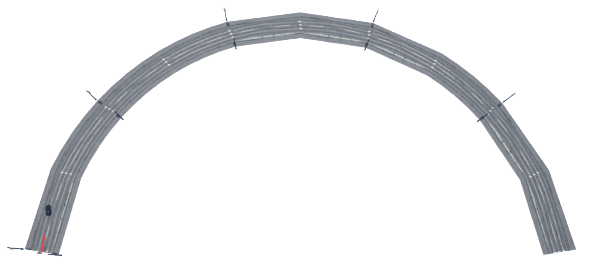
Figure 1: Road geometries used in simulation setup. (The Straight Road at the upper-left, the U-Turn Road at the upper-right and Complete Circuit Track at the bottom.

Another curriculum parameter is the geometry complexity of the track. The track that has the most complex geometry is the hardest track to be learned by the agent. All roads in the simulation are $10$ meters wide and consist of $2$ different lanes. Three tracks in total are used. As it can be seen on Figure 1, they are;

• Straight Road

• U-Turn Road

• Complete Circuit Race Track

To increase the variety of the curriculum learning, weather conditions are added onto these tracks for more realistic settings. The agents which are trained on different weather conditions (such as rain and snow) would learn unique driving capabilities. Note that clear, rainy, and snowy weather conditions are chosen in their maximum value for noteworthy atmospheric ambiances and their effects on the tracks. As a consequence, the curriculum reinforcement learning methodology is implemented on ”Weather Condition” and ”Track Type” combinations.

Each variable set of curriculum training scenarios can be evaluated as separate dimensions in a space. The transition process after each curriculum training phase will take place in the form of a transition from one point in the space to another. Figure 2 can be examined as a representation of the mentioned space and transitions.

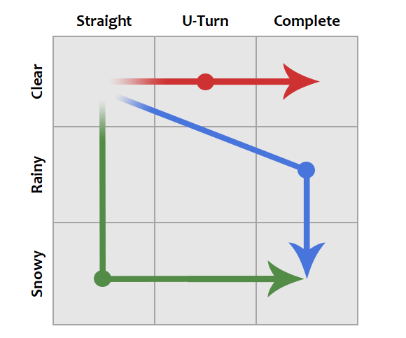
Figure 2: Three example hand-made curriculum scenarios with different road type and weather condition combinations. Each dot represent a combination change in the curriculum. Arrow tips represent the final state.

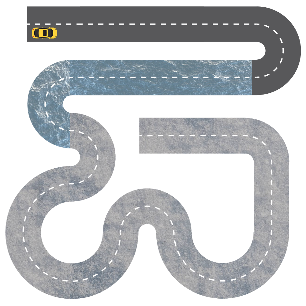
Figure 3: Representation of a full curriculum training scenario, which consists of straight, u-turn, complete roads and clear, rainy, snowy weather conditions, respectively.

An example and a complete curriculum scenario can be seen on Figure 3. The agent observes the phases (Straight, Clean), (U-turn, Clean), (Straight, Rainy), (U-turn, Rainy), (Complete, Snowy) respectively. In the example design, the agent is trained only $1$ iteration on each phase and transferred to the other phase immediately. These iteration numbers will be in thousands in normal applications and the agents can be thought of as spawning back to the beginning of the current phase at the end of each iteration. When the iteration number of each phase is exceeded, the transition to the next phase will be executed.

TABLE II: Training Combinations

Curriculum Scenarios	Phase 1	Phase 2	Phase 3
Scenario 1	Straight (C)	U-Turn (C)	Race Track (C)
Scenario 2	U-Turn (R)	Race Track (R)	Race Track (C)
Scenario 3	Straight (R)	Race Track (R)	Race Track (S)
Scenario 4	Straight (C)	Race Track (R)	Race Track (S)
Scenario 5	Straight (C)	Straight (S)	Race Track (S)

The complete information about training scenarios can be found in Table II. A total of 5 different curriculum scenarios are implemented. Letters C, R and S corresponds to clear, rainy and snowy weather conditions respectively. These route orders are determined by examining the training results without curriculum learning. Most of the cases, the routes are chosen to be ordered from easiest scenarios to hardest. The order of curriculum learning is crucial as the agent has to acquire useful experience in the consecutive tasks [4]. It is seen that, the hardest scenario for the RL agent to solve is complete track scenario with snowy weather condition. So, the goal is to train the agent starting from the easiest track to be learned to the hardest track.

The curriculum training order for each route is illustrated with ascending enumeration. The detailed training scenarios will be discussed in Section V. As stated in [4], the quality of the curriculum learning task is directly dependent on the training order quality of the tracks.

IV-B Reward Structure

To find an optimal policy, the reward structure is crucial for a reinforcement learning problem. In the literature, there are some basic discrete reward functions, but adding road track information and deviation of a vehicle from the road center is important for realistic training. The customized reward function for the training procedures is given in Eq. 3. The reward is calculated at every control step.

$$R=sp\times(cos(\beta)-|sin(\beta)|-tr_{pos})$$ (3)

$sp$ is the speed of the vehicle in $km/h$ obtained from the resultant value of lateral and longitudinal axes speeds. $\beta$ is the angle in radians and it shows the angular deviation of the vehicle heading direction and road central axis. $tr_{pos}$ is the lateral deviation of the vehicle from the road center in meters. Eq. 3 states that if the speed of a vehicle is high, resultant reward gets higher; but the agent would have to minimize the result of $|sin(\beta)|$ and $tr_{pos}$ to get a positive reward. In the reward function, the speed ($sp$) is multiplied with a difference of the road deviation angle’s cosine and sine components to attain members of vehicle’s speed in lateral and longitudinal motion. Another variable in Eq. 3 is $tr_{pos}$ which is the distance of the agent from the central axis in meters. Minus sign of $tr_{pos}$ multiplied with resultant speed of the vehicle makes the negative reward component of total reward calculation. The agent should learn to stay at the center of the road as much as possible because of this negative reward.

IV-C Hyper-parameters

TABLE III: Simulation Parameters

Value Learning Rate, $lr_{value}$	0.0005
Value Learning Rate, $lr_{policy}$	0.0001
Gamma, $\gamma$	0.995
Theta, $\theta$	0.15
Tau, $\tau$	0.001
Alpha, $\alpha$	0.2
Batch Size	64
Buffer Size	100000
State (Input) Size	23

The training is initialized with predetermined hyper-parameters which are shown in Table III. The same hyper-parameters are used in all training cases in this paper for the SAC agent. The state vector consist of $23$ different inputs. $19$ of these inputs come from the laser sensors. The other inputs are related to vehicle position on the track and the current velocity of the vehicle in both X and Y directions.

V Results

At first, the non-curriculum training procedures are carried out on 9 base tracks (3 weather scenarios for 3 road types) as illustrated in Table II. In baseline trainings, the iteration limits are set according to track difficulty levels. The straight road scenarios are trained for $75000$ iterations, U-Turn scenarios are trained for $50000$ iterations and the Circuit Race Track scenarios are trained for $200000$ iterations. After the baseline non-curriculum trainings, a $200000$ iteration limit is decided for the training of curriculum scenarios. In each of 5 different curriculum learning scenarios, 3 different road and weather combinations are used. The first step of all of these curriculum scenarios is one of the baseline trainings that are conducted.

TABLE IV: Baseline Training Results

Road Type / Weather Condition	Straight Road	U-Turn Road	Race Track
Clear	$138,496$	$32,692$	$95,237$
Rainy	$63,155$	$23,571$	$74,476$
Snowy	$39,350$	$16,597$	$70,742$

The baseline training results can be seen in Table IV. As expected, the lowest rewards for all three road types are recorded on snowy environment and the highest reward is achieved in clear weather.

Straight - Clear	It = $75000$ — Rew = $138,496\pm 54\%$
U-Turn - Clear	It = $25000$ — Rew = $42,429\pm 38\%$
Circuit Race Track - Clear	It = $100000$ — Rew = $843,775\pm 18\%$

TABLE V: Results of Scenario 1

U-Turn - Rainy	It = $50000$ — Rew = $23,571\pm 43\%$
Circuit Race Track - Rainy	It = $75000$ — Rew = $63,015\pm 43\%$
Circuit Race Track - Clear	It = $75000$ — Rew = $144,426\pm 24\%$

TABLE VI: Results of Scenario 2

Straight - Rainy	It = $75000$ — Rew = $63,109\pm 43\%$
Circuit Race Track - Rainy	It = $75000$ — Rew = $83,222\pm 56\%$
Circuit Race Track - Snowy	It = $50000$ — Rew = $57,869\pm 27\%$

TABLE VII: Results of Scenario 3

Straight - Clear	It = $75000$ — Rew = $138,496\pm 45\%$
Circuit Race Track - Rainy	It = $75000$ — Rew = $1,117,065\pm 35\%$
Circuit Race Track - Snowy	It = $50000$ — Rew = $1,248,453\pm 29\%$

TABLE VIII: Results of Scenario 4

Straight - Clear	It = $75000$ — Rew = $138,496\pm 47\%$
Straight - Snowy	It = $25000$ — Rew = $143,405\pm 63\%$
Circuit Race Track - Snowy	It = $100000$ — Rew = $597,622\pm 19\%$

TABLE IX: Results of Scenario 5

In the Figure 4, it is possible to see the complete picture of the curriculum learning results.

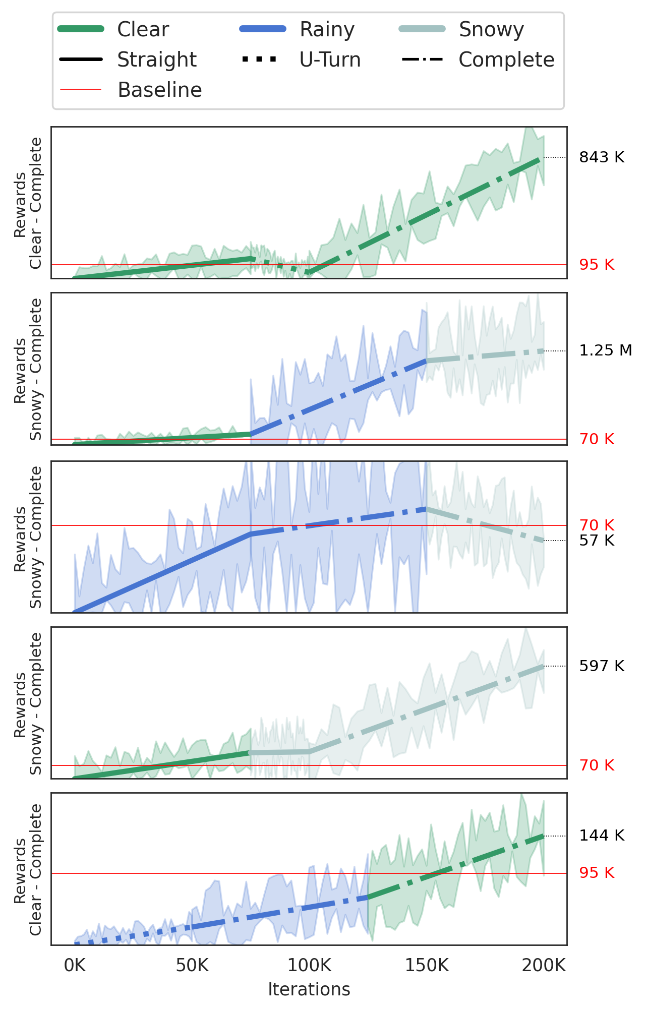
Figure 4: Comparative curriculum learning results. The performances of the models trained with 3 different seeds are shown. Y-Axis represents the rewards, X-Axis represents the environment iterations.

There are 5 rows in the figure and each one of them represents a separate curriculum scenario. Each training phase executed with 3 different pre-defined seeds for the sake of stability. The left side of the figure shows the ending point of the curriculum scenario and right side shows the baseline and curriculum training results. The red lines in the right side shows the baseline training results for that particular curriculum scenario and the black one shows the curriculum training results. Each weather condition is represented with a different color. The clear weather is shown with green, the rainy weather is shown with blue and the snowy weather is shown with celeste color. In the same fashion, all road types are shown with different markers and they can be seen in the upper part of the Figure 4.

VI Discussions

The best results are achieved in a curriculum scenario where the best performing non-curriculum agent used directly in the highest complexity environment. In nearly all of the results, the curriculum learning yielded greater results compared with the non-curriculum results except one case. Using a bad performing non-curriculum agent on a curriculum learning scenario severely hurt the training process and decreased the reward compared with the non-curriculum scenario. This shows that it is crucial to use a good baseline agent in all curricula to achieve better results. The results are affected more by the weather changes than the road complexity.

It might also be helpful to use that insight when deploying an automated curriculum algorithm for decreasing the total time of training. The algorithm that seeks for the optimal transition of the environment variable which has the most impact on reward (snowy to rainy e.g.) would discover optimal curricula faster.

VII Conclusion

In this work, it is showed that training a deep reinforcement learning agent with curriculum learning strategy increases the performance and decreases the overall training time for an autonomous driving agent trained on different weather and road conditions. These results are concluded by developing a structured reinforcement learning system with different road types and weather conditions. The curriculum scenarios on this work consist of different road geometries and weather combinations. It is illustrated that training an RL agent on the relatively simple environment then continuing the the training process of this agent in a more complex environment resulted in a performance boost. During the training process, all parameters kept constant in order to make sure the validity of the experiments. The experimental results demonstrated that an RL agent trained with a curriculum learning structure performed significantly better than an RL agent trained from scratch without a curriculum approach.

VIII Acknowledgements

This work is supported by Istanbul Technical University BAP Grant NO: MOA-2019-42321 and Eatron Technologies, presented at the Workshop on Autonomy at Scale (WS-52), IV2021.

References

- [1] A. Alizadeh, M. Moghadam, Y. Bicer, N. K. Ure, U. Yavas, and C. Kurtulus, “Automated lane change decision making using deep reinforcement learning in dynamic and uncertain highway environment,” 2019 IEEE Intelligent Transportation Systems Conference (ITSC), pp. 1399–1404, 2019.
- [2] A. Ozturk, M. B. Gunel, M. Dal, U. Yavas, and N. K. Ure, “Development of a stochastic traffic environment with generative time-series models for improving generalization capabilities of autonomous driving agents,” pp. 1343–1348, 2020.
- [3] U. S. D. of Transportation, “Federal highway administration road weather management program,” 2021.
- [4] S. Narvekar, B. Peng, M. Leonetti, J. Sinapov, M. E. Taylor, and P. Stone, “Curriculum learning for reinforcement learning domains: A framework and survey,” Journal of Machine Learning Research, vol. 21, no. 181, pp. 1–50, 2020.
- [5] J. L. Elman, “Learning and development in neural networks: The importance of starting small,” 1993.
- [6] Y. Bengio, J. Louradour, R. Collobert, and J. Weston, “Curriculum learning,” p. 41–48, 2009.
- [7] P. Fournier, O. Sigaud, M. Chetouani, and P. Oudeyer, “Accuracy-based curriculum learning in deep reinforcement learning,” CoRR, vol. abs/1806.09614, 2018.
- [8] S. Narvekar and P. Stone, “Learning curriculum policies for reinforcement learning,” 2018.
- [9] T. Matiisen, A. Oliver, T. Cohen, and J. Schulman, “Teacher-student curriculum learning,” 2017.
- [10] W. M. Czarnecki, S. M. Jayakumar, M. Jaderberg, L. Hasenclever, Y. W. Teh, S. Osindero, N. Heess, and R. Pascanu, “Mix&match - agent curricula for reinforcement learning,” CoRR, vol. abs/1806.01780, 2018.
- [11] A. Karpathy and M. van de Panne, “Curriculum learning for motor skills,” 2012.
- [12] A. Graves, M. Bellemare, J. Menick, R. Munos, and K. Kavukcuoglu, “Automated curriculum learning for neural networks,” 2017.
- [13] Y. Sun, J. Cheng, G. Zhang, and H. Xu, “Mapless motion planning system for an autonomous underwater vehicle using policy gradient-based deep reinforcement learning,” 2019.
- [14] J. Zhang and K. Cho, “Query-efficient imitation learning for end-to-end simulated driving,” 2017.
- [15] S. Ross, G. J. Gordon, and J. Bagnell, “No-regret reductions for imitation learning and structured prediction,” 2010.
- [16] “The open racing car simulator.”
- [17] Z. Qiao, K. Muelling, J. M. Dolan, P. Palanisamy, and P. Mudalige, “Automatically generated curriculum based reinforcementlearning for autonomous vehicles in urban environment,” 2018.
- [18] M. Kaushik, V. Prasad, K. M. Krishna, and B. Ravindran, “Overtaking maneuvers in simulated highway driving using deep reinforcement learning,” 2018.
- [19] R. S. Sutton and A. G. Barto, Reinforcement learning: An introduction. MIT press, 2018.
- [20] D. Silver, G. Lever, N. Heess, T. Degris, D. Wierstra, and M. Riedmiller, “Deterministic policy gradient algorithms,” in Proceedings of the 31st International Conference on Machine Learning (E. P. Xing and T. Jebara, eds.), vol. 32 of Proceedings of Machine Learning Research, (Bejing, China), pp. 387–395, PMLR, 22–24 Jun 2014.
- [21] T. Haarnoja, A. Zhou, P. Abbeel, and S. Levine, “Soft actor-critic: Off-policy maximum entropy deep reinforcement learning with a stochastic actor,” in Proceedings of the 35th International Conference on Machine Learning (J. Dy and A. Krause, eds.), vol. 80 of Proceedings of Machine Learning Research, (Stockholmsmässan, Stockholm Sweden), pp. 1861–1870, PMLR, 10–15 Jul 2018.
- [22] “Vehicles — NVIDIA PhysX SDK 3.4.0 documentation.”
- [23] H. B. Pacejka, “Chapter 4 - semi-empirical tire models,” in Tire and Vehicle Dynamics (Third Edition) (H. B. Pacejka, ed.), pp. 149–209, Butterworth-Heinemann.
- [24] A. A. Kordani, O. Rahmani, A. Nasiri, and S. M. Boroomandrad, “Effect of adverse weather conditions on vehicle braking distance of highways,”