Duality and modular symmetry in the quantum Hall effect from Lifshitz holography

Abstract

The temperature dependence of quantum Hall conductivities is studied in the context of the AdS/CMT paradigm using a model with a bulk theory consisting of (3+1)-dimensional Einstein-Maxwell action coupled to a dilaton and an axion, with a negative cosmological constant. We consider a solution which has a Lifshitz like geometry with a dyonic black-brane in the bulk. There is an $Sl(2,{\bm{R}})$ action in the bulk corresponding to electromagnetic duality, which maps between classical solutions, and is broken to $Sl(2,{\bm{Z}})$ by Dirac quantisation of dyons. This bulk $Sl(2,{\bm{Z}})$ action translates to an action of the modular group on the 2-dimensional transverse conductivities. The temperature dependence of the infra-red conductivities is then linked to modular forms via gradient flow and the resulting flow diagrams show remarkable agreement with existing experimental data on the temperature flow of both integral and fractional quantum Hall conductivities.

DIAS-STP-21-05

1 Introduction

The quantum Hall effect (QHE) is a fascinating phenomenon involving a strongly interacting system that exhibits an extensive hierarchy of quantum phase transitions. As a strongly interacting quantum system it is a candidate for testing the ideas of the AdS/CFT correspondence [1] in the context of a (3+1)-dimensional bulk space-time with a (2+1)-dimensional boundary and there has already been a substantial body of work exploring this possibility [4]-[27]. Although the original AdS/CFT conjecture was for large $N$ supersymmetric theories with 4-dimensional boundary it has been applied to non-supersymmetric theories in condensed matter (for a review see [28]). The QHE is not relativistic nor are the different quantum phases of the system described by conformal field theories (CFT’s), but the phase transition between the Hall plateaux are second order and non-relative systems have been considered in the more general framework of geometries with Lifshitz scaling [8] in the AdS/CMT (Condensed Matter Theory) approach (for a review of Lifshitz holography see [9]).

It was observed in [29]-[31] that the QHE has an emergent infra-red modular symmetry relating the different QHE phases and this should be incorporated into any attempt to model the QHE in the AdS/CMT picture. Some steps have already been taken in this direction [11, 10, 18, 33] and these ideas will be explored further here. In this work gradient flow for the $\beta$-functions for the conductivity will be considered within the AdS/CMT framework. Gradient flow in the QHE compatible with modular symmetry was proposed in [34, 35] with potentials that were quasi-holomorphic in the complex conductivity $\sigma=\sigma^{xy}+i\sigma^{xx}$. An anti-holomorphic potential using modular forms was suggested in [36]-[38] and holomorphic potentials were considered in [39]. For a review of the status of modular symmetry in the QHE see [40].

The starting point will be a bulk theory with a dilaton and an axion that enjoys $Sl(2,{\bm{R}})$ symmetry of the classical solutions derived from electromagnetic duality [41]. The strength of the coupling between the dilaton $\phi$ and the axion $\chi$ to the electromagnetic field is determined by a parameter $\lambda$ and they can be combined into a complex field $\tau=\lambda\chi+ie^{-\lambda\phi}$ which we shall call the dilaxion. It will be shown that the infra-red conductivity arising from a bulk solution which contains a dyonic black-brane is related to the complex conjugate of the value of the dilaxion at the event horizon, $\sigma=-\overline{\tau}_{h}$. Quantum effects then break $Sl(2,{\bm{R}})$ to $Sl(2,{\bm{Z}})$, resulting in rational filling fractions, [33]. The black-brane has a Hawking temperature which allows the temperature dependence of the conductivity to be determined from the classical solution and a flow diagram is generated.

Assuming anti-holomorphic gradient flow, with a potential that is holomorphic in $\overline{\sigma}$, and a viable potential function with only one free parameter is constructed using modular invariants. There is a second order phase transition between quantum Hall states with a critical exponent that depends on the free parameter in the potential. The resulting temperature flow of the 2-dimensional conductivity tensor is shown in figure 6, which compares very favourably with the available experimental data [42, 43, 44].

The layout of the paper is as follows. §2 describes the background bulk action and dyonic solutions of the equations of motion are presented in §3. The Dirac quantisation in the bulk, and how it relates to fractional filling factors on the boundary, is discussed in §4. The RG equation for the conductivity is discussed in §5 where it is shown that the DC conductivity is determined by the value of the dilaxion at the event horizon. A discussion of the temperature flow of the DC conductivity is given in §6 and implications of the results are discussed in §7. Some technical details required in the main body of the text are given in three appendices.

2 Einstein-Maxwell-dilaton-axion Lagrangian with a cosmological constant

The starting point is Einstein-Maxwell theory in four dimensional space-time with a dilaton, an axion and a negative cosmological constant. This is interpreted as an effective action action after any charged matter is integrated out and it will suffice for a preliminary investigation of the resulting 2-point correlators. The Lagrangian is

$${\cal L}=\frac{1}{2\kappa^{2}}\bigl{(}{\cal R}-2\Lambda-\partial^{\mu}\phi\partial_{\mu}\phi-e^{2\lambda\phi}\partial^{\mu}\chi\partial_{\mu}\chi\bigl{)}-\frac{1}{4}e^{-\lambda\phi}F_{\mu\nu}F^{\mu\nu}+\frac{1}{4}\lambda\chi F_{\mu\nu}\widetilde{F}^{\mu\nu}$$ (1)

where $\kappa^{2}=8\pi G$, $c=1$, $\lambda$ is a dimensionless parameter, and $\widetilde{F}^{\mu\nu}=\frac{1}{2}\frac{\epsilon^{\mu\nu\rho\sigma}}{\sqrt{-g}}F_{\rho\sigma}$. In terms of the dilaxion field

$${\tau}=\lambda\chi+ie^{-\lambda\phi}$$

and

$$G^{\mu\nu}=e^{-\lambda\phi}F^{\mu\nu}-\lambda\chi\widetilde{F}^{\mu\nu}$$

the Lagrangian is

$${\cal L}=\frac{1}{2\kappa^{2}}({\cal R}-2\Lambda)+\frac{2}{\kappa^{2}\lambda^{2}}\frac{\partial^{\mu}{\tau}\,\partial_{\mu}\overline{\tau}}{({\tau}-\overline{\tau})^{2}}-\frac{1}{4}G^{\mu\nu}F_{\mu\nu}.$$ (2)

Gibbons and Rasheed [41] have shown that, given any solution of the equations of motion of (1), new solutions can be generated by applying an $Sl(2,{\bm{R}})$ symmetry transformation. Define the complex fields

$${\cal F}^{\mu\nu}=F^{\mu\nu}+i\widetilde{F}^{\mu\nu},\qquad{\cal G}^{\mu\nu}=-iG^{\mu\nu}+\widetilde{G}^{\mu\nu}=\overline{\tau}{\cal F}^{\mu\nu}$$

then an $Sl(2,{\bm{R}})$ action is defined on the fields by

$$\begin{pmatrix}{\cal G}\cr{\cal F}\end{pmatrix}\ \longrightarrow\ \begin{pmatrix}{\cal G}^{\prime}\cr{\cal F}^{\prime}\end{pmatrix}=\begin{pmatrix}{a}&{b}\cr{c}&{d}\end{pmatrix}\begin{pmatrix}{\cal G}\cr{\cal F}\end{pmatrix}$$

with

$${\tau}\ \longrightarrow\ {\tau}^{\prime}=\frac{{a}{\tau}+{b}}{{c}{\tau}+{d}}$$ (3)

where ${a}$, ${b}$, ${c}$ and ${d}$ are real and ${a}{d}-{b}{c}=1$, while the metric $g_{\mu\nu}$ is left invariant. If $\bigl{(}F^{\mu\nu},{\tau},g_{\mu\nu}\bigr{)}$ is a solution then this $Sl(2,{\bm{R}})$ action generates a new solution $\bigl{(}(F^{\prime})^{\mu\nu},{\tau}^{\prime},g_{\mu\nu}\bigr{)}$.

The transformation properties of the electric and magnetic fields can be succinctly written using an orthonormal basis $\{e^{0},e^{i}\}$, with $i=1,2,3$, in which

$$E_{i}=-F_{0i}\qquad\mbox{and}\qquad B^{i}=\frac{1}{2}\epsilon^{ijk}F_{jk}=-\frac{1}{2}\epsilon^{0ijk}F_{jk}$$

($\epsilon_{0123}=-e^{0123}=+1$). The complex field

$${\bm{E}}_{i}=E_{i}+iB_{i}$$

transforms as

$${\bm{E}}_{i}\rightarrow{\bm{E}}^{\prime}_{i}=({c}{\tau}+{d}){\bm{E}}_{i}.$$ (4)

The electric charge and total magnetic flux,

$$Q_{e}=\int_{T^{2}}*G,\qquad{Q_{m}}=\int_{T^{2}}F,$$ (5)

transform as

$$\begin{pmatrix}Q_{e}\\ Q_{m}\end{pmatrix}\ \rightarrow\ \begin{pmatrix}a&b\\ c&d\\ \end{pmatrix}\begin{pmatrix}Q_{e}\\ Q_{m}\end{pmatrix}$$ (6)

which is a generalisation of the Witten effect [45].

3 Static, spherically symmetric solutions

It was shown in [46] that there are no static, spherically symmetric solutions of (1) when the cosmological constant is positive, but the present focus will be on the negative case, $\Lambda=-\frac{3}{L^{2}}$. A black-brane solution, with a planar event horizon and negative cosmological constant, was found in [47]. It is a purely electric solution with the metric

$$ds^{2}=-\left(\frac{r}{l}\right)^{2z}\left(1-\left(\frac{r_{h}}{r}\right)^{z+2}\right)dt^{2}+\left(\frac{l}{r}\right)^{2}\frac{dr^{2}}{\left(1-\left(\frac{r_{h}}{r}\right)^{z+2}\right)}+r^{2}(d\vartheta^{2}+d\varphi^{2})$$ (7)

where $r_{h}$, $l$ and $z$ are constants. This metric gives non-relativistic holography with $z$ a temporal scaling exponent. Such Lifshitz-like geometries were proposed in [48, 49] as AdS/CFT models for non-relativistic systems Constant $r$ hypersurfaces at large $r$ are then conformal to 3-dimensional space-times on which the speed of light is $\left(\frac{r}{l}\right)^{z-1}$, [50]. We will use periodic boundary conditions on surfaces of constant $t$ and $r$, in order to keep their area finite, giving them the topology of a torus with area

$${\cal A}_{r}=r^{2}\int_{T^{2}}d\vartheta\wedge d\varphi.$$ (8)

The equations of motion for the action (1) are then satisfied by

$$F_{tr} =-q_{0}\left(\frac{r}{l}\right)^{z+1}$$ (9)

$$e^{-\lambda\phi} =e^{-\lambda\phi_{0}}\left(\frac{l}{r}\right)^{4}$$ (10)

$$\chi =\chi_{0},$$ (11)

with $q_{0}$, $\phi_{0}$ and $\chi_{0}$ constants, provided

$$z =1+\frac{8}{\lambda^{2}}$$ (12)

$$l^{2} =\frac{(z+1)(z+2)L^{2}}{6}$$ (13)

$$q_{0}^{2}e^{-\lambda\phi_{0}} =\frac{6}{\kappa^{2}L^{2}}\frac{(z-1)}{(z+1)}.$$ (14)

$z$ and $l$ are not free, they are fixed in term of $\lambda$ and $L$, and $q_{0}$ and $\phi_{0}$ are not independent. The Lifshitz scaling symmetry is broken by the $r$-dependence of $\phi$, [51]. For large $r$ the Ricci tensor is

$$R_{\mu\nu}\ \rightarrow\ \frac{1}{l^{2}}\begin{pmatrix}z(z+2)\left(\frac{r}{l}\right)^{2z}&0&0&0\\ 0&-(z^{2}+2)\left(\frac{l}{r}\right)^{2}&0&0\\ 0&0&-(z+2)r^{2}&0\\ 0&0&0&-(z+2)r^{2}\\ \end{pmatrix}$$

and the metric is only asymptotically AdS if $z=1$.

Although $F_{tr}$ and $\phi$ diverge asymptotically

$$G_{tr}=-q_{0}e^{-\lambda\phi_{0}}\left(\frac{r}{l}\right)^{z-3},\qquad G^{tr}=q_{0}e^{-\lambda\phi_{0}}\left(\frac{r}{l}\right)^{-(z+1)},$$

the energy density

$$-G^{\mu\nu}F_{\mu\nu}=2q_{0}^{2}e^{-\lambda\phi_{0}}$$

is finite. The pre-factor $e^{-\lambda\phi(r)}$ is like a background electric permittivity, which dies off asymptotically so as to render the energy density in the electric field finite at large $r$, although the electric field itself diverges there.

The total electric charge on the torus can be calculated using Gauss’ law and is independent of $r$,

$$Q_{e}=-q_{0}e^{-\lambda\phi_{0}}l^{2}\int_{T^{2}}d\vartheta\wedge d\varphi$$ (15)

(the normal to the torus is taken to be in the direction of decreasing $r$). There is no magnetic charge and this will be called the electric solution.

3.1 Hawking temperature

The Hawking temperature associate with the metric (7) is

$${T}=\frac{(z+2)\hbar}{4\pi l}\left(\frac{r_{h}}{l}\right)^{z}.$$ (16)

Thus ${T}\rightarrow 0$ smoothly as $r_{h}\rightarrow 0$ and there is no Hawking-Page phase transition associated with this geometry.

The solution fixes $l$ in terms of the Lagrangian parameters $\lambda$ and $L$, but $r_{h}$ is a free parameter which is related to the mass of the black-brane. The area of the event horizon is

$${\cal A}_{h}=\frac{r_{h}^{2}}{l^{2}}{\cal A}_{l},$$ (17)

where

$${\cal A}_{l}=l^{2}\int_{T^{2}}d\vartheta\wedge d\varphi$$ (18)

is a fixed fiducial area, in terms of which the Bekenstein-Hawking entropy is

$$S=\frac{{\cal A}_{h}}{4G\hbar}=\frac{2\pi{\cal A}_{l}r_{h}^{2}}{\kappa^{2}\hbar\,l^{2}}=\frac{2\pi{\cal A}_{l}}{\kappa^{2}\hbar}\left(\frac{4\pi l{T}}{(z+2)\hbar}\right)^{2/z}.$$

From the first law of black hole thermodynamics

$$dM=TdS=T\left(\frac{4\pi{\cal A}_{l}r_{h}}{\kappa^{2}\hbar\,l^{2}}dr_{h}\right)=\frac{(z+2)r_{h}^{z+1}{\cal A}_{l}}{l^{z+3}\kappa^{2}}dr_{h}=d\left(\frac{{\cal A}_{l}r_{h}^{z+2}}{l^{z+3}\kappa^{2}}\right),$$

so

$$M=\frac{{\cal A}_{l}}{\kappa^{2}l}\left(\frac{r_{h}}{l}\right)^{z+2}.$$ (19)

The heat capacity is

$$C_{p}=T\frac{\partial M}{\partial T}=\frac{(z+2)}{z}M=\frac{(z+2)}{z}\frac{{\cal A}_{l}}{\kappa^{2}l}\left(\frac{4\pi lT}{(z+2)\hbar}\right)^{(z+2)/z}>0$$

and the system is thermodynamically stable for any $T>0$, in agreement with the observation above that there is no Hawking-Page phase transition.

For the classical solution to be valid we must ensure that both $l$ and $r_{h}$ are well above the Planck length $L^{2}_{Pl}=\frac{\hbar\kappa^{2}}{8\pi}$,

$$\frac{l^{2}}{\kappa^{2}}\gg\hbar,\qquad\frac{r_{h}^{2}}{\kappa^{2}}\gg\hbar,$$

but this in itself does not restrict $\frac{r_{h}}{l}$. Nevertheless

$$T=\frac{(z+2)}{4\pi}\left(\frac{L_{Pl}}{l}\right)\left(\frac{r_{h}}{l}\right)^{z}T_{Pl},$$

where $T_{Pl}=\frac{\hbar}{L_{Pl}}$ is the Plank temperature so demanding that $T\ll T_{Pl}$ imposes the extra condition

$$\left(\frac{r_{h}}{l}\right)^{z}\ll\frac{l}{L_{Pl}}.$$ (20)

3.2 Dyonic solutions

The $Sl(2,\bm{R})$ action can now be used to generate static, spherically symmetric dyonic solutions from (7)-(11). It is convenient to first change co-ordinates: let $\tilde{t}=\bigl{(}\frac{r_{h}}{l}\bigr{)}^{z}t$, $u=\frac{r_{h}}{r}$, $x=r_{h}d\vartheta$, and $y=r_{h}d\varphi$, so $0\leq u\leq 1$ and event horizon is at $u=1$, the asymptotic region is $u\rightarrow 0$. Then (7) becomes

$$ds^{2}=-\left(1-u^{z+2}\right)\frac{d\tilde{t}\,^{2}}{{u^{2z}}}+\frac{l^{2}}{(1-u^{z+2})}\frac{du^{2}}{u^{2}}+\frac{dx^{2}}{u^{2}}+\frac{dy^{2}}{u^{2}}.$$ (21)

In these variables the electric solution (9), (10) and (11) is

$$F_{\tilde{t}u} =q_{0}\left(\frac{r_{h}}{l}\right)^{2}\frac{l}{u^{z+3}}$$ (22)

$$G_{\tilde{t}u} =q_{0}e^{-\lambda\phi_{0}}\left(\frac{l}{r_{h}}\right)^{2}\frac{l}{u^{z-1}},$$ (23)

$$e^{-\lambda\phi} =e^{-\lambda\phi_{0}}\left(\frac{l}{r_{h}}\right)^{4}u^{4}.$$ (24)

In terms of orthonormal 1-forms

$$e^{0}=\frac{\sqrt{1-u^{z+2}}}{u^{z}}d\tilde{t},\quad e^{1}=\frac{l}{u\sqrt{1-u^{z+2}}}du,\quad e^{2}=\frac{dx}{u},\quad e^{3}=\frac{dy}{u},$$

this purely electric configuration is

$$F=\left(\frac{r_{h}}{l}\right)^{2}\frac{q_{0}}{u^{2}}e^{01},\qquad G=q_{0}\left(\frac{r_{h}}{l}\right)^{2}\zeta u^{2}e^{01},\qquad{\tau}=\lambda\chi_{0}+i\zeta u^{4}$$ (25)

where $e^{01}=e^{0}\wedge e^{1}$ and

$$\zeta=e^{-\lambda\phi_{0}}\left(\frac{l}{r_{h}}\right)^{4}.$$ (26)

Under a $Sl(2,{\bm{R}})$ transformation $\begin{pmatrix}{a}&{b}\\ {c}&{d}\end{pmatrix}$ the metric is unchanged and, from (4), the purely electric configuration (25) is mapped to a configuration with a constant magnetic component,

$$F =q_{0}\left(\frac{r_{h}}{l}\right)^{2}\left(\frac{{d}}{u^{2}}e^{01}-{c}\,\zeta u^{2}e^{23}\right)$$ (27)

$$G =q_{0}\left(\frac{r_{h}}{l}\right)^{2}\left({a}\,\zeta u^{2}e^{01}+\frac{{b}}{u^{2}}e^{23}\right),$$ (28)

while the dilaxion becomes

$${\tau}=\frac{i{a}\zeta u^{4}+{b}+{a}\lambda\chi_{0}}{i{c}\zeta u^{4}\ +{d}+{c}\lambda\chi_{0}}=\frac{i{a}\zeta u^{4}+b_{\chi_{0}}}{i{c}\zeta u^{4}\ +d_{\chi_{0}}}$$ (29)

where $b_{\chi_{0}}=b+{a}\lambda\chi_{0}$ and $d_{\chi_{0}}={d}+c\lambda\chi_{0}$ (with ${a}d_{\chi_{0}}-b_{\chi_{0}}{c}=1$). The dilaton and axion fields are separately

$$e^{-\lambda\phi}=\frac{\zeta u^{4}}{d_{\chi_{0}}^{2}+{c}^{2}\zeta^{2}u^{8}},\qquad\lambda\chi=\frac{b_{\chi_{0}}d_{\chi_{0}}+{a}\,{c}\,\zeta^{2}u^{8}}{d_{\chi_{0}}^{2}+{c}^{2}\zeta^{2}u^{8}}.$$ (30)

Defining $q=q_{0}d$ and $m=-q_{0}\,c\,e^{-\lambda\phi_{0}}$ the Maxwell field strength is

$$F=\left(\frac{r_{h}}{l}\right)^{2}\frac{q}{u^{2}}e^{01}+\left(\frac{l}{r_{h}}\right)^{2}mu^{2}e^{23},$$ (31)

and the full set of coupled equations of motion with (31) and (30) are satisfied in the metric (21) provided

$$\kappa^{2}l^{2}e^{-\lambda\phi_{0}}q^{2} =(z-1)(z+2)\,{d}^{2},$$ (32)

$$\kappa^{2}l^{2}e^{\lambda\phi_{0}}m^{2} =(z-1)(z+2)\,{c}^{2},$$ (33)

$$e^{-\lambda\phi_{0}}q{c}+m{d} =0.$$ (34)

If $\phi_{0}=0$ in the electric solution a non-zero $\phi_{0}$ can be generated by choosing $b=c=0$ and $a=d^{-1}=e^{\lambda\phi_{0}/2}$, and if $\chi_{0}=0$ a constant non-zero topological susceptibility is generated by choosing $c=0$ and $b\neq 0$. Apart from $r_{h}$ there are four parameters in the solution: physically these are $q$, $\phi_{0}$, $m$ and $\chi_{0}$, equivalent to $a$, $b$, $c$ and $d$, but only three of these are independent since $ad-bc=1$.

The total magnetic flux of the solution is

$${Q_{m}}=\int_{T^{2}}F=m\left(\frac{l}{r_{h}}\right)^{2}{\cal A}_{h}=ml^{2}{\mathscr{A}}_{0}$$ (35)

where ${\mathscr{A}}_{0}=\int_{T^{2}}d\vartheta\wedge d\varphi$ is dimensionless. The electric charge is

$$Q_{e}=\int_{T^{2}}*G=-e^{-\lambda\phi_{0}}\left(\frac{l}{r_{h}}\right)^{2}\frac{q{a}}{{d}}{\cal A}_{h}=\frac{m{a}}{{c}}{\cal A}_{l},$$ (36)

where the second equality follows from (34).

If the total charges $Q_{m}$ and $Q_{e}$ are kept constant the magnetic field and charge density are functions of $u$

$$B(u)=\frac{Q_{m}}{{\cal A}_{h}}u^{2}\qquad\mbox{and}\qquad\rho(u)=\frac{Q_{e}}{{\cal A}_{h}}u^{2}.$$

At the event horizon

$$B_{h}=\frac{Q_{m}}{{\cal A}_{l}}\frac{l^{2}}{r_{h}^{2}}=\frac{Q_{m}}{{\cal A}_{l}}\left(\frac{(z+2)\hbar}{4\pi lT}\right)^{2/z}$$ (37)

and

$$\rho_{h}=\frac{Q_{e}}{{\cal A}_{l}}\frac{l^{2}}{r_{h}^{2}}=\frac{Q_{e}}{{\cal A}_{l}}\left(\frac{(z+2)\hbar}{4\pi lT}\right)^{2/z}.$$ (38)

In the quantum Hall effect, with electric charge $e_{0}$ and unit of magnetic flux $\Phi_{0}$, the filling factor is defined to be

$$\nu=\frac{\rho}{e_{0}}\frac{\Phi_{0}}{B}=\frac{Q_{e}}{{Q_{m}}}\frac{\Phi_{0}}{e_{0}}=\frac{{a}}{{c}}\frac{\Phi_{0}}{e_{0}}$$ (39)

and is independent of $u$.

4 Dirac-Schwinger-Zwanziger quantisation

It was observed in [33] that the Dirac-Schwinger-Zwanziger quantisation condition on dyons in the bulk translates to a rational filling factor on the boundary. In the AdS/CFT correspondence gauge symmetries in the bulk correspond to global symmetries on the boundary and the authors of [33] identify the global $U(1)$ on the boundary arising from the bulk $U(1)$ gauge field as being associated with the conservation of composite fermion number in the QHE on the boundary. In Jain’s composite fermion picture of the QHE [52], [53] the statistical gauge field generates a ‘fictitious’ background magnetic field which is quantised and concentrated in $\delta$-function magnetic magnetic vortices.

For the general dyonic solution (31)-(34) the total magnetic flux through the torus $T^{2}$, at fixed $t$ and $u$, is (35). If there is a quantum unit of magnetic flux $\Phi_{0}$ then ${Q_{m}}$ will be integer multiple of $\Phi_{0}$

$${Q_{m}}=N_{m}\Phi_{0},\qquad N_{m}\in{\bf Z}.$$

Mathematically one could set $\Phi_{0}=2\pi$ so that

$$N_{m}=\frac{1}{2\pi}\int_{T^{2}}F$$

is the first Chern number of a $U(1)$ line bundle over the torus. In physical units $\Phi_{0}=\frac{2\pi\hbar}{e}$, where $e$ is the charge of the electron, might seem natural and indeed this would be correct for a quantum Hall system, but there are other possibilities. In a superconductor, for example, Cooper pairs have charge $e_{0}=2e$ and the unit of magnetic flux is $\frac{h}{2e}$. Of course $\frac{\Phi_{0}}{e_{0}}$ is dimensionless and in the following we shall use units with $\frac{e_{0}^{2}}{h}=\frac{n^{2}e^{2}}{h}=1$, where $n=1$ for quantum Hall systems and $n=2$ for superconductors. The unit of electric charge is then $e_{0}=ne$ and the unit of magnetic flux is $\Phi_{0}=\frac{h}{ne}$, with $e_{0}\Phi_{0}=h$ and $\frac{e_{0}}{\Phi_{0}}=1$, in these units $e_{0}=\Phi_{0}=\sqrt{2\pi\hbar}$.

The total electric charge $Q_{e}$ is a multiple of $e_{0}$

$$Q_{e}=N_{e}e_{0},\qquad N_{e}\in{\bf Z},$$

and, from the Dirac quantisation condition,

$$\frac{Q_{e}{Q_{m}}}{2\pi\hbar}=N_{e}N_{m}\in{\bf Z}.$$

Eliminating $q$ and $m$ in favour of ${d}$ and ${c}$ using (32)-(34), equations (35) and (36) give

$$Q_{m}=-\frac{{c}\,e^{-\lambda\phi_{0}/2}}{\eta},\qquad Q_{e}=-\frac{{a}\,e^{-\lambda\phi_{0}/2}}{\eta},$$ (40)

where

$$\eta=\frac{\kappa l}{{\cal A}_{l}}\frac{1}{\sqrt{(z-1)(z+2)}}.$$ (41)

Let $N$ be the greatest common divisor of $N_{e}$ and $N_{m}$, where the sign chosen so that $N_{e}=-N{\mathbf{a}}$ and $N_{m}=-N{\mathbf{c}}$, with ${\mathbf{a}}$ and ${\mathbf{c}}$ mutually prime. Then

$$Q_{m}=-N{\mathbf{c}}\Phi_{0},\qquad Q_{e}=-N{\mathbf{a}}\,e_{0}$$

with

$${\mathbf{a}}=\frac{{a}e^{-\lambda\phi_{0}/2}}{\sqrt{2\pi\hbar}}\left(\frac{1}{\eta N}\right),\qquad{\mathbf{c}}=\frac{{c}e^{-\lambda\phi_{0}/2}}{\sqrt{2\pi\hbar}}\left(\frac{1}{\eta N}\right).$$

If we further define

$${\mathbf{b}}={b}e^{\lambda\phi_{0}/2}\eta N\sqrt{2\pi\hbar},\qquad{\mathbf{d}}={d}e^{\lambda\phi_{0}/2}\eta N\sqrt{2\pi\hbar}$$ (42)

then

$$\begin{pmatrix}{a}&{b}\\ {c}&{d}\end{pmatrix}=\begin{pmatrix}{\mathbf{a}}&{\mathbf{b}}\\ {\mathbf{c}}&{\mathbf{d}}\end{pmatrix}\begin{pmatrix}e^{\lambda\phi_{0}/2}\eta N\sqrt{2\pi\hbar}&0\\ 0&\bigl{(}e^{\lambda\phi_{0}/2}\eta N\sqrt{2\pi\hbar}\bigr{)}^{-1}\end{pmatrix}$$ (43)

with ${\mathbf{a}}{\mathbf{d}}-{\mathbf{b}}{\mathbf{c}}=1$. Setting $\begin{pmatrix}{\mathbf{a}}&{\mathbf{b}}\\ {\mathbf{c}}&{\mathbf{d}}\end{pmatrix}=\begin{pmatrix}1&0\\ 0&1\end{pmatrix}$ in (43) equation (29) then gives the electric dilaxion field to be

$$\tau=2\pi\hbar N^{2}\eta^{2}e^{\lambda\phi_{0}}(\lambda\chi_{0}+i\zeta u^{4}),$$

so we set

$$e^{-\lambda\phi_{0}}=2\pi\hbar N^{2}\eta^{2}=\frac{2\pi\hbar\kappa^{2}}{(z-1)(z+2)l^{2}}\left(\frac{N}{{\mathscr{A}}_{0}}\right)^{2},$$ (44)

this is does not reduce the number of parameters in the solution, we are just trading $\phi_{0}$ for $\frac{N}{{\mathscr{A}}_{0}}$. The dilaxion associated with any magnetic monopole or dyon solution compatible with the Dirac quantisation condition is now obtained from

$${\tau}=\lambda\chi_{0}+i\zeta u^{4}$$

by acting on it by a general element of $\Gamma(1)$.

Note that an immediate consequence of Dirac-Schwinger-Zwanziger quantisation is that the filling fraction

$$\nu=\frac{{a}}{{c}}=\frac{{\mathbf{a}}}{{\mathbf{c}}}$$ (45)

is a rational number.

In summary the general quantised dyonic solution in terms of the integers ${\mathbf{a}}$, ${\mathbf{b}}$, ${\mathbf{c}}$ and ${\mathbf{d}}$ satisfying ${\mathbf{a}}{\mathbf{d}}-{\mathbf{b}}{\mathbf{c}}=1$, is

$$Q_{e} =-N{\mathbf{a}}\,e_{0},\qquad\qquad\quad{Q_{m}}=-N{\mathbf{c}}\Phi_{0},$$ (46)

$$F_{\tilde{t}u} =\left(\frac{r_{h}}{l}\right)^{2}\frac{q\,l}{u^{z+3}},\qquad\ F_{xy}=m\left(\frac{l}{r_{h}}\right)^{2},$$ (47)

$$q ={\mathbf{d}}\left(\frac{(z-1)(z+2)}{2\pi\hbar\kappa^{2}l^{2}}\frac{{\cal A}_{l}}{N}\right)e_{0},\qquad m=-{\mathbf{c}}\left(\frac{N\Phi_{0}}{{\cal A}_{l}}\right),$$ (48)

$${\tau} =\left(\frac{{\mathbf{a}}(\lambda\chi_{0}+i\zeta u^{4})+{\mathbf{b}}}{{\mathbf{c}}(\lambda\chi_{0}+i\zeta u^{4})+{\mathbf{d}}}\right)\frac{e_{0}}{\Phi_{0}},$$ (49)

with $\zeta=2\pi\hbar N^{2}\eta^{2}\left(\frac{l}{r_{h}}\right)^{4}$ and $e_{0}=\Phi_{0}=\sqrt{2\pi\hbar}$.

The full solution is acted on by $Sl(2,{\bm{Z}})$ but, apart from the sign of $F_{\mu\nu}$, the dyon solution is invariant under

$$\begin{pmatrix}{\mathbf{a}}&{\mathbf{b}}\\ {\mathbf{c}}&{\mathbf{d}}\end{pmatrix}\rightarrow-\begin{pmatrix}{\mathbf{a}}&{\mathbf{b}}\\ {\mathbf{c}}&{\mathbf{d}}\end{pmatrix},$$

and the dilaxion transforms under the modular group $\Gamma(1)\approx Sl(2,{\bf Z})/{\bf Z}_{2}$. Note also that, while $m$ is proportional to ${\mathbf{c}}$ and $q$ is proportional to ${\mathbf{d}}$, the electric charge is determined by ${\mathbf{a}}$ and not by ${\mathbf{d}}$, because of the Witten effect.

The dimensionless parameter $\zeta$ depends on the Hawking temperature of the system (16). Since

$$\frac{r_{h}}{l}=\left\{\frac{4\pi lT}{(z+2)\hbar}\right\}^{1/z}$$

we can write

$$\zeta=\left(\frac{T_{*}}{T}\right)^{4/z}=\Theta^{-4/z}\quad\mbox{with}\quad\Theta=\frac{T}{T_{*}}$$

where

$$T_{*} =\left(\frac{(z+2)\hbar}{4\pi l}\right)\left(2\pi\hbar N^{2}\eta^{2}\right)^{z/4}$$

$$=\left(\frac{z+2}{4\pi}\right)\left(\frac{N^{2}}{4{\mathscr{A}}_{0}^{2}(z-1)(z+2)}\right)^{z/4}\left(\frac{L_{Pl}}{l}\right)^{(z+2)/2}T_{Pl}.$$

In the next section $T_{*}$ will be related to the critical temperature of a second order phase transition and, if it is to be interpreted as a physical temperature, we should therefore ensure that $T_{*}\ll T_{Pl}$ which requires

$$\frac{N^{2}}{{\mathscr{A}}_{0}^{2}}\ll\left(\frac{l}{L_{Pl}}\right)^{2(z+2)/z}.$$

At the same time $T\ll T_{Pl}$ implies that

$$\Theta^{4/z}\ll\frac{{\mathscr{A}}_{0}^{2}}{N^{2}}\left(\frac{l}{L_{Pl}}\right)^{2(z+2)/z}.$$

5 Conductivities

In the AdS/CMT paradigm the boundary of space-time is associated with a $2+1$ dimensional system which we shall interpret in the present context as a strongly coupled electron system. This is perhaps rather radical for the classical dyon solution solution presented in the previous section, as the bulk space-time is not even asymptotically AdS, but we shall see that interesting results emerge notwithstanding (our model can be viewed as the near horizon limit of an asymptotically AdS model [10]). The presence of temporal scaling, with $z>1$, results in a boundary theory which is non-relativistic and the non-zero magnetic field generated by the dyon sets the stage for the analysis of the quantum Hall effect.

The conductivity tensor is obtained in linear response from a variation

$$\delta E_{\alpha}(\tilde{t},u)=e^{-i\widetilde{\omega}\tilde{t}}\delta\widetilde{E}_{\alpha}(u),\qquad\delta B(\tilde{t},u)^{\alpha}=e^{-i\widetilde{\omega}\tilde{t}}\delta\widetilde{B}^{\alpha}(u)$$ (50)

in the transverse electric and magnetic fields (${\alpha}=x,y$) which satisfies the linearised equations of motion in the chosen background. We work in a gauge in which the potential for the field variation is

$$\delta A_{\alpha}(\tilde{t},u)=e^{-i\widetilde{\omega}\tilde{t}}\delta\widetilde{A}_{\alpha}(u),$$

where it is understood that $\delta\widetilde{A}_{\alpha}(u)$ depends on $\widetilde{\omega}$. A static electric field can be modelled either with

$$\delta A_{\alpha}(\tilde{t},u)=-(\delta E_{\alpha}^{0})\tilde{t}+\delta\widetilde{A}_{\alpha}(u),$$ (51)

provided $\delta E_{\alpha}^{0}$ is independent of $u$, or by allowing $\delta\widetilde{A}_{\alpha}$ to have a pole at $\widetilde{\omega}=0$ with residue $-i\delta E_{\alpha}^{0}$.

The electric field generates a current

$$\delta J^{\alpha}=\sigma^{{\alpha}{\beta}}\delta E_{\alpha}\qquad\Rightarrow\qquad\sigma^{{\alpha}{\beta}}=\frac{\delta J^{\alpha}}{\delta E_{\beta}}$$

where

$$\delta E_{\alpha}=-\delta F_{\tilde{t}{\alpha}}=i\widetilde{\omega}\delta\widetilde{A}_{\alpha},\qquad\delta B^{\alpha}=\frac{\epsilon^{\tilde{t}u{\alpha}{\beta}}}{\sqrt{-g}}\delta F_{u{\beta}}=-\frac{1}{l}u^{z+3}\epsilon^{{\alpha}{\beta}}\delta\widetilde{A}^{\prime}_{\beta}.$$

The current at any given $u$ is obtained from the action by varying $\delta\widetilde{A}_{\alpha}(u)$ keeping the potential at the event horizon fixed,

$$\widetilde{J}^{\alpha}(u)=\frac{\delta S[A]}{\delta\widetilde{A}^{\alpha}(u)}$$

from which the transverse conductivity tensor is [55]

$$\sigma^{{\alpha}{\beta}}(\widetilde{\omega},u)=\frac{1}{i\widetilde{\omega}}\frac{\delta^{2}S[A]}{\delta\widetilde{A}^{\alpha}(u)\delta\widetilde{A}^{\beta}(u)},$$ (52)

If we wish to take quantum corrections into account the classical action $S[A]$ should be replaced by an effective quantum action $S_{eff}[A]$, but the philosophy of the AdS/CFT correspondence is that a classical solution in the bulk corresponds to a strongly interacting quantum theory on the boundary so this conductivity will be interpreted as the conductivity of a strongly interacting quantum system at scale $r=\frac{r_{h}}{u}$. Bulk quantum corrections would be a further refinement.

It will be convenient to use complex co-ordinates and define

$$\sigma_{\pm} =\sigma^{xy}\pm i\sigma^{xx}$$ (53)

$$\delta J_{\pm} =\delta J^{x}\pm i\delta J^{y}$$ (54)

$${\delta\cal E}_{\pm} =\delta E_{x}\pm i\delta E_{y}$$ (55)

$${\delta\cal B}_{\pm} ={\delta\cal B}^{x}\pm i{\delta\cal B}^{y}=\frac{(1-u^{z+2})}{u^{2(z+1)}}(\delta B^{x}\pm i\delta B^{y}).$$ (56)

The pre-factor in (56) ensures that, in an orthonormal basis, where the electric and magnetic fields have components $\delta E_{i}$ and $\delta B^{i}$ with $i=2,3$,

$${\delta\cal E}_{\pm}=\frac{\sqrt{1-u^{z+2}}}{u^{z+1}}(\delta E_{2}\pm i\delta E_{3}),\quad{\delta\cal B}_{\pm}=\frac{\sqrt{1-u^{z+2}}}{u^{z+1}}(\delta B^{2}\pm i\delta B^{3}),$$ (57)

so ${\delta\cal E}_{\pm}$ and ${\delta\cal B}_{\pm}$ have the same weight.

Adapting the analysis in [55] to include the dilaxion it is shown in appendix B that the conductivity is

$$\sigma_{\pm}(u)=e^{-\lambda\phi}\frac{{\delta\cal B}_{\pm}}{{\delta\cal E}_{\pm}}-\lambda\chi,$$ (58)

in units with $\frac{e_{0}^{2}}{h}=1$.

5.1 DC conductivity

When $\widetilde{\omega}=0$ the DC conductivity (58) can be obtained directly from Maxwell’s equations for $\delta F_{\mu\nu}$ in the dyon background,

$$\partial_{\mu}\bigl{(}\sqrt{-g}\,e^{-\lambda\phi}\delta F^{\mu\nu}\bigr{)}-\frac{\lambda}{2}\epsilon^{\mu\nu\sigma\lambda}(\partial_{\mu}\chi)\delta F_{\sigma\lambda}=0.$$ (59)

For static, homogeneous variations all fields are independent of time and independent of $x$, and $y$ so, we only need consider transverse co-ordinates $\nu={\alpha}=x$ or $y$ for which

$$\bigl{(}\sqrt{-g}\,e^{-\lambda\phi}\delta F^{u{\alpha}}\bigr{)}^{\prime}+\lambda\epsilon^{{\alpha}{\beta}}\chi^{\prime}\delta F_{\tilde{t}{\beta}}=0$$

where ${}^{\prime}=\frac{d}{du}$. For the DC conductivity

$$\delta F_{\tilde{t}{\beta}}=-\delta E^{0}_{\beta}$$

are constant and Maxwell’s equations reduce to

$$\bigl{(}e^{-\lambda\phi}{\delta\cal B}_{\pm}-\lambda\chi{\delta\cal E}^{0}_{\pm}\bigr{)}^{\prime}=0.$$ (60)

We use ingoing boundary conditions at the event horizon (this is the source of dissipation in the AdS/CFT paradigm [54]). With Eddington-Finkelstein co-ordinates

$$v_{\pm}=\tilde{t}\pm\int\sqrt{\frac{g_{uu}}{-g_{\tilde{t}\tilde{t}}}}\,du=\tilde{t}\pm l\int\frac{u^{z-1}du}{(1-u^{z+2})}$$

ingoing boundary conditions at $u=1$ require that

$$\left.\partial_{v_{+}}(\delta A_{\pm})\right|_{u=1}=0$$ (61)

so, near $u=1$,

$$\mp iu^{z-1}l{\delta\cal B}_{\pm}=(1-u^{z+2})\delta A_{\pm}^{\prime}\ \approx-l\partial_{\tilde{t}}(\delta A_{\pm})=l({\delta\cal E}^{0}_{\pm})$$ (62)

where $\delta A_{\pm}=\delta A_{x}\pm i\delta A_{y}$.

Integrating Maxwell’s equations (60)

$$\frac{e^{-\lambda\phi}\bigl{(}1-u^{z+2}\bigr{)}}{lu^{z-1}}(\delta A_{\pm})^{\prime}\pm i\lambda\chi({\delta\cal E}^{0}_{\pm}) =C_{\pm}$$ (63)

$$\Leftrightarrow\qquad e^{-\lambda\phi}({\delta\cal B}_{\pm})-\lambda\chi({\delta\cal E}^{0}_{\pm}) =\pm iC_{\pm}$$ (64)

with $C_{\pm}=C^{x}\pm iC^{y}$ constants. Hence the DC conductivity

$$\sigma_{\pm}=e^{-\lambda\phi}\frac{{\delta\cal B}_{\pm}}{{\delta\cal E}^{0}_{\pm}}-\lambda\chi=\pm i\frac{C_{\pm}}{{\delta\cal E}^{0}_{\pm}}.$$

is independent of $u$. The constants $C_{\pm}$ can be obtained from Maxwell’s equations in the dyon background,

$$\zeta(1-u^{z+2})\delta\widetilde{A}_{\pm}^{\prime}=\bigl{\{}C_{\pm}(d_{\chi_{0}}^{2}+{c}^{2}\zeta^{2}u^{8})\mp i(b_{\chi_{0}}d_{\chi_{0}}+{a}{c}\zeta^{2}u^{8})({\delta\cal E}^{0}_{\pm})\bigr{\}}lu^{z-5}$$ (65)

and the ingoing boundary condition (62) enforces

$$C_{\pm} =\pm i\left(\frac{b_{\chi_{0}}d_{\chi_{0}}+{a}{c}\zeta^{2}}{d_{\chi_{0}}^{2}+{c}^{2}\zeta^{2}}\right){\delta\cal E}^{0}_{\pm}+\left(\frac{\zeta}{d_{\chi_{0}}^{2}+{c}^{2}\zeta^{2}}\right){\delta\cal E}^{0}_{\pm}$$

$$\Rightarrow\qquad C_{+} =C_{-}^{*}=i\,\overline{\tau}_{h}{\delta\cal E}^{0}_{+}.$$

where ${\tau}_{h}$ is the dilaxion at the event horizon. Hence the DC conductivities are given by the value of the dilaxion field at the horizon,

$$\sigma_{+}=-\overline{\tau}_{h},\qquad\sigma_{-}=-{\tau}_{h}.$$ (66)

Maxwell’s equations can also be solved to give ${\delta\cal B}_{\pm}(u)$ explicitly in the static case,

$$(1-u^{z+2})\delta\widetilde{A}_{\pm}^{\prime} =\frac{(d_{\chi_{0}}\pm i\zeta{c})(d_{\chi_{0}}\mp i{c}\zeta u^{8})}{(d_{\chi_{0}}^{2}+\zeta^{2}{c}^{2})}\,u^{z-5}l({\delta\cal E}^{0}_{\pm})$$

$$\Rightarrow\qquad{\delta\cal B}_{\pm} =\pm i\,\frac{(d_{\chi_{0}}\pm i\zeta{c})(d_{\chi_{0}}\mp i{c}\zeta u^{8})}{u^{4}(d_{\chi_{0}}^{2}+{c}^{2}\zeta^{2})}({\delta\cal E}^{0}_{\pm}).$$ (67)

Note that, although equation (67) implies that ${\delta\cal B}_{\pm}$ diverges as $1/u^{4}$ as $u\rightarrow 0$, in an orthonormal basis (57)

$$\delta B^{i}\sim u^{z-3},$$

which is finite for $z\geq 3$. Demanding that the energy density in the magnetic field perturbation

$$\frac{e^{-\lambda\phi}}{2}({\delta\cal B}_{i})^{2}\approx u^{4}u^{2(z-3)}$$

is finite as $u\rightarrow 0$ in a local inertial reference frame gives the weaker condition $z\geq 1$.

5.2 AC conductivity

For oscillating perturbations Maxwell’s equations (59) give us

$$\pm\frac{\widehat{\omega}u^{z-1}}{(1-u^{z+2})}({\delta\cal E}_{\pm})+(e^{-\lambda\phi}{\delta\cal B}_{\pm})^{\prime}-\lambda\chi^{\prime}({\delta\cal E}_{\pm})=0,$$ (68)

where $\widehat{\omega}=l\widetilde{\omega}$.

Consequently the conductivity is no longer independent of $u$, but instead

$$\sigma_{\pm}^{\prime}=-e^{-\lambda\phi}\left(\frac{{\delta\cal B}_{\pm}{\delta\cal E}_{\pm}^{\prime}}{{\delta\cal E}_{\pm}^{2}}\right)\mp\frac{\widehat{\omega}u^{z-1}}{(1-u^{z+2})}=-\left(\sigma_{\pm}+\lambda\chi\right)\left(\frac{{\delta\cal E}_{\pm}^{\prime}}{{\delta\cal E}_{\pm}}\right)\mp\frac{\widehat{\omega}u^{z-1}}{(1-u^{z+2})}.$$

However ${\delta\cal E}_{\pm}^{\prime}$ can be determined from the equations of motion and a radial RG equation for $\sigma_{\pm}$ can be derived. The technical details are left to an appendix, B.1, where the equation in a general dyonic background is derived using the techniques of [55], [56] and [57]. The result is given in equation B.1 (132),

$$\pm\widehat{\omega}u^{4-z}(1-u^{z+2})u\frac{d\sigma_{\pm}}{du}= \ 4\zeta(z-1)(z+2)u^{2(4-z)}(1-u^{z+2})\left({c}\sigma_{\pm}+{{a}}\right)^{2}$$

$$\hskip 20.0pt-\widehat{\omega}^{2}(d_{\chi_{0}}^{2}+{c}^{2}\zeta^{2}u^{8})\bigl{(}\sigma_{\pm}+{\tau}\bigr{)}\bigl{(}\sigma_{\pm}+\overline{\tau})$$ (69)

(recall that $\zeta=e^{-\lambda\phi_{0}}\frac{l^{4}}{r^{4}_{h}}$, for $SL(2,{\bf R})$). Although $\chi_{0}$ can be absorbed into a re-definition of $b$ and $d$ for $Sl(2,{\bf R})$ this is not the case for $Sl(2,{\bf Z})$ after Dirac quantisation).

Interpreting the classical radial equation of motion as an RG equation was suggested in [58], [59] and the relation to the $c$-theorem was studied in [60], [61]. This version of the RG equation is obtained by expressing the radial equation of motion as a Riccati equation, [62]-[68]. An alternative formulation uses the radial Hamilton-Jacobi equation [69]-[71] (for the Hamilton-Jacobi equation in the context of Lifshitz geometry see [9]) and a Wilsonian approach was developed in [72]-[75] (it was argued in [76] that the classical radial equation of motion and the Wilsonian method are equivalent). For our purposes the Riccati equation is the most convenient form.

Ingoing boundary conditions at the event horizon give the same constraint as in the DC case (62),

$${\delta\cal B}_{\pm}=\pm i{\delta\cal E}_{\pm},$$

at $u=1$, so $\sigma_{\pm}|_{u=1}=-\bar{\tau}_{h}$ , but equation (69) already has this boundary condition encoded into it when $\widehat{\omega}\neq 0$, the boundary condition at $u=1$ is no longer at our discretion for $\widehat{\omega}>0$, inflowing boundary conditions are necessarily required.

Note however that equation (69) implies that $\sigma_{\pm}\rightarrow-\frac{{a}}{{c}}=-\nu$ as $\widehat{\omega}\rightarrow 0$, for $0<u<1$, the limits $u\rightarrow 1$ and $\widehat{\omega}\rightarrow 0$ do not commute and the $\widehat{\omega}\rightarrow 0$ limit of the AC conductivity determine by (69) is not the same as the DC conductivity derived in §5.1.

5.2.1 Analysis of the conductivity

The solutions of the general equation (69) are related by

$$\sigma_{+}(-{b},-{c})=-\sigma_{-}({b},{c}),$$

which generalises an observation in [55], so the Hall conductivity is

$$\sigma_{H}=\sigma^{xy}=\frac{1}{2}(\sigma_{+}+\sigma_{-})=\frac{1}{2}\bigl{(}\sigma_{+}({b},{c})-\sigma_{+}(-{b},-{c})\bigr{)}$$

and the Ohmic conductivity is

$$\sigma_{\Omega}=\sigma^{xx}=\frac{1}{2i}(\sigma_{+}-\sigma_{-})=\frac{1}{2i}\bigl{(}\sigma_{+}({b},{c})+\sigma_{+}(-{b},-{c})\bigr{)}.$$

A full analysis of the solutions of (69) requires numerical integration which will not be pursued here, but certain limits are amenable to an analytic approach:

• We expect a cyclotron resonance with damping, [55, 57]. An approximation to the cyclotron resonance can be found provided $\widehat{\omega}$ is small and the second term on the right-hand side of (69) can be ignored. The analytic solution in this approximation is immediate,

  $$\frac{1}{{c}({c}\sigma_{\pm}+{a})}=\mp\frac{4\zeta(z-1)(z+2)u^{4-z}}{(4-z)\widehat{\omega}}+const,\qquad z\neq 4.$$

  For $\sigma_{+}$ the boundary condition at $u=1$ is

  $$\sigma_{+}|_{u=1}=-\overline{\tau}_{h}=-\left(\frac{b_{\chi_{0}}-i{a}\zeta}{d_{\chi_{0}}-i{c}\zeta}\right),$$

  (recall $b_{\chi_{0}}=b+{a}\lambda\chi_{0}$ and $d_{\chi_{0}}={d}+{c}\lambda\chi_{0}$). The solution is

  $$\sigma_{+}=\frac{(4-z)i({a}\zeta+ib_{\chi_{0}})\widehat{\omega}-4{a}\zeta(z-1)(z+2)(1-u^{4-z})}{(4-z)(d_{\chi_{0}}-i{c}\zeta)\widehat{\omega}+4{c}\zeta(z-1)(z+2)(1-u^{4-z})},\qquad z\neq 4$$ (70)

  (for $z=4$, $\lim_{z\rightarrow 4}\bigl{(}\frac{1-u^{4-z}}{4-z}\bigr{)}=-\ln u$).

  To check the range of validity of the approximation, substitute the solution (70) into the right-hand side of (69) and check when the first term dominates the second. Near $u=1$ let $u=1-\epsilon$ and $1-u^{4-z}\approx(4-z)\epsilon$ then the approximation is good provided $\zeta\epsilon\ll 1$ and $\zeta\widehat{\omega}\ll 1$.

  There is a resonance at

  $$\widehat{\omega}_{*}=-\frac{4{c}\zeta(z-1)(z+2)(1-u^{4-z})}{(4-z)({d}_{\chi_{0}}-i{c}\zeta)}.$$

  The Hawking temperature (16) was calculated in §3.1 in terms of $t$ in (7), so $e^{i\omega t}=e^{i\widetilde{\omega}\tilde{t}}$ with $\omega=\frac{4\pi l\widetilde{\omega}T}{(z+2)\hbar}$ and

  $$\widehat{\omega}=\frac{(z+2)\hbar\omega}{4\pi T},$$

  so the resonance corresponds to

  $$\omega_{*}=-\frac{16\pi T{c}\zeta(z-1)(1-u^{4-z})}{\hbar(4-z)(d_{\chi_{0}}-i{c}\zeta)}=\omega_{0}-i\Gamma.$$

  with frequency and damping

  $$\omega_{0} =-\frac{16\pi{c}d_{\chi_{0}}T\zeta(z-1)(1-u^{4-z})}{\hbar(4-z)(d_{\chi_{0}}^{2}+{c}^{2}\zeta^{2})}$$ (71)

  $$\Gamma =\frac{16\pi{c}^{2}T\zeta^{2}(z-1)(1-u^{4-z})}{\hbar(4-z)(d_{\chi_{0}}^{2}+{c}^{2}\zeta^{2})}.$$ (72)

  Since $\Gamma<0$ for $z>4$ there is an instability in the system for such values of $z$ and we shall therefore assume that $1\leq z\leq 4$ from now on.

  Furthermore $\zeta\propto T^{-4/z}$ so both $\omega_{0}$ and $\Gamma$ vanish as $T\rightarrow 0$ but the ${\bm{Q}}$-factor

  $${\bm{Q}}=\frac{|\omega_{0}|}{2\Gamma}=\frac{1}{2\zeta}\left|\frac{d_{\chi_{0}}}{{c}}\right|,$$

  which is independent of $u$, decreases as the temperature is decreased, because $\omega_{0}$ vanishes faster than $\Gamma$.

  A similar phenomenon is seen by continuing to Euclidean time. The Hawking temperature can be derived by requiring that there is no conical singularity in the geometry in Euclidean time which in turn imposes an imaginary periodicity in real time, $t\rightarrow t\rightarrow+\frac{i\hbar}{T}$. But a magnetic system with cyclotron frequency $\omega_{B}$ also has periodicity $\frac{2\pi}{\omega_{B}}$ in real time and combining these gives periodicity

  $$t\ \rightarrow\ t+\frac{2\pi}{\omega_{B}}+\frac{i\hbar}{T}.$$

  This suggests defining a complex frequency $\omega_{*}$ via

  $$\frac{2\pi}{\omega_{*}}=\frac{2\pi}{\omega_{B}}+\frac{i\hbar}{T}\quad\Rightarrow\quad\frac{\omega_{*}}{2\pi}=\frac{\omega_{B}}{2\pi}\left(\frac{1-i\left(\frac{\hbar\omega_{B}}{2\pi T}\right)}{1+\left(\frac{\hbar\omega_{B}}{2\pi T}\right)^{2}}\right)$$ (73)

  giving frequency and damping

  $$\omega_{0}=\frac{\omega_{B}}{1+\left(\frac{\hbar\omega_{B}}{2\pi T}\right)^{2}},\qquad\Gamma=\frac{\left(\frac{\hbar\omega_{B}^{2}}{2\pi T}\right)}{1+\left(\frac{\hbar\omega_{B}}{2\pi T}\right)^{2}}$$ (74)

  with $\bm{Q}$-factor

  $${\bm{Q}}=\frac{2\pi T}{\hbar\omega_{B}}.$$

  The damping decreases as the temperature is lowered, as one would expect, but ${\bm{Q}}$ also decreases as $T$ is lowered is because the resonance frequency falls faster than the damping.

  Going back to (71) and (72) the situation near the event horizon is rather similar, at least at small temperatures where $\zeta$ is large. If the magnetic field is held fixed

  $$c\,\zeta\propto\frac{\omega_{B}}{T^{2/z}}.$$

  Let

  $$\frac{c\,\zeta}{d}=\frac{K}{2\pi}\frac{\hbar\omega_{B}}{T^{2/z}},$$

  with $K$ a constant, and approach the event horizon by choosing
  $\epsilon\approx\frac{1-u^{4-z}}{4-z}=\frac{\pi lT^{2/z}}{2K\hbar(z-1)(z+2)}$ and lowering the temperature. Then

  $$\omega_{0}=\frac{\omega_{B}}{1+K^{2}\Bigl{(}\frac{\hbar\omega_{B}}{2\pi T^{2/z}}\Bigr{)}^{2}},\qquad\Gamma=\frac{K\Bigl{(}\frac{\hbar\omega_{B}^{2}}{2\pi T^{2/z}}\Bigr{)}}{1+K^{2}\Bigl{(}\frac{\hbar\omega_{B}}{2\pi T^{2/z}}\Bigr{)}^{2}}$$ (75)

  the same as (74) if $z=2$ and $K=1$.

• For small $\widehat{\omega}\ll\widehat{\omega}_{0}$ an approximate solution of (69) is (see [57] for more details)

  $$\sigma_{+}=\begin{cases}\frac{-(b_{\chi_{0}}d_{\chi_{0}}+{a}{c}\zeta^{2})+i\zeta}{d_{\chi_{0}}^{2}+{c}^{2}\zeta^{2}},&u=1;\\ -\frac{a}{c},&u<1.\end{cases}$$

  and this is an increasingly better approximation as $\widehat{\omega}\rightarrow 0$.

• Exactly at $u=1$ it is immediate from (69) that, for any non-zero $\widehat{\omega}$, the AC conductivity is

  $$\sigma_{+}=-\overline{\tau}_{h}=\frac{-(b_{\chi_{0}}d_{\chi_{0}}+{a}{c}\zeta^{2})+i\zeta}{d_{\chi_{0}}^{2}+{c}^{2}\zeta^{2}},$$

  the same as the DC conductivity (66).

• As $u\rightarrow 0$, if $z<4$,

  $$\sigma_{+}\rightarrow-\overline{\tau}_{u=0}=-\frac{b_{\chi_{0}}}{d_{\chi_{0}}}$$

  for any finite non-zero $\widehat{\omega}$.

In summary the DC conductivity is independent of $u$,

$$\sigma_{+}^{DC}=\left(\frac{-{a}{c}\zeta^{2}-b_{\chi_{0}}d_{\chi_{0}}+i\zeta}{{c}^{2}\zeta^{2}+d_{\chi_{0}}^{2}}\right).$$ (76)

In general the AC conductivity will depend on $u$ and will require numerics to analyse, but for $\widehat{\omega}\ll\widehat{\omega}_{0}$ it reduces to a step function

$$\sigma_{+}^{AC}= \left(\frac{-{a}{c}\zeta^{2}-b_{\chi_{0}}d_{\chi_{0}}+i\zeta}{{c}^{2}\zeta^{2}+d_{\chi_{0}}^{2}}\right), \mbox{for}\ u=1$$ (77)

$$\sigma_{+}^{AC}= -\frac{{a}}{{c}}, \ \mbox{for}\ 0<u<1$$ (78)

$$\sigma_{+}^{AC}= -\frac{b_{\chi_{0}}}{d_{\chi_{0}}}, \mbox{for}\ u=0.$$ (79)

6 Temperature flow in the infra-red

Since the infra-red conductivity is $\sigma_{+}=-\overline{\tau}|_{u=1}$ the conductivity transforms the same way as the dilaxion under an $Sl(2,{\bm{R}})$ transformation

$$\sigma_{\pm}=-\overline{\tau}_{h}\quad\rightarrow\quad-\left(\frac{a\overline{\tau}_{h}+b}{c\overline{\tau}_{h}+d}\right)=\left(\frac{a\sigma_{\pm}-b}{-c\sigma_{\pm}+d}\right).$$ (80)

Invoking the Dirac quantisation condition in the bulk

$$\sigma=-\overline{\tau}|_{u=1}=\frac{({\mathbf{b}}+{\mathbf{a}}\lambda\chi_{0})\Theta^{4/z}-i{\mathbf{a}}}{i{\mathbf{c}}-({\mathbf{d}}+{\mathbf{c}}\lambda\chi_{0})\Theta^{4/z}}$$ (81)

at the event horizon (we can drop the $\pm$ subscript when $\widehat{\omega}=0$, since then $\sigma=\sigma_{+}$ and $\overline{\sigma}=-\sigma_{-}$ and the only difference between $\sigma_{+}$ and $\sigma_{-}$ is the sign of the Hall conductivity $\sigma_{H}$, in the following $\sigma$ is $\sigma_{+}$). In the purely electric case, ${\mathbf{a}}={\mathbf{d}}=1$, ${\mathbf{b}}={\mathbf{c}}=0$,

$$\sigma=-\lambda\chi_{0}+i\Theta^{-4/z},$$ (82)

with $-\frac{1}{2}\leq\lambda\chi_{0}\leq\frac{1}{2}$, and and the Ohmic conductivity diverges as $T\rightarrow 0$, which would be normal behaviour of a conductor in the absence of impurities. When $T$ is increased the Ohmic resistance grows as $T^{4/z}$, giving a power law with exponent $1\sim 4$ for $4\geq z\geq 1$. Conversely in the purely magnetic case, ${\mathbf{a}}={\mathbf{d}}=0$, ${\mathbf{b}}=-{\mathbf{c}}=1$,

$$\sigma=\frac{\lambda\chi_{0}\Theta^{8/z}+i\Theta^{4/z}}{1+\lambda^{2}\chi_{0}^{2}\Theta^{8/z}},$$ (83)

both the Ohmic and the Hall conductivities tend to zero as $T\rightarrow 0$.

$Sl(2,{\bm{Z}})$ is generated by ${\bm{S}}:\sigma\rightarrow-1/\sigma$ and ${\bm{T}}:\sigma\rightarrow\sigma+1$. In particular $\Theta=1$, $\chi_{0}=0$ is a fixed point under $S$-duality, with critical temperature $T_{*}$, and in the dual phase $\sigma\rightarrow 0$ as $T\rightarrow 0$ for a background with a magnetic charge but no electric charge. This fixed point is similar to the one discussed in [77] [78], in [79] [80] it was interpreted as being due to a superconductor-insulator phase transition arising from Bose condensation of vortices, in which the insulating phase is a Hall insulator.

For $-\frac{1}{2}\leq\lambda\chi_{0}\leq\frac{1}{2}$, $S$-duality places the critical temperature on the boundary of the fundamental domain, where $|\sigma|=1$, at $\Theta=\left(\frac{1}{1-\lambda^{2}\chi_{0}^{2}}\right)^{z/4}$, so the maximum critical temperature is at $\lambda\chi_{0}=\pm\frac{1}{2}$ where $T=\bigl{(}\frac{4}{3}\bigr{)}^{z/4}T_{*}$.

However we now have an apparent paradox. In the classical solution the metric is not affected by $Sl(2,{\bm{R}})$ transformations, in particular $r_{h}$ and hence $T$ are invariant. They should therefore be invariant under $\Gamma(1)$ and yet ${\bm{S}}$ interchanges large and small temperatures. To resolve this we note that $T\rightarrow\infty$ is not accessible to the classical solution as we must constrain $T\ll T_{Pl}$ and we consider two possible strategies:

• Eliminate ${\bm{S}}$ and only allow sub-groups of $\Gamma(1)$ that do not contain ${\bm{S}}$.

• Retain ${\bm{S}}$ but keep $T\leq T_{*}$.

We shall examine these two possibilities in turn, exploring the second one first.

6.1 Retain ${\bm{S}}$ but keep $T\leq T_{*}$

With the superconductor-insulator transition in mind use the electric solution (${\mathbf{a}}={\mathbf{d}}=1$, ${\mathbf{b}}={\mathbf{c}}=0$, $\sigma=-\lambda\chi_{0}+i\Theta^{-4/z}$, $-\frac{1}{2}\leq\chi_{0}\leq\frac{1}{2}$) above the green semi-circular arc bounding the lower edge of the fundamental domain in figure 1, which flows up to the superconductor as $T\rightarrow 0$, and use the magnetic solution (${\mathbf{a}}={\mathbf{d}}=0$, $-{\mathbf{b}}={\mathbf{c}}=1$, $\sigma=\frac{\lambda\chi_{0}\Theta^{8/z}+i\Theta^{4/z}}{1+\lambda^{2}\chi_{0}^{2}\Theta^{8/z}}$) below the green arc, flowing to the Hall insulator as $T\rightarrow 0$. This point of view resonates with the introduction of the complex frequency in (73). Continuing time into the complex plane, complex periodicity suggests defining

$${\cal T}=T_{*}\left(\frac{2\pi}{\omega_{B}}+\frac{i\hbar}{T},\right)$$ (84)

as a Teichmüller parameter for a torus. There is then an $Sl(2,{\bm{Z}})$ action

$${\cal T}\rightarrow\frac{{\mathbf{a}}{\cal T}+{\mathbf{b}}}{{\mathbf{c}}{\cal T}+{\mathbf{d}}}$$

on this temporal torus. If $T\ll\hbar\omega_{B}$ (a necessary condition to access the hierarchy of phases in the QHE) then ${\cal T}\approx\frac{i\hbar}{T}$ and ${\bm{S}}:{\cal T}\rightarrow-\/{\cal T}$ has a fixed point at the critical temperature $\Theta=1$.

The idea is then that different filling fractions $\frac{{\mathbf{a}}}{{\mathbf{c}}}$ label different quantum phases and the flow lines in the fundamental domain $({\mathbf{a}}={\mathbf{d}}=1$, ${\mathbf{c}}={\mathbf{b}}=0)$ are mapped between different phases by the action of $\Gamma(1)$. Temperature flow lines, arising from varying $r_{h}$ in the fundamental domain, with $-\frac{1}{2}\leq\lambda\chi_{0}\leq\frac{1}{2}$ fixed, are shown in figure 1. As the temperature is reduced there are repulsive fixed points at $\sigma=e^{i\pi/3}$, and its images under $\Gamma(1)$ (red circles); attractive fixed points at all rational numbers on the real axis (half-integral values are shown in green), as well as at $Im(\sigma)\rightarrow i\infty$; and saddle points at $\sigma=i$, and its images (blue). The flow looks a little confused on the green lines, which are phases boundaries, but this will be resolved momentarily.

Of course the other flow direction could have been chosen, nothing in the mathematical analysis dictates which direction to use: the direction is chosen on physical grounds, to make the superconductor in the electric phase attractive as $T\rightarrow 0$. Different classical bulk solutions are being used to represent different phases of the 2-dimensional quantum system.

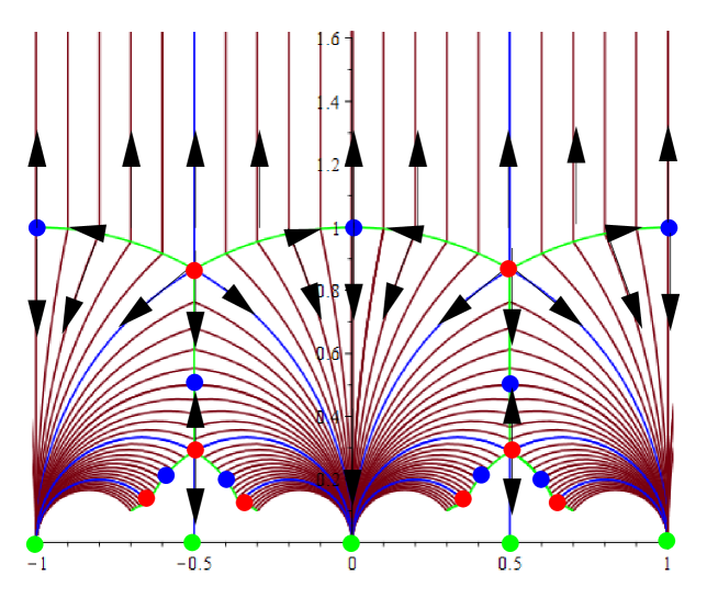
Figure 1: Temperature flow of the conductivity on the event horizon obtained from tiling the upper-half conductivity plane, replicating the fundamental domain using $\Gamma(1)$ symmetry (arrows in direction of decreasing temperature). The green lines indicate phase boundaries, blue circles are saddle points and the red circles are purely repulsive fixed points. Green circles are purely attractive fixed points as $T\rightarrow 0$ (there are attractive fixed points at every rational number on the real axis, but only half-integral values are shown in the figure). The vertical strip $-\frac{1}{2}\leq\sigma^{xy}\leq\frac{1}{2}$ above the green circular arc between $e^{-i\pi/3}$ and $e^{i\pi/3}$, bounded by the vertical blue lines, is a fundamental domain of $\Gamma(1)$.

6.1.1 Gradient flow for $\Gamma(1)$

We now take up the suggestion in [36] that this flow might be derivable as gradient flow with an anti-holomorphic potential. In a conductor or a superconductor the temperature flow of the conductivity is driven by the fact that there is an underlying electron coherence length that depends on the temperature and the conductivity depends on the temperature via the coherence length. In general we can define a flow function resulting from changing the electron coherence length via a change in the temperature as

$$T\frac{d\sigma}{dT}=T\frac{d\xi}{dT}\frac{d\sigma}{d\xi}.$$

Changes in the coherence length length generate a vector field in the conductivity plane

$$\beta(\sigma,\bar{\sigma})=\xi\frac{d\sigma}{d\xi}$$

and, under a modular transformation $\sigma\rightarrow\frac{{\mathbf{a}}\sigma+{\mathbf{b}}}{{\mathbf{c}}\sigma+{\mathbf{d}}}$,

$$\beta(\sigma,\bar{\sigma})\rightarrow\frac{\beta(\sigma,\bar{\sigma})}{({\mathbf{c}}\sigma+{\mathbf{d}})^{2}}.$$ (85)

If this flow is derivable from a potential $\overline{V}(\sigma,\bar{\sigma})$ then

$$\beta(\sigma,\bar{\sigma})=G^{\sigma\bar{\sigma}}\partial_{\bar{\sigma}}\overline{V}(\sigma,\bar{\sigma})$$ (86)

with $G_{\sigma\bar{\sigma}}$ a hermitian metric on the conductivity plane. There is of course a natural candidate for an $Sl(2,{\bm{R}})$ invariant metric and that is

$$G_{\sigma\bar{\sigma}}=\frac{1}{(Im\sigma)^{2}}.$$

The proposal in [36] is that the potential be anti-holomorphic $\overline{V}(\bar{\sigma})$. Under a modular transformation

$$Im\sigma\rightarrow\frac{Im\sigma}{|{\mathbf{c}}\sigma+{\mathbf{d}}|^{2}}$$

so

$$G^{\sigma\bar{\sigma}}\rightarrow\frac{G^{\sigma\bar{\sigma}}}{|{\mathbf{c}}\sigma+{\mathbf{d}}|^{4}}$$

and (86) will have the transformation property (85) if

$$\overline{V}(\bar{\sigma})\rightarrow({\mathbf{c}}\bar{\sigma}+{\mathbf{d}})^{2}\,\overline{V}(\bar{\sigma}),$$ (87)

i.e. $1/V(\sigma)$, the complex conjugate of $1/\overline{V}(\bar{\sigma})$, is a modular form of weight $-2$.

This severely restricts the form of the potential as there is a theorem [81] that any modular form $\Phi_{-2}(\sigma)$ of weight -2 can be written in terms of Klein’s $J$-invariant as

$$\Phi_{-2}(\sigma)=\frac{P(J)}{Q(J)}\frac{1}{J^{\prime}}$$

where $P(J)$ and $Q(J)$ are polynomials in $J$ and $J^{\prime}=\frac{dJ}{d\sigma}$. We shall therefore investigate using $V(\sigma)=\{\Phi_{-2}(\phi)\}^{-1}$ as a potential.

Under this assumption the flow commutes with the $\Gamma(1)$ action and fixed points of $\Gamma(1)$, i.e. points in the $\sigma$-plane that are left invariant by at least one non-trivial element of $\Gamma(1)$, are necessarily fixed points of the flow,

$$\sigma_{*}=\frac{{\mathbf{a}}\sigma_{*}+{\mathbf{b}}}{{\mathbf{c}}\sigma_{*}+{\mathbf{d}}}\quad\Rightarrow\quad\beta(\sigma_{*},\bar{\sigma}_{*})=\frac{\beta(\sigma_{*},\bar{\sigma}_{*})}{({\mathbf{c}}\sigma_{*}+{\mathbf{d}})^{2}}\quad\Rightarrow\quad\beta(\sigma_{*},\bar{\sigma}_{*})=0\quad\mbox{or}\quad\infty.$$

There are three points in the fundamental domain that are left invariant by some element of $\Gamma(1)$: $\sigma_{1,*}=i\infty$, $\sigma_{2,*}=e^{i\pi/2}$ and $\sigma_{3,*}=e^{i\pi/3}$, with $J$ taking values $+\infty$, $1$ and $0$, respectively at these three points. In fact $J$ is real and monotonically increasing from $0$ to $1$ as $\sigma$ goes from $e^{i\pi/3}$ to $e^{i\pi/2}$, along the unit circular arc, and then increases from $1$ to $\infty$ along the vertical line as $\sigma$ runs from $i$ to $i\infty$.

There can be more fixed points though, a zero of $Q(J)$ would give $\beta=0$ and a zero of $P(J)$ would give a divergent $\beta$. The simplest assumption is that there are no fixed points of the flow other than the fixed points of $\Gamma(1)$. A property of $J$ is that it takes all possible complex values once and only once in the fundamental domain of $\Gamma(1)$, so if $P(J)$ and $Q(J)$ are to have no zeros other than at $e^{i\pi/3}$, $i$ and $i\infty$ it must be the case that

$$\frac{{Q(J)}}{{P(J)}}=-\overline{C}J^{m}(J-1)^{n}$$

for some pair of if integers $m$ and $n$, with $C$ a constant. Furthermore $m$ and $n$ are restricted by the form of the classical solution of the equations of motion.

Consider the purely electric solution (82) with $\chi_{0}=0$ and

$$\sigma=i\Theta^{-4/z},$$

above the fixed point $\Theta=i$ with $\Theta\leq 1$. The metric on this line is

$$G_{\sigma\bar{\sigma}}=\Theta^{8/z}$$

so

$$\beta=-\frac{C\overline{J}^{m}(\overline{J}-1)^{n}}{\Theta^{8/z}}\frac{d\,\overline{J}}{d\bar{\sigma}}=\xi\frac{d\sigma}{d\xi}.$$

Now consider the three types of fixed point:

• $\bm{\sigma_{*,1},\sigma\rightarrow i\infty}$: in terms of $q=e^{i\pi\sigma}$, $J$ has the small $q$ expansion

  $$J=\frac{1}{1728}\Bigl{(}q^{-2}+744+196884q^{2}+21493760\,{q}^{4}+O\bigr{(}{q}^{6}\bigr{)}\Bigr{)}$$

  so as $\Theta\rightarrow 0$

  $$\beta\ \approx\ -\frac{2\pi iC\Theta^{-8/z}}{(1728)^{m+n+1}}e^{\frac{2\pi(m+n+1)}{\Theta^{4/z}}}$$

  giving

  $$\xi\frac{d\Theta^{-4/z}}{d\xi}\ \approx\ -\frac{2\pi C\Theta^{-8/z}}{(1728)^{m+n+1}}e^{\frac{2\pi(m+n+1)}{\Theta^{4/z}}}$$

  (clearly $C$ must be real for $\xi$ to be real).

  If the $\beta$-function is to be analytic as $T\rightarrow 0$, $m$ and $n$ must be restricted by the constraint $m+n+1=0$. This gives

  $$\xi\approx\xi_{0}\exp\left({\frac{\Theta^{4/z}}{2\pi C}}\right)\ \rightarrow\ \xi_{0}\quad\mbox{as}\quad\Theta\rightarrow 0$$ (88)

  and the coherence length is a non-zero constant as $T\rightarrow 0$.

• $\bm{\sigma_{*,2}}=i$: for $\sigma=i+\epsilon$ with $\epsilon$ small

  $$J\approx 1-k\epsilon^{2},$$

  with $k=\frac{3}{64\pi^{4}}\left\{\Gamma\left(\frac{1}{4}\right)\right\}^{8}\approx 14.37$, so

  $$\beta\approx 2Ck\bar{\epsilon}(-k\bar{\epsilon}^{2})^{n},$$

  since $G^{\sigma\bar{\sigma}}=1+O(\epsilon)$. Demanding that $\beta$ is finite at $\sigma=i$ restricts us to $n\geq 0$. Now let ${\tt t}=1-\Theta$ be the reduced temperature near the critical point, with $0\leq{\tt t}\leq 1$, then

  $$\bar{\epsilon}=-\frac{4i{\tt t}}{z}$$

  and

  $$\beta\approx-2iCk^{n+1}\left(\frac{4{\tt t}}{z}\right)^{2n+1}.$$

  Together with

  $$\beta=\xi\frac{d{\tt t}}{d\xi}\frac{d\sigma}{d{\tt t}}=\frac{4i}{z}\left(\xi\frac{d{\tt t}}{d\xi}\right)$$

  this gives

  $$\frac{1}{\xi}\frac{d\xi}{d{\tt t}} \approx-\frac{1}{2Ck^{n+1}}\left(\frac{z}{4}\right)^{2n}{\tt t}^{-(2n+1)}$$

  $$\Rightarrow\quad\ln\xi \approx\begin{cases}\frac{1}{4nC}\left(\frac{z}{4}\right)^{2n}k^{-(n+1)}{\tt t}^{-2n},&n\neq 0;\\ -\frac{1}{2kC}\ln{\tt t},&n=0.\end{cases}$$

  $n=0$ gives the scaling behaviour

  $$\xi\approx A{\tt t}^{-\nu^{\prime}}$$

  with $A$ a constant and critical exponent

  $$\nu^{\prime}=\frac{1}{2kC}=\frac{32\pi^{4}}{3C\bigl{\{}\Gamma(\frac{1}{4})\bigr{\}}^{8}}.$$

• $\bm{\sigma_{*,3}=e^{i\pi/3}}$: what of the third fixed point at $\sigma_{3,*}=e^{i\pi/3}$? Near $e^{i\pi/3}$, with $\sigma=e^{i\pi/3}+\epsilon^{\prime}$, $J$ vanishes as

  $$J\approx-ik^{\prime}(\epsilon^{\prime})^{3}$$

  with $k^{\prime}$ a positive constant. The metric takes the value $G_{\sigma\bar{\sigma}}=\frac{4}{3}$ giving

  $$\beta\approx\frac{9C}{4}(-1)^{n+1}\bigl{(}e^{i\pi/2}k^{\prime}\bigr{)}^{m+1}(\bar{\epsilon}\,^{\prime})^{3m+2}.$$

  Demanding that $\beta$ is finite at $\epsilon^{\prime}=0$ would constrain $m$ to be positive, but requiring $\beta$ to be analytic at all three fixed points gives three incompatible conditions, $m+n=-1$, $n\geq 0$ and $m\geq 0$. We do not yet have a physical interpretation of $\epsilon^{\prime}$ so we shall keep $m+n+1=0$ and $n\geq 0$ and allow $m<0$. The marginal case is $n=0$, $m=-1$, in which case there is a simple pole in $\beta$ at $\sigma_{*,3}$.

  On the unit circular arc from $\sigma_{*,2}$ to $\sigma_{*,3}$, $\sigma=e^{i(\frac{\pi}{3}+\psi)}$ with $0\leq\psi\leq\frac{\pi}{6}$, $J$ is real and lies in the range $1\geq J\geq 0$. Close to $e^{i\pi/3}$, where $\psi\ll 1$,

  $$\epsilon^{\prime}\approx e^{5i\pi/6}\psi$$

  and

  $$\xi\frac{d\psi}{d\xi}\approx-\frac{9C}{4\psi}\quad\Rightarrow\quad\xi\approx\tilde{\xi}_{0}e^{-\frac{2\psi^{2}}{9C}}.$$

In summary the behaviour of $\xi$ near the fixed points is

$$\xi\sim\begin{cases}\xi_{0}\exp\left(\frac{\Theta^{4/z}}{2\pi C}\right),&\Theta\rightarrow 0;\\ A{\tt t}^{-\nu\,^{\prime}},&\Theta\rightarrow 1,\ \mbox{with}\ \nu\,^{\prime}=\frac{32\pi^{4}}{3C\bigl{\{}\Gamma(\frac{1}{4})\bigr{\}}^{8}};\\ \tilde{\xi}_{0}\exp\left(-\frac{2\psi^{2}}{9C}\right),&\sigma=e^{i(\pi/3+\psi)}\rightarrow e^{i\pi/3}.\end{cases}$$ (89)

The classical solution in the bulk does not give us $\psi$ as a function of $T$, but a consistent picture emerges if $\psi$ is monotonic in $T$ and $T$ increases monotonically from $T_{*}$ to infinity along the circular arc connecting the two fixed points $e^{i\pi/2}$ and $e^{i\pi/3}$. The hypothesis of gradient flow has resolved the ambiguity across the green arc of points in figure 1 and replaced it with a separatrix between the two adjoining phases.

On the upper segment of the imaginary axis, $\sigma=i\Theta^{-4/z}$ for $\Theta$ in the range $1\geq\Theta\geq 0$ while $J$ is real and lies in the range $1\leq J(\sigma)<\infty$ and we can invert the explicit formula for $J(\sigma)$, (146) in appendix C) to plot $\Theta$ in this range as a function of $J$ (this is shown in figure 2).

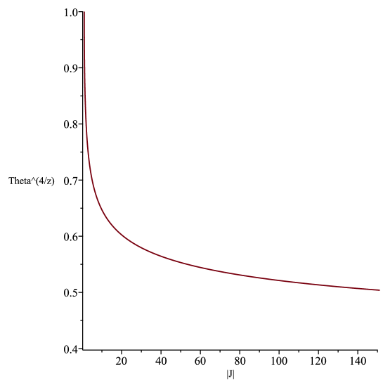
Figure 2: Temperature as a function of $|J|$ for $|J|\geq 1$ along the imaginary axis, with $\Gamma(1)$ flow. $\Theta$ drops monotonically from unity at $|J|=1$ to zero as $|J|\rightarrow\infty$. Asymptotically $\Theta^{4/z}\approx\frac{2\pi}{\ln|J|}$. This assumes that the classical solution gives the correct temperature dependence along the imaginary axis.

Now the temperature, and hence $\Theta$, depends only on the metric and not on any $Sl(2,{\bm{R}})$ transformation of the classical solution, and so $\Theta$ should be modular invariant. Suppose therefore that $\Theta$ can be extended to a real function $\Theta(J,\overline{J})$ over the whole of the fundamental domain, and by extension using $\Gamma(1)$ to the whole upper-half complex plane. If $\Theta$ is a monotonic function of $|J|$ everywhere then flow lines can be obtained by varying $|J|$, keeping its argument $\Psi$ fixed. With $J=|J|e^{i\Psi}$ and $m=-1$, $n=0$

$$\xi\frac{d\sigma}{d\xi}=-C(\sigma^{xx})^{2}\frac{d\ln\overline{J}}{d\overline{\sigma}}=-\frac{C}{2}\frac{d(\ln|J|^{2})}{d\overline{\sigma}}+iC(\sigma^{xx})^{2}\xi\frac{d\Psi}{d\xi}.$$

Now

$$\Psi=\tan^{-1}\left\{\frac{i(\overline{J}-J)}{(\overline{J}+J)}\right\}\qquad\Rightarrow\qquad\frac{d\Psi}{d\sigma}=-\frac{i}{2J}\frac{dJ}{d\sigma}$$

and

$$\xi\frac{d\Psi}{d\xi} =\xi\frac{d\sigma}{d\xi}\frac{d\Psi}{d\sigma}+\xi\frac{d\,\overline{\sigma}}{d\xi}\frac{d\Psi}{d\,\overline{\sigma}}$$

$$=-C(\sigma^{xx})^{2}\left\{\frac{d\ln\overline{J}}{d\overline{\sigma}}\left(-\frac{i}{2J}\right)\left(\frac{dJ}{d\sigma}\right)+\frac{d\ln J}{d\sigma}\left(\frac{i}{2\overline{J}}\right)\left(\frac{d\overline{J}}{d\overline{\sigma}}\right)\right\}$$

$$=0$$

if $C$ is real. Thus for real $C$ the argument of $J$ is indeed constant along the flow lines. Furthermore

$$\xi\frac{d|J|^{2}}{d\xi} =\xi\frac{d\overline{\sigma}}{d\xi}\frac{d|J|^{2}}{d\overline{\sigma}}+\xi\frac{d\sigma}{d\xi}\frac{d|J|^{2}}{d\sigma}$$

$$=-C(\sigma^{xx})^{2}\left\{\frac{d\ln J}{d\sigma}\frac{d|J|^{2}}{d\overline{\sigma}}+\frac{d\ln\overline{J}}{d\overline{\sigma}}\frac{d|J|^{2}}{d\sigma}\right\}$$

$$=-2C\left(\sigma^{xx}\left|\frac{dJ}{d\sigma}\right|\right)^{2}$$

$$\Rightarrow\qquad\xi\frac{d\ln|J|}{d\xi} =-C\left(\sigma^{xx}\left|\frac{d\ln|J|}{d\sigma}\right|\right)^{2}$$

hence $|J|$ is indeed a monotonically decreasing function of $\ln\xi$. The temperature flow can therefore be visualised as lines of constant $\Psi$ in the conductivity plane and these are plotted in figure 3 (this figure is obtained using the logic in [39, 82]).

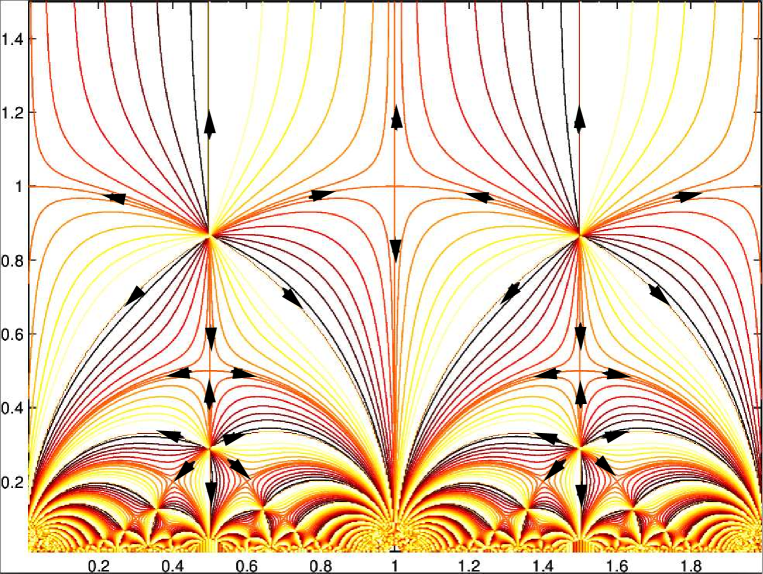
Figure 3: Temperature flow of the conductivity on the event horizon for $\Gamma(1)$ symmetry, assuming it is generated by varying $|J|$, keeping $\arg(J)$ fixed. The diagram is obtained simply by plotting lines of constant $\arg(J)$, which are represented by different colours from red ($\Psi=0$) through black ($\Psi=\pi$) to yellow.

$J$ is real on the segment of the unit circle centered on the origin that connects these two fixed points and decreases from 1 at $\sigma_{*,2}$ to to 0 at $\sigma_{*,3}$, as $\Theta$ rises from $1$ to infinity. Thus the full temperature range $0\leq\Theta<\infty$ is re-instated in a self-consistent flow. The fixed point at $e^{i\pi/3}$ is a sink in the high temperature direction that takes the theory out of its domain of validity as the temperature is increased, in the AdS/CMT paradigm this would suggest that quantum effects become significant in the bulk and the 2-D quantum system becomes weakly coupled at $\sigma^{i\pi/3}$.

It is not necessary to know the function $\Theta(J,\overline{J})$ explicitly in order to plot figure 3, it can be any monotonic function of $|J|$. The classical solution only gives $\Theta$ for $\arg(J)=0$, and even then only for $J\geq 1$. It is a strong assumption that $\Theta(|J|,\Psi)$ is monotonic in $|J|$ everywhere and that the temperature flow is obtained by varying $|J|$, but the picture that emerges under these assumptions is at least consistent. In the next section similar assumption are made for the sub-group $\Gamma_{0}(2)\subset\Gamma(1)$ and give very good agreement with experimentally measured flows.

6.2 Eliminate ${\bm{S}}$

Another way of obtaining a consistent temperature flow is to eliminate ${\bm{S}}$ and consider a subgroup of $\Gamma(1)$. For example we could consider the set of elements generated by repeated application of $\bm{STS}$ and $\bm{T}$, but $(\bm{ST})^{3}=1$ so $(\bm{STS}){\bm{T}}(\bm{STS})=\bm{S}$ and $\bm{S}$ re-appears. However $\bm{ST}^{2}\bm{S}$ and $\bm{T}$ do generate a group — the subgroup $\Gamma_{0}(2)$ of $\Gamma(1)$, and this is one option, but there are others [11], [83] (appendix §C collects together some relevant facts about level 2 subgroups of $\Gamma(1)$ and their modular forms).

The group $\Gamma_{0}(2)$ has two fixed points on the imaginary axis, at $\sigma=i\infty$ and $\sigma=0$, but the $\Gamma(1)$ fixed point at $\sigma_{2,*}$ is gone. The temperature flow diagram generated by taking the purely magnetic solution

$$\sigma=-\lambda\chi_{0}+i\Theta^{4/z}$$

in the fundamental domain of $\Gamma_{0}(2)$, with $-1\leq\lambda\chi_{0}\leq 0$ fixed, and mapping it around with elements of $\Gamma_{0}(2)$ is shown in figure 4. $\Gamma_{0}(2)$ has a third fixed point at $\sigma_{*}=\frac{1}{2}(1+i)$, left invariant by $\begin{pmatrix}1&-1\\ 2&-1\end{pmatrix}$ which reflects the green arc bounding the fundamental domain in figure 4 about the vertical line $\sigma^{xy}=\frac{1}{2}$. Again there is confusion along the green semi-circular arc that constitutes the lower boundary of the fundamental domain in the figure, and modifying the flow to a gradient flow resolves this to a separatrix with a saddle point at $\sigma=\frac{1+i}{2}$.

            

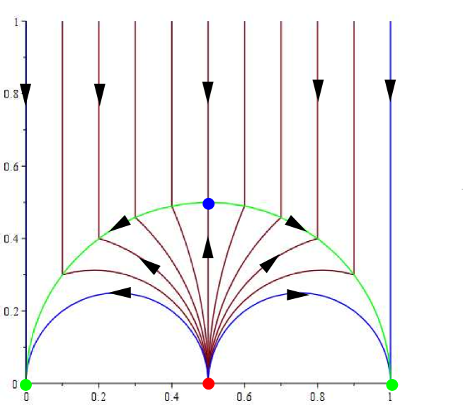
Figure 4: Temperature flow of the conductivity on the event horizon for the group $\Gamma_{0}(2)$. The fundamental domain can be taken to be the vertical strip $0\leq\sigma^{xy}\leq 1$ above the green semi-circular arc of radius one-half, spanning $0$ and $1$, the pattern repeats for $\sigma^{xy}\rightarrow\sigma^{xy}+n$ for any integer $n$. The temperature flow of the purely magnetic solution in the fundamental domain is shown together with one other copy obtained by applying the $\Gamma_{0}(2)$ transformation $\begin{pmatrix}1&-1\\ 2&-1\end{pmatrix}\in\Gamma_{0}(2)$ which leaves $\sigma_{*}=\frac{1}{2}(1+i)$ fixed.

6.2.1 Gradient flow for $\Gamma_{0}(2)$

For $\Gamma_{0}(2)$ there is a parallel theorem about modular forms to that used for $\Gamma(1)$ in §6.1, [81]: any modular form of weight -2 for $\Gamma_{0}(2)$ can be written as

$$\widetilde{\Phi}_{-2}(\sigma)=\frac{\widetilde{P}(f)}{\widetilde{Q}(f)}\frac{1}{f^{\prime}}$$

where $f(\sigma)$ is the $\Gamma_{0}(2)$ invariant function

$$f(\sigma)=-\frac{1}{256q^{2}}\prod_{n=1}^{\infty}\frac{(1-q^{4n-2})^{8}}{(1+q^{2n})^{16}},$$

with $q=e^{i\pi\sigma}$ and $\widetilde{P}(f)$ and $\widetilde{Q}(f)$ polynomials in $f$. So we can investigate $\overline{\widetilde{V}}(\bar{\sigma})=\{\overline{\widetilde{\Phi}}_{-2}\}^{-1}$ as a potential. On the vertical line in figure 4, associated with the magnetic solution with $\chi_{0}$, $\sigma=i\Theta^{4/z}$, $q=e^{-\pi\Theta^{4/z}}$ is real and hence $f$ is real on this line, it is in fact negative and runs monotonically down from $0$ to $-\infty$ as $\Theta$ increases from $0$ to $\infty$. Since $f$ is invariant under $\Gamma_{0}(2)$ transformations it is real and negative on the blue semi-circles in figure 4, which images of the imaginary axis under $\Gamma_{0}(2)$.

However $\Gamma_{0}(2)$ has another fixed point at $\sigma_{*}=\frac{1+i}{2}$, and its images, and $f=\frac{1}{4}$ at $\sigma_{*}$. Just as $J$ does for $\Gamma(1)$, $f$ takes all complex values once and only once in the fundamental domain of $\Gamma_{0}(2)$. With the same assumption as in section §6.1, that there are no fixed points of $\beta$ other than the fixed points of $\Gamma_{0}(2)$, the form of $\widetilde{P}(f)$ and $\widetilde{Q}(f)$ are then constrained so that

$$\frac{\widetilde{Q}(f)}{\widetilde{P}(f)}=\overline{C}f^{m}\left(\frac{1}{4}-f\right)^{n}$$

and

$$\beta=C\Theta^{8/z}\bar{f}^{m}\left(\bar{f}-\frac{1}{4}\right)^{n}\frac{d\bar{f}}{d\bar{\sigma}}$$

for the purely magnetic solution, with $C$ a constant. The reasoning now follows along the same lines as for $\Gamma(1)$, except the purely magnetic solution is used on the imaginary axis bounding the fundamental domain ($\chi_{0}=0$) instead of the electric one.

• $\bm{\sigma_{*,1},\sigma\rightarrow i\infty}$: for the purely magnetic solution $\sigma=i\Theta^{4/z}\rightarrow i\infty$ at large $T$ and it is known (see appendix §C) that $f\approx-\frac{e^{2\pi\Theta^{4/z}}}{256}$, $\bar{f}^{\prime}\approx 2\pi i\bar{f}$, so

  $$\beta\approx 2\pi i(-1)^{m+n+1}C\Theta^{8/z}\frac{e^{2\pi(m+n+1)\Theta^{4/z}}}{(256)^{m+n+1}}.$$

  For $\beta$ to be analytic as $\Theta\rightarrow\infty$, $n$ and $m$ must be restricted to ensure that $m+n+1<0$, but there are three fixed points in the fundamental domain and, as before, it will not be possible have $\beta$ analytic at all three so $\beta$ will not be constrained to be analytic as $T\rightarrow\infty$. The least extreme case is the marginal one, $m+n+1=0$, for which

  $$\xi\frac{d\Theta^{4/z}}{d\xi}=2\pi C\Theta^{8/z}\quad\Rightarrow\quad\xi\approx\xi_{0}\exp\left(-\frac{1}{2\pi C\Theta^{4/z}}\right)$$

  and the coherence length increase with increasing $T$ if $C>0$ tending to a constant as $\Theta\rightarrow\infty$.

• $\bm{\sigma\rightarrow 0}$: in the opposite limit, for $\Theta\rightarrow 0$, $f$ vanishes as $f\approx-16e^{-\pi/\Theta^{4/z}}$ and $\bar{f}^{\prime}\approx-\frac{16\pi i}{\Theta^{8/z}}e^{-\pi/\Theta^{4/z}}$ so

  $$\beta\approx(-1)^{m+n+1}4^{(2m-n+2)}iC\pi e^{-\pi(m+1)/\Theta^{4/z}}.$$

  Only $m=-1$ gives analytic behaviour for $\beta$ and, for $n=0$,

  $$\xi\frac{d\Theta^{4/z}}{d\xi}\approx\frac{(-1)^{n}\pi C}{4^{n}}\quad\Rightarrow\quad\xi\approx\tilde{\xi}_{0}\exp\left(\frac{(-1)^{n}2^{2n}\Theta^{4/z}}{\pi C}\right).$$

• $\bm{\sigma_{*}=\frac{1+i}{2}}$: lastly there are the new fixed points at $\sigma_{*}=\frac{1+i}{2}$ and its images. For $\sigma=\sigma_{*}+\epsilon$,

  $$f\approx\frac{1}{4}-\frac{\Gamma(1/4)^{8}}{64\pi^{4}}\epsilon^{2}$$

  and the metric contributes a factor of $\frac{1}{4}$. With $m=-1$

  $$\beta\approx(-1)^{n}2C\left\{\frac{\Gamma(1/4)^{8}}{64\pi^{4}}\right\}^{n+1}\bar{\epsilon}^{2n+1}.$$

  Analyticity requires $n\geq 0$ and $m+n+1=0$ imposes $n=0$, giving scaling behaviour

  $$\beta\approx-\frac{\Gamma(1/4)^{8}}{32\pi^{4}}C\bar{\epsilon}.$$ (90)

  In contrast to the $\Gamma(1)$ case the temperature dependence of $\bar{\epsilon}$ near $\sigma_{*}$ for $\Gamma_{0}(2)$ can be determined by going back to the full $\Gamma(1)$ configuration in §6.1 and mapping its template flow (i.e. the positive imaginary axis together with its fixed point at $\sigma_{*,2}=i$) to the semi-circle that is the lower bound of the fundamental domain of $\Gamma_{0}(2)$ in figure 4 (i.e. the semi-circular arc of radius one-half spanning the two points $\sigma=0$ and $\sigma=1$). This is achieved by using the $\Gamma(1)$ transformation $\begin{pmatrix}0&1\\ -1&\ 1\end{pmatrix}$, which is not in $\Gamma_{0}(2)$, and sends $\sigma_{*,2}$ to $\sigma_{*}=\frac{1+i}{2}$. The semi-circle can then be mapped around the upper half-plane using $\Gamma_{0}(2)$.

  To apply equation (90) in this topology observe that $\begin{pmatrix}0&1\\ -1&\ 1\end{pmatrix}$ sends

  $$i\Theta^{4/z}\rightarrow\frac{1+i\Theta^{4/z}}{1+\Theta^{8/z}}\qquad\mbox{and}\qquad i\Theta^{-4/z}\rightarrow\frac{1+i\Theta^{-4/z}}{1+\Theta^{-8/z}}$$

  with $0\leq\Theta\leq 1$. Near the critical point $\sigma_{*,2}=i$, where $\Theta=1-{\tt t}$, the image is

  $$\left(\frac{1+i}{2}\right)\pm\frac{2{\tt t}}{z}$$

  with positive ${\tt t}$ just below $\sigma_{*,2}$ in the $\Gamma(1)$ template mapped to the right-hand half of the semi-circle ($+$ sign) and positive ${\tt t}$ just above $\sigma_{*,2}$ mapped to the left-hand half ($-$ sign), with $\bar{\epsilon}=\pm\frac{2{\tt t}}{z}$ when ${\tt t}$ is small. In either case the sign in (90) makes $\frac{1+i}{2}$ a repulsive fixed point if $C$ is positive and

  $$\xi\sim{\tt t}^{-\nu^{\prime}}$$

  with critical exponent

  $$\nu^{\prime}=\frac{32\pi^{4}}{C\{\Gamma(1/4)\}^{8}}.$$

In summary the $\Gamma_{0}(2)$ flow with $m=-1$ and $n=0$ has $\beta$-function

$$\beta=C\{Im(\sigma)\}^{2}\frac{d\ln|\bar{f}|}{d\bar{\sigma}}$$ (91)

with $C>0$ and the fixed point behaviour of the coherence length is

$$\xi\sim\begin{cases}\xi_{0}\exp\left(-\frac{1}{2\pi C\Theta^{4/z}}\right),&\Theta\rightarrow\infty,\ \sigma\rightarrow i\infty;\\ \tilde{\xi}_{0}\exp\left(\frac{\Theta^{4/z}}{\pi C}\right),&\Theta\rightarrow 0,\ \sigma\rightarrow 0;\\ A{\tt t}^{-\nu\,^{\prime}},&\Theta\rightarrow 1,\ \sigma\rightarrow\frac{1+i}{2},\ \mbox{with}\ \nu^{\prime}=\frac{32\pi^{4}}{C\bigl{\{}\Gamma(\frac{1}{4})\bigr{\}}^{8}}.\end{cases}$$ (92)

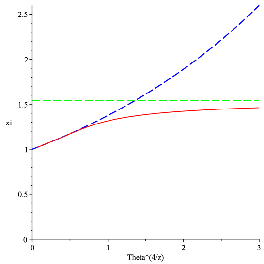
Figure 5: $\xi$ along the imaginary axis $\sigma=i\Theta^{4/z}$ for the purely magnetic solution as a function of $\Theta^{4/z}$. $\Gamma_{0}(2)$ symmetry determines the behaviour near $\Theta=0$, via (92), and (91) is numerically integrated to determine $\xi\bigl{(}\Theta^{4/z}\bigr{)}$. The red curve is the numerical result for the specific choice $\tilde{\xi}_{0}=C=1$. The dashed blue curve is the asymptotic form $\xi=e^{\Theta^{4/z}/\pi}$ near $\Theta=0$ and the dashed green curve is the asymptotic value for $\tilde{\xi}_{0}=C=1$, which numerically is $\xi_{0}\approx 1.540$. Again this assumes that the classical solution gives the correct temperature dependence along the imaginary axis.

Extending the temperature into the whole fundamental domain by assuming that $\Theta(f,\bar{f})$ is a real modular invariant function that increases monotonically as $|f|$ increases the flow can be obtained by plotting lines of constant $\arg(f)$ in the conductivity plane. The result is shown in figure 6 which is taken from the review [84] and has the same topology as the $\Gamma_{0}(2)$ flow originally suggested in [85, 86]. Flow lines in the conductivity plane, in terms of electron coherence length, were suggested for the integer QHE in [87] and the hierarchical structure of modular symmetry extends this to the fractional effect.

Note that it is not being assumed that $\Theta$ is independent of $\arg(f)$, only that the temperature flow is obtained by varying $|f|$, keeping $\arg(f)$ fixed. For $\sigma=i\Theta^{4/z}$, $f$ is real and negative, so $\arg(f)=\pi$, while on the semi-circle passing through $\sigma_{*}$, $f$ is real and positive, so $\arg(f)=0$. The anti-holomorphic $\beta$-function in (91) was first proposed in [36, 37, 38].

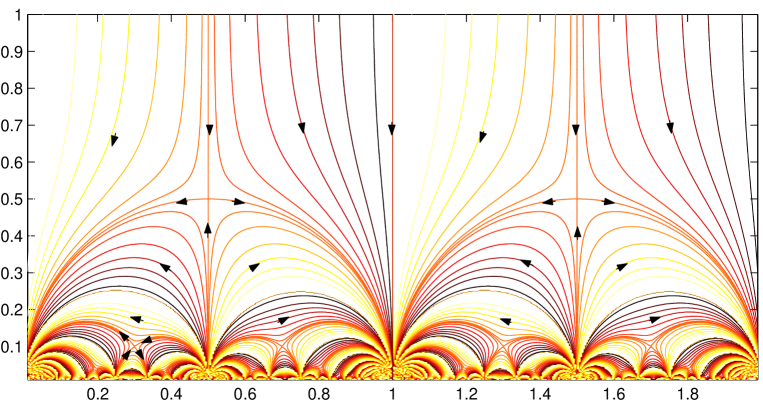
Figure 6: Temperature flow of the conductivity on the event horizon for $\Gamma_{0}(2)$ symmetry, assuming it is generated by varying $|f|$, keeping $\arg(f)$ fixed. The diagram is obtained simply by plotting lines of constant $\arg(f)$ as in [39].

Figure 6 should be compared to the experimental plots in [42] and [43] (similar experimental plots have been obtained by other groups [44]). The agreement is remarkable.

7 Discussion

There are two distinct aspects to the discussion presented here: the AdS/CMT paradigm and gradient flow. They are woven together in the analysis but are a priori independent concepts.

The idea of gradient flow $\beta$-functions for the QHE is motivated by the $c$-theorem in 2-dimensions and was first used in the context of modular symmetry more than 20 years ago [34, 35]. In that work the function $f^{\prime}/f$ was considered but rejected it because it did not match perturbation theory for large values of the Ohmic conductivity. In the context of the AdS/CMT correspondence that is not a reason to reject it as the perturbative limit of the boundary theory is not accessible from the classical bulk theory, analysing the perturbative limit would require understanding quantum gravity effects in the bulk.

As mentioned in the introduction a number of authors have considered describing the QHE within the framework of AdS/CMT, including in particular [10] where the Gibbons-Rasheed action was used near the horizon to analyse the conductivity associated with a dyonic solution in the bulk and [33] where the Dirac quantisation condition in the bulk was used to argue for fractional filling factors. The new ingredients here are the observation that the infra-red DC conductivity at $u\rightarrow 1$ is identified with the value of the dilaxion on the horizon and that this is consistent with gradient flow.

The assumption that $\Theta$ is a monotonic function of $|f|$ and that the flow lines are given by varying $|f|$ keeping $\arg(f)$ fixed needs some discussion (we shall discuss $\Gamma_{0}(2)$ here, as that is more relevant to experiment, a similar discussion can be given for $\Gamma(1)$ with $f$ replaced by $J$). $\Theta$ is a monotonic function of $|f|$ on the positive imaginary axis, where $\arg(f)=\pi$, and extending this into the interior of the fundamental domain requires turning on a non-zero $\chi_{0}$ and changing $\arg(f)$, so that $\arg(f)$ is correlated in some way with $\chi_{0}$ in the classical solution. Experimentally [42]-[44] this can be achieved in the QHE by varying the magnetic field away from its critical value $B_{*}$. In the composite fermion picture $B_{*}$ corresponds to the situation when the statistical gauge field exactly cancels the applied field, the 2DEG is a composite fermi liquid [33]. In our scenario $B_{*}$ corresponds to $\lambda\chi_{0}=1/2$ and deviations from $B_{*}$ arise not from varying the dyon magnetic charge, which relates to a global $U(1)$ on the boundary, but from varying $\chi_{0}$ (in [33] $\chi_{0}$ is set to zero). Exactly how $\chi_{0}$ might be related to the deviation of the external field from its critical value would depend on the details of the underlying matter and an investigation of this would require numerical analysis of an underlying fermionic matter action. But the basic idea that varying $T$ and $B$ independently is equivalent to varying $\zeta$ and $\chi_{0}$, or $|f|$ and $\arg(f)$, is not obviously inconsistent and seems at least plausible.

Lastly we comment on possible sub-groups of $\Gamma(1)$. Two scenarios have been presented involving $\Gamma(1)$ and $\Gamma_{0}(2)$ flow with very different topologies, but there are other possibilities. For example $\Gamma(2)$, generated by ${\bm{S}}{\bm{T}}^{2}{\bm{S}}$ and ${\bm{T}}^{2}$, was studied in [88] in the context of the QHE and is relevant for spin-degenerate quantum Hall systems [89]. Another level 2 sub-group, $\Gamma_{\theta}$ (see appendix C), was suggested as being relevant for bosonic charge carriers in a superconductor in a magnetic field in [11]. The possibility of ${\bf T}$ versus ${\bf T}^{2}$ was discussed in [83] where it was related to whether or not the Euclidean version of the bulk theory is formulated on a 4-manifold admitting a spin structure. There is nothing in the classical solutions presented here that picks out any preferred level 2 sub-group associated with any particular kind of matter, the dilaton is not charged and merely plays the rôle of an effective background electric susceptibility after any matter fields have been integrated out. Presumably a more detailed bulk model, included matter, is needed to pick out a specific level 2 sub-group. For example fermionic matter in the bulk would be expected to give $\Gamma_{0}(2)$ and bosonic matter $\Gamma_{\theta}$. The full group $\Gamma(1)$ might require supersymmetric matter, though a phase diagram with $\Gamma(1)$ symmetry was proposed for a 2-dimensional Abelian lattice model in [90] (to the author’s knowledge this was actually the first suggestion of $Sl(2,{\bm{Z}})$ duality transformations between different phases) but this is left as a subject for future investigation.

Appendix A Conventions

The conventions used in the text for the computation of the conductivity in appendix B are collected here for convenient reference.

Our signature is $(-,+,+,+)$ with line element

$$ds=\frac{1}{u^{2}}\left(-f^{2}d\tilde{t}\,^{2}+\frac{l^{2}}{h^{2}}du^{2}+dx^{2}+dy^{2}\right),$$ (93)

where $u=\frac{r_{h}}{r}$ and $f$ has a single zero at $u=1$, with asymptotic infinity at $u\rightarrow 0$. The magnetic field tensor $F_{\mu\nu}$ decomposes into electric and magnetic fields as

$$E_{\alpha}=-F_{\tilde{t}{\alpha}},\qquad B^{\alpha}=-\widetilde{F}^{\tilde{t}{\alpha}}=-\frac{1}{2}\frac{\epsilon^{\tilde{t}{\alpha}{\beta}{\gamma}}}{\sqrt{-g}}F_{{\beta}{\gamma}}$$

with ${\alpha},{\beta},{\gamma}=u,x,y$ and $\epsilon_{\tilde{t}uxy}=-\epsilon^{\tilde{t}uxy}=1$. Under a perturbations homogeneous in the transverse directions, the transverse field variations are

$$\delta E_{\alpha}=-\delta F_{\tilde{t}{\alpha}},\qquad\delta B^{\alpha}=-\delta\widetilde{F}^{\tilde{t}{\alpha}}=-\frac{u^{4}h}{lf}\epsilon^{{\alpha}{\beta}}(\delta F_{u{\beta}})=-\frac{u^{4}h}{lf}\epsilon^{{\alpha}{\beta}}(\delta A_{\beta}^{\prime})$$

with $\epsilon^{xy}=-\epsilon^{yx}=1$ and ${\alpha},{\beta}$ restricted to $x,y$.

Conductivities are calculated in a local inertial frame and we need these expressions in an orthonormal basis. With transverse orthonormal indices $i,j=2,3$ the orthonormal components of ${\bf E}$ and ${\bf B}$ are

$$\delta E_{i}=\frac{u^{2}}{f}\delta_{i}{}^{\alpha}(\delta E_{\alpha}-\widehat{m}\epsilon_{\alpha}{}^{\beta}\delta G_{\beta}),\qquad\delta B^{i}=\frac{f}{u^{2}}\delta^{i}_{\alpha}(\delta B^{\alpha})=-\frac{u^{2}h}{l}\epsilon^{{\alpha}{\beta}}(\delta A_{\beta}^{\prime}),$$

where the metric variation is $\delta g_{\tilde{t}{\alpha}}=\frac{1}{u^{2}}\delta G_{\alpha}$ and $\widehat{m}$ is related to the magnetic charge $m$ in equation (31) by $\widehat{m}=\bigl{(}\frac{l}{r_{h}}\bigr{)}^{2}m$. It is convenient to combine these into the complex fields

$${\delta\cal E}_{\pm}=\frac{f}{u^{2}}(\delta E_{2}\pm i\delta E_{3}),\qquad{\delta\cal B}_{\pm}=\frac{f}{u^{2}}(\delta B_{2}\pm i\delta B_{3})=\frac{f^{2}}{u^{4}}(\delta B^{x}\pm i\delta B^{y}).$$

The Hodge star used in (5) is

$$*1=\sqrt{-g}\,d^{4}x=\frac{l}{u^{z+3}}(d\tilde{t}\wedge du\wedge dx\wedge dy),$$

thus $*G=\frac{\sqrt{-g}}{2}\epsilon_{\mu\nu\rho\sigma}G^{\mu\nu}dx^{\rho}\wedge dx^{\sigma}=\frac{1}{2}{\widetilde{G}}_{\rho\sigma}dx^{\rho}\wedge dx^{\sigma}$.

Appendix B Conductivities in linear response theory

Conductivities in the boundary theory can be determined using the techniques in [56] and [55]. The idea is to make a perturbation of the fields that is independent of the transverse co-ordinates $x$ and $y$ and demand that this is a solution of the bulk equations of motion at second order in the perturbation. This generates differential equations that the perturbations must satisfy which can be used to determine response functions for the boundary theory, in particular the conductivities.

Let

$$\delta g_{\tilde{t}x}=\frac{\delta G_{x}(\tilde{t},u)}{u^{2}}\qquad\delta g_{\tilde{t}y}=\frac{\delta G_{y}(\tilde{t},u)}{u^{2}}$$

be perturbations of the bulk metric

$$ds^{2}=\frac{1}{u^{2}}\left(-f^{2}(u)d\tilde{t}\,^{2}+\frac{l^{2}du^{2}}{h^{2}(u)}+dx^{2}+dy^{2}\right).$$

These are not general perturbations but are chosen to be independent of $x$ and $y$ so they are homogeneous in the transverse directions, which is sufficient for our needs. We shall also assume oscillatory time dependence and set

$$G_{x}(\tilde{t},u)=e^{-i\widetilde{\omega}\tilde{t}}\delta\widetilde{G}_{x}(u),\qquad G_{y}(\tilde{t},u)=e^{-i\widetilde{\omega}\tilde{t}}\delta\widetilde{G}_{y}(u).$$

For the explicit dyon solution in §3.2 the functions $f(u)$ and $h(u)$ are

$$f^{2}(u)=\frac{(1-u^{z+2})}{u^{2(z-1)}},\qquad h^{2}(u)=1-u^{z+2}$$

but the analysis will be kept more general and these explicit forms only used at the end. Perturbations of the dilaton and axion fields take a similar form

$$\delta\phi(\tilde{t},u)=e^{-i\widetilde{\omega}\tilde{t}}\delta\tilde{\phi}(u),\qquad\delta\chi(\tilde{t},u)=e^{-i\widetilde{\omega}\tilde{t}}\delta\tilde{\chi}(u),$$ (94)

though demanding that the perturbations satisfy the linearised equations of motion forces $\delta\tilde{\phi}(u)=\delta\tilde{\chi}(u)=0$ at this order.

A similar perturbation of a dyonic configuration, with Maxwell 2-form

$$F=dA=\frac{\widehat{q}\,lf(u)}{u^{4}h(u)}d\tilde{t}\wedge du+\widehat{m}dx\wedge dy,$$

is

$$\delta A=\delta A_{\alpha}(\tilde{t},u)dx^{\alpha}=e^{-i\widetilde{\omega}\tilde{t}}\Bigl{(}\delta\widetilde{A}_{x}(u)dx+\delta\widetilde{A}_{y}(u)dy\Bigr{)}.$$ (95)

This generates a transverse electric field

$$\delta E_{\alpha}=-\delta F_{\tilde{t}{\alpha}}=i\widetilde{\omega}\delta A_{\alpha}$$ (96)

and a transverse magnetic field

$$\delta B^{\alpha}=\frac{\epsilon^{\tilde{t}u{\alpha}{\beta}}}{\sqrt{-g}}\delta F_{u{\beta}}=-\frac{u^{4}h}{lf}\epsilon^{{\alpha}{\beta}}\delta A^{\prime}_{\beta},$$ (97)

where where ${\alpha}$ and ${\beta}$ label $x$ and $y$, $\epsilon^{\tilde{t}uxy}=-1$, $\epsilon^{xy}=+1$ and ^′ denotes differentiation with respect to $u$. For static fields

$$\delta A_{\alpha}(\tilde{t},u)=(\delta E_{\alpha}^{0})\tilde{t}+\delta\widetilde{A}_{\alpha}(u)$$ (98)

with $\delta E^{0}_{\alpha}$ constants.

In an orthonormal basis the electric and magnetic field variations are

$$\delta E_{2}=\frac{u^{2}}{f}(\delta E_{x}-\widehat{m}\delta G_{y}),\qquad\delta E_{3} = \frac{u^{2}}{f}(\delta E_{y}+\widehat{m}\delta G_{x}),$$ (99)

$$\delta B^{2}=-\frac{u^{2}h}{l}\delta A_{y}^{\prime}=\frac{f}{u^{2}}\delta B^{x},\qquad\delta B^{3} = \frac{u^{2}h}{l}\delta A_{x}^{\prime}=\frac{f}{u^{2}}\delta B^{y}.$$ (100)

These perturbations will induce a transverse current

$$\delta J^{i}=\sigma^{ij}\delta E_{j}$$

with $\sigma^{ij}$ the transverse conductivity tensor ($i,j=2.3$ are orthonormal indices). In a co-ordinate basis

$$\begin{pmatrix}\delta J^{x}\\ \delta J^{y}\end{pmatrix}=u\begin{pmatrix}\delta J^{2}\\ \delta J^{3}\end{pmatrix},\qquad\begin{pmatrix}\sigma^{xx}&\sigma^{xy}\\ \sigma^{yx}&\sigma^{yy}\end{pmatrix}=u^{2}\begin{pmatrix}\sigma^{22}&\sigma^{23}\\ \sigma^{32}&\sigma^{33}\end{pmatrix}$$

and

$$\delta J^{\alpha}=\sigma^{{\alpha}{\beta}}{\delta\cal E}_{\beta}$$

where

$${\delta\cal E}_{\alpha}=\delta E_{\alpha}-\widehat{m}\epsilon_{\alpha}{}^{\beta}\delta G_{\beta}.$$ (101)

With the complex combinations

$${\delta\cal E}_{\pm}={\delta\cal E}_{x}\pm i{\delta\cal E}_{y},\qquad\delta J_{\pm}=\delta J^{x}\pm i\delta J^{y},\qquad\sigma_{\pm}=\sigma^{xy}\pm i\sigma^{xx}$$ (102)

this is [55]

$$\sigma_{\pm}=\pm i\frac{\delta J_{\pm}}{{\delta\cal E}_{\pm}}.$$ (103)

In AdS/CMT correlations functions are derived from the boundary action. With any fixed value of $\delta A_{\alpha}|_{u=1}$ at the event horizon we can cut the bulk theory off at a finite value of $u<1$ to find that the variation of the action is

$$\delta S[\delta A(u),\delta G(u)] =\int d\tilde{t}\,dx\,dy\left[\delta A_{\alpha}\left(-\frac{1}{2}e^{-\lambda\phi}\delta F^{u{\alpha}}\sqrt{-g}+\frac{\lambda\chi}{2}\epsilon^{u{\alpha}\tilde{t}{\beta}}\delta F_{\tilde{t}{\beta}}\right)\right]_{u}^{1}$$

$$=\frac{1}{2}\int d\tilde{t}\,dx\,dy\left.\Bigl{\{}\delta A_{\alpha}\left(e^{-\lambda\phi}\delta F^{u{\alpha}}\sqrt{-g}-\lambda\chi\epsilon^{u{\alpha}\tilde{t}{\beta}}\delta F_{\tilde{t}{\beta}}\right)\Bigr{\}}\right|_{u}+const.$$

(the Einstein action gives no contribution at $O(\delta G_{\alpha}^{2})$ ). The current is then

$$\delta J^{\alpha}(u) =\frac{\delta S}{\delta A_{\alpha}}=e^{-\lambda\phi}\delta F^{u{\alpha}}\sqrt{-g}-\lambda\chi\epsilon^{\tilde{t}u{\alpha}{\beta}}\delta F_{\tilde{t}{\beta}}$$ (104)

$$=\frac{e^{-\lambda\phi}}{u^{4}}\delta^{{\alpha}{\beta}}\left\{f^{2}\epsilon_{{\beta}{\gamma}}(\delta B^{\gamma})-\widehat{q}\,(\delta G_{\beta})\right\}-\lambda\chi\epsilon^{{\alpha}{\beta}}(\delta E_{\beta})$$ (105)

where we have used

$$\delta F^{u{\alpha}}=\delta^{{\alpha}{\beta}}\left(\frac{u^{4}h^{4}}{l^{2}}\delta A_{\beta}-\frac{\widehat{q}\,h}{lf}\delta G_{\alpha}\right),\qquad\sqrt{-g}=\frac{lf}{u^{4}h},$$

and (97). This can be re-expressed as

$$\delta J^{\alpha}=e^{-\lambda\phi}\delta^{{\alpha}{\beta}}\epsilon_{{\beta}{\gamma}}({\delta\cal B}^{\gamma})-\lambda\chi\epsilon^{{\alpha}{\beta}}{\delta\cal E}_{\beta}+\delta^{{\alpha}{\beta}}\left(\lambda\widehat{m}\chi-\frac{\widehat{q}e^{-\lambda\phi}}{u^{4}}\right)\delta G_{\beta}$$

where, following [55], we define

$${\delta\cal B}^{\alpha}=\frac{f^{2}}{u^{4}}\delta B^{\alpha}=\frac{f}{u^{2}}\delta^{\alpha}_{i}(\delta B^{i})$$

in analogy with

$${\delta\cal E}_{\alpha}=\frac{f}{u^{2}}\delta_{\alpha}^{i}(\delta E_{i}).$$

From these the transverse conductivity, ignoring the back-reaction on the metric, is

$$\sigma^{{\alpha}{\beta}}=\left.\frac{\delta J^{\alpha}}{{\delta\cal E}_{\beta}}\right|_{\delta G_{\pm}=0}=e^{-\lambda\phi}\left(\frac{\epsilon^{\alpha}{}_{\gamma}{\delta\cal B}^{\gamma}}{{\delta\cal E}_{\beta}}\right)-\lambda\chi\epsilon^{{\alpha}{\beta}}$$ (106)

or

$$\sigma_{\pm}=e^{-\lambda\phi}\frac{{\delta\cal B}_{\pm}}{{\delta\cal E}_{\pm}}-\lambda\chi,$$ (107)

which is central to the analysis in the text.

We note in passing that

$$\left.\frac{\delta J^{\alpha}}{\delta G_{\beta}}\right|_{{\delta\cal E}_{\pm}=0}=\left(\lambda\widehat{m}\chi-\frac{\widehat{q}e^{-\lambda\phi}}{u^{4}}\right)\delta^{{\alpha}{\beta}}=\frac{\widehat{m}{a}}{{c}}\delta^{{\alpha}{\beta}}=\frac{Q_{e}}{{\cal A}_{h}}\delta^{{\alpha}{\beta}},$$ (108)

where the final two equalities are specifically for the dyon solution (30) with electric charge (36). $\frac{Q_{e}}{{\cal A}_{h}}$ is of course the charge density at the event horizon and $u^{2}\frac{\delta J^{\alpha}}{\delta G_{\beta}}=<J^{\alpha}T^{\tilde{t}{\beta}}>$ is piezoelectric tensor for the deformation $\delta g_{\tilde{t}{\beta}}$.

B.1 RG equation for the conductivities

To obtain more detailed information about the conductivity we need a relation between ${\delta\cal B}^{\alpha}$ and ${\delta\cal E}_{\alpha}$ and this comes from requiring that these variations are solutions of the linearised equations of motion. These are Einstein’s equations

$$\frac{fh}{4\kappa^{2}l^{2}}\left(\frac{h}{f}\frac{\delta G_{x}^{\prime}}{u^{2}}\right)^{\prime}+e^{-\lambda\phi}\left(-\frac{fh}{l}\frac{\widehat{q}}{u^{4}}\delta A_{x}^{\prime}-\widehat{m}(i\widetilde{\omega}\delta A_{y}+\widehat{m}\delta G_{x})\right) = 0,$$ (109)

$$\frac{fh}{4\kappa^{2}l^{2}}\left(\frac{h}{f}\frac{\delta G_{y}^{\prime}}{u^{2}}\right)^{\prime}+e^{-\lambda\phi}\left(-\frac{fh}{l}\frac{\widehat{q}}{u^{4}}\delta A_{y}^{\prime}+\widehat{m}(i\widetilde{\omega}\delta A_{x}-\widehat{m}\delta G_{y})\right) = 0,$$ (110)

$$\frac{i\widetilde{\omega}}{4\kappa^{2}}\left(\frac{\delta G_{x}^{\prime}}{u^{2}}\right)+e^{-\lambda\phi}\left(-\frac{lf}{h}\frac{\widehat{q}}{u^{4}}(i\widetilde{\omega}\delta A_{x}-\widehat{m}\delta G_{y})-\widehat{m}f^{2}\delta A_{y}^{\prime}\right) = 0,$$ (111)

$$\frac{i\widetilde{\omega}}{4\kappa^{2}}\left(\frac{\delta G_{y}^{\prime}}{u^{2}}\right)+e^{-\lambda\phi}\left(-\frac{lf}{h}\frac{\widehat{q}}{u^{4}}(i\widetilde{\omega}\delta A_{y}+\widehat{m}\delta G_{x})+\widehat{m}f^{2}\delta A_{x}^{\prime}\right) = 0,$$ (112)

and Maxwell’s equation

$$\partial_{\mu}\bigl{(}\sqrt{-g}\,e^{-\lambda\phi}\delta F^{\mu\nu}\bigr{)}-\frac{\lambda}{2}\epsilon^{\mu\nu\sigma\lambda}(\partial_{\mu}\chi)\delta F_{\sigma\lambda}=0\qquad\Rightarrow$$

$$-\frac{i\widetilde{\omega}l}{fh}e^{-\lambda\phi}\bigl{(}i\widetilde{\omega}\delta A_{\alpha}-\widehat{m}\epsilon_{\alpha}{}^{\beta}\delta G_{\beta}\bigr{)}+\left(\frac{fh}{l}e^{-\lambda\phi}(\delta A_{\alpha})^{\prime}-\frac{\widehat{q}}{u^{4}}\delta G_{\alpha}\right)^{\prime} =i\widetilde{\omega}\lambda\chi^{\prime}\epsilon_{{\alpha}}^{\beta}\delta A_{\beta},$$ (113)

while the dilaton and axion equations of motion impose

$$\delta\phi=\delta\chi=0$$ (114)

(see [56], the only new ingredient here is the dilaton and axion for which a perturbation of the form (94) is constrained to vanish by the equations of motion).

In terms of

$${\delta\cal E}_{x} = i\widetilde{\omega}\delta A_{x}-\widehat{m}\delta G_{y},$$ (115)

$${\delta\cal E}_{y} = i\widetilde{\omega}\delta A_{y}+\widehat{m}\delta G_{x},$$ (116)

$${\delta\cal B}^{x} = -\frac{fh}{l}\delta A_{y}^{\prime},$$ (117)

$${\delta\cal B}^{y} = \frac{fh}{l}\delta A_{x}^{\prime},$$ (118)

equations (109)-(112) can be re-cast as

$$\frac{fh}{4\hat{\kappa}^{2}}\left(\frac{h}{f}\frac{\delta G_{x}^{\prime}}{u^{2}}\right)^{\prime} = e^{-\lambda\phi}\left(\widehat{m}{\delta\cal E}_{y}+\frac{\widehat{q}}{u^{4}}{\delta\cal B}^{y}\right),$$ (119)

$$\frac{fh}{4\hat{\kappa}^{2}}\left(\frac{h}{f}\frac{\delta G_{y}^{\prime}}{u^{2}}\right)^{\prime} = e^{-\lambda\phi}\left(-\widehat{m}{\delta\cal E}_{x}-\frac{\widehat{q}}{u^{4}}{\delta\cal B}^{x}\right),$$ (120)

$$\frac{i\widehat{\omega}}{4\hat{\kappa}^{2}}\frac{h}{f}\left(\frac{\delta G_{x}^{\prime}}{u^{2}}\right) = e^{-\lambda\phi}\left(\frac{\widehat{q}}{u^{4}}{\delta\cal E}_{x}-\widehat{m}{\delta\cal B}^{x}\right),$$ (121)

$$\frac{i\widehat{\omega}}{4\hat{\kappa}^{2}}\frac{h}{f}\left(\frac{\delta G_{y}^{\prime}}{u^{2}}\right) = e^{-\lambda\phi}\left(\frac{\widehat{q}}{u^{4}}{\delta\cal E}_{y}-\widehat{m}{\delta\cal B}^{y}\right),$$ (122)

with $\hat{\kappa}=\kappa l$ and $\widehat{\omega}=\widetilde{\omega}l$ while (113) is

$$-\frac{i\widehat{\omega}}{fh}e^{-\lambda\phi}({\delta\cal E}_{\pm})+\bigl{(}\epsilon_{\alpha}{}^{\beta}{\delta\cal B}_{\beta}-\frac{\widehat{q}}{u^{4}}\delta G_{\alpha}\bigr{)}^{\prime}=i\widehat{\omega}\lambda\chi^{\prime}\epsilon_{{\alpha}}^{\beta}({\delta\cal E}_{\beta}+\widehat{m}\epsilon_{\beta}{}^{\gamma}\delta G_{\beta}).$$

Now differentiate (121) and (122) and equate the result to (119) and (120) giving

$$\left\{e^{-\lambda\phi}\left(-\frac{\widehat{q}}{u^{4}}{\delta\cal E}_{\pm}+\widehat{m}{\delta\cal B}_{\pm}\right)\right\}^{\prime}=\mp\frac{\widehat{\omega}e^{-\lambda\phi}}{fh}\left(\widehat{m}{\delta\cal E}_{\pm}+\frac{\widehat{q}}{u^{4}}{\delta\cal B}_{\pm}\right).$$ (123)

A second equation relating ${\delta\cal E}_{\pm}^{\prime}$ to ${\delta\cal E}_{\pm}$ and ${\delta\cal B}_{\pm}$ is obtained from (115) and (116),

$$\delta G_{x}=\frac{1}{\widehat{m}}(-i\widetilde{\omega}\delta A_{y}+{\delta\cal E}_{y}),\qquad\delta G_{y}=\frac{1}{\widehat{m}}(i\widetilde{\omega}\delta A_{x}-{\delta\cal E}_{x}),$$ (124)

from which

$$\delta G_{x}^{\prime}=\frac{1}{\widehat{m}}\left(\frac{i\widehat{\omega}}{fh}{\delta\cal B}^{x}+{\delta\cal E}_{y}^{\prime}\right),\qquad\delta G_{y}^{\prime}=\frac{1}{\widehat{m}}\left(\frac{i\widehat{\omega}}{fh}{\delta\cal B}^{y}-{\delta\cal E}_{x}^{\prime}\right).$$ (125)

Now using these to eliminate $\delta G_{\alpha}^{\prime}$ in (121) and (122) leads to

$$\frac{\widehat{\omega}}{4\hat{\kappa}^{2}u^{2}}\left(\mp{\delta\cal E}_{\pm}^{\prime}+\frac{\widehat{\omega}}{fh}{\delta\cal B}_{\pm}\right)=e^{-\lambda\phi}\frac{f}{h}\left(-\frac{\widehat{q}\widehat{m}}{u^{4}}{\delta\cal E}_{\pm}+\widehat{m}^{2}{\delta\cal B}_{\pm}\right).$$ (126)

Equations (123) and (126) here are the analogues of equations (17) and (18) in [55].

It is convenient to define

$${\cal Q}=\frac{e^{-\lambda\phi}\widehat{q}}{u^{4}},\qquad{\cal M}=e^{-\lambda\phi}\widehat{m},\qquad\delta{\cal G}_{\pm}=\delta{\cal G}_{x}\pm i\delta{\cal G}_{y},$$ (127)

in terms of which (123), (125) and (126) can be written as a matrix equation

$$\begin{pmatrix}-{\cal Q}&{\cal M}&0\\ \mp\frac{\widehat{\omega}}{4\hat{\kappa}^{2}u^{2}}&0&0\\ 1&0&\mp i\widehat{m}\end{pmatrix}\begin{pmatrix}{\delta\cal E}^{\prime}_{\pm}\\ {\delta\cal B}^{\prime}_{\pm}\\ \delta{\cal G}^{\prime}_{\pm}\end{pmatrix} =\begin{pmatrix}{\cal Q}^{\prime}\mp\frac{\widehat{\omega}}{fh}{\cal M}&-{\cal M}^{\prime}\mp\frac{\widehat{\omega}}{fh}{\cal Q}&0\\ -\frac{f\widehat{m}}{h}{\cal Q}&\frac{f\widehat{m}}{h}{\cal M}-\frac{\widehat{\omega}^{2}}{4\hat{\kappa}^{2}u^{2}fh}&0\\ -\frac{4i\hat{\kappa}^{2}u^{2}f}{\widehat{\omega}h}{\cal Q}&\frac{4i\hat{\kappa}^{2}u^{2}f}{\widehat{\omega}h}{\cal M}&0\end{pmatrix}\begin{pmatrix}{\delta\cal E}_{\pm}\\ {\delta\cal B}_{\pm}\\ \delta{\cal G}_{\pm}\end{pmatrix}$$

$$\Rightarrow\qquad\begin{pmatrix}{\delta\cal E}^{\prime}_{\pm}\\ {\delta\cal B}^{\prime}_{\pm}\\ \delta{\cal G}^{\prime}_{\pm}\end{pmatrix} =\begin{pmatrix}{\cal S}_{11}&{\cal S}_{12}&0\\ {\cal S}_{21}&{\cal S}_{22}&0\\ {\cal S}_{31}&{\cal S}_{32}&0\end{pmatrix}\begin{pmatrix}{\delta\cal E}_{\pm}\\ {\delta\cal B}_{\pm}\\ \delta{\cal G}_{\pm}\end{pmatrix}$$ (128)

with

$${\cal S}_{11} =\pm\frac{4\hat{\kappa}^{2}u^{2}}{\widehat{\omega}}\frac{f\widehat{m}}{h}{\cal Q}$$

$${\cal S}_{12} =\mp\frac{4\hat{\kappa}^{2}u^{2}}{\widehat{\omega}}\frac{f\widehat{m}}{h}{\cal M}\pm\frac{\widehat{\omega}}{fh}$$

$${\cal S}_{21} =\pm\frac{4\hat{\kappa}^{2}u^{2}}{\widehat{\omega}}\frac{f\widehat{m}}{h}\frac{{\cal Q}^{2}}{{\cal M}}+\frac{{\cal Q}^{\prime}}{{\cal M}}\mp\frac{\widehat{\omega}}{fh}$$

$${\cal S}_{22} =\mp\frac{4\hat{\kappa}^{2}u^{2}}{\widehat{\omega}}\frac{f\widehat{m}}{h}{\cal Q}-\frac{{\cal M}^{\prime}}{{\cal M}}$$ (129)

$${\cal S}_{31} =-\frac{4i\hat{\kappa}^{2}u^{2}f}{\widehat{\omega}h}{\cal Q}$$

$${\cal S}_{32} =\frac{4i\hat{\kappa}^{2}u^{2}f}{\widehat{\omega}h}{\cal M}.$$

From these we get

$$\left(\frac{{\delta\cal B}_{\pm}}{{\delta\cal E}_{\pm}}\right)^{\prime} =$$ (130)

$$\kern-50.0pt\pm\frac{4\hat{\kappa}^{2}u^{2}}{\widehat{\omega}}\frac{f}{h}\frac{\widehat{m}}{{\cal M}}\left\{-{\cal Q}+{\cal M}\left(\frac{{\delta\cal B}_{\pm}}{{\delta\cal E}_{\pm}}\right)\right\}^{2}\mp\frac{\widehat{\omega}}{fh}\left\{1+\left(\frac{{\delta\cal B}_{\pm}}{{\delta\cal E}_{\pm}}\right)^{2}\right\}-\frac{{\cal M}^{\prime}}{{\cal M}}\left(\frac{{\delta\cal B}_{\pm}}{{\delta\cal E}_{\pm}}\right)+\frac{{\cal Q}^{\prime}}{{\cal M}}.$$

A renormalisation group equation for the conductivity tensor follows from this [57]. Again with

$$\Sigma_{\pm}=e^{-\lambda\phi}\frac{\delta{\cal B}_{\pm}}{\delta{\cal E}_{\pm}}$$

using (127) gives

$$\left(\Sigma_{\pm}-\frac{\widehat{q}e^{-\lambda\phi}}{\widehat{m}u^{4}}\right)^{\prime}=\pm\frac{4\hat{\kappa}^{2}u^{2}}{\widehat{\omega}}\frac{f}{h}\left(\widehat{m}\Sigma_{\pm}-\frac{\widehat{q}e^{-\lambda\phi}}{u^{4}}\right)^{2}\mp\frac{\widehat{\omega}e^{-\lambda\phi}}{fh}\left(1+e^{2\lambda\phi}\Sigma_{\pm}^{2}\right)$$

Putting the dyon solution

$$f(u)=\frac{\sqrt{1-u^{z+2}}}{u^{z-1}},\qquad h(u)=\sqrt{1-u^{z+2}},\qquad e^{-\lambda\phi}=\frac{u^{4}}{{d}^{2}+{c}^{2}\zeta^{2}u^{8}}$$

into this results in

$$\pm\frac{\widehat{\omega}}{\widehat{m}}\left(\widehat{m}\Sigma_{\pm}-\frac{\widehat{q}e^{-\lambda\phi}}{u^{4}}\right)^{\prime}=\frac{4\hat{\kappa}^{2}}{u^{z-3}}\left(\widehat{m}\Sigma_{\pm}-\frac{\widehat{q}e^{-\lambda\phi}}{u^{4}}\right)^{2}-\frac{\widehat{\omega}^{2}e^{-\lambda\phi}u^{z-1}}{(1-u^{z+2})}\bigl{(}1+e^{2\lambda\phi}\Sigma_{\pm}^{2}\bigr{)}.$$ (131)

This will lead immediately to the radial RG for the conductivity but before finally deriving that we pause to note that $\delta{\cal G}_{\pm}$ has disappeared from the analysis, because it does not contribute to Einstein’s equations. It does appear in Maxwell’s equation

$$\pm\frac{\widehat{\omega}}{fh}e^{-\lambda\phi}{\delta\cal E}_{\pm}+\left\{e^{-\lambda\phi}{\delta\cal B}_{\pm}\mp i\frac{\widehat{q}}{u^{4}}\delta{\cal G}_{\pm}\right\}^{\prime}=\lambda\chi^{\prime}({\delta\cal E}_{\pm}\mp i\widehat{m}\delta{\cal G}_{\pm})$$

and if we try to use this, together with (128), to determine $\delta{\cal G}_{\pm}$ we get

$$\widehat{m}({\cal Q}^{\prime}-\widehat{m}\lambda\chi^{\prime})\delta{\cal G}_{\pm}=\mp i({\cal Q}^{\prime}\widehat{m}-\lambda\chi^{\prime}){\delta\cal E}_{\pm},$$

but this does not mean $\widehat{m}\delta{\cal G}_{\pm}=\mp i{\delta\cal E}_{\pm}$ because in the dyonic solution (30)

$${\cal Q}-\widehat{m}\lambda\chi=\frac{\widehat{q}{a}}{{c}}$$

is constant in the dyon background. Although $\delta{\cal G}^{\prime}_{\pm}$ is determined by Einstein’s equations, $\delta{\cal G}_{\pm}$ itself is not and it can be changed by any constant without affecting the analysis.

Using the dyonic solution in §3.2 we can now write (131) as an equation for $\sigma_{\pm}$. From (107)

$$\sigma_{\pm}=\Sigma_{\pm}-\lambda\chi$$

and

$$\Sigma_{\pm}-\frac{\widehat{q}}{\widehat{m}}\frac{e^{-\lambda\phi}}{u^{4}} =\Sigma_{\pm}-\frac{\widehat{q}}{\widehat{m}}\frac{\zeta}{(d_{\chi_{0}}^{2}+{c}^{2}\zeta^{2}u^{8})}$$

$$=\sigma_{\pm}-\frac{\widehat{q}}{\widehat{m}}\frac{\zeta}{(d_{\chi_{0}}^{2}+{c}^{2}\zeta^{2}u^{8})}+\lambda\chi$$

$$=\sigma_{\pm}+\frac{d_{\chi_{0}}}{{c}}\frac{1}{(d_{\chi_{0}}^{2}+{c}^{2}\zeta^{2}u^{8})}+\frac{b_{\chi_{0}}d_{\chi_{0}}+{a}{c}\zeta^{2}u^{8}}{d_{\chi_{0}}^{2}+{c}\zeta^{2}u^{8}}$$

$$=\sigma_{\pm}+\frac{{a}}{{c}}=\sigma_{\pm}+\frac{{\mathbf{a}}}{{\mathbf{c}}}.$$

Also

$$1+e^{2\lambda\phi}\Sigma^{2}_{\pm}=e^{2\lambda\phi}\bigl{(}e^{-2\lambda\phi}+(\sigma_{\pm}+\lambda\chi)^{2}\bigr{)}=e^{2\lambda\phi}(\sigma_{\pm}+{\tau})(\sigma_{\pm}+\overline{\tau}).$$

Using (32) to express $\widehat{m}=\bigl{(}\frac{l}{r_{h}}\bigr{)}^{2}m$ in terms of $c$, (131) finally results in the following first order differential equation for $\sigma_{\pm}$,

$$\pm\widehat{\omega}(1-u^{z+2})u^{z-3}\sigma_{\pm}^{\prime}= 4\zeta(z-1)(z+2)(1-u^{z+2})\left({c}\sigma_{\pm}+{{a}}\right)^{2}$$ (132)

$$\hskip 20.0pt-\widehat{\omega}^{2}u^{2z-8}(d_{\chi_{0}}^{2}+{c}^{2}\zeta^{2}u^{8})(\sigma_{\pm}+{\tau})(\sigma_{\pm}+\overline{\tau}),$$

which is equation (69) in the text.

B.2 $\mathbf{Sl(2,R)}$ transformation of conductivity

Using (3) and (4) in (107) we can determine how the conductivity transforms under $Sl(2,{\bm{R}})$. In an orthonormal basis

$$\delta{\bm{E}}_{i}=\delta E_{i}+i\delta B_{i}\quad\longrightarrow\quad({c}{\tau}+{d})\delta{\bf E}_{i}$$

from which

$${\delta\cal E}_{\pm}+i{\delta\cal B}_{\pm} \rightarrow\quad({c}{\tau}+{d})({\delta\cal E}_{\pm}+i{\delta\cal B}_{\pm})$$

$${\delta\cal E}_{\pm}-i{\delta\cal B}_{\pm} \rightarrow\quad({c}\overline{\tau}+{d})({\delta\cal E}_{\pm}-i{\delta\cal B}_{\pm})$$

$$\Rightarrow\qquad\qquad{\delta\cal E}_{\pm} \rightarrow\quad\left\{{c}\left(\frac{{\tau}+\overline{\tau}}{2}\right)+{d}\right\}{\delta\cal E}_{\pm}+i{c}\left(\frac{{\tau}-\overline{\tau}}{2}\right){\delta\cal B}_{\pm}$$

$${\delta\cal B}_{\pm} \rightarrow\quad-i{c}\left(\frac{{\tau}-\overline{\tau}}{2}\right){\delta\cal E}_{\pm}+\left\{{c}\left(\frac{{\tau}+\overline{\tau}}{2}\right)+{d}\right\}{\delta\cal B}_{\pm}.$$

Hence

$$\frac{{\delta\cal B}_{\pm}}{{\delta\cal E}_{\pm}}\quad\rightarrow\quad\frac{{c}\left(\frac{{\tau}-\overline{\tau}}{2i}\right)+\left\{{c}\left(\frac{{\tau}+\overline{\tau}}{2}\right)+{d}\right\}\left(\frac{{\delta\cal B}_{\pm}}{{\delta\cal E}_{\pm}}\right)}{\left\{{c}\left(\frac{{\tau}+\overline{\tau}}{2}\right)+{d}\right\}-{c}\left(\frac{{\tau}-\overline{\tau}}{2i}\right)\left(\frac{{\delta\cal B}_{\pm}}{{\delta\cal E}_{\pm}}\right)}.$$

With

$$\Sigma_{\pm}=e^{-\lambda\phi}\frac{{\delta\cal B}_{\pm}}{{\delta\cal E}_{\pm}}$$

the $Sl(2,{\bm{R}})$ transformation (3)

$$e^{-\lambda\phi}=\frac{{\tau}-\overline{\tau}}{2i}\quad\longrightarrow\quad\frac{1}{|{c}{\tau}+{d}|^{2}}\left(\frac{{\tau}-\overline{\tau}}{2i}\right)$$

leads to

$$\Sigma_{\pm}\quad\longrightarrow\quad\frac{1}{|{c}{\tau}+{d}|^{2}}\left(\frac{\left\{{c}\left(\frac{{\tau}+\overline{\tau}}{2}\right)+{d}\right\}\Sigma_{\pm}+{c}\left(\frac{{\tau}-\overline{\tau}}{2}\right)^{2}}{{c}\Sigma_{\pm}+\left\{{c}\left(\frac{{\tau}+\overline{\tau}}{2}\right)+{d}\right\}}\right).$$ (133)

Now

$$\Sigma_{\pm}=\sigma_{\pm}+\lambda\chi=\sigma_{\pm}+\left(\frac{{\tau}+\overline{\tau}}{2}\right)$$

and using this on the right hand side of (133) gives

$$\Sigma_{\pm}\longrightarrow\quad\frac{1}{|{c}{\tau}+{d}|^{2}}\left(\frac{\left\{{c}\left(\frac{{\tau}+\overline{\tau}}{2}\right)+{d}\right\}\sigma_{\pm}+{c}\left(\frac{{\tau}^{2}+\overline{\tau}^{2}}{2}\right)+{d}\left(\frac{{\tau}+\overline{\tau}}{2}\right)}{{c}(\sigma_{\pm}+{\tau}+\overline{\tau})+{d}}\right).$$

Lastly

$$\frac{{\tau}+\overline{\tau}}{2}\quad\rightarrow\quad\frac{{a}{c}{\tau}\overline{\tau}+\frac{1}{2}({a}{d}+{b}{c})({\tau}+\overline{\tau})+{b}{d}}{|{c}{\tau}+{d}|^{2}}$$

and, after some algebra,

$$\sigma_{\pm}=\Sigma_{\pm}-\left(\frac{{\tau}+\overline{\tau}}{2}\right)\quad\longrightarrow\quad\frac{A\sigma_{\pm}+B}{C\sigma_{\pm}+D}$$ (134)

with

$$A =\frac{{c}({\tau}+\overline{\tau})+{d}-{a}|{c}{\tau}+{d}|^{2}+{d}}{|{c}{\tau}+{d}|^{2}},$$

$$B =\frac{\Bigl{\{}{c}({\tau}+\overline{\tau})+{d}\Bigr{\}}\Bigl{\{}{c}({\tau}+\overline{\tau})+{d}-{a}|{c}{\tau}+{d}|^{2}+{d}\Bigr{\}}-|{c}{\tau}+{d}|^{2}}{{c}|{c}{\tau}+{d}|^{2}},$$

$$C ={c},$$

$$D ={c}({\tau}+\overline{\tau})+{d}.$$ (135)

Some further algebra shows that $AD-BC=1$, this is in fact an $Sl(2,{\bf R})$ transformation (since ${\tau}$ depends continuously on $u$ it is not $Sl(2,{\bf Z})$ for general $u$).

On the event horizon, with $\overline{\tau}_{1}=\overline{\tau}_{h}$, $A_{1}=A_{u=1}$, etc., and $\sigma_{+}=-\overline{\tau}_{1}$,

$$C_{1}\sigma_{+}+D_{1} =-C_{1}\overline{\tau}_{1}+D_{1}=c{\tau}_{1}+d,$$

$$A_{1}\sigma_{+}+B_{1} =-A_{1}\overline{\tau}_{1}+B_{1}=\frac{(c\tau_{1}+d)A_{1}-1}{c}$$

$$\Rightarrow\qquad\sigma_{+}\quad\rightarrow\quad\frac{A_{1}\sigma_{+}+B_{1}}{C_{1}\sigma_{+}+D_{1}} =\frac{-A_{1}\overline{\tau}_{1}+B_{1}}{-C_{1}\overline{\tau}_{1}+D_{1}}=-\left(\frac{a\overline{\tau}_{1}+b}{c\overline{\tau}_{1}+d}\right)$$

and similarly

$$\sigma_{-}=-{\tau}_{1}\quad\rightarrow\quad-\left(\frac{{a}{\tau}_{1}+{b}}{{c}{\tau}_{1}+{d}}\right).$$

Appendix C Properties of Jacobi $\vartheta$-functions and modular forms

We collect together some useful properties of $\vartheta$-functions. The definitions are those of [91] and most of the formulae here are proven in that reference. The three Jacobi $\vartheta$-functions relevant to the analysis are defined as

$$\vartheta_{2}(\sigma) =2\sum_{n=0}^{\infty}q^{(n+{\frac{1}{2}})^{2}}=2q^{\frac{1}{4}}\prod_{n=1}^{\infty}\bigl{(}1-q^{2n}\bigr{)}\bigl{(}1+q^{2n}\bigr{)}^{2},$$ (136)

$$\vartheta_{3}(\sigma) =\sum_{n=-\infty}^{\infty}q^{n^{2}}=\prod_{n=1}^{\infty}\bigl{(}1-q^{2n}\bigr{)}\bigl{(}1+q^{2n-1}\bigr{)}^{2},$$ (137)

$$\vartheta_{4}(\sigma) =\sum_{n=-\infty}^{\infty}(-1)^{n}q^{n^{2}}=\prod_{n=1}^{\infty}\bigl{(}1-q^{2n}\bigr{)}\bigl{(}1-q^{2n-1}\bigr{)}^{2},$$ (138)

where $q:=e^{i\pi\sigma}$.

These three $\vartheta$-functions are not independent but are related by

$$\vartheta_{3}^{4}(\sigma)=\vartheta_{2}^{4}(\sigma)+\vartheta_{4}^{4}(\sigma).$$ (139)

The following relations can be used to determine their properties under modular transformations:

$$\vartheta_{2}(\sigma+1)=e^{i\pi/4}\vartheta_{2}(\sigma),\qquad\vartheta_{3}(\sigma+1)=\vartheta_{4}(\sigma),\qquad\vartheta_{4}(\sigma+1)=\vartheta_{3}(\sigma),$$ (140)

$$\vartheta_{2}(-1/\sigma) = \sqrt{-i\sigma}\;\vartheta_{4}(\sigma),$$

$$\vartheta_{3}(-1/\sigma) = \sqrt{-i\sigma}\;\vartheta_{3}(\sigma),$$ (141)

$$\vartheta_{4}(-1/\sigma) = \sqrt{-i\sigma}\;\vartheta_{2}(\sigma).$$

At the special points $\sigma=e^{i\pi/2}$ and $\sigma=e^{i\pi/3}$ the $\vartheta$-functions have the values

$$\vartheta_{3}^{2}(e^{i\pi/2)}) =\sqrt{2}\vartheta_{2}^{2}(e^{i\pi/2)})=\sqrt{2}\vartheta_{4}^{2}(e^{i\pi/2)})=\frac{2}{\pi}K\left(\sin\left(\frac{\pi}{4}\right)\right),$$ (142)

$$e^{-i\pi/4}\vartheta_{2}^{2}(e^{i\pi/3}) =e^{-i\pi/12}\vartheta_{3}^{2}(e^{i\pi/3})=e^{i\pi/12}\vartheta_{4}^{2}(e^{i\pi/3})=\frac{2}{\pi}K\left(\sin\left(\frac{\pi}{12}\right)\right),$$ (143)

where $K(k)$ is the complete elliptic of the second kind: $K\bigl{(}\sin(\pi/4)\bigr{)}=\frac{1}{4\sqrt{\pi}}(\Gamma(1/4))^{2}$, with $\Gamma(1/4)\approx 3.6256$ the Euler $\Gamma$-function evaluated at $1/4$, and $K\bigl{(}\sin(\pi/12)\bigr{)}\approx 1.5981$.

The $\vartheta$-functions have the following asymptotic forms

$$\sigma\rightarrow i\infty :\quad\vartheta_{2}(\sigma)\approx 2\;e^{\frac{i\pi\sigma}{4}}\rightarrow 0,\quad\vartheta_{3}(\sigma)\rightarrow 1,\quad\vartheta_{4}(\sigma)\rightarrow 1;$$ (144)

$${\sigma}\rightarrow 0 :\quad\vartheta_{2}(\sigma)\approx\sqrt{\frac{i}{\sigma}},\quad\vartheta_{3}(\sigma)\approx\sqrt{\frac{i}{\sigma}},\quad\vartheta_{4}(\sigma)\approx 2\sqrt{\frac{i}{\sigma}}\;e^{-{\frac{i\pi}{4\sigma}}}\rightarrow 0.$$

In addition they satisfy the following differential equations (see [81], p.231, equation (7.2.17)),

$$\frac{\vartheta_{3}^{\prime}}{\vartheta_{3}}-\frac{\vartheta_{4}^{\prime}}{\vartheta_{4}} = \frac{i\pi}{4}\vartheta_{2}^{4},$$

$$\frac{\vartheta_{2}^{\prime}}{\vartheta_{2}}-\frac{\vartheta_{3}^{\prime}}{\vartheta_{3}} = \frac{i\pi}{4}\vartheta_{4}^{4},$$ (145)

$$\frac{\vartheta_{2}^{\prime}}{\vartheta_{2}}-\frac{\vartheta_{4}^{\prime}}{\vartheta_{4}} = \frac{i\pi}{4}\vartheta_{3}^{4}.$$

Klein’s $J$-invariant is defined as

$$J=\frac{(\vartheta_{2}^{8}+\vartheta_{3}^{8}+\vartheta_{4}^{8})^{3}}{54\,\vartheta_{2}^{8}\vartheta_{3}^{8}\vartheta_{4}^{8}},$$ (146)

with the small $q$ expansion

$$J=\frac{1}{12^{3}}\Bigl{(}q^{-2}+744+196884q^{2}+21493760\,{q}^{4}+O\bigr{(}{q}^{6}\bigr{)}\Bigr{)}.$$

$J$ takes all complex values once and only once in the fundamental domain for $\Gamma(1)$.

Apart from $q=0$ there are two other fixed points of $\Gamma(1)$ in the fundamental domain, at $\sigma=e^{i\pi/2}$ and $e^{i\pi/3}$, and near these $J$ has the expansions

$$J(e^{i\pi/2}+\epsilon) =1-\frac{3}{64\pi^{4}}\left\{\Gamma\left(\frac{1}{4}\right)\right\}^{8}\epsilon^{2}+\cdots,$$ (147)

$$J(e^{i\pi/3}+\epsilon) =\frac{256}{(\sqrt{3}\pi)^{3}}\left\{K\left(\sin\left(\frac{\pi}{12}\right)\right)\right\}^{8}\epsilon^{3}+\cdots$$ (148)

(the co-efficients can be calculated using (142), (143) and (145)).

The derivative of $J$ yields

$$\frac{1}{2\pi iJ}\frac{dJ}{d\sigma}=\frac{(\vartheta_{2}^{4}+\vartheta_{3}^{4})(\vartheta_{2}^{4}-\vartheta_{4}^{4})(\vartheta_{3}^{4}+\vartheta_{4}^{4})}{(\vartheta_{2}^{8}+\vartheta_{3}^{8}+\vartheta_{4}^{8})},$$ (149)

which transforms as ${J^{\prime}}/{J}\rightarrow(c\sigma+d)^{2}{J^{\prime}}/{J}$, it is the inverse of a modular from of weight $-2$. Since $\Gamma(1)$ is generated by

$$\bm{S}=\begin{pmatrix}0&-1\\ 1&0\end{pmatrix}:\ \sigma\rightarrow-\frac{1}{\sigma}\qquad\mbox{and}\qquad\bm{T}=\begin{pmatrix}1&1\\ 1&0\end{pmatrix}:\ \sigma\rightarrow\sigma+1$$

the invariance of $J$ under $\Gamma(1)$ can be proven by using (140) and (141) while equation (149) follows from (145).

If

$$\gamma=\begin{pmatrix}{\mathbf{a}}&{\mathbf{b}}\\ {\mathbf{c}}&{\mathbf{d}}\\ \end{pmatrix}\in\Gamma(1)\approx Sl(2,{\bf Z})/{\bm{Z}}_{2}$$

then the set of matrices

$$\Gamma(2)=\left\{\begin{pmatrix}1&0\\ 0&1\end{pmatrix}\mod\ 2\right\}:\qquad({\mathbf{a}},{\mathbf{d}}\ \mbox{both odd};\ {\mathbf{b}},{\mathbf{c}}\ \mbox{both even})$$

is a normal subgroup of $\Gamma(1)$. A proper subgroup of $\Gamma(1)$ that contains $\Gamma(2)$ is called a level 2 subgroup and there are four of these, apart from $\Gamma(2)$ itself, three of which are referred to in the text,

$$\Gamma_{0}(2)=\left\{\begin{pmatrix}1&*\\ 0&1\end{pmatrix}\mod 2\right\}:\quad ({\mathbf{c}}\ \hbox{even}),$$

$$\Gamma^{0}(2)=\left\{\begin{pmatrix}1&0\\ *&1\end{pmatrix}\mod 2\right\}:\quad ({\mathbf{b}}\ \hbox{even}).$$

$$\Gamma_{\theta}=\left\{\begin{pmatrix}1&0\\ 0&1\end{pmatrix}\mod 2\right\}\cup\left\{\begin{pmatrix}0&1\\ 1&0\end{pmatrix}\mod 2\right\}:\quad ({\mathbf{a}}{\mathbf{c}}\ \mbox{even}).$$

where $*$ denotes either parity (the notation is that of [92]). A fifth level 2 subgroup, generated by $\bm{ST}$ and $\bm{TS}$, is not used.

The subgroup $\Gamma_{0}(2)$ is generated by $\bm{ST}^{2}\bm{S}$ and $\bm{T}$ and the function

$$f=-\frac{\vartheta_{3}^{4}\vartheta_{4}^{4}}{\vartheta_{2}^{8}}=-\frac{1}{256q^{2}}\prod_{n=1}^{\infty}\frac{(1-q^{4n-2})^{8}}{(1+q^{2n})^{16}}$$

is invariant under $\Gamma_{0}(2)$ and plays the same role for $\Gamma_{0}(2)$ as $J$ does for $\Gamma(1)$. It has the small $q$ expansion

$$f=-{\frac{1}{2^{8}}}\Bigl{(}q^{-2}-24+276\,{q}^{2}-2048q^{4}+O\left({q}^{6}\right)\Bigr{)}.$$

As $\sigma$ runs from $0$ to $i\infty$ vertically up the imaginary axis $f$ decreases monotonically from $0$ to $-\infty$. Near $\sigma=0$ (an indeed $\sigma$ equal to any integer)

$$f(\epsilon)\approx-16e^{-i\pi/\epsilon}.$$

The fundamental domain for $\Gamma_{0}(2)$ can be taken to be the vertical strip above the semi-circular arc of radius $\frac{1}{2}$ spanning $\sigma=0$ and $\sigma=1$ and $f$ takes all complex values once and only once in this fundamental domain.

There are fixed points of $\Gamma_{0}(2)$ at at $\sigma_{*}=\frac{1+i}{2}$ and its images, where

$$f(\sigma_{*}+\epsilon)=\frac{1}{4}-\frac{1}{64\pi^{4}}\left\{\Gamma\left(\frac{1}{4}\right)\right\}^{8}\epsilon^{2}+\cdots.$$

The invariant $f$ has the property that

$$\frac{i}{\pi f}\frac{df}{d\sigma}=\vartheta_{3}^{4}+\vartheta_{4}^{4}$$

transforms as ${f^{\prime}}/{f}\rightarrow(c\sigma+d)^{2}{f^{\prime}}/{f}$, it is the inverse of a modular form of weight $-2$ for $\Gamma_{0}(2)$.

References

- [1] J. Maldacena, The Large limit of superconformal field theories and supergravity, Adv. Theor. Math. Phys. 2 (1998) 231 [arXiv:hep-th/9711200].
- [2] S. Gubser, I. Klebanov and A. Polyakov, Gauge theory correlators from non-critical string theory, Physics Letters B 428 (1998) 105, [arXiv:hep-th/9802109].
- [3] . Witten, Anti-de Sitter space and holography, Adv. Theor. Math. Phys. 2 (1998) 253, [arXiv:hep-th/9802150].
- [4] S.A. Hartnoll and P. Kovtun, Hall conductivity from dyonic black holes, Phys. Rev. D 76 (2007) 066001, [arXiv:0704.1160 [hep-th]].
-
[5]
S.A. Hartnoll and C.P. Herzog,
Ohm’s Law at strong coupling: S duality and the cyclotron resonance,
Phys. Rev. D 76 (2007),
[arXiv:0706.3228 [hep-th]]. - [6] S.A. Hartnoll, P.K. Kovtun, M. Mueller and S. Sachdev Theory of the Nernst effect near quantum phase transitions in condensed matter, and in dyonic black holes, Phys. Rev. B 76 (2007) 144502, [arXiv:0706.3215].
-
[7]
M. Fujitaa, Wei Li, S. Ryu and T. Takayanagi,
Fractional quantum Hall effect via holography: Chern-Simons, edge states and hierarchy,
JHEP 06 (2009) 066, [arXiv:0901.0924]. - [8] K. Goldstein, S. Kachru, S. Prakash and S.P. Trivedi, Holography of Charged Dilaton Black Holes, JHEP 08 (2010) 078, [arXiv:0911.3586].
- [9] W Chemissany and I. Papadimitriou, Lifshitz holography: The whole shebang, JHEP 01 (2015) 052, [arXiv:1408.0795].
- [10] K. Goldstein, N. Iizuka, S. Kachru, S. Prakash, S.P. Trivedi and A. Westphal, Holography of Dyonic Dilaton Black Branes. JHEP 10 (2010) 027, [arXiv:1007.2490].
- [11] A. Bayntun, C. Burgess, B.P. Dolan and Sung-Sik Lee, AdS/QHE: towards a holographic description of quantum Hall experiments, New J. Phys. 13 (2011) 035012, [arXiv:1008.1917].
- [12] R. C. Myers, S. Sachdev and A. Singh, Holographic Quantum Critical Transport without Self-Duality, Phys. Rev. D 83 (2011) 066017, [arXiv:1010.0443 [hep-th]].
- [13] S. S. Pal, Model building in AdS/CMT: DC Conductivity and Hall angle, Phys. Rev. D 84 (2011) 126009, [arXiv:1011.3117 [hep-th]].
- [14] N. Jokela, G. Lifschytz and M. Lippert, Magneto-roton excitation in a holographic quantum Hall fluid, JHEP 02 (2011) 104, [arXiv:1012.1230 [hep-th]].
- [15] N. Jokela, M. Jarvinen and M. Lippert, A holographic quantum Hall model at integer filling, JHEP 05 (2011) 101, [arXiv:1101.3329 [hep-th]].
- [16] N. Jokela, M. Jarvinen and M. Lippert, Fluctuations of a holographic quantum Hall fluid, JHEP 01 (2012) 072, [arXiv:1107.3836 [hep-th]].
- [17] B. Lee, D. Pang and C. Park, A holographic model of strange metals, Int. J. Mod. Phys. A 26 (2011) 2279, [arXiv:1107.5822 [hep-th]].
- [18] M. Fujita, M. Kaminski and A. Karch, SL(2,Z) Action on AdS/BCFT and Hall Conductivities, JHEP 07 (2012) 150, [arXiv:1204.0012 [hep-th]].
- [19] C. Wu and S. Wu, Horava-Lifshitz gravity and effective theory of the fractional quantum Hall effect, JHEP 01 (2015) 120, [arXiv:1409.1178 [hep-th]].
- [20] M. Lippert, R. Meyer and A. Taliotis, A holographic model for the fractional quantum Hall effect, JHEP 01 (2015) 023, [arXiv:1409.1369 [hep-th]].
- [21] M. Blake, A. Donos and N. Lohitsiri, Magnetothermolelectric Response from Holography, JHEP 08 (2015) 124, [arXiv:1502.03789 [hep-th]].
- [22] A. Donos, J.P. Gauntlett, T. Griffin and L. Melgar, DC Conductivity of Magnetised Holographic Matter, JHEP 01 (2016) 113, [arXiv:1511.00713 [hep-th]].
- [23] A. Mezzalira and A. Parnachev, A Holographic Model of Quantum Hall Transition, Nucl. Phys. B 904 (2016) 448, [arXiv:1512.06052 [hep-th]].
- [24] M. Ihl, N. Jokela and T. Zingg, Holographic anyonization: A systematic approach, JHEP 06 (2016) 076, [arXiv:1603.09317[hep-th]].
- [25] J. Erdmenger, D. Fernández, P. Goulart and P. Witkowski, Conductivities from attractors, JHEP 03 (2017) 147, [1611.09381 [hep-th]].
- [26] S. Khimphun, B. Lee, C. Park and Y. Zhang, Anisotropic dyonic black brane and its effects on holographic conductivity, JHEP 10 (2017) 064, [arXiv:1705.00862 [hep-th]].
- [27] L. Alejo and H. Nastase, Particle-vortex duality and theta terms in AdS/CMT applications, JHEP 08 (2019) 095, [1905.03549].
- [28] S.A. Hartnoll, A. Lucas and S. Sachdev, Holographic Quantum Matter, MIT Press, (2018), [arXiv:1612.07324 [hep-th]].
- [29] A. Shapere and F. Wilczek, Self-dual models with theta terms, Nucl. Phys. B 320 (1989) 669.
- [30] C.A. Lütken and G.G. Ross, Duality in the quantum Hall system, Phys. Rev. B 45 (1992) 11837.
- [31] C.A. Lütken and G.G. Ross, Delocalization, duality, and scaling in the quantum Hall system, Phys. Rev. B 48 (1993) 2500.
- [32] S. Kivelson, D-H. Lee and S-C. Zhang, Global phase diagram in the quantum Hall effect, Phys. Rev. B 46 (1992) 2223.
- [33] D. Bak and S-J. Rey, Composite fermion metals from dyon black holes and -duality, JHEP 09 (2010) 032, [arviv:0912.0939].
- [34] C.P. Burgesss and C.A. Lütken, On the implications of discrete symmetries for the -function of quantum Hall systems, Phys. Lett. B 451 (1999) 365, [arXiv:cond-mat/9812396].
- [35] C.P. Burgesss and C.A. Lütken, One-dimensional flows in the quantum Hall system, Nucl. Phys. B 500 (1997) 367, [arXiv:cond-mat/9611118].
- [36] C.A. Lütken and G.G. Ross, Anti-holomorphic scaling in the quantum Hall system, Phys. Lett. A 356 (2006) 382.
- [37] C.A. Lütken and G.G. Ross, Geometric scaling in the quantum Hall system, Phys. Lett. B 653 (2007) 363, [arXiv:0706.2467].
- [38] C.A. Lütken, Holomorphic anomaly in the quantum Hall system, Nucl. Phys. B 759[FS] (2006) 343.
- [39] B.P. Dolan. Modular Invariance, Universality and Crossover in the Quantum Hall Effect, Nucl. Phys. B 554[FS] (1999) 487, [arXiv:cond-mat/9809294].
- [40] K.S. Olsen, H.S. Limseth and C.A. Lütken, Universality of modular symmetries in two-dimensional magnetotransport, Phys. Rev. B 97 (2018) 045113.
- [41] G. Gibbons and D.A. Rasheed Invariance of Non-Linear Electrodynamics Coupled to An Axion and a Dilaton, Phys. Lett. B 365 (1996) 46, [hep-th/9509141].
- [42] S. S. Murzin, M. Weiss, A.G.M. Jansen and K. Eberl, Universal flow diagram for the magnetoconductance in disordered GaAs layers, Phys. Rev. B 66 (2002) 233314, [arXiv:cond-mat/0204206].
- [43] S.S. Murzin, S.I. Dorozhkin, D.K. Maude and A.G.M. Jansen, Scaling flow diagram in the fractional quantum Hall regime of GaAs/AlGaAs heterostructures, Phys. Rev. B 72 (2005) 195317, [arXiv:cond-mat/0504235].
- [44] Y-T. Wang et al, Probing temperature-driven flow lines in a gated two-dimensional electron gas with tunable spin-splitting, J. Phys.: Condens. Matter 24 (2012), 405801 [arXiv:1209.0885].
- [45] E. Witten, Phys. Lett. B 86 (1979) 283.
- [46] S.J. Poletti, J. Twamley and D.L. Wiltshire, Charged Dilaton Black Holes with a Cosmological Constant, Phys. Rev. D 51 (1995) 5720, [hep-th/9412076].
- [47] M. Taylor, Non-relativistic holography, [arXiv:0812.0530].
- [48] P. Koroteev and M. Libanov On Existence of Self-Tuning Solutions in Static Braneworlds without Singularities, JHEP 02 (2008) 104, [arXiv:0712.1136 [hep-th]].
- [49] S. Kachru, X. Liu and M. Mulligan, Gravity Duals of Lifshitz-like Fixed Points, Phys. Rev. D 78 (2008) 106005, [arXiv:0808.1725 [hep-th]].
- [50] S.F. Ross and O. Saremi, Holographic stress tensor for non-relativistic theories, JHEP 09 (2009) 009, [arXiv:0907.1846].
- [51] M. Taylor, Lifshitz holography, [arXiv:1512.03554 [hep-th]].
- [52] J.K. Jain, Composite fermion approach for the fractional quantum Hall effect, Phys. Rev. Lett. 63 (1989) 199.
- [53] J.K. Jain, Theory of fractional quantum Hall effect, Phys. Rev. B 41 (1990) 7653.
- [54] P.K. Kovtun, D.T. Son and A.O. Starinets, Viscosity in Strongly Interacting Quantum Field Theories from Black Hole Physics, Phys. Rev. Lett. 94 (2005) 111601, [arXiv:hep-th/0405231].
- [55] S.A. Hartnoll and C.P. Herzog, Ohm’s Law at strong coupling: S duality and the cyclotron resonance, Phys. Rev. D 76 (2007) 106012, [arXiv:0706.3228].
- [56] S.A. Hartnoll and P. Kovtun, Hall conductivity from dyonic black holes, Phys. Rev. D 76 (2007) 066001, [arXiv:0704.1160].
- [57] B.P. Dolan, A renormalisation group equation for transport co-efficients in (2+1)-dimensions derived from the AdS/CMT correspondence, JHEP 09 (2020) 169, [arXiv:2006.16819].
- [58] E.T. Akhmedov, A Remark on the AdS / CFT correspondence and the renormalization group flow, Phys. Lett. B442 (1998) 152, [arXiv:hep-th/9806217].
- [59] V. Balasubramanian, P. Kraus, A. E. Lawrence and S.P. Trivedi, Holographic probes of anti-de Sitter space-times, Phys. Rev. D 59 (1999) 104021, [arXiv:hep-th/9808017].
- [60] D.Z. Freedman, S.S. Gubser, K. Pilch, N.P. Warner Renormalization Group Flows from Holography–Supersymmetry and a c-Theorem, Adv. Theor. Math. Phys. 3 (1999) 363, [arXiv:hep-th/9904017].
- [61] O. DeWolfe, D.Z. Freedman, S.S. Gubser and A. Karch, Modeling the fifth dimension with scalars and gravity, Phys. Rev. D 62 (2000) 046008, [arXiv:hep-th/9909134].
- [62] N. Iqbal and H. Liu, Universality of the hydrodynamic limit in AdS/CFT and the membrane paradigm, Phys. Rev. D 79 (2009) 025023, [arXiv:0809.3808 [hep-th]].
- [63] I. Papadimitriou and A. Taliotis, Riccati equations for holographic 2-point functions, JHEP 04 (2014) 194, [arXiv:1312.7876].
- [64] E.J. Lindgren, I. Papadimitriou, A. Taliotis and J. Vanhoof, Holographic Hall conductivities from dyonic backgrounds, JHEP 07 (2015) 094, [arXiv:1505.04131].
- [65] X.H. Ge, Y. Tian, S.Y. Wu and S.F. Wu, Linear and quadratic in temperature resistivity from holography, JHEP 11 (2016) 128, [arXiv:1606.07905].
- [66] X.H. Ge, Y. Tian, S.Y. Wu and S.F. Wu, Hyperscaling violating black hole solutions and Magneto-thermoelectric DC conductivities in holography, Phys. Rev. D 96 (2017) 046015, [arXiv:1606.05959].
- [67] Y. Tian, X.H. Ge and S.F. Wu, Wilsonian RG-flow approach to holographic transport with momentum dissipation, Phys. Rev. D 96 (2017) 046011, [arXiv:1702.05470].
- [68] S.F. Wu, B. Wang, X.H. Ge, Y. Tian, Holographic RG flow of thermo-electric transports with momentum dissipation, Phys. Rev. D 97 (2018) 066029, [arXiv:1706.00718].
- [69] B.P. Dolan, Symplectic geometry and Hamiltonian flow of the renormalisation group equation, Int. J. Mod. Phys. A 10 (1995) 2703, [arXiv:hep-th/9406061].
- [70] J. de Boer, E. Verlinde and H. Verlinde, On the holographic renormalization group, JHEP 08 (2000) 003, [arXiv:hep-th/9912012].
- [71] M. Baggio, J. de Boer and K. Holsheimer Hamilton-Jacobi Renormalization for Lifshitz Spacetime, JHEP 01 (2012) 058, [arXiv:1107.5562 [hep-th]].
- [72] I. Bredberg, C. Keeler, V. Lysov and A. Strominger, Wilsonian Approach to Fluid/Gravity Duality, JHEP 03 (2011) 141, [arXiv:1006.1902 [hep-th]].
- [73] I. Heemskerk and J. Polchinski, Holographic and Wilsonian Renormalization Groups, JHEP 06 (2011) 031, [arXiv:1010.1264 [hep-th]].
- [74] T. Faulkner, H. Liu and M. Rangamani, Integrating out geometry: Holographic Wilsonian RG and the membrane paradigm, JHEP 08 (2011) 051, [arXiv:1010.4036 [hep-th]].
- [75] D. Nickel and D.T. Son, Deconstructing holographic liquids, New J. Phys. 13 (2011) 075010, [arXiv:1009.3094 [hep-th]].
- [76] Sang-Jin Sin and Yang Zhou, Holographic Wilsonian RG flow and Sliding Membrane Paradigm, JHEP 05 (2011) 030, [arXiv:1102.4477].
- [77] M.E. Peskin, Mandelstam — ’t Hooft duality in abelian lattice models, Ann. Physics 113 (1978) 122.
- [78] C. Dasgupta, B.I. Halperin, Phase Transition in a Lattice Model of Superconductivity, Phys. Rev. Lett. 47 (1981) 1556.
- [79] M.P.A. Fisher, D.H. Lee, Correspondence between two-dimensional bosons and a bulk superconductor in a magnetic field, Phys. Rev. B 39 (1989) 2756.
- [80] M.P.A. Fisher, Quantum phase transitions in disordered two-dimensional superconductors, Phys. Rev. Lett. 65 (1990) 923.
- [81] R.A. Rankin, Modular Forms and Functions, C.U.P. (1977).
- [82] B.P. Dolan, Holomorphic and anti-holomorphic conductivity flows in the quantum Hall effect, J. Phys. A: Math. Theor. 44 (2011) 175001, [arXiv:1011.6641].
- [83] E. Witten, SL(2,Z) Action On Three-Dimensional Conformal Field Theories With Abelian Symmetry, [arXiv:hep-th/0307041].
-
[84]
B.P. Dolan,
Modular Symmetry and Fractional Charges in N = 2
Supersymmetric Yang-Mills and the Quantum Hall Effect,
SIGMA 2 (2006) 010, [arXiv:hep-th/0611282]. - [85] C.A. Lütken, Geometry of renormalization group flows constrained by discrete global symmetries, Nucl. Phys. B 396 (1993) 670.
- [86] C.A. Lütken, Global phase diagram for charge transport in two dimensions, J. Phys. A 26 (1993) L811.
- [87] D.E. Khmel’nitskii, Pis’ma Zh. Eksp. Teor. Fiz 38 (1983) 454, (JETP Lett. 38 (1983) 552).
- [88] Y. Georgelin, T. Masson and J.-C. Wallet, modular symmetry, renormalization, group flow and the quantum Hall effect, J. Phys. A: Math. Gen. 33 (1999) 39, [arXiv:cond-mat/9906193].
- [89] B.P. Dolan, Modular symmetry and temperature flow of conductivities in quantum Hall systems with varying Zeeman energy, Phys. Rev. B 82 (2010) 195319, [arXiv:1006.5361].
- [90] J. Cardy, Duality and the parameter in Abelian lattice models, Nucl. Phys. B 20[FS] (1982) 17.
- [91] E.T. Whittaker G.N. and Watson, A Course of Modern Analysis, (1927) (CUP), 4th Edition
- [92] N. Koblitz, Introduction to Elliptic Functions and Modular Forms (2nd edition), Graduate Texts in Mathematics 97 (2000) (Springer).