A plausible mechanism of muscle stabilization in stall conditions

Abstract

We address the well-known limitation of the Huxley and Simmons 1971 (HS) model. It is a statement that at physiological value of stiffness in the actomyosin complex, the distribution of the myosin motors becomes microscopically uniform (all the motors are either in pre- or post-power stroke conformation) after an infinitesimal displacement from the stall (isometric contractions) conditions. Such uniform behavior at the fiber level would generate a negative slope in the $T_{2}-\delta$ relationship (in the nomenclature of the HS paper), not observed experimentally. This negative slope means inhomogeneity of the macroscopic sarcomere configuration, which is also not observed. To address this controversial prediction of the HS theory, we explore the possibility that the slope of the $T_{2}-\delta$ curve is, in fact, positive due to an interaction between neighboring cross-bridges. We show that such interaction can potentially destabilize the uniform configurations (all pre or all post) by making the non-uniform configurations energetically preferable. We argue that, despite the presence of other factors, which can in principle also ensure the microscopic inhomogeneity of cross-bridge configurations, the implied interaction is an important player in muscle mechanics.

1 Introduction

An isometrically constrained skeletal muscle reaches the stall conditions when it is fully tetanized. This physiological regime is known as the state of isometric contractions. The mechanical behavior in this state is usually studied by analyzing the response of a tetanized muscle to abrupt mechanical perturbations CT_ROPP_2018 ; HILL1974267 ; HS71 ; Podolsky1960 . From such tests, we now have a detailed picture of the power stroke machinery responsible for the so called fast force recovery: a transient passive response that does not involve the detachment of myosin heads and the attendant ATP consumption Irving02 .

In the associated experiments, a muscle is held at the extremities (length clamp or hard device loading) in an appropriate physiological solution while being electro-stimulated. Under these conditions, it actively generates a stall force (isometric tension) $T_{0}$, which depends on sarcomere length $\ell_{0}$, see the schematic picture in Fig. 1(a). The muscle is then shortened (or stretched) by a fixed amount, and the generated tension is measured. For instance, if a (negative) displacement $\delta\ell=\ell-\ell_{0}^{*}$ is applied to a muscle, isometrically contracting at length $\ell_{0}^{*}$, the tension first drops to the level $T_{1}<T_{0}$, but then recovers in a few millisecond timescale to the higher level $T_{2}$, see the schematic picture in Fig. 1(b). A more detailed picture of the actual experiment together with the available experimental measurements is shown in Fig. 2 (a,b).

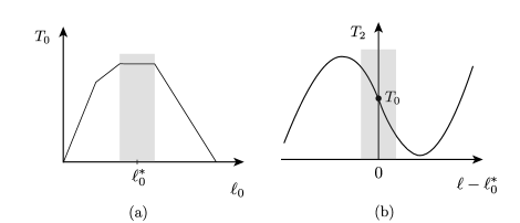
Figure 1: (a) Isometric tetanus: actively generated force $T_{0}$ as a function of the reference length $\ell_{0}$. (b) Quasi-equilibrium states $T_{2}$ reached from the stall state $T_{0}$ by fast shortenings or stretches. Highlighted are the main physiological regimes.

While the initial response $T_{1}$ can be clearly attributed to elasticity of myosin heads (cross-bridges) HS71 ; Lombardikappa , the recovered tension $T_{2}$ was shown to result from a conformational transition inside actin-bound myosin heads. During this re-equilibration transition, some of the cross-bridges switch (or fold) from pre- to post-power stroke state Irving92 ; Irving02 . The resulting massive conformational change is believed to be a purely mechanical process as it does not involve the un-binding of myosin heads from actin filamentsSheshka2020 .

Since the homogeneous state of isometric contractions is a stable equilibrium for the whole muscle fiber, the corresponding global elastic stiffness $dT_{2}/d\ell$ should be positive, and this is indeed what was observed in the pioneering experiments of Huxley and Simmons (HS) HS71 , see Fig. 2(b). They proposed a theoretical explanation for their measurements, arguing that the elementary force-generating units contain at least two structural elements connected in series HS71 . The first one is an elastic spring responsible for generating the tension $T_{1}$, which can be modeled as Hookean. The second is a bi-stable power stroke element that can be either in pre- or in post-power stroke position. HS modeled such element as a hard-spin variable representing the angular position of the myosin head with respect to actin. To ensure a collective response, individual myosin heads were assumed to be interacting non-locally, through rigid actin and myosin filaments. The resulting model placed the thermomechanical behavior of force generating units (half-sarcomeres) in a chemo-mechanical framework with pre- and post-power stroke conformations presented as chemical states. To obtain analytical results, HS used the Kramers approximation, but their model was recently generalized to account for the full-scale Langevin dynamics MT10 ; Marcucci2010 ; CT_PRE ; CT_JMPS .

The hard spin HS model with effectively paramagnetic-type mechanical interactions could reproduce the experimentally measured tension $T_{2}$ only if the stiffness of myosin heads was underestimated. If the correct value (2.7$\pm$0.9 pN.nm^-1, Brunello2014 ; Lombardikappa ; Linari19982459 ) is used, the HS model leads to the controversial prediction that the free energy of a half-sarcomere is a non-convex function of strain, which means, in particular, that the effective stiffness in the physiological stall force regime is negative HT96 ; Vilfan_BioPhys_2003 ; CAT_PRL , see Fig. 1(b) and Fig. 2(b). Behind such non-convexity is the insistence of the model on highly coherent mechanical response of interacting cross-bridges, which essentially precludes mixing of pre- and post-power stroke conformations. In other words, given the value of the environmental temperature, the assumed mean-field elastic interaction unambiguously points toward necessarily coherent response in the state of isometric contractions (stall conditions) with all cross-bridges either in the pre-power stroke or all in the post-power stroke conformation.

Figure 2: (a) Fast transients in mechanical experiments on single muscle fibers. In response to the length step $\delta\ell$, the tension first drops from $T_{0}$ to $T_{1}$ and then recovers a fraction of the initial tension, reaching the level $T_{2}$. (b) The recovered tension $T_{2}$ as a function of the imposed stretch $\delta\ell$. Solid curve shows the predictions of the HS model with realistic parameters: $a=10$nm, $\kappa_{0}=2$pN/nm, $T=277.15$K, $v_{0}=24.4$pN CT_ROPP_2018 ; borjadarocha_thesis . Data extracted from Huxley2000 ; Ford1981 ; Brunello_PNAS_2007

The non-positive-definiteness of the tangential elasticity in the constitutive model can potentially trigger spatial inhomogeneity at the scale of the whole muscle fiber. In particular, spatial inhomogeneity should be present in muscle fibers modeled as series connections of half-sarcomeres Vilfan_BioPhys_2003 ; Puglisi2000 . Individual half-sarcomeres will be then either entirely in pre- or post-power stroke configurations, which can be interpreted as a coexistence of pure phases. Even though this would lead to a realistically flat $T_{2}$ curve in the regime of isometric contractions, the homogeneous (affine) configurations will be unstable which suggests that the muscle fiber will be structurally highly inhomogeneous Vilfan_BioPhys_2003 ; Puglisi2000 ; Rassier2010 . The fact, that such inhomogeneity of ’muscle material’ has not been observed in experiments, stimulated theoretical efforts to account for physical factors ensuring the mixing of the pre- and post-power stroke configurations at the scale of individual half-sarcomeres.

Different mechanisms facilitating such mixing have been proposed in the literature. Efforts to suppress the instability of an affine response have started with the 1996 paper of Huxley and Tideswell (HT) HT96 , who suggested that the inter-mixing can be explained by the inherent randomness encapsulated in the actomyosin machinery. More specifically, the authors introduced the idea of a random attachment of the myosin motors along the actin monomer, resulting in a statistical distribution of the attachment positions spread over almost half of the actin diameter (5.5 nm). This assumption is realistic as the experiments involving electron microscopy Reedy_Taylor_PlosOne_2012 ; Tregear20043009 and X-ray diffraction Irving02 ; Reconditi2006 reveal a much more complex geometrical structure of the actomyosin complex than in the original HS model. Thus, myosin binds to actin only in specific target zones, which are not commensurate with the spacing of myosin heads. As a result, different binding sites are reached at different angles Tregear98 ; Tregear20043009 . As it was first realized by HTHT96 , the implied quenched disorder will compromise the coherent response in stall conditions. More recently, several other models addressed the same experimental data and successfully reproduced the positive slope of the $T_{2}$ curve, even though often without placing emphasis on the quenched disorder incorporated to overcome the original limitation of the HS model, see Piazzesi1995 ; Smith2008 ; SmithMijailovich2008 ; Caremani2015 and the references therein. The implications of the presence of disorder in the myosin attachment positions have been recently studied systematically in BRT_PRL_2019 . It was shown that having a structural disorder in the positions of myosin molecules relative to attachment sites can effectively convexify the elastic response and therefore flatten the $T_{2}$ curve. The rather unexpected result obtained in BRT_PRL_2019 was that a realistic disorder places a typical muscle system close to a thermodynamic critical point CAT_PRL . Despite these fascinating predictions, the idea of the functionality of geometrical disorder in the otherwise highly regular, crystal-type muscle architecture remains debatable. For instance, while the HT model postulates a Gaussian disorder with a particular variance, the realistic value of such temperature-like parameter is obscure; moreover, the actual statistical nature of the implied geometrical frustration is unknown. It is then possible, but not certain, that the existing incommensuration is sufficient to ensure the positive slope of the $T_{2}$ curve. The situation is somewhat similar to the original question faced by HS, of whether the value of the ambient temperature is sufficient to convexify their free energy.

Local inter-mixing of the pre- and post-power stroke conformations inside a single half-sarcomere can also be facilitated by an active process. As shown in SRT_PRE_2016 , the presence of correlated external excitations can generate positive active stiffness in the system, which otherwise has negative passive stiffness. In particular, such ATP-induced stiffening can overcome the negative stiffness of the original HS model, making the affine response of muscle fibers stable. Under this hypothesis, the coherency of the mean-field-dominated configurations can be broken because each element would be forced by active driving to stay away from a single energy well. Note that the implied active mixing of cross-bridge conformations is different from the passive ’melting’ taking over at high temperatures. Active driving, however, is energetically costly as it requires incessant ATP consumption. Therefore, it is still difficult to say how realistic is such stabilization scenario.

Given this uncertainty, it is natural to explore other possibilities for passive (rather than active) stabilization of affine response of muscle fibers in stall conditions. With this aim in view, we put forward in this paper a plausible hypothesis that the undesirable, highly coherent mechanical response of muscle half-sarcomeres may be compromised by the destabilizing short-range interaction between individual myosin heads. Such interaction would then compete with the stabilizing long-range elastic effect of the apparently semirigid filaments. To support this hypothesis, we recall in Sect. 2 some experimental observations and discuss the physical mechanisms which may ensure the destabilizing character of the short-range interaction between neighboring myosin heads.

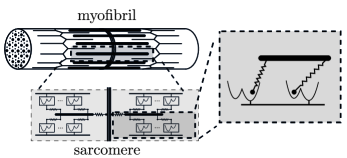
Figure 3: Half-sarcomere modeled as a parallel cluster of Huxley–Simmons units.

To rationalize the effect of the destabilizing short-range interactions, we use the general framework of the HS model. However, we now complement the mean-field interaction, favoring uniformity of micro-configurations, by the short-range interactions favoring the inter-mixing of pre- and post-power stroke states, see Fig.3. More specifically, we make the interaction of antiferromagnetic type between neighboring spins compete with the long-range paramagnetic-type interaction introduced in the original HS model. The ensuing 1D hard-spin model of a muscle half-sarcomere can be viewed as a version of the corresponding Ising model where various short- and long-range interactions are allowed to compete. Such competition can generate a rich repertoire of thermodynamic behaviors Nagle_PRA_1970 ; Nagle_JAP_1971 ; Kardar_PRB_1983 ; Nishino_PRB_2016 ; Campa_2019 and the goal of this paper is to explore different alternatives in the context of muscle mechanics. An additional complication is that the HS mean-field interaction makes the ensuing systems non-additive, which leads to ensemble inequivalence. In particular, the isometric and the isotonic mechanical responses will be necessarily different and would have to be treated separately Campa_2019 ; Mukamel_PhysicaA_2010 ; Barre_PRL_2001 ; Barre2002 . While the detailed nature of the postulated antiferromagnetic interactions still remains debatable (see Sect. 2 for details), we take in this paper a position that the quantitative consequences of the new hypothesis must be explored before any judgment of its relevance for the theory muscle contractions can be made.

We show that if the antiferromagnetic short-range interactions are sufficiently strong, the HS-type coherent single-state response can be indeed compromised. It is replaced by a non-HS response with cross-bridges in pre- and post-power stroke configurations finely mixed. Moreover, we show that in such regimes, the cross-bridges necessarily form a regular interdigitated pattern. The macroscopically homogeneous response of a muscle fiber is then recovered at the expense of the individual half-sarcomeres becoming maximally inhomogeneous.

One can say that the presence of short-range interaction is responsible for the emergence of a new energy well which stabilizes in this model the physiological state of isometric contractions. In addition to the coherent pre- and post-power stroke configurations anticipated by the original HS theory, the augmented model, accounting for short-range interactions, predicts the stability of configurations with pre- and post-power stroke cross-bridges finely mixed. In this new ’phase’, the overall stiffness of a half-sarcomere is positive, which suggests that it may be adequately representing the physiological state of isometric contractions. The macroscopically homogeneous response is then stabilized passively, in contradistinction with active stabilization studied in SRT_PRE_2016 .

We observe that additional energy wells (chemical states), different from the ones describing pre- and post-power stroke conformations, are sometimes introduced phenomenologically in chemo-mechanical models to ensure that the $T_{2}(\delta\ell)$ curve is sufficiently flat around the stall state, see, for instance, Marcucci_PLOS_2016 and the references cited therein. Instead, in the model with short-range antiferromagnetic interactions, the third energy well emerges directly from a micromodel without additional phenomenological assumptions.

The three-state systems of this type, which would be usually represented by a Potts model Ostilli2020 ; yeomans1992statistical , are characterized by a tricritical point separating the line of first- and second-order transitions. In our two-well microscopic model, where the third well appears after statistical averaging, the tricritical point arises as well, strongly influencing the corresponding equilibrium phase diagram. In addition to the ’coherent’ bi-stable phase predicted by the original HS theory and the ’melted’ phase appearing at high temperatures, such a phase diagram shows the existence of a domain with configurations of the antiferromagnetic type containing both pre- and post-power stroke cross-bridges. Acquiring such configurations may be physiologically beneficial for the system, which can then anticipate the necessity of either ultrafast contraction (global switching to post-power stroke state) or ultrafast stretching (global switching to pre-power stroke state). Moreover, we argue that a living system may benefit from being posed near such a singular point.

The paper is organized as follows. Section 2 discusses the feasible mechanisms behind the antiferromagnetic short-range interactions affecting neighboring myosin heads. The augmented HS model of a half-sarcomere is introduced in Section 3, where we study its behavior at zero temperature. Section 4 considers finite temperature effects and constructs the equilibrium phase diagram for the system in a hard device. The system in a soft device is studied in Section 5, where we also discuss the origin of the ensemble non-equivalence. We then specify in Section 6 the order parameters and study spatial correlations. The case study of two half-sarcomeres in series is presented in Section 7. Finally, in Section 8, we summarize our results.

2 Short-range interactions between neighboring myosin heads

We now turn to the physiological motivation for the introduction of the interacting heads hypothesis. Recall first that 150 nm long myosin II molecules can be viewed as narrow rods, each ending with two 10-15 nm globular domains (heads). The heads form projections and play the role of the enzymatic active sites, the ATPases, which are activated by six adjacent actin filaments to produce muscular force and movement. Instead, the myosin tails self-associate to form the backbones of thick filaments. The resulting rod packing is parallel with each crown (myosin head pairs) closely located to (and therefore elastically interacting with) several tails of the neighboring myosin molecules. The myosin II filaments arrangement is such that the crowns form 2D helical lattices. The individual helices are arranged with a 14.3-nm separation between crowns and a 42.9-nm helical repeat Squire2017 , see Fig. 4(a).

Since the conformational change inside myosin heads produces an extension of the order of $\sim 10$ nm Higushi_Nature2017 , the size of the working stroke is comparable to the distance between consecutive myosin heads along the helix. Therefore, whether a particular myosin head is in pre- or post-power stroke position may influence its neighbors’ state, and the local patterning may be at least partially guided by such interaction. Depending on their spatial configurations, the two successive crowns can potentially interact either directly (sterically) or indirectly through the adjacent tropomyosin–troponin regulatory units Razumova_BiophysJournal_2000 or through other environmental proteins Squire2009 .

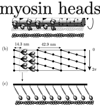
Figure 4: (a) Arrangement of the myosin crowns on the cylindrical surface of the myosin backbone. (b) Coaxial helices on flattened cylinder with emphasized pairs of myosin heads. (c) HS stylized model of a half-sarcomere with each cross-bridge effectively representing three myosin crowns. The corresponding actin backbone is an effective representation of the six actin (thin) filaments comprising the matching stereotypical units for each thick filament.

The short-range interaction between the crowns may involve first and second heads. It is known, for instance, that the regularly organized helical myosin head structures can be thought as stabilized by head-to-head interactions, however, the role of the second head in the dimeric myosin II molecule remains enigmatic. For instance, there is a range of experimental results suggesting negative cooperativity between the two heads, which implies that binding of one head to actin inhibits binding of the other Mansson2015 . The two heads may then form an asymmetric structure with the overall dimension along the helix comparable with the distance between neighboring crowns Tanner_PLOS_2007 . Thus, if one of the heads in the contracting state is oriented almost perpendicular to the fiber axis, the partner head would be stretched axially Oshima_2007 .

In Fig. 4(a,b), we show the schematic 3D configuration of the crowns and illustrate the model reduction approach employed in the derivation of the simplest HS model. The reduced model shown in Fig. 4(c) introduces an effective cross-bridge as collective representation of several laterally separated crowns. Each ’collective’ myosin head is interacting with a similarly schematized actin filament, representing six separate real active filaments. Such model neglects the presence of two myosin heads and does not resolve the actual spatial configuration of the neighboring crowns. While this model accounts for the elastic interaction between the effective cross-bridges and the rigid filaments, it clearly underestimates the possibility of the geometrically allowed short-range interaction between the neighboring effective cross-bridges.

Spatial configuration of contracting half-sarcomeres can be also influenced by the elastic coupling between myosin heads along the compliant myofilament lattice Hill_PNAS_1980 ; Piazzesi1995 ; Hancock1997 ; Razumova_BiophysJournal_2000 ; Rice_BioPhysJournal_2003 ; Mijailovich_BiophysJournal_1996 . The presence of such elastic interaction would imply that cross-bridges do not operate independently while generating force Daniel_Biophys_1998 ; Chase2004 ; Campbell2006 . In Ford1981 , a continuum extension of the HS model was proposed in which the compliance of the thick and thin filaments was actually taken into account. This model was further developed in Mijailovich_BiophysJournal_1996 , where the authors explicitly argued that "the local behavior of one myosin head must depend on the of neighboring attachment sites." The effects of stochasticity in this model were studied in Campbell2006 .

More recently, a discrete model dealing with an array of motors and also accounting for compliance of discretized myofilaments was considered in Powers2020 . A minimal representation of this discrete model of a half-sarcomere, where $N$ effective cross-bridges are protruding periodically from an elastic backbone and are bound to a rigid actin filament, is shown in Fig. 5. In mechanical terms, it can be viewed a mass–spring chain containing $N$ nodes that are linked to an elastic (Winkler) foundation. Neglecting the conformational bi-stability, one can assume that springs are linear with the reference length $a=L/N$, where $L$ is the length scale of a half-sarcomere. Such model was probably first introduced by De Gennes in his pioneering study of the mechanical response of two-stranded DNA DEGENNES20011505 .

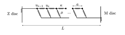
Figure 5: A schematic mechanical model of a thick filament as an array of interacting linear springs coupled to a Winkler foundation. The cross-bridges are represented by linear springs with common elasticity $\mu$. Each cross-bridge interacts elastically with each of its neighbors via a linear spring with modulus $\kappa$.

To assess the nature of the effective nearest neighbor (NN) interaction between the nodes, we can reduce the ’double chain’ model shown in Fig. 5 to a ’single chain’ minimal model. To this end, we introduce the displacements of the nodes $u_{i}$ and write the energy of the system in the form

$$E(\bm{u})=\frac{1}{N}\sum_{i=1}^{N}\frac{\kappa}{2}\left(\frac{u_{i}-u_{i-1}}{a}\right)^{2}+\frac{1}{N}\sum_{i=1}^{N+1}\frac{\mu}{2}u_{i}^{2},$$ (1)

where $\kappa$ is the stiffness of the horizontal springs and $\mu$ is the (shear) modulus of the vertical (leaf) springs. While the first term in Eq. (1) describes the compliance of the filaments, the second term represents the elasticity of the individual cross-bridges. We note that for simplicity, the thick filament is assumed to be rigid.

In the limit $a\to 0$ and $N\to\infty$, the discrete model (1) can be approximated by the continuum model with energy

$$E(u)=\int_{0}^{L}\left(\frac{\kappa}{2}w^{2}+\frac{\mu}{2}u^{2}\right)dx,$$ (2)

where $x\in(0,L)$ is the spatial coordinate, $u(x)$ is the horizontal displacement field, and $w(x)=\partial_{x}u(x)$ is the continuum strain field. We can assume that the system is subjected to isometric loading (hard device) with the total displacement prescribed $\int_{0}^{L}wdx=d$.

To rewrite the energy (2) in terms of the local strain field $w$ only, we can follow Ren2000 and define the characteristic (indicator) function $\xi_{y}\mathrel{\mathop{\mathchar 58\relax}}x\to\{0,1\}$ such that for $x\leq y$ : $\xi_{y}(x)=1$, and for $x>y$ : $\xi_{y}(x)=0$. If we then assume for determinacy that $u(0)=-d/2$, and $u(L)=d/2$, we can write

$$\begin{split}\int_{0}^{L}\mu u^{2}dx&=\mu\int_{0}^{L}\left[\int_{0}^{L}\xi_{x}(y)w(y)dy-\frac{d}{2}\right]^{2}dx\\ &=\mu\int_{0}^{L}\left[\int_{0}^{L}\left(\xi_{x}(y)w(y)-\frac{1}{2}w(y)\right)dy\right]^{2}dx\\ \end{split}$$ (3)

Then, noticing that $\int_{0}^{L}\left(\xi_{x}(y)-\frac{1}{2}\right)\left(\xi_{x}(z)-\frac{1}{2}\right)dx=\frac{L}{4}-\max\{x,y\}+\frac{1}{2}(x+y),$ we can rewrite the energy (2) in the form

$$E(w)=\int_{0}^{L}\kappa w^{2}dx+\mu\int_{0}^{L}\int_{0}^{L}K(x,y)w(x)w(y)dxdy$$ (4)

where $K(x,y)=\frac{L}{4}-\max\{x,y\}+\frac{1}{2}(x+y)$ is the interaction kernel, which is defined on the square domain $[0,L]\times[0,L]$.

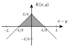
Figure 6: The dependence of the kernel function $K(x,y)$ on $x-y$. For $|x-y|\leq L/2$, we observe antiferromagnetic-type behavior with $K\geq 0$.

In Fig. 6, we illustrate the structure of the kernel function $K(x,y)$ showing its behavior along the $x-y$ diagonal direction. Note that $K(x,y)>0$ for small values of $|x-y|$, which is the range corresponding to short-range interactions. Therefore, the configurations with $w(x)$ and $w(y)$ having alternating signs at neighboring points $x$ and $y$ will have lower energy $E$ vis a vis the configurations with locally homogeneous strain. As a result, the system with the energy (4) will be driven toward configurations with locally alternating strains ($w>0$ for stretching and $w<0$ for compression). Such configurations can be interpreted as having antiferromagnetic order chaikin1995principles . In the presence of nonlinear terms in the energy describing conformational change (power stroke), the underlying effective antiferromagnetic-type short-range elastic interaction between neighboring nods (describing myosin heads) can be expected to facilitate the formation of fine mixtures of cross-bridges in pre- and post-power stroke configurations.

We can conclude that the account of steric effects and filament extensibility can, in principle, bias the relative displacements of the neighboring cross-bridges toward non-uniformity Mijailovich_BiophysJournal_1996 ; Daniel_Biophys_1998 . Such interactions make the local conformational state of an attached myosin head affected by the conformational state of the neighboring heads. Moreover, it is known Ren2000 that the account of the antiferromagnetic interaction can make the coherent configurations with larger averaged spacing energetically less preferable than the ’closed packed’ interdigitated configurations with pre- and post-power stroke cross-bridges periodically patterned at the smallest available scale.

Consider now the issue of conformational homogeneity in the mechanical response of single half-sarcomeres. It is well known that in isometrically contracting muscle myofibrils, the cross-bridges move through the reversible power stroke asynchronously and assume, at any moment in time and any given location, both conformations MIDDE20111024 ; Hirose1993 ; Reedy_2000 ; Thomas_BiophysicalJornal_1995 . In particular, there is evidence that at the steady-state plateau of isometric tetanus, see Fig. 1(a), the individual myosin motors are in different conformations, which is sometimes interpreted as a ’state of disorder.’ However, the cross-bridges can potentially get synchronized spatially and temporarily in response to very rapid stretches or slacks and, in this sense, the fast force recovery is sometimes interpreted, in accordance with HS theory, as a disorder-to-order transition Thomas_BiophysicalJornal_1995 .

In any case, such interpretations remain qualitative since the usual mechanical and structural measurements at the single half-sarcomere level address populations of myosin motors. This makes it difficult to follow the change in conformation of individual cross-bridges and quantify the process of stress-induced spatial synchronization Lombardikappa . Still, specially designed X-ray experiments can provide at least some access to the spatial distribution of the myosin motors. For instance, one can use for this purpose the width of the third-order myosin-based meridional reflection (M3 reflection) as it can be related to the number of myosin motors in the pre-power stroke state. Moreover, the splitting of the M3 reflection can be linked to the distance between the two arrays of myosin motors in pre- and post- power stroke states Reconditi_PNAS_2017 . Based on these and other experimental approaches, it was suggested that while at loads closer to stall conditions myosin motors are broadly distributed, at lower loads they proceed through the stroke almost collectively Piazzesi1992 ; Reconditi_Nature_2004 .

Such measurements, however, still provide information only about the homogenized state. If, for instance, the averaged observed state in the quenched configuration is between pre- and post-power stroke, they do not reveal the actual geometrical (ordered) pattern behind this averaged behavior.

To summarize, the assumption of the original HS model that individual myosin heads interact only through the thick filament, modeled as a rigid backbone, does not allow one to make any conclusions about the spatial organization of pre- and post-power stroke cross-bridges inside a single half-sarcomere. To quantify the conjectured self-organization of the closely interacting myosin heads into alternating conformational patterns, it is necessary to go beyond the class of HS type mean-field models and account explicitly for short-range interactions between neighboring cross-bridges. Such in silico modeling will allow one to make quantitative predictions which are needed to either confirm or reject the hypothesis of antiferromagnetic-type nearest neighbor interactions.

3 The model of a half-sarcomere

Following HS, we model a half-sarcomere as a collection of $N$ interacting cross-bridges, but we supplement the mean-field interaction introduced of HS by a competing short-range interaction.

The energy of non-interacting cross-bridges can be written as

$$\sum_{i}^{N}V(X_{i}),$$

where $i=1,\dots,N$ and $V(X_{i})$ is a double-well energy of a single cross-bridge, see Fig. 3. We assume for analytical simplicity that the two conformational positions of the myosin head are represented by the hard-spin variable $X_{i}$ so that in the pre-power stroke state $X_{i}=0$, and in the post-power stroke state $X_{i}=-a$, where $a$ is the amount by which the myosin head pulls the actin during the power stroke. We set that $V(X_{i})=(a+X_{i})V_{0}$ which shows that the pre-power stroke conformation has higher energy than the post-power stroke conformation with the energy bias equal to $V_{0}$ (in the units of force), see Fig. 7. Despite the overall passive (ATP indifferent) nature of the HS model, the parameter $V_{0}$ has an active origin as it is ultimately responsible for the generation of the tension $T_{0}$ in the stall state (state of isometric contractions).

In the HS model, each cross-bridge is connected to a common rigid backbone through an elastic spring $\kappa_{0}$ placed in series with a bi-stable unit. The backbone is characterized by a single variable $Y$, and the corresponding interaction energy is of mean-field type

$$\sum_{i}^{N}\frac{\kappa_{0}}{2}(Y-X_{i})^{2},$$

where $\kappa_{0}>0$ is a parameter stabilizing homogeneous distribution of cross-bridge configurations.

In addition to this interaction, we assume that each element also interacts harmonically with its nearest neighbors through the energy term

$$\sum_{i}^{N}\frac{\kappa_{J}}{2}(X_{i+1}-X_{i})^{2},$$

where $\kappa_{J}$ is the corresponding linear stiffness. The various potential sources of such short-range interaction were discussed in detail in Sect. 2. In particular, we showed there that to adequately account for compliance of the filaments and to produce the anticipated destabilizing effect on the homogeneous distribution of cross-bridges, such short-range interaction should be of antiferromagnetic type. This means that the parameter $\kappa_{J}$ should be negative.

Finally, we assume that the whole half-sarcomere is loaded through an elastic spring with stiffness $\kappa_{f}>0$, representing the combined elasticities of actin and myosin filaments. When the system is loaded in a hard device, an imposed displacement $Z$ is applied to the external spring giving the contribution to the energy

$$\sum_{i}^{N}\frac{\kappa_{f}}{2N}(Z-Y)^{2}.$$

Figure 7: (a) Schematics showing two neighboring cross-bridges in different conformational states, (b) Huxley–Simmons (HS) model of a single cross-bridge. The two conformational states of the myosin head are represented by the spin variable $x$, while the lump elasticity of the whole cross-bridge is represented by the parabolic potential acting on the continuous variable $y$.

To non-dimensionalize the problem, we define the reference length $a$ and normalize the spatial variables accordingly: $x_{i}=X_{i}/a$, $y=Y/a$ and $z=Z/a$. Note that now the variable $x_{i}$ takes values 0 and -1 for the pre- and post-power stroke, respectively. Using $\kappa_{0}a^{2}$ as the scale of the energy, we obtain in dimensionless variables

$$\begin{split}E(\bm{x},y,z)&=\sum_{i}^{N}\left[(1+x_{i})v_{0}+\frac{1}{2}(y-x_{i})^{2}+\frac{\lambda_{J}}{2}(x_{i+1}-x_{i})^{2}+\frac{\lambda_{f}}{2}(z-y)^{2}\right],\end{split}$$ (5)

where $v_{0}=V_{0}/(\kappa_{0}a)$ is the non-dimensional energy bias. We consider periodic boundary conditions: $x_{N+1}=x_{1}$, however, in the thermodynamic limit $N\to\infty$; the choice of this type of boundary conditions becomes irrelevant yeomans1992statistical ; goldenfeld1992lectures . The ensuing problem contains two dimensionless parameters $\lambda_{J}=\kappa_{J}/\kappa_{0}$ and $\lambda_{f}=\kappa_{f}/(N\kappa_{0})$.

To reveal the main effect, it is sufficient to analyze the system at zero temperature. To obtain the ground state, we first eliminate $y$ using the condition $\partial E/\partial y=0$, which is equivalent to

$$y=\frac{\lambda_{f}z}{1+\lambda_{f}}+\frac{1}{N(1+\lambda_{f})}\sum_{i}x_{i}.$$ (6)

The relaxed energy is of Ising form with both mean-field and short-range interactions:

$$\begin{split}E(x_{i},z)=-\frac{K}{2N}\sum_{i,j}x_{i}x_{j}-\lambda_{J}\sum_{i}x_{i}x_{i+1}-h(z)\sum_{i}x_{i}+c(z).\end{split}$$ (7)

where $1/K=1+\lambda_{f}$ and

$$h(z)=\frac{\lambda_{f}z}{1+\lambda_{f}}-v_{0}+\lambda_{J}+\frac{1}{2},\,\,\,\,c(z)=\frac{N\lambda_{f}z^{2}}{2(1+\lambda_{f})}+Nv_{0}.$$

Since this energy is quadratic in $z$ at a given $x_{i}$, the minimization over $x_{i}$ reduces to the choice among a finite number of parabolas.

Depending on the values of $\lambda_{J}$ and $\lambda_{f}$, the global minima correspond to either pure phases, with all cross-bridges synchronized in the same conformational state (pre- or post-power stroke), or to a mixed phase with lattice-scale oscillations between the two conformational states. At a not too negative value of $\lambda_{J}$, the energy minimizing phase is ferromagnetic with pre- or post-power stroke state dominating depending on whether the system is stretched or compressed. At sufficiently negative $\lambda_{J}$, when destabilizing short-range interactions are strong, the unstressed system can also be in an antiferromagnetic state when neighboring cross-bridges are in opposite conformational states.

The phase diagram, revealing the structure of the ground state in the unstressed state, is presented in Fig. 8(a). The boundary separates the antiferromagnetic (mixed) and ferromagnetic (pure) ground states. We assumed here, for simplicity, that the unstressed state describes the stall condition and also arbitrarily set that in this state, the distribution of pre- and post-power strokes cross-bridges is 50-50 . We therefore have the stall state at $z=z_{0}=(1+1/\lambda_{f})v_{0}-1/2$ where post- and pre-power stroke conformations have the same energy. Note that at $z=z_{0}$ the energies of pure and mixed configurations become equal if $1/\lambda_{J}=-4(1+\lambda_{f}).$ At

$$\lambda_{J}<-\frac{1}{4(1+\lambda_{f})}$$

the equilibrium configuration in stall conditions is mixed, while it is coherent (all cross-bridges are either pre- or post-power stroke) otherwise. In the limiting case $\lambda_{f}\to\infty$, when cross-bridges interact only at short-range, the transition occurs at $\lambda_{J}=0$. In the other limiting case $\lambda_{f}\to 0$, the crossover between ferromagnetic and antiferromagnetic phases takes place at $\lambda_{J}=-1/4$.

We now compare the energies of different spatial distributions $x_{i}$ at $z=z_{0}$. In the FM phase, any of the mixed configurations will have higher energy than one of the pure configurations $E_{mixed}(z=z_{0})>E_{pure}(z=z_{0})$, while in the AFM phase $E_{mixed}(z=z_{0})<E_{pure}(z=z_{0})$. Here $E_{pure}$ can be taken as the energy of a configuration with either all pre- or all post-power stroke cross-bridges because at $z=z_{0}$ they are equal.

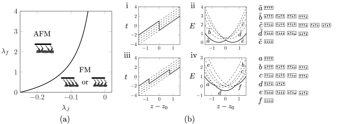
Figure 8: (a) Zero temperature phase diagram for a half-sarcomere in the stall state $z=z_{0}$. (b) Energy and tension of a system of $N=4$ cross-bridges. The thick solid line represents the global minimum of the energy (ground state), while the dashed line represents the local energy minima (metastable states). In i–ii, we illustrate the ferromagnetic (FM) part of the phase diagram (corresponding to $\lambda_{f}=1$, $\lambda_{J}=0$), and in iii–iv, the antiferromagnetic (AFM) part (corresponding to $\lambda_{f}=1$, $\lambda_{J}=-0.5$). In (b), each metastable branch is associated with a particular micro-configuration, which is illustrated in the right column. The ’up/down arrows represent pre/post power stroke states.

In Fig. 8(b)(ii, iv), we show the energies of local and global minimizers $E(z)$ corresponding to mixed (alternating pre- and post-power stroke states) and pure (fully synchronized) configurations that are parameterized by $z$. The corresponding branches of tension–elongation curves $t=dE/dz$ are shown in Fig. 8(b)(i,iii).

It is interesting that in the tension curves 8(b)(i, iii), different metastable branches are uniquely characterized by the total amount of spins in either pre- or post-power stroke, which means that from developed tension alone we cannot distinguish spatial organization. To this end, we need to turn to the energy function. The reason comes directly from the energy (7) where all $z$ related terms are in $h$ and $c$, which means that both short- and long-range terms ($J$ and $\lambda_{J}$, respectively) are $z$ insensitive, and only the average ’magnetization’ $\sum_{i}x_{i}$ interacts with the loading device. However, ultimately the choice of the most stable branch is dictated by the energy.

We also note that in the ferromagnetic phase, the macroscopic stiffness in the stall state is equal to minus infinity. In the antiferromagnetic phase, the transition between the two pure states is smoothed, but the stiffness in the stall state remains to be equal to minus infinity. This means that the formal ’stabilization’ of this state is impossible at zero temperature.

To summarize, the analysis of the zero temperature system shows that due to the mean-field nature of ferromagnetic interactions, the preferred behavior is coherent with fully relaxed energy remaining non-convex and the corresponding stiffness taking negative values. Adding sufficiently strong short-range antiferromagnetic interactions partially convexifies the relaxed energy; however, negative stiffness persists.

4 Equilibrium response

To study the equilibrium response of the system at finite temperature $\theta$, we need to compute its free energy. The partition function in the hard device ensemble (controlled displacement) is,

$$\mathcal{Z}(\beta,z)=\int dy\sum_{\{x\}}e^{-\beta E(x_{i},y,z)},$$

where the summation is over $x_{i}=\{0,-1\}$ for all $x_{i}$; we also use the standard notation $\beta=\kappa_{0}a^{2}/k_{B}\theta$, where $k_{B}$ is the Boltzmann constant. Since $\sum_{i}x_{i}^{2}=-\sum_{i}x_{i}$, we can write

$$\begin{split}\mathcal{Z}(\beta,z)&=\int dye^{-\beta N\varphi(y,z)}\mathcal{Z}_{0}(\beta,y),\end{split}$$ (8)

where $\varphi(y,z)=\frac{\lambda_{f}}{2}(z-y)^{2}+v_{0}+\frac{y^{2}}{2}$ and the function $\mathcal{Z}_{0}(\beta,y)$ is the partition function for an Ising ring goldenfeld1992lectures :

$$\begin{split}\mathcal{Z}_{0}(\beta,y)&=\sum_{\{x\}}\exp\left[\beta J\sum_{i}x_{i}x_{i+1}+\beta H\sum_{i}x_{i}\right],\end{split}$$ (9)

where, $J=\lambda_{J}$ and $H(y)=\lambda_{J}+y+1/2-v_{0}$. The equilibrium behavior of this system without short-range interactions ($\lambda_{J}=0$) was studied in CT_PRE .

Figure 9: Different solutions of the self-consistency condition (14) correspond to interactions of different curves with an inclined straight line. In Phase I, there are three solutions (two energy minima, two symmetric ground states), in Phases II and III, there are five solutions (three energy minima with either one or two ( symmetric) ground states), and in Phase IV, the solution is unique (single energy minimum which is also the ground state).

To compute $\mathcal{Z}_{0}(\beta,y)$ we can use the transfer matrix method Campa_2019 ; christensen2005complexity . The idea is to represent this partition function as a product of equal matrices yeomans1992statistical ; goldenfeld1992lectures . Consider the matrix

$$\bm{T}=\left(\begin{array}[]{cc}1&e^{-\frac{\beta H}{2}}\\ e^{-\frac{\beta H}{2}}&e^{\beta(J-H)}\end{array}\right).$$ (10)

Then, $\mathcal{Z}_{0}=\operatorname{Tr}(\bm{T}^{N}),$ and since $\bm{T}$ is real and symmetric, it can be diagonalized with the eigenvalues

$$\lambda_{1,2}=e^{-h}\left[\cosh h\pm\sqrt{\sinh^{2}h+e^{-\beta J}}\right],$$ (11)

where $h=\frac{\beta}{2}(H-J)$. Using the invariance of the trace, we obtain $\mathcal{Z}_{0}=\lambda_{1}^{N}+\lambda_{2}^{N}.$ If we now assume that $\lambda_{1}>\lambda_{2}$ and take the thermodynamic limit $N\rightarrow\infty$, we obtain $\mathcal{Z}_{0}\approx\lambda_{1}^{N}\left[1+\mathcal{O}(e^{-\alpha N})\right],$ where $\alpha\equiv\log(\lambda_{1}/\lambda_{2})$ is a positive constant. Using the Laplace method, we finally obtain

$$\mathcal{Z}(\beta,z)\sim\min_{y}\left\{e^{-\beta\varphi(y,z)}\lambda_{1}(y)\right\}.$$ (12)

The free energy density is $\mathcal{F}(\beta,z)=-\frac{1}{N\beta}\log\mathcal{Z}(\beta,z)$. In the thermodynamic limit, we can write

$$\begin{split}\mathcal{F}(\beta,z,y)&=\frac{\lambda_{f}}{2}(z-y)^{2}+v_{0}+\frac{y^{2}}{2}+\frac{g(y)}{\beta}-\frac{1}{\beta}\log\left[\cosh g(y)+\sqrt{e^{-\beta\lambda_{J}}+\sinh^{2}g(y)}\right].\end{split}$$ (13)

where $g(y)=\frac{\beta}{2}(y+1/2-v_{0})$. By solving a transcendental equation $\partial\mathcal{F}(\beta,z,y)/\partial y=0$, we obtain the self-consistency relation $y_{*}=\Psi(\beta,z,y_{*})$ illustrated in Fig. 9 with the function $\Psi(y_{*})$ known explicitly

$$\Psi(\beta,z,y)=\lambda_{f}(z-y)-\frac{1}{2}+\frac{1}{2}\frac{\sqrt{e^{-\beta\lambda_{J}}+\sinh^{2}g(y)}}{e^{-\beta\lambda_{J}}\operatorname{csch}g(y)+\sinh g(y)}.$$ (14)

As we show in Fig. 9, the equation (14) may have more than one solution, which reflects the non-convexity of the partial free energy $\mathcal{F}(\beta,z,y)$ The parametric dependence of this energy is illustrated in Fig. 10 for the stall state with $z=z_{0}$. Four different phases can be identified on the plane ($\lambda_{J},1/\beta$). The zero temperature phase diagram shown in Fig. 8(a) corresponds to the first-order transition boundary separating Phases II and III and is represented in Fig. 10 by its section at $\lambda_{f}=1$.

Figure 10: (a) Phase diagram for the system in the hard device with $z=z_{0}$. Parameters: $\lambda_{f}=1$, $v_{0}=0$. The transition between Phases I and IV is continuous (bold solid line) down to the tricritical point TCP, where it becomes first-order (dashed line). The dotted lines are spinodal boundaries. The different phases are illustrated in the right column, where we show the dependence of the partial free energy $\mathcal{F}$ on the internal variable $y$.

In the domain with low temperature and dominating mean-field interactions, we observe Phase I. In this phase, two pure states coexist, but at any instant of time, all cross-bridges are either in pre- or post-power stroke conformations. In other words, in stall conditions, the system in Phase I randomly switches between these two states. Each of these transitions takes place coherently, with all cross-bridges changing their state cooperatively. In the high-temperature domain and still dominating mean-field interactions, we observe Phase IV, where all cross-bridges switch randomly and independently between pre- or post-power stroke conformations. Phase IV is separated from Phase I by a second-order phase transition, analogous to the usual order–disorder transition in magnetics.

At low temperatures and strong short-range antiferromagnetic interactions, we observe the appearance of Phases II and III, where in addition to pure states, there is also a mixed state where neighboring cross-bridges have different conformations. In Phase II, the mixed state is metastable, and the equilibrium states are the pure ones, while in Phase III, the equilibrium state is the mixed one. Phases II and III are separated by the line of first-order phase transition, which meets the second-order phase transitions line separating Phases I and III at a tricritical point.

To summarize, when the short-range interactions are sufficiently strong and the temperature is sufficiently low, we observe a new feature in the system’s behavior: An antiferromagnetic state becomes stable in the stall regime $z=z_{0}$ (our Phase III). In other low-temperature Phases I and II, the stall state must necessarily involve random coherent conformational changes involving all cross-bridges simultaneously. At high temperatures, the paramagnetic phase dominates where all cross-bridges fluctuate randomly and independently over the whole energy landscape with neither pre- or post-power stroke stated clearly discernible. We have seen that by increasing $\lambda_{J}$ in the positive direction, we effectively decrease the temperature by favoring cooperativity and effectively destabilizing the homogeneous state at $z=z_{0}$. Instead, by increasing $\lambda_{J}$ in the negative direction, we disfavor coherent fluctuations between pure states at $z=z_{0}$ and stabilize instead non-fluctuating macroscopically homogeneous state, which we later show to be microscopically a fine lattice-scale mixture of pre- and post-power stroke conformations.

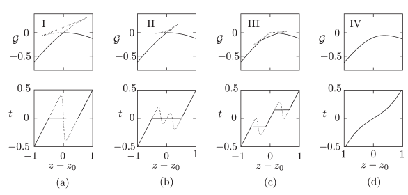
Figure 11: The equilibrium free (Helmholtz) energy–strain relation in the hard device and the corresponding tension–strain relation. (a) Phase I: $\lambda_{J}=0$, $\beta=50$; (b) Phase II: $\lambda_{J}=-0.1$, $\beta=50$; (c) Phase III: $\lambda_{J}=-0.25$, $\beta=50$; and (d) Phase IV: $\lambda_{J}=-0.25$, $\beta=8$. Other parameters: $\lambda_{f}=1$ and $v_{0}=0$. Solid curves correspond to ground states. With dotted lines, we show for convenience the unstable equilibria which have nothing to do with the equilibrium response but provide information about the energy barriers.

We now turn to the parametric behavior of the equilibrium free energy $\mathcal{F}(z)=\mathcal{F}(z,y_{*}(z))$. Knowing this energy, one can also compute the equilibrium tension $t(z)=d\mathcal{F}(z)/dz=d\mathcal{F}(z,y_{*}(z))/dz=\partial\mathcal{F}(z,y_{*}(z))/\partial z=\lambda_{f}(z-y_{*}(z)),$ where we temporarily omitted dependence on $\beta$. The behavior of the functions $\mathcal{F}(z)$ and $t(z)$ in different phases is illustrated in Fig. 11. Note that in (a) and (b) (Phases I and II), the free energy is non-convex at $z=z_{0}$, and the corresponding stiffness is negative. Instead, in (c) and (d) (Phases III and IV), the stall state is associated with the point of convexity of the equilibrium energy, and the corresponding stiffness is positive. However, if in Phase IV we deal with entropic stabilization at the expense of an identifiable conformational state, in Phase III, we encounter macroscopic homogeneity with the perfect antiferromagnetic order where each cross-bridge maintains its conformation with one half of them being in pre- and another half in post-power stroke state.

To obtain an analytical expression for the line of critical points (and ultimately for the tricritical point where it ends) on the phase diagram shown in Fig. 10, we can build around it a polynomial, Landau type expansion goldenfeld1992lectures ; pathria1996statistical .

To define an order parameter, we recall that, according to (6), the average value of the microscopic spin variable $\left<x\right>=N^{-1}\sum_{i}x_{i}$ is related to the macroscopic variable $y$ through the relation $\left<x\right>=(\lambda_{f}+1)y-\lambda_{f}z.$ Since $E(x_{i}=0,z_{0})=E(x_{i}=-1,z_{0})$, in stall conditions $z=z_{0}$ the fraction of post-power stroke elements should be equal to the fraction of pre-power stroke elements, which suggests that $\left<x\right>(\beta,z_{0})=-1/2$. Then, the natural order parameter is $\phi=2\left<x\right>+1$, or equivalently, $\phi=2(\lambda_{f}+1)y-2\lambda_{f}z+1.$ It now represents the fraction of elements in either conformation, meaning that with $\phi=1$ all units are in the pre-power stroke, and with $\phi=-1$ in the post-power stroke configuration. Finally, $\phi=0$ means that there are equal number of elements in both conformations.

The marginal free energy at $z=z_{0}$ can be now written in terms of $\phi$

$$\begin{split}\mathcal{F}(\beta,\phi)=\frac{1}{2}\left(v_{0}+\frac{1}{2}\right)^{2}+\frac{v_{0}^{2}}{2\lambda_{f}}+\frac{\phi^{2}}{8(1+\lambda_{f})}-\frac{1}{\beta}\log\left[\cosh\frac{\beta\phi}{4(1+\lambda_{f})}+\sqrt{e^{-\beta\lambda_{J}}+\sinh^{2}\frac{\beta\phi}{4(1+\lambda_{f})}}\right].\end{split}$$ (15)

The corresponding self-consistency relation expressed in terms of $\phi_{*}$ takes the form

$$\phi_{*}=\frac{\sinh\frac{\beta\phi_{*}}{4(1+\lambda_{f})}}{\sqrt{e^{-\beta\lambda_{J}}+\sinh^{2}\frac{\beta\phi_{*}}{4(1+\lambda_{f})}}}.$$ (16)

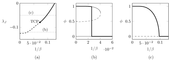
Figure 12: (a) Phase diagram in the hard device with $z=z_{0}$. Second-order transitions are shown by a solid bold line, first-order phase transitions by a dashed bold line. The dotted lines indicate the locations of the two representative sections shown in (b) and (c). (b) First-order phase transition, $\lambda_{J}=-0.12$. Thin solid lines correspond to metastable states, dash-dotted line—to unstable states; (c) Second-order phase transition, $\lambda_{J}=-0.05$. The dash-dotted line corresponds to unstable states.

In Fig. 12 (b) and (c), we show the behavior of the function $\phi_{*}(\beta)$ around the lines of first- and second-order phase transitions (critical points), respectively, shown in Fig. 12(a). Our goal now is to capture the line of second-order phase transitions separating Phases I and IV. To this end, it is sufficient to perform the Taylor expansion of the free-energy Eq. (15) around $\phi=0$. We obtain the expression $\tilde{\mathcal{F}}(\beta,\phi)=a_{0}+a_{2}\phi^{2}+a_{4}\phi^{4}$ where

$$a_{0}=\frac{1}{2}\left(v_{0}+\frac{1}{2}\right)^{2}+\frac{v_{0}^{2}}{2\lambda_{f}}-\frac{\log\left(\sqrt{e^{-\beta\lambda_{J}}}+1\right)}{\beta},$$ (17a)

$$a_{2}=\frac{1}{32(1+\lambda_{f})}\left[4-\frac{\beta}{(1+\lambda_{f})\sqrt{e^{-\beta\lambda_{J}}}}\right],a_{4}=\frac{\beta^{3}\left(3e^{\beta\lambda_{J}}-1\right)}{6144(1+\lambda_{f})^{4}\sqrt{e^{-\beta\lambda_{J}}}}.$$ (17b)

The approximate self-consistency relation $d\tilde{\mathcal{F}}/d\phi=0$ gives either $\tilde{\phi}=0$ or

$$\tilde{\phi}=\pm 4(1+\lambda_{f})\sqrt{\frac{6\beta-24(\lambda_{f}+1)\sqrt{e^{-\beta\lambda_{J}}}}{\beta^{3}\left(3e^{\beta\lambda_{J}}-1\right)}}.$$ (18)

The critical inverse temperature is implicitly given by relation $4(1+\lambda_{f})\sqrt{e^{-\beta_{c}\lambda_{J}}})=\beta_{c}$, which corresponds to $a_{2}=0$. In the limit $\lambda_{J}\rightarrow 0$, we obtain $\beta_{c}=4(1+\lambda_{f})$.

To locate the tricritical point (TCP) where the second-order phase transition becomes the first-order phase transition, we need to use the sixth-order expansion in the order parameter $\tilde{\mathcal{F}}(\beta,\phi)=a_{0}+a_{2}\phi^{2}+a_{4}\phi^{4}+a_{6}\phi^{6}$ where the additional coefficient is

$$a_{6}=\frac{\beta^{5}\left(30e^{\beta\lambda_{J}}-45e^{2\beta\lambda_{J}}-1\right)}{2949120\sqrt{e^{-\beta\lambda_{J}}}}.$$ (19)

The tricritical point can be linked to the vanishing of the second- and fourth-order terms in the expansion. Therefore, we obtain two equations $\beta=4(1+\lambda_{f})e^{-\beta\lambda_{J}/2}$ and $e^{-\beta\lambda_{J}/2}=\sqrt{3}$. Their solution can be found explicitly $\beta_{TCP}=4(1+\lambda_{f})\sqrt{3}$ and $\lambda_{JTCP}=-\log 3/4(1+\lambda_{f})\sqrt{3}$. Finally, the location of the line of first-order transitions (Maxwell line) can be obtained by solving the equation $\mathcal{F}(\beta,\phi=0)=\mathcal{F}(\beta,\phi=\phi_{*})$, where

$$\phi_{*}=\pm\sqrt{\frac{-a_{4}+\sqrt{a_{4}^{2}-3a_{2}a_{6}}}{3a_{6}}}.$$ (20)

The obtained analytical relations allow one, for instance, to estimate the minimal level of antiferromagnetic short-range interactions, which is necessary to ensure the stabilization of the macroscopically homogeneous configuration of cross-bridges in the stall state.

In our previous work CAT_PRL ; BRT_PRL_2019 , we argued that the peculiarity of muscles mechanical response in the state of isometric contractions can be linked to the presence in the HS-type models of muscle contraction of a critical point located in roughly the same range of parameters. Here, we see that the appearance of an additional parameter $\lambda_{J}$, which scales the non-HS, short-range interactions, turns such a critical point into a critical line that ends in a tricritical point. The additional degeneracy of the system around such TCP can lead to new physical effects that may be physiologically advantageous and deserve a special study.

5 Ensemble inequivalence

Due to the presence in this system of long-range interactions, the phase diagrams corresponding to the cases of hard (isometric) and soft (isotonic) loading conditions may differ Ruffo2009 .

Suppose our half-sarcomere is loaded isotonically (in a soft device) by an applied force with dimensionless value $t=\bar{T}/\kappa_{0}a$. We may then neglect the external spring $\kappa_{f}$ and write the corresponding total energy as

$$G(\bm{x},y,t)=\sum_{i}^{N}(1+x_{i})v_{0}+\frac{1}{2}(y-x_{i})^{2}+\frac{\lambda_{J}}{2}(x_{i+1}-x_{i})^{2}-ty.$$ (21)

The partition function takes the form

$$\mathcal{Z}(\beta,t)=\int dy\sum_{\{x\}}e^{-\beta G(x_{i},y,t)}.$$

The corresponding Gibbs free energy, $\mathcal{G}(\beta,t)=-(1/(N\beta)\log\mathcal{Z}(\beta,t)$, can be again computed semi-explicitly in the thermodynamic limit $N\rightarrow\infty$. Using the combination of a transfer matrix approach and a Laplace method, we obtain

$$\begin{split}\mathcal{G}(\beta,t)=&-ty_{*}+v_{0}+\frac{y_{*}^{2}}{2}+\frac{g(y_{*})}{\beta}-\frac{1}{\beta}\log\left[\cosh g(y_{*})+\sqrt{e^{-\beta\lambda_{J}}+\sinh^{2}g(y_{*})}\right],\end{split}$$ (22)

where $g(y_{*})=\frac{\beta}{2}(y_{*}+1/2-v_{0})$, and $y_{*}$ is the solution of a transcendental equation

$$y_{*}=t-\frac{1}{2}+\frac{e^{\beta\lambda_{J}}\sinh g(y_{*})\sqrt{e^{-\beta\lambda_{J}}+\sinh^{2}g(y_{*})}}{2e^{\beta\lambda_{J}}\sinh^{2}g(y_{*})+2}.$$ (23)

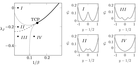
Figure 13: (a) Phase diagram for the system in the soft device at $t=0$. Parameters: $\lambda_{f}=1$, $v_{0}=0$. The transition between the Phases I and IV is continuous (bold solid line) down to the tricritical point TCP, where it becomes first-order (dashed line). The dotted lines are spinodal boundaries. The different phases are illustrated in the right column where we show the dependence of the partial free energy $\mathcal{G}$ on the internal variable $y$.

The parametric behavior of the marginal free energy $\mathcal{G}(\beta,y,t)$ in the stall conditions $t=0$ is illustrated in Fig. 13. We again observe the same four major regimes, I, II, III and IV, which have the same meaning as in the case of hard device ensemble. However, the location of the boundary between phases and the position of the tricritical point are now different, see Fig. 13(a). In Phase III, we observe that the phase minimizing Gibbs free energy is antiferromagnetic with pre- and post-power stroke conformations of cross-bridges finely interdigitated (see below). We also see that in this phase, the macroscopically homogeneous configuration stabilizes the stall state corresponding to the minimum (rather than maximum) of the energy.

As in the hard device ensemble, the parameter $\lambda_{J}$ plays the major role in the behavior of the system, which we illustrate by showing in Fig. 14 the equilibrium free energy and the force–elongation relation. One can see that in Phases I and II, the stall state is represented by the macroscopic mixture of two pure states with all cross-bridges occupying coherently either pre- or post-power stroke configuration. Instead, in Phases III and IV, the stall state is homogeneous, and cross-bridges in different conformations are microscopically mixed. The difference again is that in Phase IV, each cross-bridge is fluctuating independently between two conformational states, while in Phase III, neighboring cross-bridges are always in different conformations that are fixed in time.

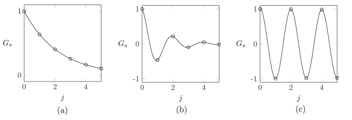
Figure 14: The equilibrium free (Gibbs) energy–strain relation in the soft device and the corresponding tension–strain relation. (a) Phase I: $\lambda_{J}=0$, $\beta=50$; (b) Phase II: $\lambda_{J}=-0.2$, $\beta=50$; (c) Phase III: $\lambda_{J}=-0.4$, $\beta=50$; and (d) Phase IV: $\lambda_{J}=-0.2$, $\beta=4$. Other parameters: $v_{0}=0$. Solid curves correspond to ground states, and dotted lines show some other stable and unstable equilibria.

Similarly to the case of the hard device, we can analytically find the location of the line of critical points separating Phases I and IV and determine the position of the tricritical point, see Fig. 13(a). To define the order parameter in the soft device case, we observe that the equilibrium of the system with respect to the variable $y$ implies $y=t+N^{-1}\sum_{i}x_{i}.$ It is then natural to define the order parameter again as $\phi=2\left<x\right>+1$, which in the soft device case gives, $\phi=2y+1-t.$

We again assume, for simplicity, $v_{0}=0$ and focus on the stall state $t=0$. We can then write the partial Gibbs free energy in the form

$$\mathcal{G}(\beta,\phi)=\frac{1}{8}+\frac{\phi^{2}}{8}-\frac{1}{\beta}\log\left[\cosh\frac{\beta\phi}{4}+\sqrt{e^{-\beta\lambda_{J}}+\sinh^{2}\frac{\beta\phi}{4}}\right].$$ (24)

The corresponding self-consistency relation defining the equilibrium value of the order parameter reads,

$$\phi_{*}=\frac{\sinh\frac{\beta\phi_{*}}{4}}{\sqrt{e^{-\beta\lambda_{J}}+\sinh^{2}\frac{\beta\phi_{*}}{4}}}.$$ (25)

Near the second-order phase transition, we can expand the free energy $\mathcal{G}$ for small $\phi$ in Taylor series. Leaving only the first terms, we obtain $\tilde{\mathcal{G}}(\beta,\phi)=a_{0}+a_{2}\phi^{2}+a_{4}\phi^{4}$ where

$$a_{0}=\frac{1}{8}-\frac{\log\left(\sqrt{e^{-\beta\lambda_{J}}}+1\right)}{\beta},a_{2}=\frac{1}{8}-\frac{\beta}{32\sqrt{e^{-\beta\lambda_{J}}}},a_{4}=\frac{\beta^{3}\left(3e^{\beta\lambda_{J}}-1\right)}{6144\sqrt{e^{-\beta\lambda_{J}}}}.$$ (26a)

The critical inverse temperature, $\beta_{c}$, is such that the second-order term in the expansion vanishes, and hence, it must solve the equation $32\sqrt{e^{-\beta_{c}\lambda_{J}}}=8\beta_{c}.$ In the limit case, where $\lambda_{J}\rightarrow 0$, we obtain $\beta_{c}=4$ which agrees with the corresponding expression in the hard device ensemble when $\lambda_{f}=0$.

To locate the tricritical point (TCP), we need to extend our Landau-type expansion to the the sixth-order. We obtain $\tilde{\mathcal{G}}(\beta,\phi)=a_{0}+a_{2}\phi^{2}+a_{4}\phi^{4}+a_{6}\phi^{6}$ where the new coefficient is

$$a_{6}=\frac{\beta^{5}\left(30e^{\beta\lambda_{J}}-45e^{2\beta\lambda_{J}}-1\right)}{2949120\sqrt{e^{-\beta\lambda_{J}}}}.$$ (27)

Putting to zero the second and the fourth term in this expansion, we obtain two equations $\beta=4e^{-\beta\lambda_{J}/2}$ and $e^{-\beta\lambda_{J}/2}=\sqrt{3}$. The tricritical point (TCP) is then located at $\beta_{TCP}=4\sqrt{3}$ and $\lambda_{JTCP}=-\log 3/4\sqrt{3}$. The first-order transition line is obtained by requiring that $\mathcal{G}(\beta,\phi=0)=\mathcal{G}(\beta,\phi=\phi_{*})$, where

$$\phi_{*}=\pm\sqrt{\frac{-a_{4}+\sqrt{a_{4}^{2}-3a_{2}a_{6}}}{3a_{6}}},$$ (28)

We can now build the full phase diagram in the 3D space $(\lambda_{J},\lambda_{f},\beta)$. Phase III and IV with $\phi=0$ can be then shown separated from Phases I and II where $\phi\neq 0$, see Fig. 15. We assume that the system is in the stall state which means $z=z_{0}$ in the hard device and $t=0$ in the soft device ensemble.

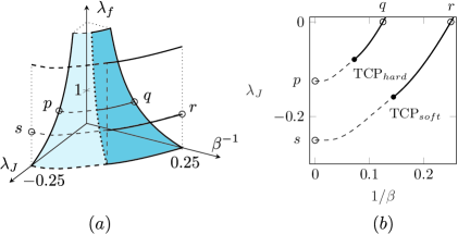
Figure 15: (a) Phase diagram in the 3D space $(\lambda_{J},\lambda_{f},\beta^{-1})$ for the case of hard device (colored surface, dark blue—second-order phase transition, light blue—first-order phase transition). The soft device phase diagram is shown by a transparent vertical cylindrical surface (b) section of both phase diagrams in (a). For the case of a hard device, we fixed the value of parameter $\lambda_{f}=1$.

In the phase diagram in Fig. 15(a), the plane $\lambda_{f}=0$ describes the soft device ensemble, while any other plane $\lambda_{f}=\text{const}>0$ corresponds to ensembles with different rigidities of the hard device. The (blue) surface separates the domain of stability of Phases III and IV from the domain of stability of Phases I and II. In this representation, the phase boundary evolves with rigidity $\lambda_{f}$ producing one parametric family of ensembles. A comparison of the sections $\lambda_{f}=0$ (soft) and $\lambda_{f}=1$ (typical hard) is presented in Fig. 15 (b) showing, for instance, that the location of the tricritical points in these two ensembles is different. Since for each half-sarcomere, the value of the lump elasticity $\lambda_{f}$ may vary with perpetual re-configuring of the surrounding effective matrix, the location of the actual tricritical point can be considered as floating.

The presence, in the phase diagram of the system, of the two closely located critical lines that terminate in the two tricritical points may contribute to the system’s ability to perform robustly and might be, in this sense, functional. Previously we have shown that such double criticality may actualize in the system of muscle cross-bridges due to quenched disorder BRT_PRL_2019 . Here, we neglect the quenched disorder, which, of course, also contributes to the destabilization of the coherent response and focus instead on steric antiferromagnetic interaction as the main factor preventing strongly cooperative response. The importance of the fact that the near-criticality condition is achieved in both soft and hard device ensembles almost concomitantly stems from the mixed nature of the loading conditions experienced by a single half-sarcomere. We recall that muscle architecture involves both parallel and series connections. Parallel elements respond to a common displacement (hard device, Helmholtz ensemble), while series structures sense a common force (soft device, Gibbs ensemble). The dominance of long-range interactions induces different collective behavior in force- and length-controlled ensembles, and to ensure the robustness of the response under a broad range of mechanical stimuli, the system can benefit from being poised in the vicinity of both types of critical regimes.

Note also that throughout this paper, we have been assuming that the stiffness $\lambda_{f}=\kappa_{f}/N$ is a size-independent constant. Therefore, we implicitly assumed that $\kappa_{f}\sim N$. We recall that the (macroscopic) stiffness $\kappa_{f}$ represents elastic filaments which support a parallel bundle of $N$ cross-bridges. An alternative assumption would be that filaments are not stiffer than cross-bridges and therefore $\kappa_{f}$ is $N$ independent, see, for instance, BRT_PRL_2019 . In this case, $\lambda_{f}\sim 1/N$, and the number of cross-bridges $N$ becomes a control parameter in the phase diagram. This means that an active control of the number of attached myosin heads could induce a structural change in the overall mechanical response of the system. For instance, it was shown that the fraction of myosin motors attached in the OFF state (heads folded back toward the M-line) depends on the thick filament stress Linari_Nature_2015 . The time course of the change in conformation of the population of myosin motors in a half-sarcomere was also traced by quick freezing of a single muscle fiber and by using cryo-EM Taylor_Cell_1999 . Such modulation of the number of attached cross-bridges may be an indication of an active control; however, the theoretical exploration of this idea will not be pursued in this paper.

6 Antiferromagnetic order

Note that the order parameter $\phi$, which is the mechanical analog of magnetization, cannot differentiate between Phases I and II when $\phi\neq 0$ and III and IV when $\phi=0$. Finer features of the local spin distribution can be captured if we introduce parameter distinguishing between ferromagnetic and antiferromagnetic spins’ arrangements.

We recall that in magnetism, the system is antiferromagnetic if it is energetically favorable for neighboring spins to align in opposite directions. In the simplest antiferromagnets, the crystal may be divided into two sublattices, A and B, so that if the spins occupying one sublattice point one way, those occupying the other point the opposite way so that the spins of nearest-neighbor atoms are always antiparallel crangle2012solid ; Zvyagin_LTP_2006 . Since the net magnetization is equal to zero in such a state, the order parameter $\phi$ cannot distinguish between paramagnetic (our Phase IV) and antiferromagnetic (our Phase III) phases.

To obtain an approximate picture of the transition to antiferromagnetic behavior, we employ a two-sublattice mean-field approximation Nagle_JAP_1971 ; Agra_2006 ; Nishino_PRB_2016 . We first introduce the conventional spin variable $s_{i}=2x_{i}+1$, so that $s_{i}=\pm 1$, and then distinguish magnetizations in different sublattices introducing $\phi_{a}=\left<s_{i\in A}\right>=(2/N)\sum_{i\in A}s_{i},$ and $\phi_{b}=\left<sz_{i\in B}\right>=(2/N)\sum_{i\in B}s_{i}.$ Then, the staggered magnetization can be defined as $\phi_{s}=(\phi_{a}-\phi_{b})/2,$ while $\phi=(\phi_{a}+\phi_{b})/2$.

If we express the Hamiltonian (7) in terms of the spin variables, $s_{i}=\pm 1$, the relaxed energy can be written as,

$$\begin{split}E(s_{i},z)=-\frac{1}{8N(1+\lambda_{f})}\sum_{i,j}s_{i}s_{j}-\frac{\lambda_{J}}{4}\sum_{i}s_{i}s_{i+1}-h(z)\sum_{i}s_{i}+f(z).\end{split}$$ (29)

where

$$h(z)=\frac{2\lambda_{f}z-1}{4(1+\lambda_{f})}+\frac{1}{4}-\frac{v_{0}}{2}+\frac{\lambda_{J}}{2},\,\,f(z)=\sum_{i}\frac{\lambda_{f}z(1+z)}{2(1+\lambda_{f})}+\frac{1}{4}+\frac{v_{0}}{2}-\frac{1}{8(1+\lambda_{f})}+\frac{\lambda_{J}}{4}.$$

This energy can be subdivided into two lattices (A and B), and in the mean-field approximation, we can express the values of spins on the corresponding sublattices as $\phi_{a,b}+\tilde{s}_{i\in A,B}$, where $\phi_{a,b}$ are the average values and the fluctuations $\tilde{s}_{i\in A,B}$ are considered to be small. Then, we obtain the approximate Hamiltonian

$$\begin{split}\mathcal{H}_{mf}&=-\frac{1}{8N(1+\lambda_{f})}\sum_{i,j}(\phi_{a}+\tilde{s}_{i\in A}+\phi_{b}+\tilde{s}_{i\in B})(\phi_{a}+\tilde{s}_{j\in A}+\phi_{b}+\tilde{s}_{j\in B})\\ &-\frac{\lambda_{J}}{4}\sum_{<i,j>}(\phi_{a}+\tilde{s}_{i\in A}+\phi_{b}+\tilde{s}_{i\in B})(\phi_{a}+\tilde{s}_{j\in A}+\phi_{b}+\tilde{s}_{j\in B})\\ &-h(z)\sum_{i\in A}(\phi_{a}+\tilde{s}_{i\in A})-h(z)\sum_{i\in B}(\phi_{b}+\tilde{s}_{i\in B})+f(z),\end{split}$$ (30)

where the notation $<i,j>$ indicates that $i$ and $j$ are nearest neighbors. We neglect quadratic terms in the fluctuation, and then, the problem is posed for $s_{i\in A,B}$, by substituting $\tilde{s}_{i\in A,B}=s_{i\in A.B}-\phi_{a,b}$,

$$\mathcal{H}_{mf}=NJ_{eff}\phi_{a}\phi_{b}+h_{a}(z)\sum_{i\in A}s_{i}+h_{b}(z)\sum_{i\in B}s_{i}+c(z),$$ (31)

where

$$J_{eff}=\frac{1}{4}\left(\frac{1}{\lambda_{f}+1}+2\lambda_{J}\right)$$

is the effective (mean-field) coupling, which depends on both short- and long-range interactions. The loading-dependent effective fields are $h_{a}(z)=-\phi_{b}J_{eff}-h_{s}(z)$ and $h_{b}(z)=-\phi_{a}J_{eff}-h_{s}(z)$, with

$$h_{s}(z)=\frac{2\lambda_{f}z-1}{4(1+\lambda_{f})}+\frac{1}{4}-\frac{v_{0}}{2}+\frac{\lambda_{J}}{2}.$$

Finally, the additive constant is $c(z)=\frac{N\lambda_{f}z^{2}}{2(1+\lambda_{f})}+Nv_{0}$. Using the self-consistency conditions $\phi_{a,b}=<\sum_{i\in{A,B}}s_{i}>$, we obtain the nonlinear algebraic equations for $\phi_{a,b}$:

$$\begin{split}\phi_{a}=\frac{1}{\mathcal{Z}_{mf}}\sum_{\{s_{i}\}}s_{i\in A}e^{-\beta\mathcal{H}_{m}f}=\tanh\beta(J_{eff}\phi_{b}+h_{s})\\ \phi_{b}=\frac{1}{\mathcal{Z}_{mf}}\sum_{\{s_{i}\}}s_{i\in B}e^{-\beta\mathcal{H}_{m}f}=\tanh\beta(J_{eff}\phi_{a}+h_{s})\end{split}$$ (32)

where $\mathcal{Z}_{mf}=2^{N}e^{-N\beta J_{eff}\phi_{a}\phi_{b}}\left(\cosh\beta h_{a}\cosh\beta h_{b}\right)^{N/2}.$ The system (32) has a unique solution $\phi_{a}=\phi_{b}=0$ for $\beta\leq\beta_{N}=-1/J_{eff}$ and acquires two additional nonzero solutions for $\beta>\beta_{N}$. The analog of stall state in this mean-field problem is $z=z_{0}^{s}=(1+1/\lambda_{f})(v_{0}-\lambda_{J})-1/2$. The phase diagram at $z=z_{0}^{s}$ is presented in Fig. 16 where we set for simplicity that $v_{0}=0$ and $\lambda_{f}=1$.

Figure 16: (a) Phase diagram of a model mean-field system in a hard device showing the boundary separating domains with different patterning of spins (representing pre- and post-power stroke configurations of the myosin heads). In the paramagnetic (PM) domain, spins are disordered; in the antiferromagnetic (AFM) domain, spins are ordered (interdigitated). The loading parameter is fixed at $z=z_{0}^{s}$. (b) Staggered magnetization $\phi_{s}$ as a function of the non-dimensional temperature $1/\beta$. (c) Order parameters for the AFM phase $\phi_{a,b}$ as functions of $1/\beta$. Other parameters: $\lambda_{J}=-0.5$.

Since we neglected the crucial long-range interactions in our system due to myosin backbones and treated the steric short-range interactions only at the mean-field level, the resulting phase diagram in Fig. 16(a) is too oversimplified to capture our four Phases I, II, III and IV. The only division which can be illustrated in this way is between the paramagnetic (PM) Phase IV and antiferromagnetic (AFM) Phase III. The corresponding line on the plane $(\lambda_{J},1/\beta)$ clearly shows that the AFM phase is favored by low temperatures and strong negativity of the coupling constant $\lambda_{J}$.

To reveal the antiferromagnetic ordering emerging in Phases II and III, we can also characterize the two-point correlation function directly $G(i,i+j)=\left<x_{i}x_{j}\right>-\left<x_{i}\right>\left<x_{j}\right>$ in the hard device ensemble by using again the transfer matrix method. Following goldenfeld1992lectures , we write

$$\begin{split}\left<x_{i}\right>=&\frac{1}{\mathcal{Z}}\int\,dy\sum_{\{x\}}e^{-\beta E(x_{i},y,z)}\,x_{i}=\frac{1}{\mathcal{Z}}\int\,dye^{-N\beta\varphi(y,z)}\sum_{x_{i}}\cdots\sum_{x_{N}}\left[\bm{T}_{x_{1}x_{2}}\bm{T}_{x_{2}x_{3}}\cdots\bm{T}_{x_{i-1}x_{i}}x_{i}\,\bm{T}_{x_{i}x_{i+1}}\cdots\right]\end{split}$$ (33)

Note that the matrix $\sum_{x_{i}}\bm{T}_{x_{i-1}x_{i}}x_{i}\,\bm{T}_{x_{i}x_{i+1}}$ can be equivalently written as $\bm{A}=\bm{T}\bm{X}\bm{T}$, where $\bm{X}=\left(\begin{array}[]{cc}0&0\\ 0&-1\end{array}\right)$ and therefore $\left<x_{i}\right>=\frac{1}{\mathcal{Z}}\int\,dy\,e^{-N\beta\varphi(y,z)}\operatorname{Tr}(\bm{X}\bm{T}^{N}).$ However, $\bm{T}=\bm{S}\bm{T^{\prime}}\bm{S}^{-1}$, where $\bm{T^{\prime}}$ is a diagonal matrix with eigenvalues, given by Eq. (11). Then, $\left<x_{i}\right>=\frac{1}{\mathcal{Z}}\int\,dy\,e^{-N\beta\varphi(y,z)}\operatorname{Tr}[\bm{S}^{-1}\bm{X}\,\bm{S}\,(\bm{T^{\prime}})^{N}].$ We can explicitly compute the eigenvectors of $\bm{T}$, $V_{\pm}=(\alpha_{\pm},1)$, where $\alpha_{\pm}=e^{\frac{\beta J}{2}}[-\sinh h\pm\sqrt{e^{-\beta J}+\sinh^{2}h}]$, so $\bm{S}=\left(\begin{array}[]{cc}\alpha_{+}&\alpha_{-}\\ 1&1\end{array}\right)$, and

$$\bm{S}^{-1}\bm{X}\,\bm{S}=\left(\begin{array}[]{cc}\chi_{11}&\chi_{12}\\ \chi_{22}&\chi_{22}\end{array}\right)\equiv\left(\begin{array}[]{cc}-\frac{\sinh h}{2\sqrt{\sinh^{2}h+e^{-\beta J}}}-\frac{1}{2}&\frac{e^{-\frac{\beta J}{2}}}{2\sqrt{\sinh^{2}h+e^{-\beta J}}}\\ \frac{e^{-\frac{\beta J}{2}}}{2\sqrt{\sinh^{2}h+e^{-\beta J}}}&\frac{\sinh h}{2\sqrt{\sinh^{2}h+e^{-\beta J}}}-\frac{1}{2}\end{array}\right).$$ (34)

Then, using Laplace method and the fact that $\lim_{N\to\infty}(\lambda_{2}/\lambda_{1})^{N}\to 0$, we obtain

$$\left<x_{i}\right>=\chi_{11}=-\frac{\sinh h}{2\sqrt{\sinh^{2}h+e^{-\beta J}}}-\frac{1}{2}.$$ (35)

The two-point correlation function can be compute similarly. Note first that

$$\begin{split}\left<x_{i}x_{j}\right>=\frac{1}{\mathcal{Z}}&\int\,dy\,e^{-N\beta\varphi(y,z)}\operatorname{Tr}\left[\bm{(}{S}^{-1}\bm{X}\,\bm{S})\,(\bm{T^{\prime}})^{j}(\bm{S}^{-1}\bm{X}\,\bm{S})\,(\bm{T^{\prime}})^{N-j}\right]\end{split}$$ (36)

Again, in the limit $N\to\infty$, we obtain $\left<x_{i}x_{j}\right>=\chi_{11}^{2}+\chi_{12}\chi_{21}\left(\lambda_{2}/\lambda_{1}\right)^{j},$ which allows us to finally write

$$G(i,i+j)=\left<x_{i}x_{j}\right>-\left<x_{i}\right>\left<x_{j}\right>=\chi_{12}\chi_{21}\left(\frac{\lambda_{2}}{\lambda_{1}}\right)^{j}=\frac{1}{4+4\,e^{\beta J}\sinh^{2}h}\left[\frac{\cosh h-\sqrt{e^{-\beta J}+\sinh^{2}h}}{\cosh h+\sqrt{e^{-\beta J}+\sinh^{2}h}}\right]^{j}.$$ (37)

Here, $h=\frac{\beta}{2}(y_{*}+1/2-v_{0})$, and $y_{*}$ is given by (14). To illustrate (37), it is convenient to use the spin variables $s_{i}=\pm 1$ defined by $2x_{i}=s_{i}-1$. In Fig. 17, we show the function $G_{s}(j)\equiv G_{s_{i}}(i,i+j)=4\,G_{x_{i}}(i,i+j)$ which clearly distinguished between the ferromagnetic (FM) and antiferromagnetic (AFM) phases; note that we do not attempt here to directly associate these regimes with the phases defined in Fig. 10.

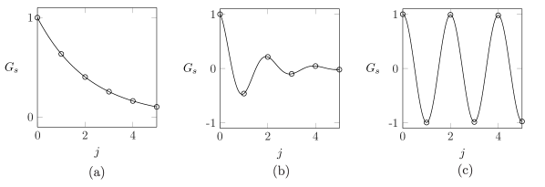
Figure 17: Two-point correlation function in different phases for the model system, see Fig. 16(a). The loading parameter is fixed at $z=z_{0}$. Other parameters: (a) $\beta=20$, $\lambda_{J}=0.1$ PM-phase; (b) $\beta=10$, $\lambda_{J}=-0.2$ PM-phase; and (c) $\beta=20$, $\lambda_{J}=-0.5$ AFM-phase.

To summarize, we have shown if short-range steric interactions between cross-bridges of antiferromagnetic type are sufficiently strong, then the state of isometric contractions is not only mechanically stable in the sense that it has positive stiffness, but it is also ordered in the way that exactly half of the cross-bridges is in pre-power stroke state and another half in the post-power stroke state; moreover, the conformation states oscillate at lattice scale so that both confirmations are effectively present at any location inside a half-sarcomere.

7 Two half-sarcomeres

In this section, we show how the presence of antiferromagnetic short-range interactions allows the system to avoid instability developing into macroscopic inhomogeneity. One can say that to maintain homogeneity at the macroscale, such system chooses to be maximally inhomogeneous at the microscopic scale.

So far, we have been dealing with a single half-sarcomere behavior, which is the basic unit of contraction. Even having non-convex elastic energy and negative stiffness, such a unit is still stable in a hard device. This case’s instability comes when more than one element with non-convex energies is loaded in a hard device while being arranged in series. Even if the system includes only two units like this, they do not need to deform in an affine way and can accept instead different deformational states.

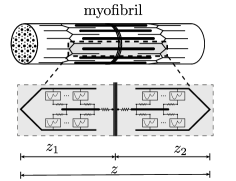
Figure 18: Schematic representation of a single sarcomere. Inset illustrates the equivalent mechanical model: two half-sarcomeres connected in series.

This is an important issue since muscle fiber is often represented as a series of connections of half-sarcomeres. It has been shown that if the energy of individual half-sarcomeres is non-convex, such association breaks into macroscopic islands of either fully pre- or fully post-power stroked half-sarcomeres Puglisi2000 ; Vilfan_BioPhys_2003 . Such instability would be prevented if the energy of a half-sarcomere is convexified in the stall configuration. As we have shown in the previous sections, such convexification occurs when the system is either in Phase IV or Phase III. It has been already known to Huxley that the first option is not viable in view of insufficiently high reduced temperature in physiological conditions. That is why we consider below the only low-temperature option when the destabilizing steric short-range interactions are sufficiently strong, and the physiological system is in Phase III.

To illustrate the disappearance of the macroscopic instability in this case, it is sufficient to consider the simplest system with only two half-sarcomeres connected in series. Such system can be viewed as a prototypical description of a single sarcomere, see Fig. 18. Experiments suggest that in stall conditions, each sarcomere contains a macroscopically (but not necessarily microscopically) uniform mixture of pre- and post-power stroke cross-bridges MIDDE20111024 .

Suppose that each half-sarcomere is equilibrated independently at the microscale and therefore behaves at the macroscale according to the elastic constitutive relation generated by the free energy $\mathcal{F}(\beta,z)$, see (13). We can then write the equilibrium energy of the whole system loaded in a hard device in the form

$$\mathcal{F}_{2}(\beta,z,z_{1})=\mathcal{F}(\beta,z_{1})+\mathcal{F}(\beta,z-z_{1}).$$ (38)

where $z$ is the macroscopic controlling parameter. The extra variable $z_{1}$ can be eliminated using the equilibrium condition $\partial\mathcal{F}(\beta,z_{1})/\partial z_{1}=\partial\mathcal{F}(\beta,z-z_{1})/\partial z_{1}$. Substituting the equilibrium value $z_{1}(\beta,z)$ into (38), we obtain the function $\mathcal{F}_{2}(\beta,z)=\mathcal{F}_{2}(\beta,z,z_{1}(\beta,z,))$ and construct the equilibrium force–elongation relation $t(\beta,z)=d\mathcal{F}_{2}(\beta,z)/dz$. It would be also of interest to compute for each half-sarcomere, the fraction of cross-bridges in either pre- or post-power stroke conformations. For half-sarcomeres 1 and 2, respectively, it will be given by the functions

$$\phi_{1,2}(\beta,z)=2(\lambda_{f}+1)y_{*}^{1,2}(\beta,z)-2\lambda_{f}z+1$$ (39)

where the function $y_{*}(\beta,z)$ is given by (14).

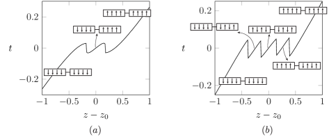
Figure 19: Mechanical response of the system consisting of two half-sarcomere units connected in series with each half-sarcomere represented by infinite number of cross-bridges (thermodynamic limit). Solid curves show the equilibrium tension–elongation curves; the insets illustrate the associated configurations of cross-bridges. Parameters: (a) $v_{0}=0$, $\beta=5$, $\lambda_{f}=1$ and $\lambda_{J}=0$ (no short-range interactions). (b) $v_{0}=0$, $\beta=25$, $\lambda_{f}=1$ and $\lambda_{J}=-0.25$ (strong antiferromagnetic short-range interactions).

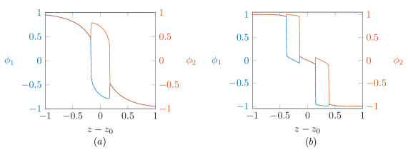
Figure 20: Strain response of the ’local’ order parameters for the system of two half-sarcomeres connected in series. The colored curves show $\phi_{1}$ and $\phi_{2}$ are the order parameter of the individual half-sarcomeres. Parameters: (a): $v_{0}=0$, $\beta=5$, $\lambda_{f}=1$ and $\lambda_{J}=0$ (no short-range interactions); b) $v_{0}=0$, $\beta=25$, $\lambda_{f}=1$ and $\lambda_{J}=-0.25$ (strong antiferromagnetic short-range interactions).

In Fig. 19 and Fig. 20, we compare the response of two half-sarcomeres in series depending on whether their constitutive response follows the one from Phase I, see Fig. 19(a) or Phase III, see Fig. 19(b).

If short-range interactions are of ferromagnetic type, and the individual subsystems are in Phase I, we observe that while the effective stiffness in the stall state $z=z_{0}$ is positive, see Fig. 19(a), the macro-state is non-affine with $\phi_{1}$ and $\phi_{2}$ taking different values. This means that the two half-sarcomeres in series have different internal structures that are both pure: One is fully in pre-power stroke state, and another one is fully in post-power stroke state, see Fig. 20(a).

If instead, the short-range interactions are of antiferromagnetic type and the individual half-sarcomeres are in Phase III, the whole sarcomere (in stall conditions) has positive stiffness, see Fig. 19(b), and its macro-configuration is affine with the order parameters $\phi_{1}$ and $\phi_{2}$ taking the same value, see Fig. 20(b). This means that the two half-sarcomeres in series have the same internal structure, which is, however, micro-inhomogeneous, with cross-bridges equally divided between pre- and post-power stroke conformations.

Outside a neighborhood of the stall state, the system with ferromagnetic-type short-range interactions is microscopically homogeneous with all half-sarcomeres occupying the same pure state. Instead, the system with antiferromagnetic-type interactions develops two zones of non-affine behavior where one of the two half-sarcomeres is in a pure state, while the other one is in a mixed state.

This simplified description can be immediately extended to cover the case of $N$ half-sarcomeres connected in series. In the case of dominating antiferromagnetic interactions, the stall state will remain mechanically stable, macroscopically homogeneous and microscopically inhomogeneous. Outside the stall state’s immediate vicinity, there will be different regimes with a variable number of coexisting half-sarcomeres in a pure and mixed state. The overall macroscopic force–elongation curve will then be wavy with an overall slightly positive average slope as observed in experiments. In the limit $N\to\infty$, we obtain weak convergence to an apparently stress–strain curve whose local microscopic derivative is nevertheless different from its macroscopic (averaged) value.

8 Conclusions

We presented a mathematical model describing the passive mechanical response of tetanized muscle fibers. It is relevant for analyzing experiments involving fast mechanical perturbations imposed on the state of isometric contractions. The observed overall homogeneity of the macroscopic response in these conditions was previously shown to contradict the microscopic prediction of the classical HS model and its more recent generalizations CT_ROPP_2018 . According to this model the slope of the force–length curve should be negative and the cross-bridges inside single half-sarcomeres must be necessarily either all in pre- or all in post-power stroke states.

The standard HS-type model assumes that the bi-stable nature of myosin heads can be modeled by spin variables and that inside a single half-sarcomere, the myosin cross-bridges are arranged in parallel Irving02 ; Higushi_Nature2017 . This parallel structure is responsible for mean-field-type interaction among different cross-bridges, which forces them to act synchronously. To compromise the coherent response of such parallel bundles, we proposed to move beyond the HS framework CAT_PRL and introduce into the model the antiferromagnetic mechanical interactions between neighboring cross-bridges. We then studied the competition between these destabilizing short-range interactions and the stabilizing long-range interactions of HS.

We showed that while an increase in the strength of the ferromagnetic short-range interactions ($\lambda_{J}>0$) would have the same effect as a decrease in temperature, leaving the overall qualitative behavior of HS unchanged, the presence of antiferromagnetic interactions ($\lambda_{J}<0$) drastically changes the qualitative behavior of the system. The main effect is that by tuning the parameter $\lambda_{J}<0$, one can introduce a new energy well corresponding to the stall state and, in this way, stabilize the state of isometric contractions. At a fixed strength of long-range interactions (fixed $\lambda_{f}$), the phase diagram in $(\beta,\lambda_{J})$ space shows a line of second-order phase transition which expands the critical regime found in CAT_PRL at $\lambda_{J}=0$.

The proposed model shows that to make a macroscopically homogeneous response possible, the system must be microscopically inhomogeneous. Micro-inhomogeneity, achieved by activating short-range interactions of antiferromagnetic type, takes the form of periodic interdigitated patterns with neighboring sarcomeres taking alternatively either pre- or post-power stroke conformations. Such patterns replace the highly coherent micro-homogeneous mechanical response favored by the original HS model. The predicted micro-inhomogeneity may be beneficial as it breaks the coherency of the response and facilitates the swift transition to either fully pre- or fully post-power stroke configuration in response to external excitation. We also argue that evolution could use short-range interactions to tune the muscle machinery to perform near the conditions of ’double criticality’, where both the Helmholtz and the Gibbs free energies are singular. Such design would be highly functional given that elementary force-producing units usually perform in a mixed soft–hard loading conditions.

We have shown that the proposed hypothesis of the ’interacting neighbors’ questions the stability of the uniform equilibrium (micro)configurations of half-sarcomeres only in the case when they respond to the mechanical perturbation analyzed in the classical HS paper. More theoretical studies are needed to evaluate how it would also affect the general kinetic response of muscle myofibrils in both passive and active phases. Another challenge is to assess how the micro-inhomogeneous nature of the response would influence the ability of the motors to use the chemical energy of the ATP. In the HS type models, this energy can be linked to the value of $v_{0}$, which may be then affected by the presence of short-range interactions. Yet another important factor to be included in future studies is the complex 3D arrangements of myosin fibers and the presence of an elaborate 3D architecture linking individual cross-bridges not only through thick and thin filaments but also, effectively, through M- and Z-disks. Only by surviving such more realistic tests in fully comprehensive settings can the hypothesis of antiferromagnetic short-range interaction gain acceptance in the muscle mechanics community.

9 Acknowledgments

The authors thank Marco Linari and Matthieu Caruel for helpful discussion. H.B.R. was supported by a PhD fellowship from Ecole Polytechnique; L. T. was supported by the grant ANR-10-IDEX-0001-02 PSL.

References

- (1) Matthieu Caruel and Lev Truskinovsky. Physics of muscle contraction. Reports on Progress in Physics, 81(3):036602, 2018.
- (2) Terrell L. Hill. Theoretical formalism for the sliding filament model of contraction of striated muscle part i. Progress in Biophysics and Molecular Biology, 28:267 – 340, 1974.
- (3) A. F. Huxley and R. M. Simmons. Proposed mechanism of force generation in striated muscle. Nature, 233(5321):533–538, 10 1971.
- (4) R. J. Podolsky. Kinetics of Muscular Contraction : the Approach to the Steady State. Nature, 188:666–668, November 1960.
- (5) Gabriella Piazzesi, Massimo Reconditi, Marco Linari, Leonardo Lucii, Yin-Biao Sun, Theyencheri Narayanan, Peter Boesecke, Vincenzo Lombardi, and Malcolm Irving. Mechanism of force generation by myosin heads in skeletal muscle. Nature, 415(6872):659–662, 02 2002.
- (6) G Piazzesi, M Reconditi, M Linari, L Lucii, P Bianco, E Brunello, V Decostre, A Stewart, DB Gore, TC Irving, M Irving, and V Lombardi. Skeletal muscle performance determined by modulation of number of myosin motors rather than motor force or stroke size. Cell, 131(4):784 – 795, 11 2007.
- (7) Malcolm Irving, Vincenzo Lombardi, Gabriella Piazzesi, and Michael A. Ferenczi. Myosin head movements are synchronous with the elementary force-generating process in muscle. Nature, 357(6374):156–158, 05 1992.
- (8) Raman Sheshka and Lev Truskinovsky. Power-Stroke-Driven Muscle Contraction, pages 117–207. Springer International Publishing, Cham, 2020.
- (9) L. Marcucci and L. Truskinovsky. Mechanics of the power stroke in myosin ii. Phys. Rev. E, 81:051915, May 2010.
- (10) L. Marcucci and L. Truskinovsky. Muscle contraction: A mechanical perspective. The European Physical Journal E, 32(4):411–418, 2010.
- (11) M. Caruel and L. Truskinovsky. Statistical mechanics of the huxley-simmons model. Phys. Rev. E, 93:062407, Jun 2016.
- (12) M. Caruel, J.-M. Allain, and L. Truskinovsky. Mechanics of collective unfolding. Journal of the Mechanics and Physics of Solids, 76:237 – 259, 2015.
- (13) Elisabetta Brunello, Marco Caremani, Luca Melli, Marco Linari, Manuel Fernandez-Martinez, Theyencheri Narayanan, Malcolm Irving, Gabriella Piazzesi, Vincenzo Lombardi, and Massimo Reconditi. The contributions of filaments and cross-bridges to sarcomere compliance in skeletal muscle. The Journal of Physiology, 592(17):3881–3899, 2014.
- (14) Marco Linari, Ian Dobbie, Massimo Reconditi, Natalia Koubassova, Malcolm Irving, Gabriella Piazzesi, and Vincenzo Lombardi. The stiffness of skeletal muscle in isometric contraction and rigor: The fraction of myosin heads bound to actin. Biophysical Journal, 74(5):2459 – 2473, 1998.
- (15) A. F. Huxley and S. Tideswell. Filament compliance and tension transients in muscle. Journal of Muscle Research & Cell Motility, 17(4):507–511, 1996.
- (16) Andrej Vilfan and Thomas Duke. Instabilities in the transient response of muscle. Biophysical journal, 85(2):818–827, 08 2003.
- (17) Matthieu Caruel, J-M Allain, and Lev Truskinovsky. Muscle as a metamaterial operating near a critical point. Physical Review Letters, 110(24):248103, 2013.
- (18) Hudson Borja da Rocha. Collective effects in muscle contraction and cellular adhesion. Theses, Université Paris-Saclay, September 2018.
- (19) A. F. Huxley. Mechanics and models of the myosin motor. Philosophical Transactions of the Royal Society B: Biological Sciences, 355(1396):433–440, 2000.
- (20) L E Ford, A F Huxley, and R M Simmons. The relation between stiffness and filament overlap in stimulated frog muscle fibres. The Journal of physiology, 311:219–249, feb 1981.
- (21) Elisabetta Brunello, Massimo Reconditi, Ravikrishnan Elangovan, Marco Linari, Yin Biao Sun, Theyencheri Narayanan, Pierre Panine, Gabriella Piazzesi, Malcolm Irving, and Vincenzo Lombardi. Skeletal muscle resists stretch by rapid binding of the second motor domain of myosin to actin. Proceedings of the National Academy of Sciences of the United States of America, 104(50):20114–20119, 2007.
- (22) G. Puglisi and Lev Truskinovsky. Mechanics of a discrete chain with bi-stable elements. Journal of the Mechanics and Physics of Solids, 48(1):1–27, 2000.
- (23) Dilson E. Rassier and Ivan Pavlov. Contractile Characteristics of Sarcomeres Arranged in Series or Mechanically Isolated from Myofibrils, pages 123–140. Springer New York, New York, NY, 2010.
- (24) Shenping Wu, Jun Liu, Mary C Reedy, Robert J Perz-Edwards, Richard T Tregear, Hanspeter Winkler, Clara Franzini-Armstrong, Hiroyuki Sasaki, Carmen Lucaveche, Yale E Goldman, Michael K Reedy, and Kenneth A Taylor. Structural changes in isometrically contracting insect flight muscle trapped following a mechanical perturbation. PloS one, 7(6):e39422–e39422, 2012.
- (25) Richard T. Tregear, Mary C. Reedy, Yale E. Goldman, Kenneth A. Taylor, Hanspeter Winkler, Clara Franzini-Armstrong, Hiroyuki Sasaki, Carmen Lucaveche, and Michael K. Reedy. Cross-bridge number, position, and angle in target zones of cryofixed isometrically active insect flight muscle. Biophysical Journal, 86(5):3009 – 3019, 2004.
- (26) Massimo Reconditi. Recent improvements in small angle x-ray diffraction for the study of muscle physiology. Reports on Progress in Physics, 69(10):2709–2759, 2006.
- (27) R T Tregear, R J Edwards, T C Irving, K J Poole, M C Reedy, H Schmitz, E Towns-Andrews, and M K Reedy. X-ray diffraction indicates that active cross-bridges bind to actin target zones in insect flight muscle. Biophysical Journal, 74(3):1439–1451, 03 1998.
- (28) G. Piazzesi and V. Lombardi. A cross-bridge model that is able to explain mechanical and energetic properties of shortening muscle. Biophysical Journal, 68(5):1966–1979, 1995.
- (29) D. A. Smith, M. A. Geeves, J. Sleep, and S. M. Mijailovich. Towards a unified theory of muscle contraction. i: Foundations. Annals of Biomedical Engineering, 36(10):1624–1640, 2008.
- (30) D. A. Smith and S. M. Mijailovich. Toward a unified theory of muscle contraction. ii: Predictions with the mean-field approximation. Annals of Biomedical Engineering, 36(8):1353, 2008.
- (31) Marco Caremani, Luca Melli, Mario Dolfi, Vincenzo Lombardi, and Marco Linari. Force and number of myosin motors during muscle shortening and the coupling with the release of the atp hydrolysis products. The Journal of Physiology, 593(15):3313–3332, 2015.
- (32) Hudson Borja da Rocha and Lev Truskinovsky. Functionality of disorder in muscle mechanics. Phys. Rev. Lett., 122:088103, Mar 2019.
- (33) R. Sheshka, P. Recho, and L. Truskinovsky. Rigidity generation by nonthermal fluctuations. Phys. Rev. E, 93:052604, May 2016.
- (34) John F. Nagle. Ising chain with competing interactions. Phys. Rev. A, 2:2124–2128, Nov 1970.
- (35) J. C. Bonner and J. F. Nagle. Phase behavior of models with competing interactions. Journal of Applied Physics, 42(4):1280–1282, 1971.
- (36) Mehran Kardar. Crossover to equivalent-neighbor multicritical behavior in arbitrary dimensions. Phys. Rev. B, 28:244–246, Jul 1983.
- (37) Per Arne Rikvold, Gregory Brown, Seiji Miyashita, Conor Omand, and Masamichi Nishino. Equilibrium, metastability, and hysteresis in a model spin-crossover material with nearest-neighbor antiferromagnetic-like and long-range ferromagnetic-like interactions. Phys. Rev. B, 93:064109, Feb 2016.
- (38) Alessandro Campa, Giacomo Gori, Vahan Hovhannisyan, Stefano Ruffo, and Andrea Trombettoni. Ising chains with competing interactions in the presence of long-range couplings. Journal of Physics A: Mathematical and Theoretical, 52(34):344002, jul 2019.
- (39) Freddy Bouchet, Shamik Gupta, and David Mukamel. Thermodynamics and dynamics of systems with long-range interactions. Physica A: Statistical Mechanics and its Applications, 389(20):4389 – 4405, 2010. Proceedings of the 12th International Summer School on Fundamental Problems in Statistical Physics.
- (40) Julien Barré, David Mukamel, and Stefano Ruffo. Inequivalence of ensembles in a system with long-range interactions. Phys. Rev. Lett., 87:030601, Jun 2001.
- (41) Julien Barré, David Mukamel, and Stefano Ruffo. Ensemble Inequivalence in Mean-Field Models of Magnetism, pages 45–67. Springer Berlin Heidelberg, Berlin, Heidelberg, 2002.
- (42) Lorenzo Marcucci, Takumi Washio, and Toshio Yanagida. Including Thermal Fluctuations in Actomyosin Stable States Increases the Predicted Force per Motor and Macroscopic Efficiency in Muscle Modelling. PLoS Computational Biology, 12(9):1–20, 2016.
- (43) Massimo Ostilli and Farrukh Mukhamedov. 1D Three-state mean-field Potts model with first- and second-order phase transitions. Physica A, 555:124415, 2020.
- (44) J.M. Yeomans. Statistical Mechanics of Phase Transitions. Clarendon Press, 1992.
- (45) John M. Squire, Danielle M. Paul, and Edward P. Morris. Myosin and Actin Filaments in Muscle: Structures and Interactions, pages 319–371. Springer International Publishing, Cham, 2017.
- (46) Motoshi Kaya, Yoshiaki Tani, Takumi Washio, Toshiaki Hisada, and Hideo Higuchi. Coordinated force generation of skeletal myosins in myofilaments through motor coupling. Nature Communications, 8:16036, 2017.
- (47) Maria V. Razumova, Anna E. Bukatina, and Kenneth B. Campbell. Different myofilament nearest-neighbor interactions have distinctive effects on contractile behavior. Biophysical Journal, 78(6):3120 – 3137, 2000.
- (48) John M. Squire. Muscle myosin filaments: cores, crowns and couplings. Biophysical Reviews, 1(3):149, 2009.
- (49) Alf Månsson, Dilson Rassier, and Georgios Tsiavaliaris. Poorly Understood Aspects of Striated Muscle Contraction. BioMed Research International, 2015:245154, 2015.
- (50) Bertrand C. W Tanner, Thomas L Daniel, and Michael Regnier. Sarcomere lattice geometry influences cooperative myosin binding in muscle. PLOS Computational Biology, 3(7):1–17, 07 2007.
- (51) Kanji Oshima, Yasunori Takezawa, Yasunobu Sugimoto, Takakazu Kobayashi, Thomas C. Irving, and Katsuzo Wakabayashi. Axial dispositions and conformations of myosin crossbridges along thick filaments in relaxed and contracting states of vertebrate striated muscles by x-ray fiber diffraction. Journal of Molecular Biology, 367(1):275–301, 2007.
- (52) T L Hill, E Eisenberg, and L Greene. Theoretical model for the cooperative equilibrium binding of myosin subfragment 1 to the actin-troponin-tropomyosin complex. Proceedings of the National Academy of Sciences, 77(6):3186–3190, 1980.
- (53) William O Hancock, Lee L Huntsman, and Albert M Gordon. Models of calcium activation account for differences between skeletal and cardiac force redevelopment kinetics. Journal of Muscle Research & Cell Motility, 18(6):671–681, 1997.
- (54) John Jeremy Rice, Gustavo Stolovitzky, Yuhai Tu, and Pieter P. de Tombe. Ising model of cardiac thin filament activation with nearest-neighbor cooperative interactions. Biophysical Journal, 84(2):897 – 909, 2003.
- (55) Srboljub M. Mijailovich, Jeffrey J. Fredberg, and James P. Butler. On the theory of muscle contraction: Filament extensibility and the development of isometric force and stiffness. Biophysical Journal, 71(3):1475–1484, 1996.
- (56) Thomas L. Daniel, Alan C. Trimble, and P. Bryant Chase. Compliant realignment of binding sites in muscle: Transient behavior and mechanical tuning. Biophysical Journal, 74(4):1611–1621, 1998.
- (57) P Bryant Chase, J Michael Macpherson, and Thomas L Daniel. A Spatially Explicit Nanomechanical Model of the Half-Sarcomere: Myofilament Compliance Affects Ca2+-Activation. Annals of Biomedical Engineering, 32(11):1559–1568, 2004.
- (58) Kenneth S. Campbell. Filament compliance effects can explain tension overshoots during force development. Biophysical Journal, 91(11):4102–4109, 2006.
- (59) Joseph D. Powers, Pasquale Bianco, Irene Pertici, Massimo Reconditi, Vincenzo Lombardi, and Gabriella Piazzesi. Contracting striated muscle has a dynamic i-band spring with an undamped stiffness 100 times larger than the passive stiffness. The Journal of Physiology, 598(2):331–345, 2020.
- (60) Pierre-Gilles de Gennes. Maximum pull out force on dna hybrids. Comptes Rendus de l’Académie des Sciences - Series IV - Physics, 2(10):1505–1508, 2001.
- (61) Xiaofeng Ren and Lev Truskinovsky. Finite Scale Microstructures in Nonlocal Elasticity. Journal of elasticity and the physical science of solids, 59(1):319–355, 2000.
- (62) Paul M Chaikin, Tom C Lubensky, and Thomas A Witten. Principles of condensed matter physics, volume 10. Cambridge university press Cambridge, 1995.
- (63) K. Midde, R. Luchowski, H.K. Das, J. Fedorick, V. Dumka, I. Gryczynski, Z. Gryczynski, and J. Borejdo. Evidence for pre- and post-power stroke of cross-bridges of contracting skeletal myofibrils. Biophysical Journal, 100(4):1024 – 1033, 2011.
- (64) Keiko Hirose and Takeyuki Wakabayashi. Structural change of crossbridges of rabbit skeletal muscle during isometric contraction. Journal of Muscle Research & Cell Motility, 14(4):432–445, 1993.
- (65) M.C. Reedy. Visualizing myosin’s power stroke in muscle contraction. Journal of Cell Science, 113(20):3551–3562, 2000.
- (66) D D Thomas, S Ramachandran, O Roopnarine, D W Hayden, and E M Ostap. The mechanism of force generation in myosin: a disorder-to-order transition, coupled to internal structural changes. Biophysical journal, 68(4 Suppl):135S–141S, apr 1995.
- (67) Massimo Reconditi, Marco Caremani, Francesca Pinzauti, Joseph D. Powers, Theyencheri Narayanan, Ger J. M. Stienen, Marco Linari, Vincenzo Lombardi, and Gabriella Piazzesi. Myosin filament activation in the heart is tuned to the mechanical task. Proceedings of the National Academy of Sciences, 114(12):3240–3245, 2017.
- (68) G Piazzesi, F Francini, M Linari, and V Lombardi. Tension transients during steady lengthening of tetanized muscle fibres of the frog. The Journal of physiology, 445:659–711, jan 1992.
- (69) Massimo Reconditi, Marco Linari, Leonardo Lucii, Alex Stewart, Yin-Biao Sun, Peter Boesecke, Theyencheri Narayanan, Robert F Fischetti, Tom Irving, Gabriella Piazzesi, Malcolm Irving, and Vincenzo Lombardi. The myosin motor in muscle generates a smaller and slower working stroke at higher load. Nature, 428(6982):578–581, 2004.
- (70) N. Goldenfeld. Lectures on phase transitions and the renormalization group. Frontiers in physics. Addison-Wesley, Advanced Book Program, 1992.
- (71) Kim Christensen and Nicholas R Moloney. Complexity and criticality, volume 1. World Scientific Publishing Company, 2005.
- (72) R.K. Pathria and P.D. Beale. Statistical Mechanics. Elsevier Science, 1996.
- (73) Alessandro Campa, Thierry Dauxois, and Stefano Ruffo. Statistical mechanics and dynamics of solvable models with long-range interactions. Physics Reports, 480(3-6):57–159, 2009.
- (74) Marco Linari, Elisabetta Brunello, Massimo Reconditi, Luca Fusi, Marco Caremani, Theyencheri Narayanan, Gabriella Piazzesi, Vincenzo Lombardi, and Malcolm Irving. Force generation by skeletal muscle is controlled by mechanosensing in myosin filaments. Nature, 528(7581):276–279, 2015.
- (75) Kenneth A Taylor, Holger Schmitz, Mary C Reedy, Yale E Goldman, Clara Franzini-Armstrong, Hiroyuki Sasaki, Richard T Tregear, Kate Poole, Carmen Lucaveche, Robert J Edwards, Li Fan Chen, Hanspeter Winkler, and Michael K Reedy. Tomographic 3D Reconstruction of Quick-Frozen, Ca<sup>2+</sup>-Activated Contracting Insect Flight Muscle. Cell, 99(4):421–431, nov 1999.
- (76) John Crangle. Solid· State Magnetism. Springer Science & Business Media, 2012.
- (77) A. A. Zvyagin and G. A. Skorobagat’ko. On the mean-field theory of a two-sublattice antiferromagnet. Low Temperature Physics, 32(7):644–649, 2006.
- (78) Rafael Agra, Frédéric van Wijland, and Emmanuel Trizac. On the free energy within the mean-field approximation. European Journal of Physics, 27(2):407–412, feb 2006.
- (79) Malcolm Irving, Gabriella Piazzesi, Leonardo Lucii, Yin-Biao Sun, Jeffrey J Harford, Ian M Dobbie, Michael A Ferenczi, Massimo Reconditi, and Vincenzo Lombardi. Conformation of the myosin motor during force generation in skeletal muscle. Nature Structural Biology, 7(6):482–485, 2000.