Implementing contact angle boundary conditions for second-order Phase-Field models of wall-bounded multiphase flows

Abstract

In the present work, a general formulation is proposed to implement the contact angle boundary conditions for the second-order Phase-Field models, which is applicable to $N$-phase $(N\geqslant 2)$ moving contact line problems. To remedy the issue of mass change due to the contact angle boundary condition, a source term or Lagrange multiplier is added to the original second-order Phase-Field models, which is determined by the consistent and conservative volume distribution algorithm so that the summation of the order parameters and the consistency of reduction are not influenced. To physically couple the proposed formulation to the hydrodynamics, especially for large-density-ratio problems, the consistent formulation is employed. The reduction-consistent conservative Allen-Cahn models are chosen as examples to illustrate the application of the proposed formulation. The numerical scheme that preserves the consistency and conservation of the proposed formulation is employed to demonstrate its effectiveness. Results produced by the proposed formulation are in good agreement with the exact and/or asymptotic solutions. The proposed method captures complex dynamics of moving contact line problems having large density ratios.

Keywords: Contact angle; Contact line; Phase-Field; Allen-Cahn; Conservative Phase-Field; Multiphase flow

1 Introduction

Moving contact line problems are ubiquitous in both natural phenomena and industrial applications. Various numerical models have been developed for this kind of problems, such as the front tracking method (UnverdiTryggvason1992, ; Tryggvasonetal2001, ; ManservisiScardovelli2009, ; MuradogluTasoglu2010, ), the level-set method (OsherSethian1988, ; SethianSmereka2003, ; Spelt2005, ; ZhangYue2020, ), the conservative level-set method (OlssonKreiss2005, ; Olssonetal2007, ; Zahedietal2009, ; Satoetal2012, ), and the volume-of-fluid (VOF) method (HirtNichols1981, ; ScardovelliZaleski1999, ; Renardyetal2001, ; Afkhamietal2009, ; Yokoi2011, ), and the contact angle boundary conditions therein. We refer interested readers to the comprehensive review (Suietal2014, ).

In the present study, we focus on the Phase-Field (or Diffuse-Interface) models (Andersonetal1998, ), where the interface is represented as a transient layer with a small but finite thickness. Different from the sharp-interface models, which only include advection, diffusion in the Phase-Field models regularizes the singularity at the contact line. Such an additional effect can drive the contact line to move even though the no-slip boundary condition is assigned (Seppecher1996, ; Jacqmin2000, ). One commonly used procedure to derive the contact angle boundary conditions for the Phase-Field models is in the context of wall energy relaxation (Jacqmin2000, ; Qianetal2006, ; Dong2012, ; Baietal2017a, ; Shenetal2020, ), where the wall energy is minimized by the $L^{2}$ gradient flow. Such a procedure has been extended to include surfactant (Zhuetal2020, ), contact angle hysteresis (Yue2020, ), three fluid phases (ShiWang2014, ; Shenetal2015, ; ZhangWang2016, ), and $N$ ($N\geqslant 2$) fluid phases (Dong2017, ). Alternatively, the contact angle boundary conditions can also be geometry-based (DingSpelt2007, ; LeeKim2011, ; Loudetetal2020, ), where the orientation of the interface is explicitly enforced, and the one in (DingSpelt2007, ) has been extended to model contact lines formed by three fluid phases (Zhangetal2016, ). Most of these contact angle boundary conditions can be in general written as an inhomogeneous Neumann boundary condition. Among various Phase-Field models, the Cahn-Hilliard Phase-Field model (CahnHilliard1958, ) is most popularly used to model moving contact line problems, since the contact angle boundary conditions can be directly applied without influencing the mass conservation. The Cahn-Hilliard model is a 4th-order partial differential equation (PDE) and therefore we also call it a 4th-order Phase-Field model here. To uniquely solve it, each boundary requires two boundary conditions, one of which is determined by mass conservation. Flexibility is given to the remaining one to control the morphology of the interface, which is achieved by implementing the contact angle boundary conditions. The popularity of implementing the Cahn-Hilliard model has motivated several theoretical analyses, e.g., in (Jacqmin2000, ; Qianetal2006, ; Yueetal2010, ; YueFeng2011, ; Xuetal2018, ), and comparison studies, e.g., in (DingSpelt2007, ; Lacisetal2020, ).

More recently, the second-order Phase-Field models, such as the conservative Phase-Field models (ChiuLin2011, ; Mirjalilietal2020, ) and the conservative Allen-Cahn models (BrasselBretin2011, ; Huangetal2020B, ), have attracted lots of attention and became popular in modeling both two-phase flows, e.g., in (ChiuLin2011, ; MirjaliliMani2021, ; JeongKim2017, ; JoshiJaiman2018, ; JoshiJaiman2018adapt, ; Huangetal2020CAC, ), and $N$-phase ($N\geqslant 2$) flows, e.g., in (Aiharaetal2019, ; Huetal2020, ; Huangetal2020B, ). They are modified from the Allen-Cahn model (AllenCahn1979, ) and enjoy several desirable properties that the Cahn-Hilliard model does not have, but are important in multiphase flow modeling, such as conserving volume enclosed by the interface, preserving under-resolved structures, and the maximum principle (BrasselBretin2011, ; Kimetal2014, ; LeeKim2016, ; KimLee2017, ; Chaietal2018, ; Mirjalilietal2020, ; Huangetal2020CAC, ; Huangetal2020B, ). Moreover, it is easier and more efficient to solve the 2nd-order model than the 4th-order one. However, difficulty appears when these 2nd-order Phase-Field models are used to model problems including moving contact lines, because only a single boundary condition is needed. This boundary condition is always determined by the mass conservation and the homogeneous Neumann boundary condition is normally required. Consequently, only $90^{0}$ contact angle can be assigned at the wall boundary, which strongly restricts the application of the second-order Phase-Field models. So far, the second-order Phase-Field models have not been able to share the fruitful progress made in the implementation of the contact angle boundary conditions for moving contact line problems.

The present study attempts to address this issue and proposes a novel and general formulation which has the following desirable properties:

• It is valid for both two-phase and $N$-phase ($N>2$) cases.

• It does not rely on the specific forms of the 2nd-order Phase-Field models and the contact angle boundary conditions.

• It grantees the consistency of reduction, the mass conservation of each phase, and the summation of the volume fractions to be unity.

• It incorporates the consistency of mass conservation and the consistency of mass and momentum transport for large-density-ratio problems.

The idea is to introduce a Lagrange multiplier to the original Phase-Field model, so that the mass change due to the contact angle boundary condition is compensated. The Lagrange multiplier needs to be carefully designed to avoid producing voids, overfilling, or fictitious phases, and therefore the consistent and conservative volume distribution algorithm is employed (Huangetal2020B, ). Finally, the coupling to the hydrodynamics is accomplished by using the consistent formulation (Huangetal2020CAC, ), which is essential for large-density-ratio problems. This general formulation is applied to the reduction-consistent conservative Allen-Cahn models (Brackbilletal1992, ; Huangetal2020B, ), and various tests are performed to demonstrate its effectiveness.

The consistency of reduction, consistency of mass conservation, and consistency of mass and momentum transport are modeling principles followed in the present study. The consistency of reduction (BoyerMinjeaud2014, ; Dong2017, ; Dong2018, ; Huangetal2020B, ) requires that a $N$-phase model should be able to reduce to the corresponding $M$-phase ($1\leqslant M\leqslant N-1$) model when ($N-M$) phases are absent. Fictitious phases can be produced if this principle is violated, as demonstrated in the references mentioned. The consistency of mass conservation and consistency of mass and momentum transport (Huangetal2020, ; Huangetal2020CAC, ; Huangetal2020N, ) illustrate the mass and momentum transport in the Phase-Field models, which couples the Phase-Field models to the hydrodynamics. Violating these principles can produce density-ratio-dependent velocity fluctuations, as demonstrated in the references mentioned. These consistency conditions have been successfully implemented to not only two/$N$-phase flows (Huangetal2020, ; Huangetal2020CAC, ; Huangetal2020N, ; Huangetal2020B, ) but also multiphase flows with mass transfer (Huangetal2020NPMC, ) and solidification/melting (Huangetal2021Solid, ). Various problems having density ratios beyond $1,000$ have been tested in those references. We refer interested readers to (Dong2018, ; Huangetal2020, ; Huangetal2020N, ) where the definitions and analyses of the consistency conditions are detailed.

The rest of the paper is organized as follows. In Section 2, the general formulation to include the contact angle boundary condition in the second-order Phase-Field models and its coupling to the hydrodynamics are elaborated, followed by its application to the conservative Allen-Cahn models. In Section 3, the numerical methods to solve the complete system is briefly summarized. In Section 4, various numerical tests are performed to demonstrate the proposed formulation in moving contact line problems. In Section 5, the present study is concluded and some possible future directions are introduced.

2 Definitions and governing equations

We first define the problem in Section 2.1. Then, the general formulation of implementing the contact angle boundary condition for a second-order Phase-Field model is proposed and elaborated in Section 2.2.1, along with its coupling to the hydrodynamics in Sections 2.2.2 and 2.2.3. Finally, two specific examples, one for two-phase problems and the other for $N$-phase problems, are provided in Section 2.3, which are the applications of the proposed general formulation described in Section 2.2.1 to the conservative Allen-Cahn models.

2.1 Basic definitions

There are $N$ ($N\geqslant 2$) different incompressible and immiscible fluid phases inside domain $\Omega$, and their locations are labeled by a set of order parameters $\{\phi_{p}\}_{p=1}^{N}$. The order parameters need to follow the summation constraint:

$$\sum_{p=1}^{N}C_{p}=\sum_{p=1}^{N}\frac{1+\phi_{p}}{2}=1\quad\mathrm{or}\quad\sum_{p=1}^{N}\phi_{p}=2-N,$$ (1)

where $\{C_{p}\}_{p=1}^{N}$ are the volume fractions of the phases and therefore their summation is always unity. In other words, void or overfilling is not allowed to appear. The densities and viscosities of the phases are denoted by $\{\rho_{p}\}_{p=1}^{N}$ and $\{\mu_{p}\}_{p=1}^{N}$, respectively. As a result, the mixture density and viscosity are

$$\rho=\sum_{p=1}^{N}\rho_{p}\frac{1+\phi_{p}}{2},\quad\mu=\sum_{p=1}^{N}\mu_{p}\frac{1+\phi_{p}}{2}.$$ (2)

Each pair of phases has a surface tension, for example, $\sigma_{p,q}$ denotes the surface tension at the interface of Phases $p$ and $q$. $\theta_{p,q}$ is the contact angle in between Phase $p$ and a wall boundary and formed by Phases $p$ and $q$. Notice that $\sigma_{p,q}$ ($=\sigma_{q,p}$) is symmetry, while $\theta_{p,q}$ and $\theta_{q,p}$ are supplementary angles, i.e., $\theta_{p,q}+\theta_{q,p}=\pi$, $1\leqslant p,q\leqslant N$. Since each phase is incompressible, the flow velocity is divergence-free (Abelsetal2012, ; Dong2018, ; Huangetal2020N, ), i.e.,

$$\nabla\cdot\mathbf{u}=0.$$ (3)

If there are only two phases, we denote $\phi_{1}=\phi$, $\phi_{2}=-\phi$, $\sigma=\sigma_{1,2}$, and $\theta=\theta_{1,2}$ for convenience. Consequently, one only needs to solve $\phi_{1}$ (or $\phi$), and $\phi_{2}$ is obtained automatically from Eq.(1), or equivalently $\phi_{2}=-\phi_{1}=-\phi$. Unless otherwise specified, the domain boundary $\partial\Omega$ is composed of wall boundaries, although periodic, inflow, or outflow boundaries can be incorporated, depending on specific problems.

2.2 Governing equations

The problem to be modeled by the second-order Phase-Field model and the contact angle boundary condition is sketched in Fig.1. Here, the emphasis is on answering how to implement the contact angle boundary condition in the second-order Phase-Field model with the proposed general formulation. The hydrodynamics is included, following the consistency of mass conservation and the consistency of mass and momentum transport (Huangetal2020, ; Huangetal2020CAC, ).

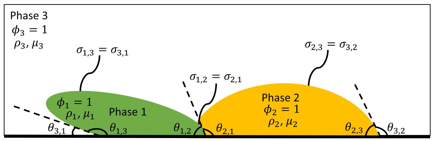
Figure 1: Sketch of the problem to be modeled by the second-order Phase-Field model and the contact angle boundary condition.

2.2.1 The proposed general formulation

The general form of the second-order Phase-Field model can be written as

$$\frac{\partial\phi_{p}}{\partial t}+\nabla\cdot(\mathbf{u}\phi_{p})=\mathcal{L}_{p}[\{\phi_{q}\}_{q=1}^{N}]\quad\mathrm{in}\quad\Omega,\quad 1\leqslant p\leqslant N,$$ (4)

where $\mathcal{L}$ represents a functional of the order parameters, and the highest (spatial) derivatives included are the second-order derivatives. This is the reason that Eq.(4) is called the second-order Phase-Field model. Because of the divergence-free velocity Eq.(3), the convection term in Eq.(4) has been written in a conservative form. To be physically admissible, $\mathcal{L}$ has the following properties:

$$\sum_{q=1}^{N}\mathcal{L}_{q}=0,\quad\int_{\Omega}\mathcal{L}_{p}d\Omega=0,\quad\mathcal{L}_{p}|_{\phi_{p}=-1}=0,\quad 1\leqslant p\leqslant N.$$ (5)

The first property in Eq.(5) comes from the summation of the order parameters Eq.(1). The second one implies the mass conservation of Phase $p$, which is shown more clearly after Eq.(4) is integrated over $\Omega$:

$$\frac{d}{dt}\int_{\Omega}\phi_{p}d\Omega+\int_{\partial\Omega}\mathbf{n}\cdot\mathbf{u}\phi_{p}d\Gamma=0,\quad 1\leqslant p\leqslant N.$$ (6)

Since $\mathcal{L}$ usually contains a diffusive term of type $\nabla^{2}\phi$, to achieve the second property in Eq.(5) and therefore the mass conservation of individual phases, i.e., Eq.(6), the homogeneous Neumann boundary condition is needed, i.e., $\int_{\Omega}\nabla^{2}\phi d\Omega=\int_{\partial\Omega}\mathbf{n}\cdot\nabla\phi d\Gamma=0$. Such a boundary condition avoids the diffusive flux into wall boundaries. Additionally with the impermeability condition, i.e., $\mathbf{n}\cdot\mathbf{u}=0$, at the domain boundary, we have $\frac{d}{dt}\int_{\Omega}\phi_{p}d\Omega=0$ from Eq.(6), which means the total mass of Phase $p$ in $\Omega$ will not change. The last property in Eq.(5) corresponds to the consistency of reduction in the sense that Phase $p$ will not be produced if it is absent, i.e., $(\partial\phi_{p}/\partial t)|_{\phi_{p}=-1}=0$. Notice that the convection term now becomes $\nabla\cdot(\mathbf{u}\phi_{p})|_{\phi_{p}=-1}=-\nabla\cdot\mathbf{u}=0$. However, in the present study, the contact angle boundary condition, i.e.,

$$\mathbf{n}\cdot\nabla\phi_{p}=\mathcal{F}_{p}^{w}[\{\phi_{q}\}_{q=1}^{N};\{\theta_{q,r}\}_{q,r=1}^{N}]\quad\mathrm{at}\quad\partial\Omega,\quad 1\leqslant p\leqslant N,$$ (7)

needs to be implemented instead of the homogeneous Neumann boundary condition. As a result, the second property of $\mathcal{L}$ in Eq.(5) is not guaranteed, and the mass conservation of each phase, i.e., Eq.(6), is probably violated. It should be noted that the notation in Eq.(7) is simplified, and $\mathcal{F}^{w}$ and $\{\theta_{p,q}\}_{p,q=1}^{N}$ can be different at individual wall boundaries in practice. Similar to $\mathcal{L}$, physically admissible $\mathcal{F}^{w}$ has the following properties:

$$\sum_{q=1}^{N}\mathcal{F}_{q}^{w}=0,\quad\mathcal{F}_{p}^{w}|_{\phi_{p}=-1}=0,\quad 1\leqslant p\leqslant N,$$ (8)

compatible with the summation of the order parameters Eq.(1) and the consistency of reduction, respectively. This can be clearly seen after summing Eq.(7) over the phases or setting $\phi_{p}=-1$ in Eq.(7), and one obtains the respective two properties in Eq.(8).

In order to implement the contact angle boundary condition Eq.(7), while other physical principles are not violated, we propose to modify the second-order Phase-Field model Eq.(4) to be

$$\frac{\partial\phi_{p}}{\partial t}+\nabla\cdot(\mathbf{u}\phi_{p})=\mathcal{L}_{p}[\{\phi_{q}\}_{q=1}^{N}]+L_{p}^{w}\quad\mathrm{in}\quad\Omega,\quad 1\leqslant p\leqslant N,$$ (9)

where $L^{w}$ is the newly introduced Lagrange multiplier and has the following properties:

$$\sum_{q=1}^{N}L_{q}^{w}=0,\quad\int_{\Omega}L_{p}^{w}d\Omega=-\int_{\Omega}\mathcal{L}_{p}d\Omega=S_{p}\quad\mathrm{with}\quad\mathbf{n}\cdot\nabla\phi_{p}=\mathcal{F}_{p}^{w}\quad\mathrm{at}\quad\partial\Omega,\quad L_{p}^{w}|_{\phi_{p}=-1}=0,$$ (10)

$$1\leqslant p\leqslant N,$$

to satisfy the summation of the order parameters Eq.(1), mass conservation of the phases Eq.(6), and consistency of reduction, as explained below Eq.(5). Here, we call $L^{w}$ a Lagrange multiplier, following studies like (shen2011, ; BrasselBretin2011, ; Kimetal2014, ; LeeKim2016, ) which calls a source term added to the Phase-Field equation to enforce mass conservation a Lagrange multiplier. Now, the question turns into determining $L^{w}$ that satisfies Eq.(10). This question is successfully addressed by the consistent and conservative volume distribution algorithm in (Huangetal2020B, ). Specifically, $L^{w}$ is determined by

$$L_{p}^{w}=\sum_{q=1}^{N}W_{p,q}B_{q}^{w},\quad 1\leqslant p\leqslant N,$$ (11)

$$\sum_{q=1}^{N}\left(\int_{\Omega}W_{p,q}d\Omega\right)B_{q}^{w}=S_{p},\quad W_{p,q}=\left\{\begin{array}[]{cc}-(1+\phi_{p})(1+\phi_{q}),&p\neq q,\\ (1+\phi_{p})(1-\phi_{q}),&p=q.\end{array}\right.$$ (14)

Notice that $B^{w}$ depends only on time and is solved from a $N$-by-$N$ symmetry and diagonally dominant linear system, thanks to the definition of $W_{p,q}$. Due to $\sum_{p=1}^{N}W_{p,q}=0$ from Eq.(1) and the definition of $W_{p,q}$ in Eq.(11), it is straightforward to show $\sum_{p=1}^{N}L_{p}^{w}=\sum_{q=1}^{N}B_{q}^{w}(\sum_{p=1}^{N}W_{p,q})=0$. Satisfying the other two properties in Eq.(10) by $L^{w}$ in Eq.(11) is obvious, and the related proofs are available in (Huangetal2020B, ). We refer interested readers to (Huangetal2020B, ) for more details and analyses of the volume distribution algorithm which determines $L^{w}$ in Eq.(11).

When there are only two phases, as shown in (Huangetal2020B, ), one can obtain $L^{w}$ from Eq.(11) explicitly, i.e.,

$$L_{p}^{w}=\frac{W_{p}}{\int_{\Omega}W_{p}d\Omega}S_{p},\quad W_{p}=1-\phi_{p}^{2},\quad p=1,2.$$ (15)

As a result, we have the following two-phase second-order Phase-Field model with the contact angle boundary condition:

$$\frac{\partial\phi}{\partial t}+\nabla\cdot(\mathbf{u}\phi)=\mathcal{L}[\phi]+L^{w}\quad\mathrm{in}\quad\Omega,\quad\mathbf{n}\cdot\nabla\phi=\mathcal{F}^{w}[\phi;\theta]\quad\mathrm{at}\quad\partial\Omega,$$ (16)

$$L^{w}=\frac{W}{\int_{\Omega}Wd\Omega}S,\quad S=-\int_{\Omega}\mathcal{L}d\Omega,\quad W=1-\phi^{2}.$$

Good performances of using $W_{p,q}$ in Eq.(11) and its two-phase reduction $W_{p}$ in Eq.(15) in Phase-Field models have been shown in previous studies, e.g., (BrasselBretin2011, ; Kimetal2014, ; LeeKim2016, ; Huangetal2020B, ). Their validity in two-/multi-phase flows has been evidenced, e.g., in (Huangetal2020CAC, ; JeongKim2017, ; JoshiJaiman2018, ; JoshiJaiman2018adapt, ; Huangetal2020B, ) where physical results are reported.

The proposed general formulation is summarized as follows: given any physically admissible second-order Phase-Field model, i.e., Eq.(4) satisfying Eq.(5), and contact angle boundary condition, i.e., Eq.(7) satisfying Eq.(8), a new second-order Phase-Field model is developed, i.e., Eq.(9) and Eq.(11), with the same contact angle boundary condition Eq.(7), so that the summation of the order parameters Eq.(1), mass conservation of the phases Eq.(6), and consistency of reduction are all satisfied. For two-phase problems, the proposed formulation becomes Eq.(16).

2.2.2 Mass conservation and consistent formulation

Before coupling to the hydrodynamics, we need to first determine the actual mass transport governed by the newly developed second-order Phase-Field model Eq.(9) and the mixture density Eq.(2). For a clear presentation, we combine $\mathcal{L}$ and $L^{w}$, i.e., $L=\mathcal{L}+L^{w}$, in Eq.(9), and obtain

$$\frac{\partial\phi_{p}}{\partial t}+\nabla\cdot(\mathbf{u}\phi_{p})=L_{p}\quad\mathrm{in}\quad\Omega,\quad 1\leqslant p\leqslant N,$$ (17)

$$\int_{\Omega}L_{p}d\Omega=0,\quad 1\leqslant p\leqslant N,$$ (18)

with the contact angle boundary condition Eq.(7). Next, we apply the consistent formulation (Huangetal2020CAC, ):

$$\nabla\cdot(W_{Q}(\phi_{p})\nabla Q_{p})=L_{p}\quad\mathrm{in}\quad\Omega,\quad\mathbf{n}\cdot\nabla Q_{p}=0\quad\mathrm{at}\quad\partial\Omega,\quad W_{Q}(\phi)=1-\phi^{2},\quad 1\leqslant p\leqslant N.$$ (19)

Here, $Q$ is the auxiliary variable of the consistent formulation. The consistent formulation Eq.(19) relates the non-local term $L$ to a local conservative form. More details about the consistent formulation are available in its original work (Huangetal2020CAC, ), and not repeated here. Notice that the homogeneous Neumann boundary condition of $Q$ is obtained from Eq.(18). After considering Eq.(17) and Eq.(19), the newly proposed Phase-Field model Eq.(9) is equivalent to

$$\frac{\partial\phi_{p}}{\partial t}+\nabla\cdot\mathbf{m}_{\phi_{p}}=0,$$ (20)

where the Phase-Field flux $\mathbf{m}_{\phi}$ is

$$\mathbf{m}_{\phi_{p}}=\mathbf{u}\phi_{p}-W_{Q}(\phi_{p})\nabla Q_{p},\quad 1\leqslant p\leqslant N.$$ (21)

Following the formulation in (Huangetal2020N, ), we can immediately obtain the consistent mass flux:

$$\mathbf{m}=\sum_{p=1}^{N}\frac{\rho_{p}}{2}(\mathbf{u}+\mathbf{m}_{\phi_{p}}),$$ (22)

which leads to the mass conservation equation:

$$\frac{\partial\rho}{\partial t}+\nabla\cdot\mathbf{m}=0,$$ (23)

after the mixture density Eq.(2) is included. The derivations in this section is based on the consistency of mass conservation proposed and analyzed in (Huangetal2020, ; Huangetal2020N, ; Huangetal2020CAC, ).

2.2.3 Momentum equation

The fluid motion is governed by the momentum equation:

$$\frac{\partial(\rho\mathbf{u})}{\partial t}+\nabla\cdot(\mathbf{m}\otimes\mathbf{u})=-\nabla P+\nabla\cdot\left[\mu(\nabla\mathbf{u}+\nabla\mathbf{u}^{T})\right]+\rho\mathbf{g}+\mathbf{f}_{s},$$ (24)

where $P$ is the pressure, $\mathbf{g}$ is the gravity, and $\mathbf{f}_{s}$ is the surface tension force. Notice that the same mass flux $\mathbf{m}$, defined in Eq.(22), appears in both the mass conservation equation Eq.(23) and the inertial term of the momentum Eq.(24), which is required by the consistency of mass and momentum transport (Huangetal2020, ; Huangetal2020CAC, ). As a result, the momentum equation Eq.(24) satisfies not only the momentum conservation but also kinetic energy conservation (neglecting the viscosity, gravity and surface tension) and Galilean invariance, see (Huangetal2020N, ). It should also be noted that simply using $\nabla\cdot(\rho\mathbf{u}\otimes\mathbf{u})$ as the nonlinear inertial term in the momentum equation cannot simultaneously achieve these physical properties .

In the present study, the surface tension force is

$$\mathbf{f}_{s}=\xi\nabla\phi,\quad\xi=\lambda\left(\frac{1}{\eta^{2}}g^{\prime}(\phi)-\nabla^{2}\phi\right),\quad\lambda=\frac{3}{2\sqrt{2}}\sigma\eta,\quad g(\phi)=\frac{1}{4}(1-\phi^{2})^{2},$$ (25)

for two-phase problems, and

$$\mathbf{f}_{s}=\frac{1}{2}\sum_{p=1}^{N}\xi_{p}\nabla\phi_{p},\quad\xi_{p}=\sum_{q=1}^{N}\lambda_{p,q}\left[\frac{1}{\eta^{2}}(g^{\prime}_{1}(\phi_{p})-g^{\prime}_{2}(\phi_{p}+\phi_{q}))+\nabla^{2}\phi_{q}\right],$$ (26)

$$\lambda_{p,q}=\frac{3}{2\sqrt{2}}\sigma_{p,q}\eta,\quad g_{1}(\phi)=\frac{1}{4}(1-\phi^{2})^{2},\quad g_{2}(\phi)=\frac{1}{4}\phi^{2}(\phi+2)^{2},$$

for multiphase problems. Here, $\lambda$ or $\lambda_{p,q}$ is the mixing energy density, $\eta$ is the interface thickness, $g(\phi)$, $g_{1}(\phi)$, and $g_{2}(\phi)$ are potential functions, and $g^{\prime}(\phi)$, $g^{\prime}_{1}(\phi)$, and $g^{\prime}_{2}(\phi)$ are their derivatives with respect to $\phi$. Eq.(25) and Eq.(26) have been widely used in two-phase and $N$-phase flows, e.g., in (Jacqmin1999, ; DongShen2012, ; Huangetal2020, ; Huangetal2020CAC, ; Dong2018, ; Huangetal2020N, ; HowardTartakovsky2020, ; Huetal2020, ).

In summary, given any physically admissible 2nd-order Phase-Field model and contact angle boundary condition, i.e., $\mathcal{L}$ and $\mathcal{F}^{w}$, the governing equations include Eq.(9) for the order parameters, Eq.(19) from the consistent formulation, and Eq.(24) and Eq.(3) for the velocity and pressure. In the governing equations, the density (viscosity), consistent mass flux, and surface tension force are computed from Eq.(2), Eq.(22), and Eq.(26) (or Eq.(25)), respectively.

The proposed formulation has not considered the second law of thermodynamics, because many popularly used 2nd-order Phase-Field models, such as (BrasselBretin2011, ; ChiuLin2011, ), and the contact angle boundary conditions, particularly the geometry-based ones and the $N$-phase ones, e.g., (DingSpelt2007, ; LeeKim2011, ; Loudetetal2020, ; Zhangetal2016, ; Dong2017, ), are not explicitly shown to be consistent with the second law of thermodynamics. Moreover, it is still an open question to obtain a Lagrange multiplier that satisfies the constraints in Eq.(10) and at the same time be consistent with the second law of thermodynamics. Actually, satisfying the constraints in Eq.(10) alone is a very challenging task. We implement the algorithm in (Huangetal2020B, ) to determine $L^{w}$ that satisfies all the constraints in Eq.(10), but we are still unclear whether it is consistent with the second law of thermodynamics. Lastly, following the analyses in (Huangetal2020N, ), we would like to point out that, as long as the Phase-Field models with the contact angle boundary conditions are consistent with the second law of thermodynamics, such consistency will still be true after adding the momentum equation Eq.(24).

2.3 Application to the conservative Allen-Cahn models

In the present study, the conservative Allen-Cahn models are considered as examples to demonstrate the effectiveness of the general formulation developed in Section 2.2.1. Specific formulations of $\mathcal{L}$ in the second-order Phase-Field model Eq.(4) and $\mathcal{F}^{w}$ in the contact angle boundary condition Eq.(7) are provided, and both two-phase and $N$-phase formulations are considered.

2.3.1 Two-Phase model

The two-phase conservative Allen-Cahn model proposed in (BrasselBretin2011, ) is considered, where $\mathcal{L}$ in the model is defined as

$$\mathcal{L}[\phi]=M\lambda\left(\nabla^{2}\phi-\frac{1}{\eta^{2}}g^{\prime}(\phi)\right)+L^{c},$$ (27)

$$L^{c}=WB^{c},\quad W=1-\phi^{2},\quad B^{c}=\frac{\int_{\Omega}\frac{M\lambda}{\eta^{2}}g^{\prime}(\phi)d\Omega}{\int_{\Omega}Wd\Omega}.$$

Here, $M$ is the mobility. One can easily show that $\mathcal{L}$ in Eq.(27) satisfies all the conditions in Eq.(5), and therefore it is physically admissible. The two-phase contact angle boundary condition considered is

$$\mathcal{F}^{w}[\phi;\theta]=\frac{\sqrt{2}}{3\eta}\cos(\theta)g^{\prime}_{w}(\phi),$$ (28)

which is proposed in (Jacqmin2000, ) from a wall functional. Here, $g_{w}(\phi)$ is an interpolation function satisfying $g_{w}(\pm 1)=\pm 1$ and $g^{\prime}_{w}(\pm 1)=0$, and we choose $g_{w}(\phi)=\sin\left(\frac{\pi}{2}\phi\right)$, like (Shenetal2015, ; Baietal2017a, ; Huangetal2020, ; Shenetal2020, ). Another choice of $g_{w}(\phi)$ is the Hermite polynomial, i.e., $g_{w}(\phi)=\frac{1}{2}\phi(3-\phi^{2})$, used, e.g., in (Jacqmin2000, ; Dong2012, ; ZhangWang2016, ; Yue2020, ). Our tests do not find distinguishable difference of these two choices. Again, $\mathcal{F}^{w}$ in Eq.(28) is physically admissible since it satisfies Eq.(8).

Then, we apply the proposed formulations in Section 2.2.1, i.e., Eq.(16), which introduces $L^{w}$ to the two-phase conservative Allen-Cahn model. Since both $L^{c}$ in Eq.(27) and $L^{w}$ in Eq.(16) share an identical weight function $W=1-\phi^{2}$, we can combine $L^{c}$ and $L^{w}$, i.e., $L^{a}=L^{c}+L^{w}$, as well as $B^{c}$ and $B^{w}$, i.e., $B=B^{c}+B^{w}$, for simplicity. As a result, we reach the following system:

$$\frac{\partial\phi}{\partial t}+\nabla\cdot(\mathbf{u}\phi)=M\lambda\left(\nabla^{2}\phi-\frac{1}{\eta^{2}}g^{\prime}(\phi)\right)+L^{a}\quad\mathrm{in}\quad\Omega,\quad\mathbf{n}\cdot\nabla\phi=\frac{\sqrt{2}}{3\eta}\cos(\theta)g^{\prime}_{w}(\phi)\quad\mathrm{at}\quad\partial\Omega,$$ (29)

$$L^{a}=WB,\quad W=1-\phi^{2},\quad B=\frac{\int_{\Omega}M\lambda\left(\frac{1}{\eta^{2}}g^{\prime}(\phi)-\nabla^{2}\phi\right)d\Omega}{\int_{\Omega}Wd\Omega},\quad g_{w}(\phi)=\sin\left(\frac{\pi}{2}\phi\right).$$

One can understand $L^{a}$ in Eq.(29) serving as a Lagrange multiplier to compensate the mass change inside $\Omega$ from $\frac{M\lambda}{\eta^{2}}g^{\prime}(\phi)$ and at $\partial\Omega$ from the contact angle boundary condition.

2.3.2 $N$-Phase model

Here, we consider the reduction-consistent multiphase conservative Allen-Cahn model proposed in (Huangetal2020B, ), where $\mathcal{L}$ is defined as

$$\mathcal{L}_{p}[\{\phi_{q}\}_{q=1}^{N}]=M\lambda_{0}\left(\nabla^{2}\phi_{p}-\frac{1}{\eta^{2}}\left(g^{\prime}(\phi_{p})-\frac{1+\phi_{p}}{2}L^{s}\right)\right)+L_{p}^{c},\quad 1\leqslant p\leqslant N,$$ (30)

$$L^{s}=\sum_{q=1}^{N}g^{\prime}(\phi_{q}),\quad L_{p}^{c}=\sum_{q=1}^{N}W_{p,q}B_{q}^{c},\quad\int_{\Omega}L_{p}^{c}d\Omega=\int_{\Omega}\frac{M\lambda_{0}}{\eta^{2}}\left(g^{\prime}(\phi_{p})-\frac{1+\phi_{p}}{2}L^{s}\right)d\Omega.$$

Here, $\lambda_{0}=\max(\lambda_{p,q})$, and $L^{c}$ is also determined from the consistent and conservative volume distribution algorithm (Huangetal2020B, ). Therefore $\mathcal{L}$ in Eq.(30) satisfies all the conditions in Eq.(5) and is physically admissible. We employ the reduction-consistent contact angle boundary condition proposed in (Dong2017, ), whose formulation is

$$\mathcal{F}_{p}^{w}[\{\phi_{q}\}_{q=1}^{N};\{\theta_{q,r}\}_{q,r=1}^{N}]=\sum_{q=1}^{N}\zeta_{p,q}\frac{1+\phi_{p}}{2}\frac{1+\phi_{q}}{2},\quad 1\leqslant p\leqslant N,$$ (31)

$$\zeta_{p,q}=\frac{2\sqrt{2}}{\eta}\cos(\theta_{p,q}).$$

Notice that $\zeta_{p,q}$ is antisymmetric, i.e., $\zeta_{p,q}=-\zeta_{q,p}$. Therefore, $\mathcal{F}^{w}$ in Eq.(31) also satisfies Eq.(8) and is physically admissible.

Similar to the two-phase case in Section 2.3.1, we combine $L^{c}$ and $L^{w}$ after applying the general formulation proposed in Section 2.2.1, i.e., Eq.(9). Therefore, we have the following system:

$$\frac{\partial\phi_{p}}{\partial t}+\nabla\cdot(\mathbf{u}\phi_{p})=M\lambda_{0}\left(\nabla^{2}\phi_{p}-\frac{1}{\eta^{2}}\left(g^{\prime}(\phi_{p})-\frac{1+\phi_{p}}{2}L^{s}\right)\right)+L_{p}^{a}\quad\mathrm{in}\quad\Omega,$$ (32)

$$\mathbf{n}\cdot\nabla\phi_{p}=\sum_{q=1}^{N}\zeta_{p,q}\frac{1+\phi_{p}}{2}\frac{1+\phi_{q}}{2}\quad\mathrm{at}\quad\partial\Omega,\quad 1\leqslant p\leqslant N,$$

$$L^{s}=\sum_{q=1}^{N}g^{\prime}(\phi_{q}),\quad L_{p}^{a}=\sum_{q=1}^{N}W_{p,q}B_{q},\quad\int_{\Omega}L_{p}^{a}d\Omega=\int_{\Omega}M\lambda_{0}\left(\frac{1}{\eta^{2}}\left(g^{\prime}(\phi_{p})-\frac{1+\phi_{p}}{2}L^{s}\right)-\nabla^{2}\phi_{p}\right)d\Omega,$$

$$W_{p,q}=\left\{\begin{array}[]{cc}-(1+\phi_{p})(1+\phi_{q}),&p\neq q,\\ (1+\phi_{p})(1-\phi_{q}),&p=q.\end{array}\right.,\quad\zeta_{p,q}=\frac{2\sqrt{2}}{\eta}\cos(\theta_{p,q}).$$ (35)

$L^{a}$ in Eq.(32) distributes the mass change due to both the Allen-Cahn model and the contact angle boundary condition consistently and conservatively, thanks to the volume distribution algorithm in (Huangetal2020B, ). Based on the analyses in (Huangetal2020B, ; Dong2017, ), Eq.(32) will exactly reduce to Eq.(29) with $g_{w}(\phi)$ the Hermite polynomial, i.e., $g_{w}(\phi)=\frac{1}{2}\phi(3-\phi^{2})$, when there are only two phases. Then, Eq.(29) or Eq.(32) is coupled to the hydrodynamics following Section 2.2.2 and Section 2.2.3.

Here, Eq.(29) and Eq.(32) are the specific forms of Eq.(9) of the proposed general formulation in Section 2.2.1, based on the conservative Allen-Cahn models. The rest of the governing equations have already been summarized at the end of Section 2.2.3.

3 Discretizations

Details of applying the consistent formulation discretely and solving the momentum equation consistently and conservatively are available in our previous works (Huangetal2020, ; Huangetal2020CAC, ). The balanced-force method (Huangetal2020, ; Huangetal2020N, ) is used to compute the surface tension force in Eq.(25) and Eq.(26). The (modified) conservative Allen-Cahn equations Eq.(29) and Eq.(32) are numerically solved from the 2nd-order schemes in (Huangetal2020CAC, ; Huangetal2020B, ), where the Allen-Cahn model, i.e., the one neglecting all the Lagrange multipliers, is first solved, and then the Lagrange multipliers are obtained from satisfying the summation of the order parameters Eq.(1), the mass conservation Eq.(18), and the consistency of reduction. All the integrals are computed using the mid-point rule. The schemes are semi-implicit based on the 2nd-order backward difference in time. The convection terms are treated explicitly with the 5th-order WENO scheme (JiangShu1996, ), and the diffusion terms are treated implicitly with the 2nd-order central difference (FerzigerPeric2001, ). The non-linear term $g^{\prime}(\phi)$ in both Eq.(29) and Eq.(32) is first linearized and then treated implicitly. More details of the schemes can be found in (Huangetal2020CAC, ; Huangetal2020B, ).

The only difference in the present study appears at the boundary condition of the order parameters, where the homogeneous Neumann boundary condition is replaced by the contact angle boundary condition. This requires only minor changes, and the contact angle boundary condition is implemented explicitly following (Huangetal2020, ; Huangetal2020N, ; Dong2012, ; Dong2017, ), i.e.,

$$\mathbf{n}\cdot\nabla\phi_{p}^{n+1}=\mathcal{F}_{p}^{w}[\{\phi_{q}^{*,n+1}\}_{q=1}^{N};\{\theta_{q,r}\}_{q,r=1}^{N}],$$ (36)

where $\phi^{*,n+1}$ is an explicit evaluation of $\phi^{n+1}$ from $\phi^{n}$, $\phi^{n-1}$ etc. Specifically, $\phi^{*,n+1}=\phi^{n}$ is the first-order estimate, i.e., $\phi^{n+1}-\phi^{*,n+1}=\phi^{n+1}-\phi^{n}\sim O(\Delta t)$, and $\phi^{*,n+1}=2\phi^{n}-\phi^{n-1}$ is the second-order estimate, i.e., $\phi^{n+1}-\phi^{*,n+1}=\phi^{n+1}-2\phi^{n}+\phi^{n-1}\sim O(\Delta t^{2})$. We use the second-order estimate in the present study.

In summary, the solution procedure is as follows:

1. Solve Eq.(32) (or Eq.(29)) with the scheme in (Huangetal2020B, ) (or (Huangetal2020CAC, )) and the boundary condition Eq.(36) to update the order parameters.

2. Solve Eq.(19) with the scheme in (Huangetal2020CAC, ) and then use Eq.(21) to obtain the Phase-Field flux.

3. Compute the density and viscosity with Eq.(2), the consistent mass flux with Eq.(22), the surface tension force in Eq.(26) (or Eq.(25)) with the balanced-force method (Huangetal2020, ; Huangetal2020N, ).

4. Solve Eq.(24) and Eq.(3) to update the velocity and pressure with the scheme in (Huangetal2020, ).

The chosen scheme has been carefully analyzed and verified, and we refer interested readers to (Huangetal2020, ; Huangetal2020N, ; Huangetal2020CAC, ; Huangetal2020B, ) for more details.

4 Results

Here, we mainly focus on demonstrating the effectiveness of the proposed general formulation in Section 2.2.1, which applies to the conservative Allen-Cahn models in Section 2.3, on modeling problems including moving contact lines. When setting up a case, it is sometimes more convenient to non-dimensionalize the governing equations in Section 2.2 and Section 2.3. Given a density scale $\rho_{\mathrm{ref}}$, length scale $L_{\mathrm{ref}}$, and acceleration scale $a_{\mathrm{ref}}$, one can determine the scales of other variables in the governing equations, and they are listed in Table 1, specifically to the conservative Allen-Cahn models. Using those scales in Table 1, one is able to obtain the dimensionless governing equations. The procedure is the same if $\rho_{\mathrm{ref}}$, $L_{\mathrm{ref}}$, and $u_{\mathrm{ref}}$ is given, and now $a_{\mathrm{ref}}$ becomes $u_{\mathrm{ref}}^{2}/L_{\mathrm{ref}}$ from Table 1.

Table 1: Scales of the variables in the conservative Allen-Cahn models given a density scale $\rho_{\mathrm{ref}}$, length scale $L_{\mathrm{ref}}$, and acceleration scale $a_{\mathrm{ref}}$

The initial velocity is $\mathbf{u}=\mathbf{0}\mathrm{m/s}$ and we set $M\lambda=10^{-3}L_{\mathrm{ref}}u_{\mathrm{ref}}$ and $\eta=h$ unless otherwise specified, where $h$ denotes the grid size.

4.1 Equilibrium drop

Here, we consider a semicircle liquid drop sliding on a horizontal solid wall using the two-phase model Eq.(29). The water drop initially has a radius of $R_{0}=8\mathrm{mm}$, and is surrounded by the air. The material properties of the water and air considered are listed in Table 2. The viscosities of the water and air are increased $20$ and $10$ times, respectively, in order to reach the equilibrium more quickly. Such a modification will not affect the conclusions drawn from the present section.

Table 2: Material properties in the equilibrium drop

Considering the inertia-capillary velocity scale from the Weber number $We=\rho_{1}U^{2}R_{0}/\sigma_{1,2}=1$, we have the Reynolds number $Re=\rho_{1}UR_{0}/\mu_{1}=38$, and capillary number $Ca=\mu_{1}U/\sigma_{1,2}=0.0263$. When the gravity is neglected, i.e., $|\mathbf{g}|=0$, one can obtain the final shape of the drop exactly using the mass conservation and the contact angle (deGennesetal2003, ). The exact solution is

$$R_{d}=R_{0}\sqrt{\frac{\pi/2}{\theta-\sin(\theta)\cos(\theta)}},\quad H_{d}=R_{d}(1-\cos(\theta)),\quad L_{d}=2R_{d}\sin(\theta),$$ (37)

where $R_{d}$, $H_{d}$, and $L_{d}$ are the final radius, height, and spreading length of the drop, respectively, and $\theta$ is the contact angle. Based on the asymptotic analysis for gravity-dominant cases (deGennesetal2003, ), the final height of the drop becomes

$$H_{d}=2\sqrt{\frac{\sigma_{ds}}{\rho_{d}|\mathbf{g}|}}\sin(\theta/2),$$ (38)

where $\rho_{d}$ is the density of the drop, $\sigma_{ds}$ is the surface tension between the drop and the surrounding phase, and $\mathbf{g}$ is the gravity pointing downward.

In the computation, we use $\rho_{2}$ (the air density), $L_{\mathrm{ref}}=5R_{0}=40\mathrm{mm}$, and $a_{\mathrm{ref}}=1\mathrm{m/s^{2}}$ as the density, length, and acceleration scales, respectively, to non-dimensionalize the governing equations. The length scale is chosen such that $\max(L_{d})/L_{\mathrm{ref}}\sim O(1)$, where $\max(L_{d})$ denotes the maximum final spreading length of the drop in all the considered cases. The acceleration scale is chosen for convenience when we investigate the effect of the gravity, as the dimensionless gravity will have the same value as the dimensional one. After the non-dimensionalization, the computational domain is $[-0.5,0.5]\times[0,0.3]$, and the drop is initially on the middle of the bottom wall. The lateral boundaries are periodic while they are no-slip walls at the top and bottom. Different contact angles are assigned at the bottom wall. We use $150\times 45$ grid cells and time step $\Delta t=1\times 10^{-4}$ to discretize the space and time, respectively. All the results in this section are presented in their dimensionless forms.

We first neglect the gravity. Fig.2 shows the evolution of the drop with $\theta=60^{0}$ and $\theta=135^{0}$, along with the corresponding exact final solution from Eq.(37). As expected, the drop starts with the semicircle shape, gradually approaches the final exact solution. The equilibrium shape agrees with the exact solution very well. We consider the zero contour of $\phi$ as the interface and measure the final height and spreading length of the drop for quantitative comparison. As shown in Fig.3 a), a good agreement with the exact solution from Eq.(37) is obtained. Note that the height of the domain is changed to $0.5$ for $\theta=135^{0}$ and $\theta=150^{0}$, while the grid size remains unchanged. To investigate the convergence with respect to grid refinement, the errors of the height and spreading length of the water drop versus the grid size is shown in Fig.4 a), using data from $\theta=60^{0}$. The observed convergence rate is between 1st- and 2nd-order. The saturated error of $L_{d}$ in Fig.4 a) can be caused by the evaluation of the spreading length. Since the distance from the bottom wall to the grid points nearest to it is a half of the grid size, the linear extrapolation is used to evaluate the interface location at the bottom wall, which introduces additional errors in the spreading length. Moreover, interactions of the Phase-Field model and the contact angle boundary condition, both of which are non-linear, are also involved at the bottom wall. These complicated factors come into play, which makes the analyses of the saturation in Fig.4 a) very difficult. Alternatively, we evaluate the time $t_{c}$ after which the kinetic energy ($E_{K}=\int_{\Omega}\frac{1}{2}\rho\mathbf{u}\cdot\mathbf{u}d\Omega$) is less than $10^{-5}$. Considering the finest-grid result as the reference value, a convergence rate near 2nd order is observed in Fig.4 b). Additionally, we supplement, in Appendix A, a manufactured solution problem, which is commonly used to demonstrate the convergence. The convergence of the order parameter, velocity, and pressure with respect to the cell size is observed.

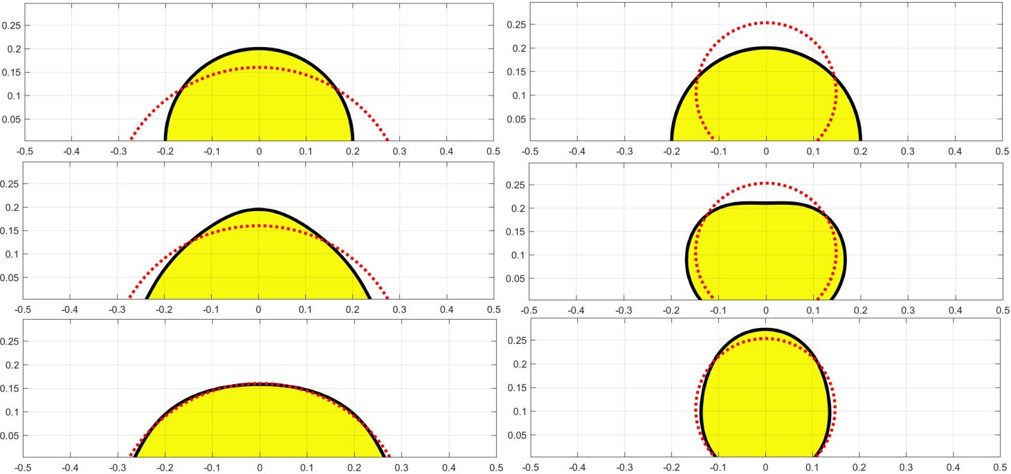
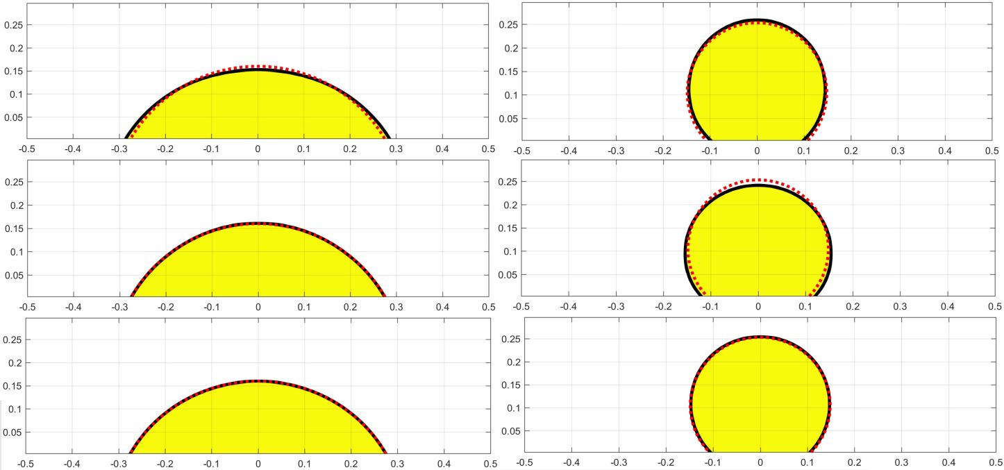
Figure 2: Evolution of the water drop using Eq.(29) with $|\mathbf{g}|=0$. Yellow: water ( Phase 1); White: air (Phase 2); Red dotted line: exact solution from Eq.(37). Left column: $\theta=60^{0}$; Right column: $\theta=135^{0}$. From top to bottom, $t=0.0$, $t=0.2$, $t=0.4$, $t=1.0$, $t=1.4$, and $t=2.0$ (left) and $t=3.0$ (right).

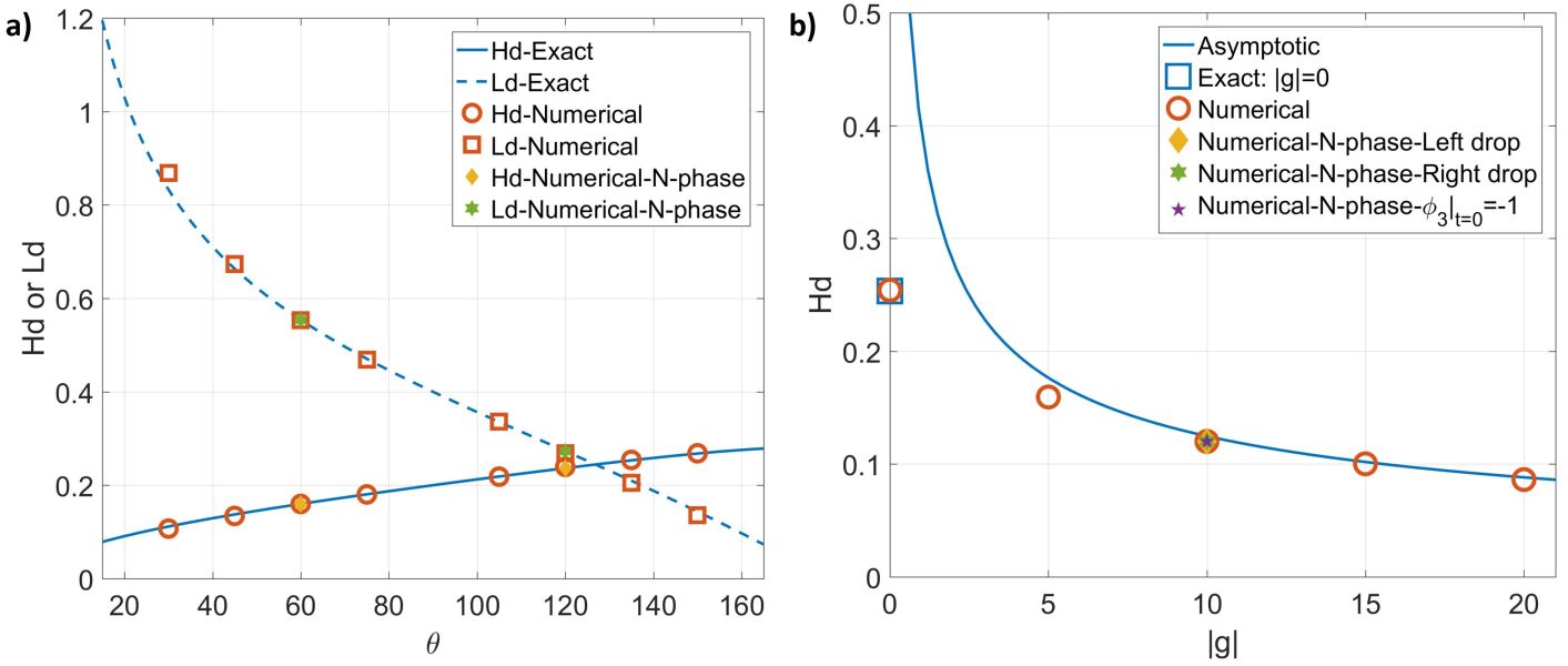
Figure 3: Height and spreading length of the drop. a) $H_{d}$ and $L_{d}$ versus $\theta$ with $|\mathbf{g}|=0$. b) $H_{d}$ versus $|\mathbf{g}|$ with $\theta=135^{0}$.

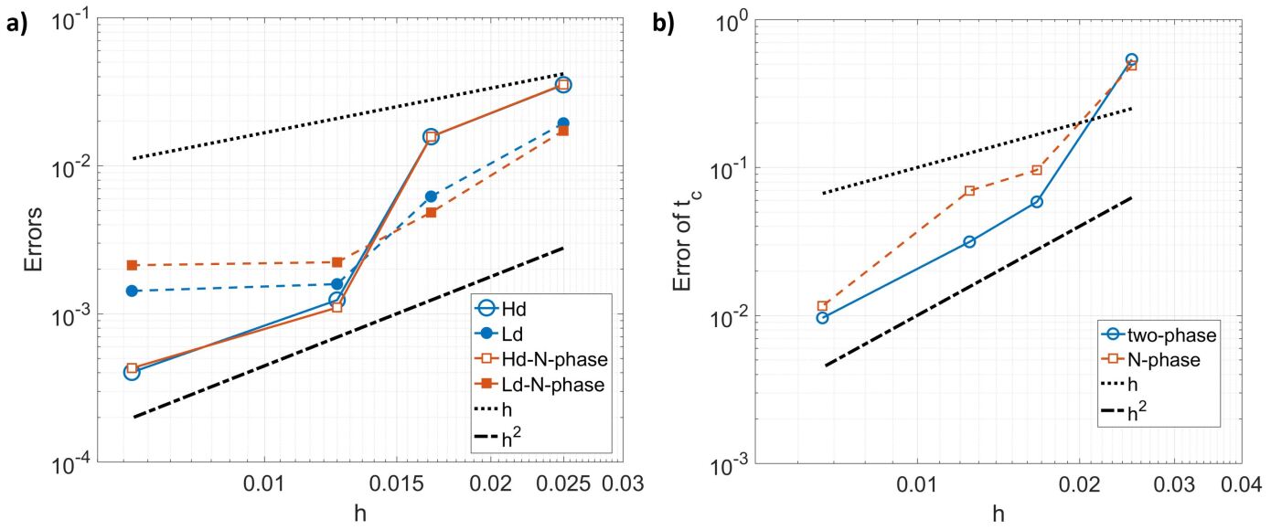
Figure 4: Convergence behaviors versus the grid size. a) Errors of the height and spreading length, and b) Errors of $t_{c}$ after which the kinetic energy ($E_{K}=\int_{\Omega}\frac{1}{2}\rho\mathbf{u}\cdot\mathbf{u}d\Omega$) is less than $10^{-5}$, from the cases of the water drop with $\theta=\theta_{1,2}=60^{0}$ and $|\mathbf{g}|=0$.

Then, the effect of gravity is included, and the domain is changed to $[-0.6,0.6]\times[0,0.24]$ without changing the grid size. Fig.5 shows the evolution of the drop with $|\mathbf{g}|=10$ and $|\mathbf{g}|=15$, along with the prediction from Eq.(38). The contact angle is $\theta=135^{0}$. One can observe that the drop is flattened, having a pancake-like shape, when the gravity is added. The final height of the drop matches the asymptotic prediction. Fig.3 b) shows the final height of the drop versus the gravity, and our numerical prediction overall agrees well with both the exact solution Eq.(37) without gravity and the asymptotic solution Eq.(38) with dominant gravity. Further, Fig.6 a) demonstrates the mass conservation of the proposed formulation, where the relative changes of $\Phi$ ($\Phi=\int_{\Omega}\phi d\Omega$) of the four cases reported in Fig.2 and Fig.5 are in the order of the round-off error.

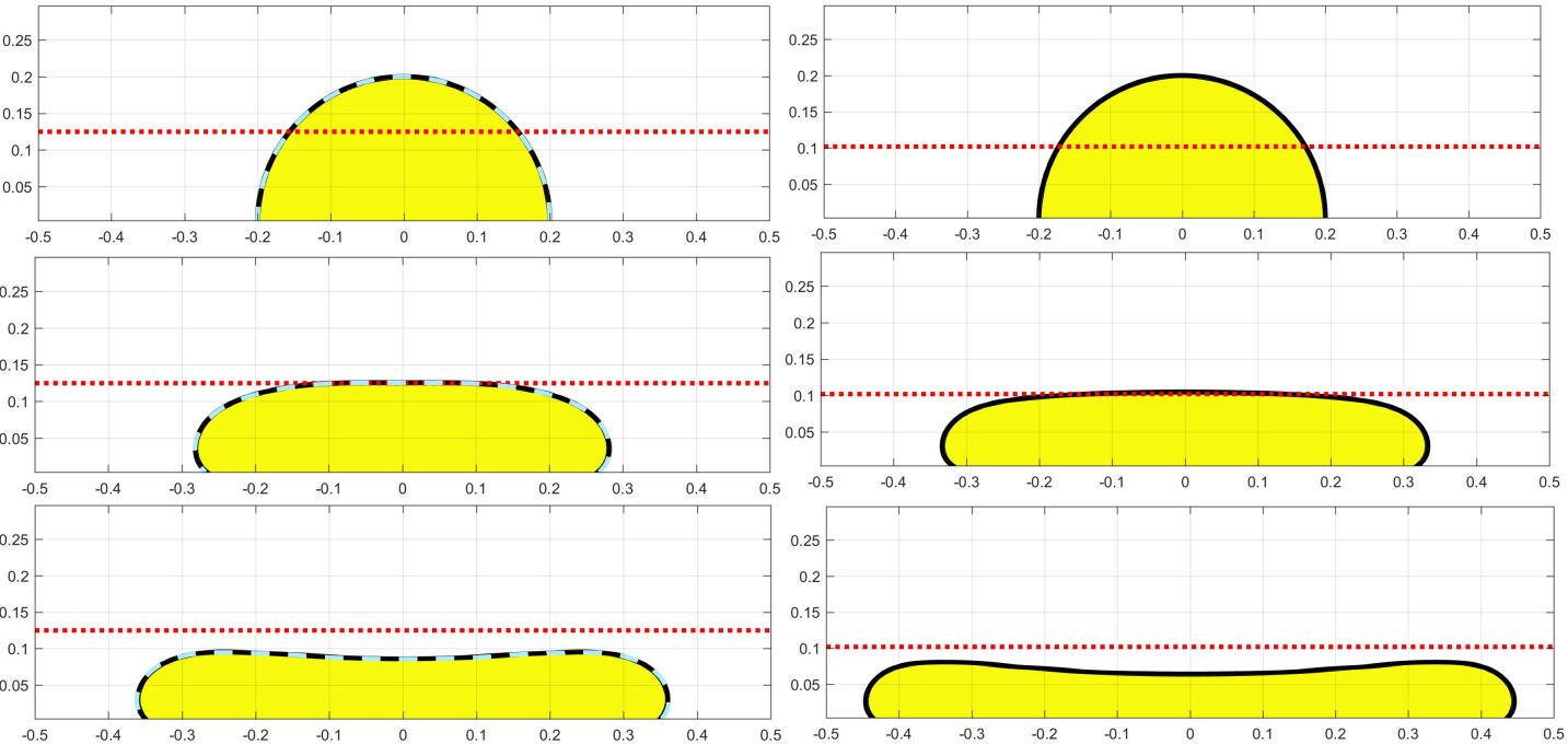
Figure 5: Evolution of the water drop using Eq.(29) with $\theta=135^{0}$. Yellow: water (Phase 1); White: air (Phase 2); Red dotted line: asymptotic solution from Eq.(38); Cyan dashed line: $N$-phase solution from Eq.(32) with $\phi_{3}|_{t=0}=-1$. Left column: $|\mathbf{g}|=10$; Right column: $|\mathbf{g}|=15$. From top to bottom, $t=0.0$, $t=0.2$, $t=0.4$, $t=1.0$, $t=1.4$, and $t=3.0$.

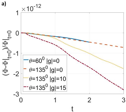
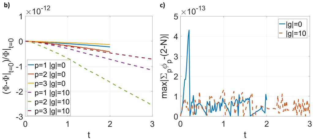
Figure 6: a) Relative changes of $\Phi$ ($=\int_{\Omega}\phi d\Omega$) from the two-phase solutions versus time. b) Relative changes of $\Phi$ from the $N$-phase solutions versus time ($p$ is the phase index). c) $\max|\sum_{p}\phi_{p}-(2-N)|$ from the $N$-phase solutions versus time.

Next, we supplement results of the $N$-phase model Eq.(32). The oil phase (Phase 3) is introduced, whose material properties are listed in Table 2 as well. The domain size becomes $[-1,1]\times[0,0.5]$ while the grid size is the same as the two-phase cases. The water drop right now is on the bottom wall with a contact angle $\theta_{1,2}=60^{0}$, while the oil drop is attached to the top wall with a contact angle $\theta_{3,2}=120^{0}$. Evolution of the drops is shown in Fig.7. Not only both the water and oil drops finally match the exact solution Eq.(37) but also the shape of the water drop at different moments is indistinguishable from the two-phase solution in the left column of Fig.2. The final heights and spreading lengths of the two drops are measured and plotted in Fig.3 a) as well, and good agreement is obtained with both the exact and two-phase solutions. Fig.4 also shows the convergence behavior of the $N$-phase model Eq.(32). The behavior is similar to the two-phase one Eq.(29) in Fig.4 a) in terms of the height and spreading length of the water drop. Convergence in between 1st and 2nd order is again observed in Fig.4 b) in terms of $t_{c}$ after which the kinetic energy ($E_{K}=\int_{\Omega}\frac{1}{2}\rho\mathbf{u}\cdot\mathbf{u}d\Omega$) is less than $10^{-5}$. The kinetic energy now includes the contribution from the oil drop.

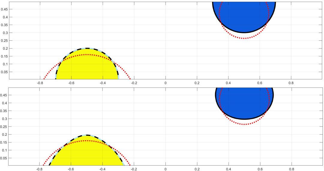
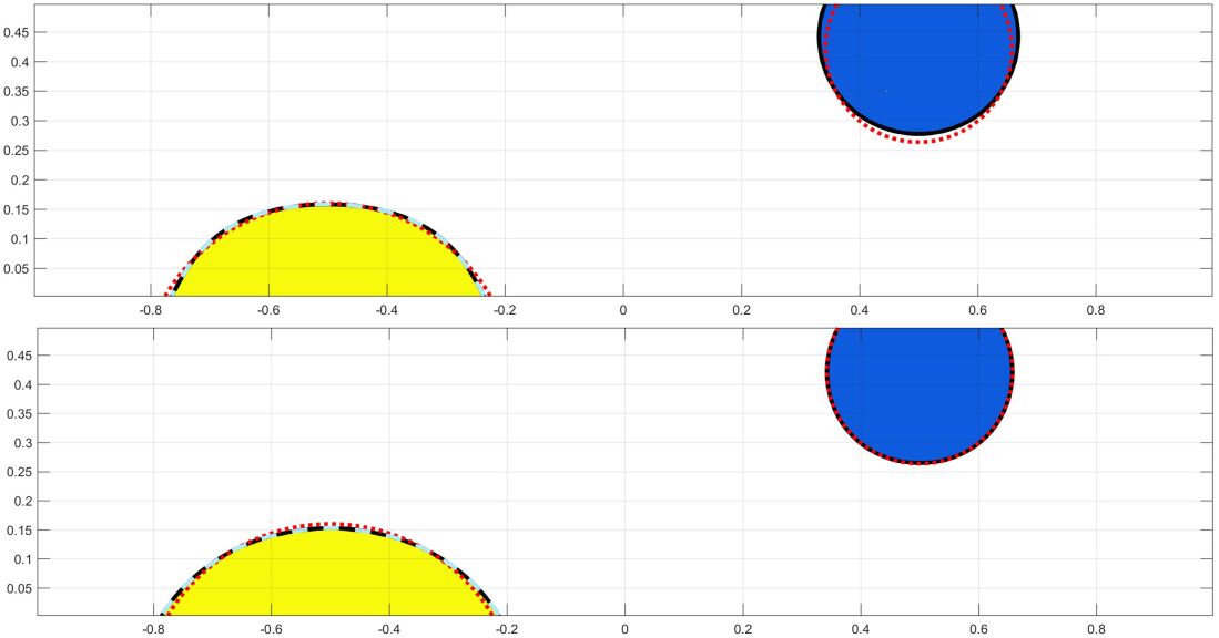
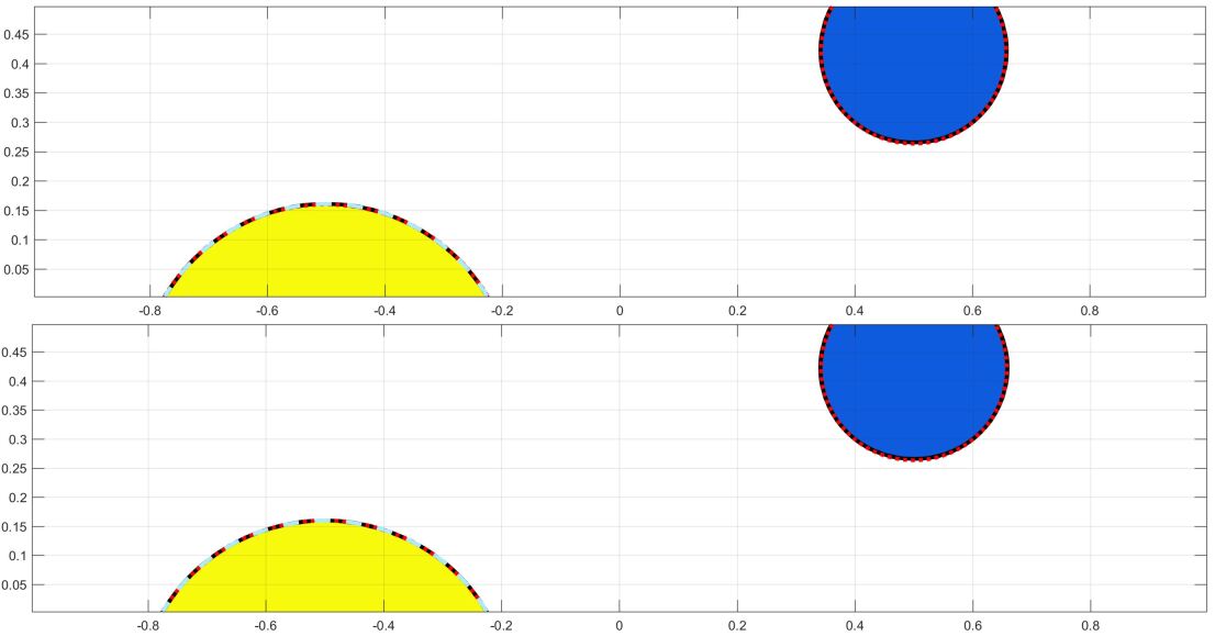
Figure 7: Evolution of the water and oil drops using Eq.(32) with $|\mathbf{g}|=0$, $\theta_{1,2}=60^{0}$, and $\theta_{3,2}=120^{0}$. Yellow: water (Phase 1); White: air (Phase 2); Blue: oil (Phase 3); Red dotted line: exact solution from Eq.(37); Cyan dashed line: two-phase solution from Eq.(29) in the left column of Fig.2. From top to bottom, $t=0.0$, $t=0.2$, $t=0.4$, $t=1.0$, $t=1.4$, and $t=2.0$.

Then, the gravity is added and the $N$-phase model Eq.(32) is again used. The surface tension between the oil and air is adjusted so that the final heights of both the water and oil drops, predicted from the asymptotic solution Eq.(38), are the same. The domain is $[-1,1]\times[0,0.3]$, and the magnitude of the gravity is $|\mathbf{g}|=10$ . The contact angle of the water drop on the bottom wall is $\theta_{1,2}=135^{0}$, while it is $\theta_{3,2}=120^{0}$ for the oil drop. Evolution of the drops are shown in Fig.8. Both of the drops are compressed vertically and finally reach a similar height to the asymptotic prediction. Again, the water drop behaves identically to the two-phase solution in the left column of Fig.5. Fig.3 b) also includes the final heights of the two drops in this case, and they are in good agreement with both the asymptotic and two-phase solutions. We also investigate the mass conservation of the $N$-phase model, and the relative changes of $\Phi_{p}$, where $p$ is the index of the phases, are in the order of the round-off error, as shown in Fig.6 b). In additional to that, the summation of the order parameters exactly satisfies Eq.(1), which is shown in Fig.6 c).

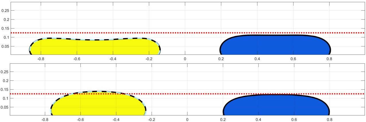
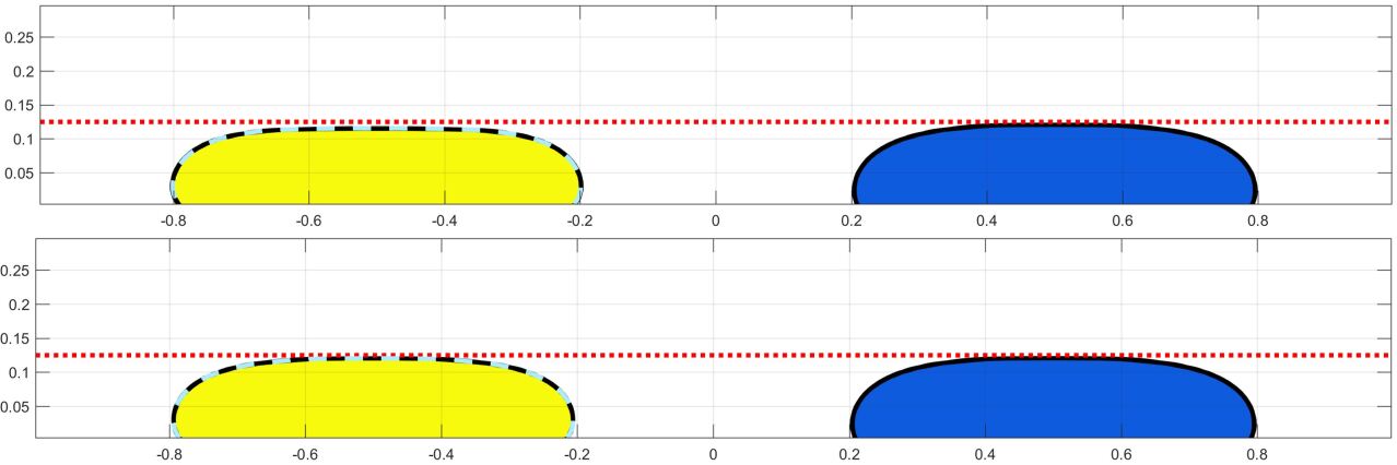
Figure 8: Evolution of the water and oil drops using Eq.(32) with $|\mathbf{g}|=10$, $\theta_{1,2}=135^{0}$, and $\theta_{3,2}=120^{0}$. Yellow: water (Phase 1); White: air (Phase 2); Blue: oil (Phase 3); Red dotted line: asymptotic solution from Eq.(37); Cyan dashed line: two-phase solution from Eq.(29) in the left column of Fig.5. From top to bottom, $t=0.0$, $t=0.2$, $t=0.4$, $t=1.0$, $t=1.4$, and $t=3.0$.

The last property the $N$-phase model should satisfy is the consistency of reduction. We repeat the $N$-phase case with $|\mathbf{g}|=10$ but only consider the left half of the domain, i.e., $-1\leqslant x\leqslant 0$. Therefore, the oil drop disappears at the beginning, i.e., $\phi_{3}|_{t=0}=-1$. Evolution of the water drop from the $N$-phase model is shown in the left column of Fig.5 as well using the cyan dashed line, and the difference from the two-phase solution is negligible. This also suggests that choosing $g_{w}(\phi)$ in Eq.(28) as a Sine or Hermite polynomial function has a negligible effect on the solution. Fig.9 quantitatively validates that not only the mass conservation and the summation of the order parameters are exactly satisfied by the $N$-phase model Eq.(32) but also the consistency of reduction since $\phi_{3}=-1$ is true at $\forall t>0$.

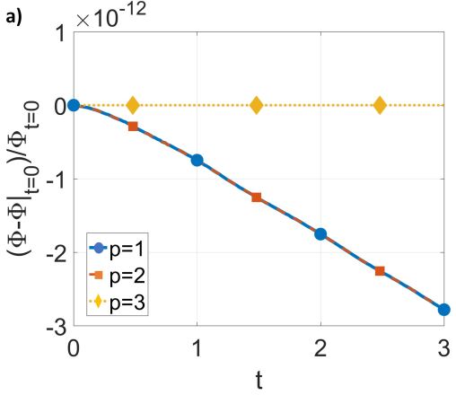
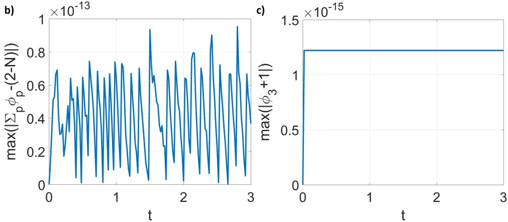
Figure 9: a) Relative changes of $\Phi$ ($=\int_{\Omega}\phi d\Omega$) from the $N$-phase solution versus time ($p$ is the phase index) with $\phi_{3}|_{t=0}=-1$. b) $\max|\sum_{p}\phi_{p}-(2-N)|$ from the $N$-phase solutions versus time with $\phi_{3}|_{t=0}=-1$. c) $\max|\phi_{3}+1|$ from the $N$-phase solutions versus time with $\phi_{3}|_{t=0}=-1$.

4.2 Couette flow

To demonstrate the proposed formulation in moving contact line problems, we consider the Couette flow in a reference frame moving with the contact line. The same problem was performed in (Yueetal2010, ) to study the contact line dynamics of the Cahn-Hilliard model. Following the setup in (Yueetal2010, ), we consider a channel having a height $L$ and a length $4L$, see the schematic in Fig.10 a).

Figure 10: Schematics of a) the Couette flow, and b) the Poiseuille flow.

The top wall of the channel is moving horizontally with a velocity $U$, while the bottom wall is moving oppositely with the same speed. The steady state solution of the problem corresponds to a contact line moving at a constant speed $U$ with respect to a fixed bottom wall. Like those in (Yueetal2010, ), the capillary number is $Ca=\frac{\mu_{1}U}{\sigma}=0.02$, the viscosity ratio is $\mu^{*}=\frac{\mu_{2}}{\mu_{1}}=1$, and the inertia is neglected. Another dimensionless number related to the mobility in the conservative Allen-Cahn model is $S_{CAC}=\mu_{1}M=0.1$. The channel is discretized by $400\times 100$ grid cells, and the time step size is $\frac{U\Delta t}{L}=1\times 10^{-4}$. The homogeneous Neumann boundary condition is used at the left and right boundaries, while the no-slip boundary condition is used at the top and bottom. The contact angle at the top wall is either $\theta=90^{0}$ or $\theta=120^{0}$, and the same at the bottom. The interface is initially vertical and the initial velocity is identical to the steady state Couette flow without interfaces, i.e., $\mathbf{u}_{C}=\left\{\frac{2U}{L}\left(y-\frac{L}{2}\right),0\right\}$.

As shown in Fig.11, the steady state results from the proposed formulation agree very will with those reported in (Yueetal2010, ) using the Cahn-Hilliard model, no matter the contact angle at the top and bottom walls is $90^{0}$ or $120^{0}$. Since only the steady state results of the problem are provided in (Yueetal2010, ), we supplement the transitional results from the consistent and conservative Phase-Field method (Huangetal2020, ) which uses the same Cahn-Hilliard model as the one in (Yueetal2010, ). The transitional results correspond to the acceleration of the moving contact line before it reaches the final speed $U$. Again in Fig.11, not only the steady state results but also the transitional ones from the proposed formulation match those from the Cahn-Hilliard model very well.

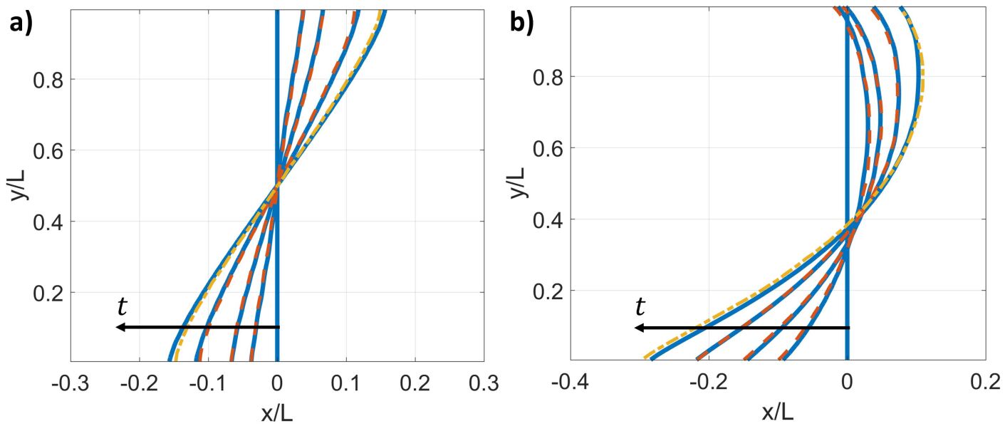
Figure 11: Results of the Couette flow. a) $\theta=90^{0}$. b) $\theta=120^{0}$. Blue solid lines: Interface at $\frac{Ut}{L}=0.00$, $0.05$, $0.10$, $0.25$, and steady state, from the proposed formulation with the conservative Allen-Cahn model. Yellow dash-dotted line: Interface at steady state from (Yueetal2010, ) using the Cahn-Hilliard model. Red dashed lines: Interface at $\frac{Ut}{L}=0.05$, $0.10$, and $0.25$, from the consistent and conservative Phase-Field method (Huangetal2020, ) using the same Cahn-Hilliard model as the one in (Yueetal2010, ).

4.3 Poiseuille flow

The Poiseuille flow in a reference frame moving with the contact line, reported in (Yueetal2010, ), is also considered, see the schematic in Fig.10 b). It corresponds to a fluid displacing another fluid in a capillary tube. The domain is an axisymmetric capillary tube with a radius $L$ and a length $6L$. The tube wall is moving backward with a velocity $U$, which is the average velocity of the fully-developed Poiseuille flow without interfaces, i.e., $\mathbf{u}_{P}=\{0,\frac{2U}{L^{2}}(L^{2}-x^{2})\}$. The dimensionless numbers $Ca$, $\mu^{*}$, and $S_{CAC}=0.1$ are defined identically to those in the Couette flow Section 4.2. The capillary tube is discretized by $100\times 600$ grid cells, and the time step size is $\frac{U\Delta t}{L}=1\times 10^{-4}$. The no-slip boundary condition is used at the tube wall, and the contact angle there is $\theta$. The Dirichlet boundary condition is used at the inlet and outlet with a velocity $\mathbf{u}_{io}=\{0,\frac{2U}{L^{2}}(L^{2}-x^{2})-U\}$. The interface is initially vertical, and the initial velocity is identical to $\mathbf{u}_{io}$.

As shown in Fig.12 a), the steady state interface from the proposed formulation agrees well with the one in (Yueetal2010, ) using the Cahn-Hilliard model, with $Ca=0.02$, $\mu^{*}=1$, and $\theta=90^{0}$. Notice that the coordinate system shown in Fig.12 a) has been adapted to the one in (Yueetal2010, ) such that $x/L=0$ is at the tube wall and $x/L=1$ at the axis of symmetry. Further, we consider the apparent contact angle $\theta_{M}$ versus the capillary number $Ca$ with $\mu^{*}=0.9$ and $\theta=98^{0}$. Like those in (Yueetal2010, ) and the references therein, the apparent contact angle is obtained from $\theta_{M}=\arccos(-L/R)$, under the assumption that the interface is a spherical cap with a radius $R$, as illustrated in Fig.10 b). In Fig.12 b), results from the proposed formulation agree with both from the Cahn-Hilliard model (Yueetal2010, ) and the celebrated theory of Cox (Cox1986, ). In (Yueetal2010, ), the adaptive mesh refinement (AMR) has been implemented. With a smaller $Ca$, the interface is less deformed. Then, AMR is able to locally increase the resolution near the interface, which is favorable in improving accuracy. This explains the minor discrepancy in Fig.12 b) when $Ca\leqslant 0.01$.

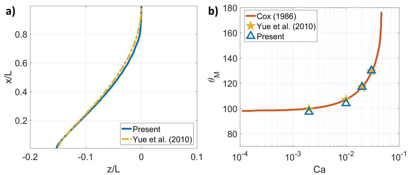
Figure 12: Results of the Poiseuille flow. a) Steady state interface with $Ca=0.02$, $\mu^{*}=1$, and $\theta=90^{0}$. The coordinate system has been adapted to the one in Yue et al. (2010) (Yueetal2010, ) such that $x/L=0$ is at the tube wall and $x/L=1$ at the axis of symmetry. b) Apparent contact angle $\theta_{M}$ versus capillary number $Ca$, with $\mu^{*}=0.9$ and $\theta=98^{0}$, from the proposed formulation with the conservative Allen-Cahn model, Yue et al. (2010) (Yueetal2010, ) using the Cahn-Hilliard model, and the theory of Cox (1986) (Cox1986, ).

In the present section and Section 4.2, the Cahn-Hillard results from (Yueetal2010, ) used the dimensionless diffusion length $S_{CH}=\sqrt{\mu_{1}M_{CH}}/L=0.01$, where $M_{CH}$ is the mobility in the Cahn-Hilliard model. Moreover, the authors of (Yueetal2010, ) related the dimensionless slip length in Cox’s formula to $2.5S_{CH}$, which is used in Fig.12 b). We discovery that quantitative matches between the Cahn-Hilliard model and the proposed formulation with the conservative Allen-Cahn model in contact-line dynamics are obtained if we correspond $S_{CH}=0.01$ of the Cahn-Hilliard model to $S_{CAC}=0.1$ of the conservative Allen-Cahn model. To further verify, explain, and generalize such a correspondence between the two Phase-Field models in contact-line dynamics will be interesting, but needs non-trivial additional works and is outside the scope of the present study.

4.4 Spreading drop

To further demonstrate the proposed formulation in dynamical problems with inertia, we consider spreading of a drop on a solid substrate, reported in (Renardyetal2001, ) using the Volume-of-Fluid (VoF) method. The setup in (Renardyetal2001, ) is followed: The computational domain is $[0,1]\times[0,1]$, whose left and right boundaries are periodic, and the top and bottom are no-slip. A circular drop of Phase 1 with a radius of $R_{0}=0.2$ is centered at $(0.5,0.85)$ and surrounded by Phase 2. The contact angle at the top wall is set to be $\theta=70.53^{0}$. The two phases have a matched density $\rho=0.1$ and viscosity $\mu=0.001$, and the surface tension between them is $\sigma=0.03$. The mobility follows $M\lambda=8\times 10^{-3}$. The domain is discretized by $128\times 128$ grid cells, and the time step size is $\Delta t=1\times 10^{-4}$. Using the inertia-capillary time scale $T=\sqrt{\frac{\rho R_{0}^{3}}{\sigma}}$ to determine the velocity scale, i.e., $U=\frac{R_{0}}{T}$, the Reynolds number and capillary number in this problem are $Re=\frac{\rho UR_{0}}{\mu}=24.5$ and $Ca=\frac{\mu U}{\sigma}=0.04$, respectively.

The dynamical process of the problem is shown in Fig.13. The initial configuration of the drop and the top wall intersect with an angle different from the assigned contact angle. Such a difference drives the drop to spread and deform, and finally reach the equilibrium shape. For comparison, the results in (Renardyetal2001, ) using the Volume-of-Fluid method are also plotted in Fig.13. The entire process predicted by the proposed formulation agrees very well with those in (Renardyetal2001, ), which demonstrates the effectiveness of the proposed formulation.

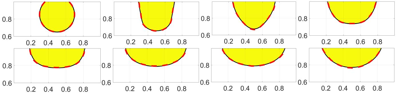
Figure 13: Results of the spreading drop. From left to right, top to bottom, $t=0.0$, $0.1$, $0.2$, $0.3$, $0.4$, $0.5$, $0.6$, and $1.0$. Results from the proposed formulation with the conservative Allen-Cahn model label Phase 1 in yellow and Phase 2 in white. Results from (Renardyetal2001, ) using the Volume-of-Fluid (VoF) method are denoted by red dashed lines.

4.5 Axisymmetric spreading drop

Here, we present spreading of an axisymmetric drop on a solid substrate, mimicking the experiment in (Eddietal2013, ). The liquid drop is a mixture of Glycerine (79%) and water (21%), and its material properties are listed in Table 3, along with those of the surrounding air. The contact angle at the substrate is $\theta=85^{0}$. Initially, the spherical drop of a radius $R_{0}=0.5\mathrm{mm}$ is released at $z=R_{0}$, in contact with the solid substrate at $z=0$.

Table 3: Material properties in the axisymmetric spreading drop

The specific computational setup is as follows. We use a length scale $L_{\mathrm{ref}}=2R_{0}=1\mathrm{mm}$, density scale $\rho_{\mathrm{ref}}=1\mathrm{kg/m^{3}}$, and acceleration scale $a_{\mathrm{ref}}=1\mathrm{m/s^{2}}$ to non-dimensionalize the governing equations. As a result, the computational domain is $[0,1]\times[0,1.25]$. The top and right boundaries are the outflow boundary, the left is the axis of symmetric, and the bottom is the no-slip wall. Like in Section 4.4, the mobility follows $M\lambda=8\times 10^{-3}$. The domain is discretized by $128\times 160$ grid cells, and the time step size is $\Delta t=5\times 10^{-5}$.

Fig.14 shows the results in their dimensional forms. The evolution of the drop is shown in Fig.14 a), along with the exact steady state solution with a zero gravity. The exact solution is obtained by matching the volume of a spherical cap to the volume of the liquid drop, i.e., $\frac{4}{3}\pi R_{0}^{3}=\frac{1}{3}\pi h^{2}(3R-h)$ where $R$ and $h=R(1-\cos(\theta))$ are the radius and height of the spherical cap, respectively. From Table 3, one can compute the Eötvös (or Bond) number $Eo=\frac{\rho_{1}|\mathbf{g}|R_{0}^{2}}{\sigma}=0.0456$, which represents the ratio of the gravity force to the surface tension. With such a small $Eo$, the drop should finally be very close to the exact solution with a zero gravity, which is the case shown in Fig.14 a). Fig.14 b) shows the radius of the wetted area versus time. The present results are compared to the experimental data in (Eddietal2013, ), and a good agreement is achieved. The major dynamics are well captured but one may notice that the present results report a smoother transition than the experimental one in the approach of the drop to the stationary state. The difference is in an acceptable range, and can be caused by the experimental uncertainties, such as the roughness of the substrate. The mobility in Sections 4.4 and 4.5 is obtained by trial and error, and the general trend we observed is that the contact line moves faster as the mobility increases. We expect future studies on theoretical analyses of the contact line dynamics of the conservative Allen-Cahn or the 2nd-order Phase-Field models, like (Jacqmin2000, ; Qianetal2006, ; Yueetal2010, ; YueFeng2011, ; Xuetal2018, ) for the Cahn-Hilliard model, will provide more insights.

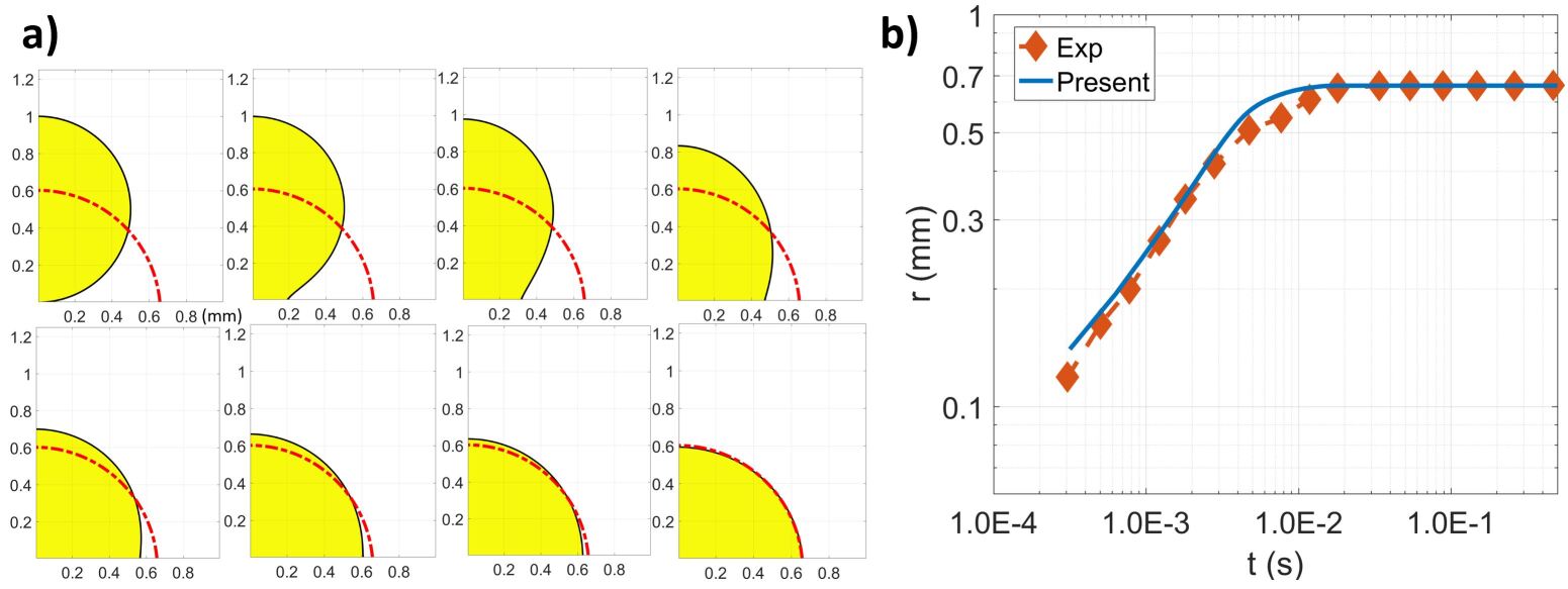
Figure 14: Results of the axisymmetric spreading drop. a) Evolution of the drop. The $x$ ($r$) axis is horizontal, the $z$ axis is vertical, and the unit is millimeter (mm). From left to right, top to bottom, $t=0\mathrm{s}$, $6.32\times 10^{-4}\mathrm{s}$, $1.58\times 10^{-3}\mathrm{s}$, $3.16\times 10^{-3}\mathrm{s}$, $4.74\times 10^{-3}\mathrm{s}$, $6.32\times 10^{-3}\mathrm{s}$, $7.91\times 10^{-3}\mathrm{s}$, and steady state. Yellow: Liquid. White: Air. Red dashdotted line: exact steady state solution with a zero gravity. b) Radius $r$ (mm) of the wetted area versus time $t$ (s). The experimental data are from (Eddietal2013, ).

So far, we have demonstrated the proposed formulation with the conservative Allen-Cahn model in various equilibrium and dynamical problems quantitatively. The remaining cases will show some potential applications and most of those results are reported qualitatively.

4.6 Bouncing drop

Here, we consider a falling water drop bouncing back after it contacts the bottom wall, using the two-phase model Eq.(29). The circular drop, surrounded by the air, has a radius $R_{0}=1.25\mathrm{mm}$, and is released above the bottom wall. The distance from the drop center to the bottom wall is $H_{0}=4R_{0}=5\mathrm{mm}$. The material properties of the fluid phases considered are listed in Table 4.

Table 4: Material properties in the bouncing drop

In the computation, non-dimensionalization is performed to the governing equations, based on $\rho_{2}$ (the air density), $H_{0}$ (the release height), and $a_{\mathrm{ref}}=1\mathrm{m/s^{2}}$ as the density, length, and acceleration scales, respectively. The acceleration scale is chosen for convenience so that the dimensionless value of the gravity is the same as the dimensional one. After the non-dimensionalization, the computational domain is $[-0.5,0.5]\times[0,1.5]$, and the circular drop is initially at $(0,1)$. The length of the domain is $4$ times the initial radius of the drop to prevent the drop from touching the lateral sides of the domain in the investigated cases of $\theta>90^{0}$. The boundaries are periodic at the lateral sides while no-slip at the top and bottom walls. The dimensionless grid size and time step are $h=0.01$ and $\Delta t=5\times 10^{-5}$, respectively. All the results reported in this section are in their dimensionless forms.

Fig.15 shows results with contact angle $\theta=165^{0}$ at the bottom wall. The drop remains circular as it is falling down. After the drop impacts on the bottom wall, it is strongly deformed to reduce the downward velocity and finally reaches a “dumbbells-like” shape. Then, the drop tries to restore the circular shape and jumps upward, leaving the bottom wall and finally arriving at a height lower than where it is initially released. This process repeats and the velocity is gradually reduced to zero. Finally, the drop settles down on the bottom wall and the equilibrium shape deviates slightly from the circular one because of the gravity.

Different contact angles at the bottom wall are considered. We observe that the drop is unable to bounce back when the contact angle is less than or equal to $120^{0}$ and the water finally fills the bottom of the domain when the contact angle is less than or equal to $90^{0}$. The same behaviors are also reported in (Dong2012, ). Fig.17 shows shapes of the drops from different contact angles at $t=0.46$, right after the first impact to the bottom wall, and at $t=4.00$. The ($y$-component) center of mass of the drop $y_{c}$ ($y_{c}=\int_{\Omega}y\frac{1+\phi}{2}d\Omega/\int_{\Omega}\frac{1+\phi}{2}d\Omega$) versus time is shown in Fig.18 a). Until the second impact to the bottom wall, the centers of mass from $\theta=165^{0}$ and $\theta=150^{0}$ move very similarly, as shown in Fig.18 a). However, with a smaller contact angle, length of the drop in contact with the bottom wall is larger, as shown in Fig.17. This can provide more dissipation, and as a result, the drop have a less chance to bounce back. On the other hand, each time when the drop impacts to the wall induces a large deformation of the drop, which also produces a strong dissipation due to the viscosity of the water. Therefore, from Fig.18 a), peaks of the curves describing the motion of center of mass decay very fast for the drops that bounce back, e.g., those with $\theta=165^{0}$ and $150^{0}$. For the drop that is unable to bounce back, e.g., the one with $\theta=120^{0}$, it oscillates on the bottom wall, and its center of mass curve has a higher frequency but there is less attenuation between the two neighboring peaks. For the drop that will finally fill the bottom, e.g., those with $\theta=90^{0}$ and $\theta=60^{0}$, we observe a long-term but small-amplitude oscillation of the center of mass. This is caused by the capillary wave on the horizontal water-air interface, as shown in Fig.17.

Finally, we consider the effect of the mobility $M$. Fig.19 shows shapes of the drops with different mobilities (or $M\lambda$), and the mass centers ($y$ component) are shown in Fig.18 b). With a larger mobility, the drop becomes more “rigid” and therefore less deforms, as shown in Fig.19. On the other hand, a too “soft” drop, resulting from a small mobility, suffers from fictitious oscillation on the side close to the bottom wall. Even worse, the oscillation destroys the symmetry of the solution, and at the end produces a non-symmetry drop staying biased to left half of the domain. The drop with the smallest mobility finally is floating above the bottom wall because the interface is over-thickened. However, these unphysical behaviors are not observed in the cases with a larger mobility. As shown in Fig.18 b), there is no significant difference due to the mobility before the first impact of the drop to the bottom wall. The one with the largest mobility can only bounce back once and settles down very fast. The one with the smallest mobility bounces back multiple times although the height it returns to after the first impact is lowest among the three cases. These behaviors suggest that a larger mobility produces more dissipation.

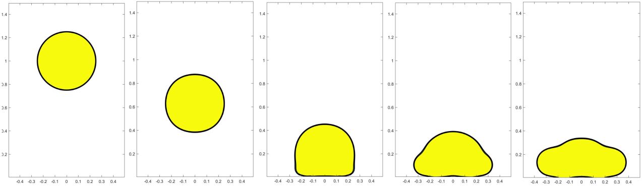
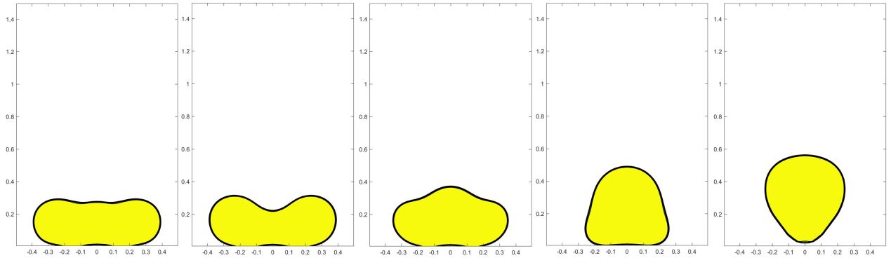
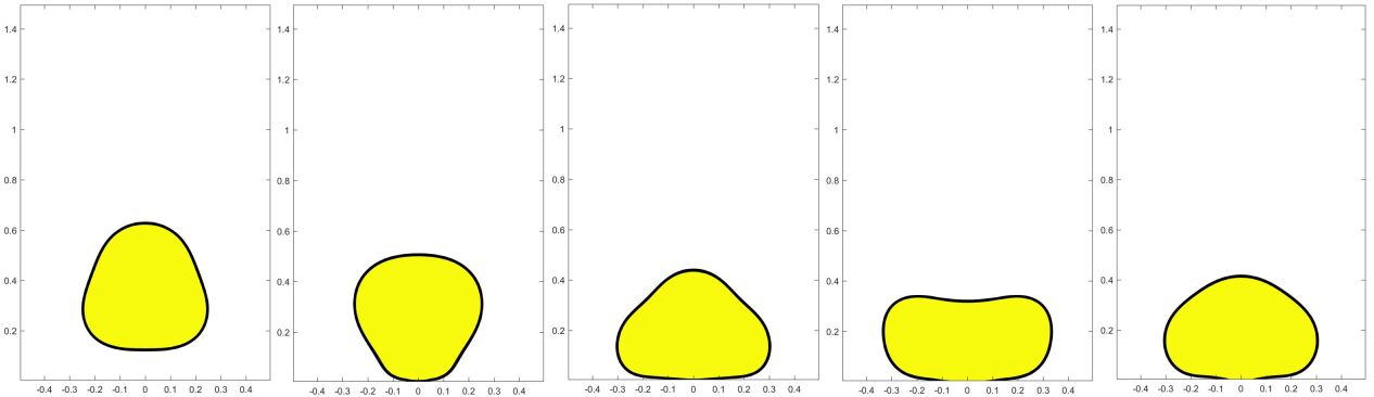
Figure 15: Results of the bouncing drop using the two-phase model Eq.(29) with $\theta=165^{0}$. Yellow: water (Phase 1); White: air (Phase 2); From left to right and top to bottom: $t=0.00$, $t=0.30$, $t=0.44$, $t=0.46$, $t=0.48$, $t=0.50$, $t=0.52$, $t=0.56$, $t=0.60$, $t=0.64$, $t=0.68$, $t=0.72$, $t=0.80$, $t=0.85$, $t=0.90$, $t=1.00$, $t=1.05$, $t=1.10$, $t=1.15$, and $t=1.20$.

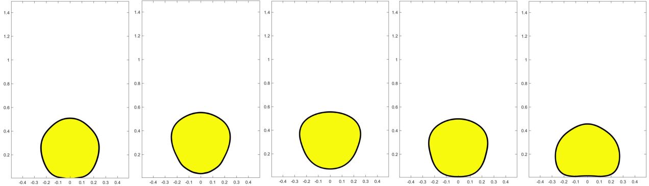
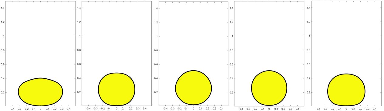
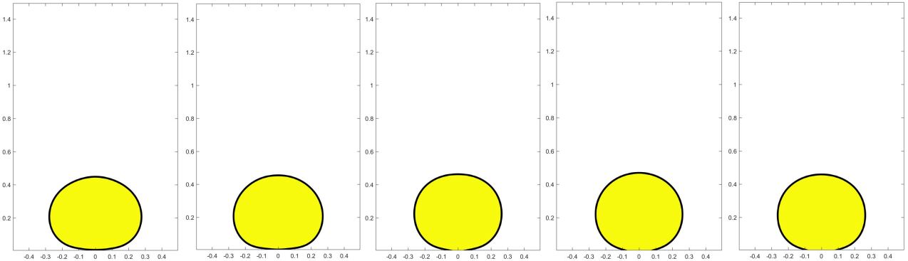
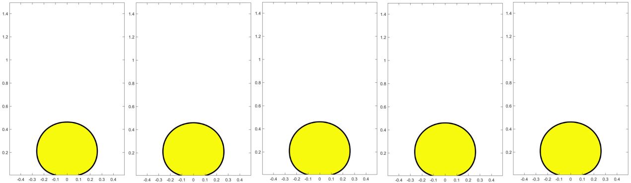
Figure 16: From left to right and top to bottom: $t=1.25$, $t=1.30$, $t=1.40$, $t=1.50$, $t=1.55$, $t=1.60$, $t=1.70$, $t=1.75$, $t=1.80$, $t=1.90$, $t=1.95$, $t=2.00$, $t=2.05$, $t=2.15$, $t=2.20$, $t=2.35$, $t=2.50$, $t=3.00$, $t=3.50$, and $t=4.00$.

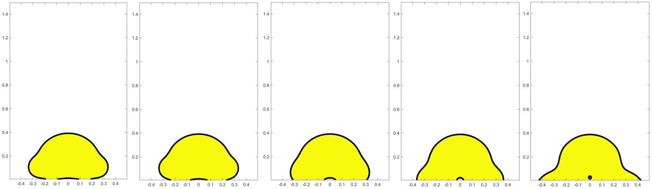
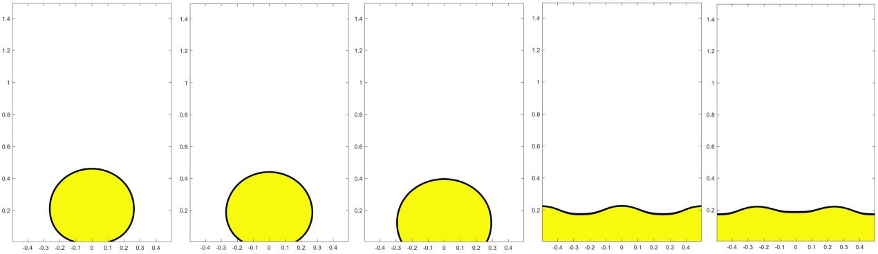
Figure 17: Shapes of the drops with different contact angles. Yellow: water (Phase 1); White: air (Phase 2); From left to right: $\theta=165^{0}$, $\theta=150^{0}$, $\theta=120^{0}$, $\theta=90^{0}$, and $\theta=60^{0}$. Top: $t=0.46$; Bottom: $t=4.00$.

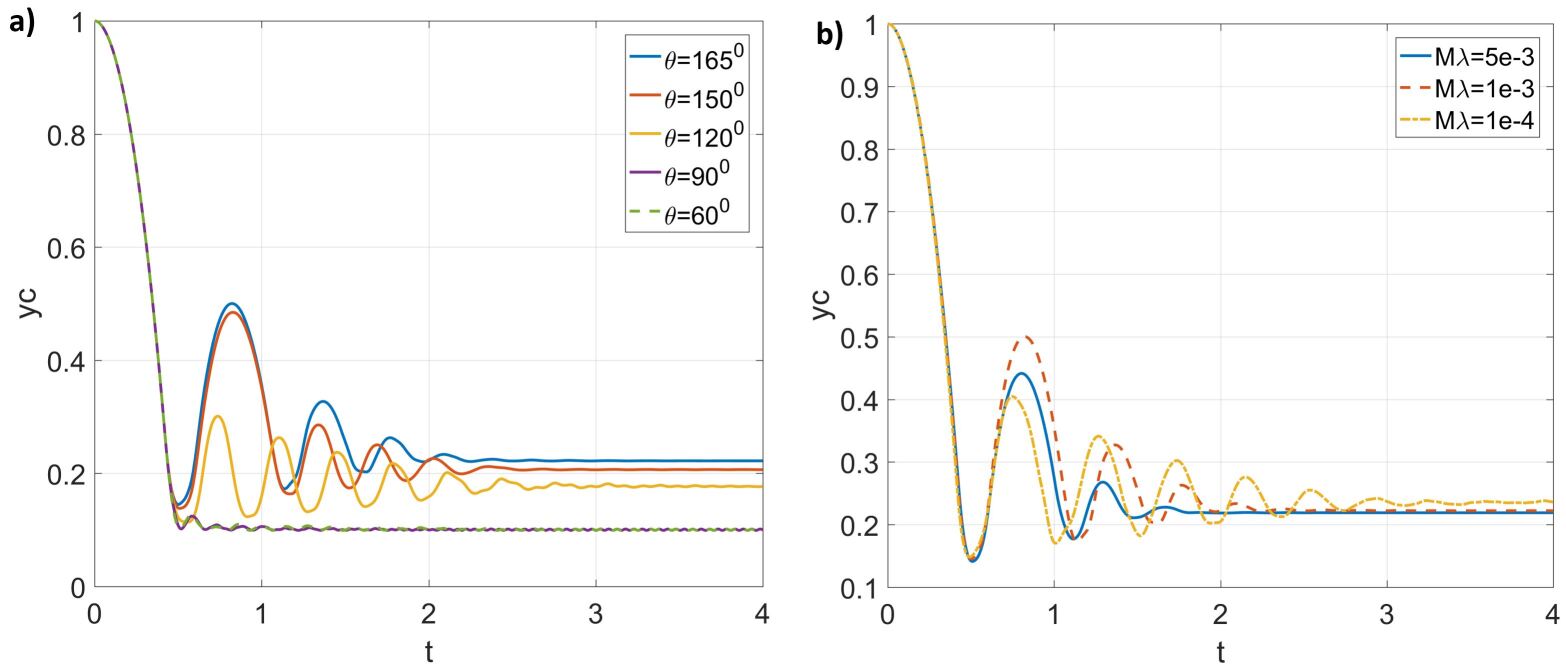
Figure 18: Mass center ($y$ component) of the drop versus time a) with different contact angles, b) with different mobilities.

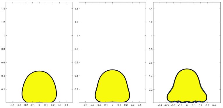
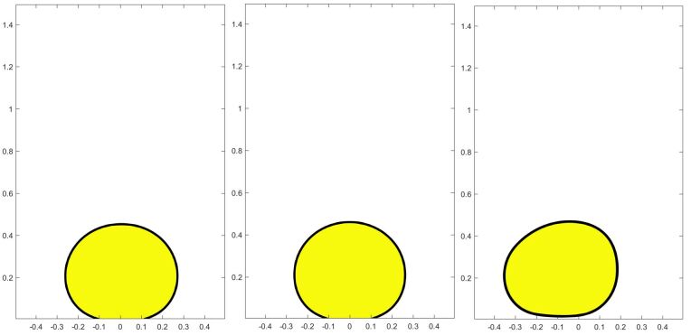
Figure 19: Shapes of the drops with different mobilities. Yellow: water (Phase 1); White: air (Phase 2); From left to right: $M\lambda=5\times 10^{-3}$, $M\lambda=1\times 10^{-3}$, and $M\lambda=1\times 10^{-4}$. Top: $t=0.60$; Bottom: $t=4.00$.

4.7 Compound drop

Here, we report a compound drop sliding on a horizontal solid wall using the $N$-phase model Eq.(32). Initially, the compound drop is semicircular with a radius $R_{0}$, composed of two quarter-circular drops. The left and right quarters are full of Phases 1 and 2, respectively, and they are surrounded by Phase 3. The Reynolds number and capillary number considered are $Re=\rho_{1}UR_{0}/\mu_{1}=10$ and $Ca=\mu_{1}U/\sigma_{1,2}=0.1$, respectively. Here, $U$ is determined from the inertia-capillary time scale $T=\sqrt{\rho_{1}R_{0}^{3}/\sigma_{1,2}}$, i.e., $U=R_{0}/T$, which leads to the Weber number $We=\rho_{1}U^{2}R_{0}/\sigma_{1,2}=1$. The material properties of the other two phases are related to $\rho_{1}$, $\mu_{1}$, and $\sigma_{1,2}$, and are listed in Table 5.

Table 5: Material properties in the compound drop

The computational domain is $[-2R_{0},2R_{0}]\times[0R_{0},1.2R_{0}]$, and the periodic and no-slip boundary conditions are assigned along the $x$ and $y$ axes, respectively. The compound drop is initially on the middle of the bottom wall. The space and time are discretized by $200\times 60$ grid cells and $U\Delta t/R_{0}=1\times 10^{-4}$. Evolution of the drops are shown in Fig.20, along with the exact solution from (Zhangetal2016, ) for the equilibrium state. The drops move towards the equilibrium shape, which agrees well with the exact solution. Quantitatively, the spreading lengths (normalized by $R_{0}$) of Phases 1 and 2 are $1.0547$ and $1.6871$, respectively, and the relative errors are 1.614% and 1.166% after comparing to the exact ones $1.0720$ and $1.7070$ from (Zhangetal2016, ).

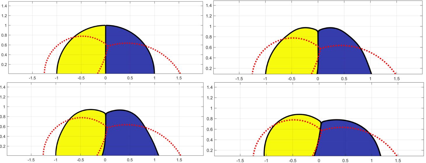
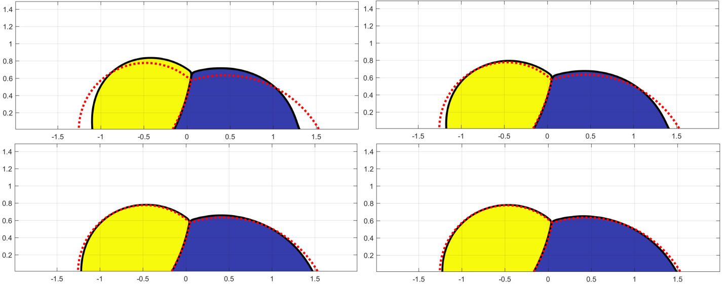
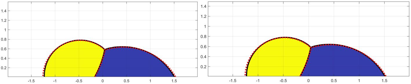
Figure 20: Evolution of the compound drop using Eq.(32) with a stationary bottom wall. The coordinate has been normalized by the initial radius of the compound drop $R_{0}$. Yellow: Phase 1; Blue: Phase 2; White: Phase 3; Red dotted line: exact solution from (Zhangetal2016, ). From top to bottom and left to right: $Ut/R_{0}=0.0$, $0.2$, $0.4$, $1.0$, $1.4$, $2.0$, $3.0$, $4.0$, $5.0$ and $6.0$, where $U=\sqrt{\sigma_{1,2}/(\rho_{1}R_{0})}$ is the inertia-capillary velocity scale.

Next, we investigate sliding motion of the compound drop when the bottom wall is moving backward with a speed $U$, and the setup is slightly changed as follows. Using the speed of the bottom wall, the corresponding Reynolds number, capillary number, and Weber number considered are $Re=\rho_{1}UR_{0}/\mu_{1}=66.6$, $Ca=\mu_{1}U/\sigma_{1,2}=0.075$, and $We=\rho_{1}U^{2}R_{0}/\sigma_{1,2}=5$, respectively. The dynamic viscosity ratios are changed to be $\mu_{2}/\mu_{1}=0.67$ and $\mu_{3}/\mu_{1}=0.33$. The domain height becomes $1.5R_{0}$, while the grid size remains the same. Results are shown in Fig.21, and the behaviors of the drops are significantly different from those on a stationary wall. We observe that the Phase 1 (yellow) drop climbs onto the Phase 2 (blue) drop, and thoroughly leave the bottom wall, sitting on the Phase 2 drop. Then, it crosses the Phase 2 drop and returns on the bottom wall. At the end, the Phase 1 drop is still in contact with the Phase 2 drop but moves in front of it.

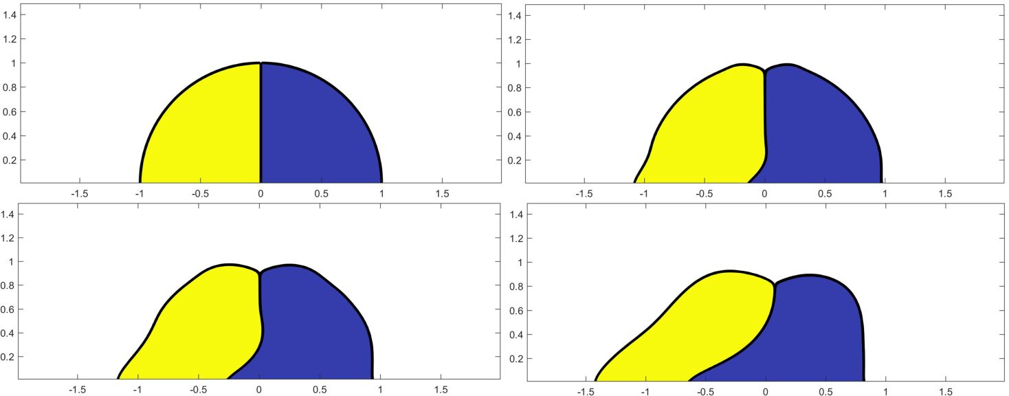
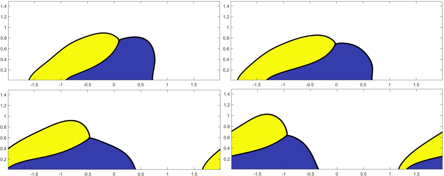
Figure 21: Evolution of the compound drop using Eq.(32) with a translating bottom wall. The coordinate has been normalized by the initial radius of the compound drop $R_{0}$. Yellow: Phase 1; Blue: Phase 2; White: Phase 3. From top to bottom and left to right: $Ut/R_{0}=0.0$, $0.2$, $0.4$, $1.0$, $1.4$, $2.0$, $3.0$, $4.0$, $5.0$, $6.0$, $7.0$, and $8.0$, where $U$ is the speed of the bottom wall.

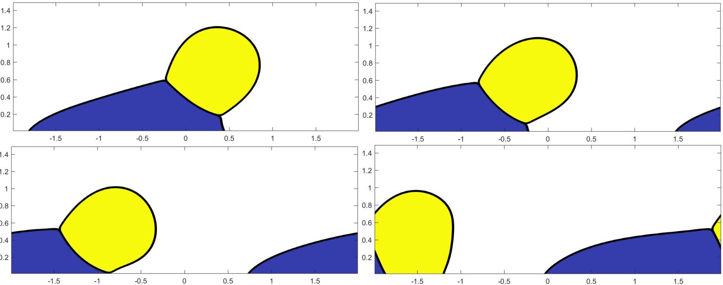
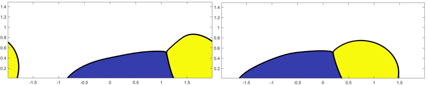
Figure 22: From top to bottom and left to right: $Ut/R_{0}=9.0$, $10.0$, $11.0$, $12.0$, $13.0$, and $14.0$, where $U$ is the speed of the bottom wall.

5 Conclusions and future works

In the present work, we proposed a general formulation to implement the contact angle boundary conditions for the second-order Phase-Field models. The original second-order Phase-Field models are modified by adding a Lagrange multiplier that enforces the mass conservation but does not change the summation of the order parameters and the consistency of reduction. The newly introduced Lagrange multiplier is determined by the consistent and conservative volume distribution algorithm (Huangetal2020B, ). The proposed formulation is applicable to not only two-phase but also $N$-phase ($N\geqslant 2$) cases. Then, this novel formulation is physically coupled to the hydrodynamics using the consistent formulation (Huangetal2020CAC, ) and can be applied to large-density-ratio problems. To demonstrate its effectiveness of moving contact line simulations, we apply the proposed formulation to the reduction-consistent multiphase conservative Allen-Cahn model (Huangetal2020B, ), whose two-phase version is equivalent to the one in (BrasselBretin2011, ). The complete system is numerically solved by the consistent and conservative scheme (Huangetal2020CAC, ; Huangetal2020B, ), which preserves the mass conservation, the summation of the order parameters, and the consistency of reduction exactly on the discrete level, as validated in the present study. Various numerical tests are performed in both 2D Cartesian and axisymmetric coordinates. The proposed formulation accurately reproduces the exact and/or asymptotic solutions for equilibrium problems, and captures important dynamical behaviors reported, e.g., in (Yueetal2010, ; Zhangetal2016, ; Dong2012, ; Dong2017, ) using the Cahn-Hilliard models which are a 4th-order Phase-Field model, in (Renardyetal2001, ) using the Volume-of-Fluid (VoF) method, and in (Eddietal2013, ) performing experiments. Since the parallelization has not been implemented, only two-dimensional and axisymmetric results are reported. The extension of the proposed formulation to three-dimensional problems is straightforward without any modifications, and the physical properties demonstrated in the present study, such as the summation of the order parameters, mass conservation, and consistency of reduction, will remain intact. However, an efficient parallel strategy with adaptive mesh refinement (AMR) is desired for three-dimensional problems, and this is a valuable future direction to proceed with the present study.

The present study leaves open the possibility of using the 2nd-order Phase-Field models for moving contact line problems, which has never been considered before. Therefore, it provides plenty of new opportunities to study in the future. Generally speaking, the accuracy of the prediction heavily relies on the properties of the Phase-Field model and the contact angle boundary condition, i.e., the definitions of $\mathcal{L}$ in Eq.(4) and $\mathcal{F}^{w}$ in Eq.(7), and on the parameters therein. Since the pool of plausible Phase-Field models for moving contact line problems is greatly expanded, it is now not only possible but also desirable to investigate and clarify their performance. Unlike the Cahn-Hilliard models, there is little theoretical analysis of the 2nd-order Phase-Field models in moving contact line problems, e.g., the asymptotic analysis as the interface thickness tends to zero. Such an analysis is important to provide physical insights of determining the parameters in the models. We expect the present study will motivate consideration of using 2nd-order Phase-Field models in moving contact line problems as the effectiveness has been demonstrated.

Appendix A Manufactured solution

Here, we perform a manufactured solution test to the two-phase conservative Allen-Cahn model including the contact angle boundary condition to further demonstrate the convergence. In this problem, we assume that the exact solutions of the order parameter, velocity, and pressure are $\phi^{E}=\cos(x)\cos(y)\sin(t)$, $u^{E}=\sin(x)\cos(y)\cos(t)$, $v^{E}=-\cos(x)\sin(y)\cos(t)$, and $P^{E}=\cos(x)\cos(y)\sin(t)$, respectively. Then, a source term $S^{BC}$ is added to the contact angle boundary condition, i.e., $\mathbf{n}\cdot\nabla\phi=\mathcal{F}^{w}[\phi;\theta]+S^{BC}$, where $S^{BC}$ is directly obtained with $\phi^{E}$, i.e., $S^{BC}=\mathbf{n}\cdot\nabla\phi^{E}-\mathcal{F}^{w}[\phi^{E};\theta]$. In a similar manner, one can obtain the source terms added to the right-hand side of the Phase-Field model Eq.(16) and the momentum equation Eq.(24). We additionally assume $Q^{E}=\cos(x)\cos(y)\sin(t)$ to obtain the source term added to the right-hand side of the consistent formulation Eq.(19). The parameters used are $\rho_{1}=3$, $\rho_{2}=1$, $\mu_{1}=0.02$, $\mu_{2}=0.01$, $\sigma=0.0094$, $\mathbf{g}=\{1,-2\}$, $\eta=0.1$, and $M=0.001$. The domain considered is $[-\pi,\pi]\times[-\pi,\pi]$ with the free-slip boundary condition. The contact angles at the boundaries are $90^{0}$ except the bottom one that is $75^{0}$. The initial conditions are $\phi^{E}$, $u^{E}$, $v^{E}$, and $P^{E}$ evaluated at $t=0$. The time step size is $\Delta t=1\times 10^{-3}$, and the computations last till $t=1$. We output $\phi$, $u$, $v$, and $P$, and depict the $L_{1}$ norms of $\phi-\phi^{E}$, $u-u^{E}$, $v-v^{E}$, and $P-P^{E}$, i.e., the averages of $|\phi-\phi^{E}|$ etc. over the domain, in Fig.23. All the variables are converging as the cell size is refined.

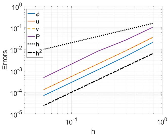
Figure 23: $L_{1}$ errors of $\phi$, $u$, $v$, and $P$ versus the cell size in the manufactured solution problem.

References

- [1] H. Abels, H. Garcke, and G. Grun. Thermodynamically consistent, frame indifferent diffuse interface models for incompressible two-phase flows with different densities. Mathematical Models and Methods in Applied Sciences, 22:1150013, 2012.
- [2] S. Afkhami, S. Zaleski, and M. Bussmann. A mesh-dependent model for applying dynamic contact angles to vof simulations. Journal of computational physics, 228(15):5370–5389, 2009.
- [3] S. Aihara, T. Takaki, and N. Takada. Multi-phase-field modeling using a conservative allen–cahn equation for multiphase flow. Computers & Fluids, 178:141–151, 2019.
- [4] S.M. Allen and J.W. Cahn. A microscopic theory for antiphase boundary motion and its application to antiphase domain coarsening. Acta Metallurgica, 27:1085–1095, 1979.
- [5] D.M. Anderson, G.B. McFadden, and A.A. Wheeler. Diffuse-interface methods in fluid mechanics. Annu. Rev. Fluid Mech., 30:139–165, 1998.
- [6] F. Bai, X. He, X. Yang, R. Zhou, and C. Wang. Three dimensional phase-field investigation of droplet formation in microfluidic flow focusing devices with experimental validation. Int. J. Multiph. Flow, 93:130–141, 2017.
- [7] F. Boyer and S. Minjeaud. Hierarchy of consistent n-component cahn–hilliard systems. Math. Models Methods Appl. Sci., 24:2885–292, 2014.
- [8] J.U. Brackbill, D.B. Kothe, and C. Zemach. A continuum method for modeling surface tension. J. Comput. Phys., 100:335–354, 1992.
- [9] M. Brassel and E. Bretin. A modified phase field approximation for mean curvature flow with conservation of the volume. Math. Methods Appl. Sci., 34:1157–1180, 2011.
- [10] J.W. Cahn and J.E. Hilliard. Free energy of a nonuniform system, i interfacial free energy. J. Chem. Phys., 28:258–267, 1958.
- [11] Z. Chai, D. Sun, H. Wang, and B. Shi. A comparative study of local and nonlocal allen-cahn equations with mass conservation. J. Fluid Mech., 122:631–642, 2018.
- [12] P-H Chiu and Y-T Lin. A conservative phase-field method for solving incompressible two-phase flows. J. Comput. Phys., 230:185–204, 2011.
- [13] R.G. Cox. The dynamics of the spreading of liquids on a solid surface. part 1. viscous flow. J. Fluid Mech., 168:169–194, 1986.
- [14] P.-G. de Gennes, F. Brochard-Wyart, and D. Quere. Capillarity and Wetting Phenomena. Springer, 2003.
- [15] H. Ding and P.D.M. Spelt. Wetting condition in diffuse interface simulations of contact line motion. Phys. Rev. E, 75:046708, 2007.
- [16] S. Dong. On imposing dynamic contact-angle boundary conditions for wall-bounded liquid-gas flows. Comput. Methods Appl. Mech. Engrg., 247-248:179–200, 2012.
- [17] S. Dong. Wall-bounded multiphase flows of n immiscible incompressible fluids: Consistency and contact-angle boundary condition. J. Comput. Phys., 338:21–67, 2017.
- [18] S. Dong. Multiphase flows of n immiscible incompressible fluids: A reduction-consistent and thermodynamically-consistent formulation and associated algorithm. J. Comput. Phys., 361:1–49, 2018.
- [19] S. Dong and J. Shen. A time-stepping scheme involving constant coefficient matrices for phase-field simulations of two-phase incompressible flows with large density ratios. J. Comput. Phys., 231:5788–5804, 2012.
- [20] A. Eddi, K.G. Winkels, and J.H. Snoeijer. Short time dynamics of viscous drop spreading. Phys. Fluids, 25:013102, 2013.
- [21] J.H. Ferziger and M. Peric. Computational Methods for Fluid Dynamics. Springer Berlin / Heidelberg, third, rev. edition. edition, 2001.
- [22] C.W. Hirt and B.D. Nichols. Volume of fluid (vof) method for the dynamics of free boundaries. J. Comput. Phys., 39:201–225, 1981.
- [23] A.A. Howard and A.M. Tartakovsky. A conservative level set method for n-phase flows with a free-energy-based surface tension model. Journal of Computational Physics, page 109955, 2020.
- [24] Y. Hu, D. Li, and Q. He. Generalized conservative phase field model and its lattice boltzmann scheme for multicomponent multiphase flows. International Journal of Multiphase Flow, 132:103432, 2020.
- [25] Z. Huang, G. Lin, and A.M. Ardekani. Consistent and conservative scheme for incompressible two-phase flows using the conservative allen-cahn model. J. Comput. Phys., 420:109718, 2020.
- [26] Z. Huang, G. Lin, and A.M. Ardekani. Consistent, essentially conservative and balanced-force phase-field method to model incompressible two-phase flows. J. Comput. Phys., 406:109192, 2020.
- [27] Z. Huang, G. Lin, and A.M. Ardekani. A consistent and conservative model and its scheme for n-phase-m-component incompressible flows. J. Comput. Phys., 434:110229, 2021.
- [28] Z. Huang, G. Lin, and A.M. Ardekani. A consistent and conservative volume distribution algorithm and its applications to multiphase flows using phase-field models. Int. J. Multiph. Flow, 142:103727, 2021.
- [29] Z. Huang, G. Lin, and A.M. Ardekani. A consistent and conservative phase-field method for multiphase incompressible flows. Journal of Computational and Applied Mathematics, 408:114116, 2022.
- [30] Z. Huang, G. Lin, and A.M. Ardekani. A consistent and conservative phase-field model for thermo-gas-liquid-solid flows including liquid-solid phase change. J. Comput. Phys., 449:110795, 2022.
- [31] D. Jacqmin. Calculation of two-phase navier-stokes flows using phase-field modeling. J. Comput. Phys., 155:96–127, 1999.
- [32] D. Jacqmin. Contact-line dynamics of a diffuse fluid interface. J. Fluid Mech., 402:57–88, 2000.
- [33] D. Jeong and J. Kim. Conservative allen–cahn–navier–stokes system for incompressible two-phase fluid flows. Comput. Fluids, 156:239–246, 2017.
- [34] G-S Jiang and C-W Shu. Efficient implementation of weighted eno schemes. J. Comput. Phys., 126:202–228, 1996.
- [35] V. Joshi and R.K. Jaiman. An adaptive variational procedure for the conservative and positivity preserving allen–cahn phase-field model. J. Comput. Phys., 336:478–504, 2018.
- [36] V. Joshi and R.K. Jaiman. A positivity preserving and conservative variational scheme for phase-field modeling of two-phase flows. J. Comput. Phys., 360:137–166, 2018.
- [37] J. Kim and H.G. Lee. A new conservative vector-valued allen-cahn equation and its fast numerical method. Comput. Phys. Commun., 221:102–108, 2017.
- [38] J. Kim, S. Lee, and Y. Choi. A conservative allen–cahn equation with a space–time dependent lagrange multiplier. Int. J. Eng. Sci., 84:11–17, 2014.
- [39] U. Lācis, P. Johansson, T. Fullana, B. Hess, G. Amberg, S. Bagheri, and S. Zaleski. Steady moving contact line of water over a no-slip substrate. The European Physical Journal Special Topics, 229(10):1897–1921, 2020.
- [40] D. Lee and J. Kim. Comparison study of the conservative allen–cahn and the cahn–hilliard equations. Math. Comput. Simulation, 119:35–56, 2016.
- [41] H.G. Lee and J. Kim. Accurate contact angle boundary conditions for the cahn–hilliard equations. Comput. Fluids, 44:178–186, 2011.
- [42] J.-C. Loudet, M. Qiu, J. Hemauer, and J.J. Feng. Drag force on a particle straddling a fluid interface: Influence of interfacial deformations. The European Physical Journal E, 43(2):1–13, 2020.
- [43] S. Manservisi and R. Scardovelli. A variational approach to the contact angle dynamics of spreading droplets. Computers & fluids, 38(2):406–424, 2009.
- [44] S. Mirjalili, C.B. Ivey, and A. Mani. A conservative diffuse interface method for two-phase flows with provable boundedness properties. J. Comput. Phys., 401:109006, 2020.
- [45] S. Mirjalili and A. Mani. Consistent, energy-conserving momentum transport for simulations of two-phase flows using the phase field equations. Journal of Computational Physics, 426:109918, 2021.
- [46] M. Muradoglu and S. Tasoglu. A front-tracking method for computational modeling of impact and spreading of viscous droplets on solid walls. Computers & Fluids, 39(4):615–625, 2010.
- [47] E. Olsson and G. Kreiss. A conservative level set method for two phase flow. J. Comput. Phys., 210:225–246, 2005.
- [48] E. Olsson, G. Kreiss, and S. Zahedi. A conservative level set method for two phase flow ii. J. Comput. Phys., 225:785–807, 2007.
- [49] S. Osher and A.J. Sethian. Fronts propagating with curvature-dependent speed: Algorithms based on hamilton-jacobi formulations. J. Comput. Phys., 79:12–49, 1988.
- [50] T. Qian, X.P. Wang, and P. Sheng. A variational approach to moving contact line hydrodynamics. J. Fluid Mech., 564:333–360, 2006.
- [51] M. Renardy, Y. Renardy, and J. Li. Numerical simulation of moving contact line problems using a volume-of-fluid method. Journal of Computational Physics, 171(1):243–263, 2001.
- [52] Y. Sato and B. Niceno. A new contact line treatment for a conservative level set method. Journal of computational physics (Print), 231(10):3887–3895, 2012.
- [53] R. Scardovelli and S. Zaleski. Direct numerical simulation of free-surface and interfacial flow. Annu. Rev. Fluid Mech., 31:567–603, 1999.
- [54] P. Seppecher. Moving contact lines in the cahn-hilliard theory. International journal of engineering science, 34(9):977–992, 1996.
- [55] J.A. Sethian and P. Smereka. Level set method for fluid interfaces. Annu. Rev. Fluid Mech., 35:341–372, 2003.
- [56] J Shen. Modeling and numerical approximation of two-phase incompressible flows by a phase-field approach. Multiscale Modeling and Analysis for Materials Simulation, 22:147–195, 2011.
- [57] J. Shen, X. Yang, and H. Yu. Efficient energy stable numerical schemes for a phase field moving contact line model. J. Comput. Phys., 284:617–630, 2015.
- [58] L. Shen, H. Huang, P. Lin, Z. Song, and S. Xu. An energy stable c0 finite element scheme for a quasi-incompressible phase-field model of moving contact line with variable density. Journal of Computational Physics, 405:109179, 2020.
- [59] Y. Shi and X.-P. Wang. Modeling and simulation of dynamics of three-component flows on solid surface. Japan Journal of Industrial and Applied Mathematics, 31(3):611–631, 2014.
- [60] P.D.M. Spelt. A level-set approach for simulations of flows with multiple moving contact lines with hysteresis. Journal of Computational physics, 207(2):389–404, 2005.
- [61] Y. Sui, H. Ding, and P.D.M. Spelt. Numerical simulations of flows with moving contact lines. Annual Review of Fluid Mechanics, 46:97–119, 2014.
- [62] J. Towns, T. Cockerill, M. Dahan, I. Foster, K. Gaither, A. Grimshaw, V. Hazlewood, S. Lathrop, D. Lifka, G.D. Peterson, R. Roskies, J.R. Scott, and N. Wilkins-Diehr. Xsede: accelerating scientific discovery. Comput. Sci. Eng., 16:62–74, 2014.
- [63] G. Tryggvason, B. Bunner, A. Esmaeeli, D. Juric, N. Al-Rawahi, W. Tauber, J. Han, S. Nas, and Y.J. Jan. A front-tracking method for the computations of multiphase flow. J. Comput. Phys., 169:708–759, 2001.
- [64] S.O. Unverdi and G. Tryggvason. A front-tracking method for viscous, incompressible, multi-fluid flows. J. Comput. Phys., 100:25–37, 1992.
- [65] X. Xu, Y. Di, and H. Yu. Sharp-interface limits of a phase-field model with a generalized navier slip boundary condition for moving contact lines. Journal of Fluid Mechanics, 849:805–833, 2018.
- [66] K. Yokoi. Numerical studies of droplet splashing on a dry surface: triggering a splash with the dynamic contact angle. Soft Matter, 7(11):5120–5123, 2011.
- [67] P. Yue. Thermodynamically consistent phase-field modelling of contact angle hysteresis. Journal of Fluid Mechanics, 899, 2020.
- [68] P. Yue and J.J. Feng. Wall energy relaxation in the cahn–hilliard model for moving contact lines. Physics of Fluids, 23(1):012106, 2011.
- [69] P. Yue, C. Zhou, and J.J. Feng. Sharp-interface limit of the cahn–hilliard model for moving contact lines. J. Fluid Mech., 645:279–294, 2010.
- [70] S. Zahedi, K. Gustavsson, and G. Kreiss. A conservative level set method for contact line dynamics. Journal of Computational Physics, 228(17):6361–6375, 2009.
- [71] C.Y. Zhang, H. Ding, P. Gao, and Y.L. Wu. Diffuse interface simulation of ternary fluids in contact with solid. J. Comput. Phys., 309:37–51, 2016.
- [72] J. Zhang and P. Yue. A level-set method for moving contact lines with contact angle hysteresis. Journal of Computational Physics, 418:109636, 2020.
- [73] Q. Zhang and X.P. Wang. Phase field modeling and simulation of three-phase flow on solid surfaces. J. Comput. Phys., 319:79–107, 2016.
- [74] G. Zhu, J. Kou, J. Yao, A. Li, and S. Sun. A phase-field moving contact line model with soluble surfactants. J. Comput. Phys., 405:109170, 2020.