Fooling Gaussian PTFs via Local Hyperconcentration111A preliminary version of this paper [OST20] appeared in the proceedings of the 52nd Annual ACM Symposium on Theory of Computing (STOC 2020).
Abstract
We give a pseudorandom generator that fools degree- polynomial threshold functions over -dimensional Gaussian space with seed length . All previous generators had a seed length with at least a dependence on .
The key new ingredient is a Local Hyperconcentration Theorem, which shows that every degree- Gaussian polynomial is hyperconcentrated almost everywhere at scale .
1 Introduction
This paper is about pseudorandom generators (PRGs) for polynomial threshold functions (PTFs) over Gaussian space. Let us explain what this means. Let be a class of functions from to A distribution over is an -PRG for over Gaussian space if for every function ,
where is the standard -dimensional Gaussian distribution. We equivalently say that -fools over Gaussian space. If a draw can be deterministically generated from a source of independent uniformly random bits, we say that the seed length of is . If furthermore the generation can be performed by a computationally efficient algorithm, we say the PRG is explicit.
A degree- polynomial threshold function (PTF) is a function where is a real polynomial of total degree at most . Now we can state the main theorem of this paper:
Theorem 1.
For all and , there is an explicit PRG with seed length that -fools the class of all degree- PTFs over -dimensional Gaussian space.
The polynomial dependence on here is a substantial improvement over previous PRGs, all of which had at least dependence or worse. We view this as notable, as there are few prior works concerning structural properties of -dimensional Gaussian or Boolean PTFs that are nontrivial for .
1.1 Prior work
There has been significant work on PRGs for PTFs. Their study was initiated by Meka and Zuckerman [MZ10, MZ13], who gave a PRG with seed length222They state just after [MZ13, Thm. 5.18], but they have appear to have dropped a factor of when citing their Thm. 5.2 at the end of Lem. 5.20’s proof. Correcting this leads to the seed length . that fools degree- PTFs over the more general setting of Boolean space, . PRGs over Boolean space can be shown to also yield PRGs over Gaussian space, thanks to the fact that has a nearly Gaussian distribution when is uniformly random (see the discussion in Section 3.1), and the fact that degree- PTFs are closed under taking linear combinations of inputs. Since the work of [MZ10, MZ13], there have been several works that focus just on fooling PTFs over Gaussian space, which we now discuss.
First, Kane [Kan11a] showed that limited independence (see Definition 11) suffices to fool Gaussian PTFs. The amount of independence required was , which translates into in seed length. Using a different generator (one that is not based only on limited independence), Kane [Kan11b] then gave a PRG for Gaussian PTFs with seed length . Note that this seed length strictly improves upon that in [MZ13], albeit only in the Gaussian setting.
Towards further improving the seed length dependence on , Kane [Kan12] gave a PRG with seed length for any , where is a variant of the Ackermann function.333In fact, it seems that correcting a typo in [Kan11a, Proof of Prop. 12], where a “” factor should be “”, already leads to seed length . This was improved to in [Kan14]; while the seed length now has subpolynomial dependence on , its dependence on limits its applicability to PTFs of constant (or very slightly superconstant) degree.
For degree- PTFs, Kane gives a PRG with seed length [Kan15]; Diakonikolas, Kane, and Nelson [DKN10] showed that -wise independence suffices to fool degree- PTFs over both Boolean and Gaussian space. For degree- PTFs (i.e. halfspaces), the current best PRG is due to Kothari and Meka [KM15], who achieve a near-optimal seed length of .
Summarizing the prior state of the art, previous PRGs were either specific to , or else had seed length with at least an exponential dependence on . Consequently, there were no PRGs that could fool PTFs of degree , even just to constant accuracy . Theorem 1 therefore represents the first PRG that is able to fool PTFs of degree ; our seed length remains nontrivial for as large as . Please see Table 1.
| Reference | Seed length | Allowable / nontrivial range of ’s |
|---|---|---|
| [DKN10] | ||
| [MZ13, MZ10] | ||
| [Kan11a] | ||
| [Kan11b] | ||
| [Kan12] | for any | |
| [Kan14] | for any | |
| [Kan15] | ||
| [KM15] | ||
| This work |
1.2 Motivations
Geometric content.
We now give a geometric perspective on the problem of constructing PRGs for Gaussian PTFs. Suppose one is given a set and one wishes to approximately compute its Gaussian volume, . There is an obvious Monte Carlo approach: picking Gaussian vectors at random and outputting the fraction that fall into will, with high probability, give an -accurate estimate. Our question is to what extent randomness is necessary for this problem.
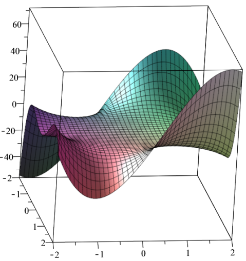
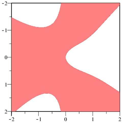
The extent to which derandomization is possible depends on the “complexity” of the sets we allow. If is only given via a black-box membership oracle then no derandomization is possible. So we need to assume an “explicit description” of is given, and in this paper we focus on the case that is the set of points satisfying a polynomial inequality of degree at most (i.e., is the set indicated by a degree- PTF). Thus the case allows halfspaces, the case allows ellipsoids and hyperboloids, etc. For illustrative purposes, Figure 1 shows an example with and , although we generally think of .
One natural approach to this volume-approximation problem is the following: First, define some kind of explicit (nonrandom) finite “grid” of discrete points in ; second, show that the Gaussian volume of any degree- PTF set is closely approximated by the fraction of grid points in . A naive gridding scheme would use at least an exponential-in- number of grid points (even for ); the question is whether we can use a subexponential-in- number of gridpoints, when . Our Theorem 1 provides such a solution; by enumerating all seeds (essentially, taking the support of ), we get an explicit set of just “grid points” that gives a high-quality volume approximation for any degree- polynomial threshold set; this is nontrivial for up to some . Also note that this kind of “PRG solution” is stronger than just being an “volume-approximation” algorithm of the type “given , approximate ”; as it is PRG-based, it gives one fixed, deterministic “grid” that simultaneously works to approximate the volume of all degree- polynomial threshold sets .
Boolean complexity theory.
As mentioned earlier, the problem of PRGs (or deterministic volume approximation) for Gaussian polynomial threshold functions is a special case of the problem of PRGs (or approximate-counting) for Boolean polynomial threshold functions. This, in turn, is a very special case of the problem of derandomization for general Boolean circuits. Recall that the vs. problem is roughly equivalent to asking whether there is a deterministic polynomial-time algorithm that, given the explicit description of a subset in the form of a -gate Boolean circuit computing the indicator function of , computes a -accurate approximation to its “volume”, . Given how far we are from answering this question, the field of pseudorandomness has focused on special classes of circuits, of restricted depth and gate-types; the case of Boolean PTFs corresponds to depth- circuits with a threshold gate on top and AND gates of width at most at the bottom.
1.3 Our key new tool: the Local Hyperconcentration Theorem
For large , the best prior PRG for degree- Gaussian PTFs is Kane’s [Kan11b], which has seed length . In this section we describe the most important new ingredient we introduce to Kane’s framework, which lets us reduce the seed length’s dependence on down to . In the next section we will give an overview of the constructions of [MZ10, MZ13, Kan11b], putting our new tool into context.
We call our main new tool the Local Hyperconcentration Theorem. To explain it, suppose is a degree- polynomial. Since has high degree, it might fluctuate quite wildly near a given point , causing to rapidly switch between in small neighborhoods. However, we might hope that for most points , the value of in a local neighborhood of is almost always within a multiplicative factor of , and hence is almost always of constant sign.
The right definition of a “local neighborhood of ” is to choose a small scale parameter , and then to consider a Gaussian , centered at , with variance in each coordinate.444The factor is included so that when we look at a typical chosen from , the resulting “random point in the neighborhood” also has distribution . Now if , we may say that is (multiplicatively) concentrated in this -local neighborhood of ; and indeed, the second moment method (Chebyshev’s inequality) tells us that almost always has the same sign (namely, the sign of ). The most important ingredient in Kane’s work, [Kan11b, Cor. 10+Lem. 11], establishes this sort of result:
Theorem 2 (The key technical theorem of [Kan11b], simplified).
Let be a degree- polynomial. Provided , with high probability over we have
| (1) |
We may say that Kane shows degree- polynomials have local concentration at scale , almost everywhere. The value ends up becoming the dominant factor in Kane’s PRG’s seed length. At a high level, this is because the PRG has the form , where the ’s are independent random vectors with -wise-independent distributions.
By way of contrast, our new Local Hyperconcentration Theorem (stated in simplified form below) shows local hyperconcentration at scale . For a high level sketch of the proof, see Section 5.1.
Theorem 3 (Simplified Local Hyperconcentration Theorem, see Theorem 47 and Theorem 85).
Let be a degree- polynomial. Provided , with high probability over we have
| (2) |
for any large constant (indeed, for any ).
Remark 4.
The conference version of this paper [OST20] proved a quantitatively weaker version of the Local Hyperconcentration Theorem, showing local hyperconcentration at scale . This led to a seed length of . Subsequently, Kane improved the Local Hyperconcentration Theorem to show local hyperconcentration at scale , which yields the current seed length of . Kane’s proof is given in Appendix B and subsumes Section 5 of this paper. After the initial appearance of this work on the ArXiV [OSTK21] we were informed by R. Meka that he and Z. Kelley had independently and concurrently obtained results similar to the main result of this work [KM21].
We will define “hypervariance” later (see Definition 27); here we only note that it is a stronger notion than variance, in the sense that is always at least as large as for all Whenever the theorem’s conclusion holds for an outcome of the value of in the -local neighborhood of is “hyperconcentrated” (see Lemma 31), meaning that for any large constant ,
The case here is precisely the “concentration” conclusion in the theorem of [Kan11b]. Our hyperconcentration is a stronger conclusion: e.g., taking lets us use the “fourth moment method”, and in fact we’ll eventually use .
To summarize, our theorem has two important improvements over [Kan11b]. First, it shows concentration at a much larger scale, , rather than . This crucially gives us the potential to get our seed’s dependence on to be . This is far from automatic, though, because there are several other places in the [Kan11b] construction that “lose” a factor of . In all but one of these cases555Namely, our “noise insensitivity extension lemma” Lemma 72, where we eliminate a factor of from the analogous result of Kane [Kan11b, Cor. 16]., it’s because in [Kan11b] the variance bound Equation 1 is bootstrapped using the hypercontractivity inequality in order to get control over ’s behavior in various local neighborhoods. This hypercontractive inequality for degree- polynomials inherently loses factors (see Theorem 20). By contrast, since our theorem already establishes the stronger hyperconcentration conclusion Equation 2 (this is the second key improvement, bounding hypervariance rather than variance), we are able to provide argumentation that eliminates all of these factors.
1.4 Overview of the PRG framework we use
We use the same PRG for Gaussian PTFs as in the prior works of Meka–Zuckerman PRG [MZ10, MZ13] and Kane [Kan11a], namely
| (3) |
where the key parameter is a small function of and , where , and where are independent random vectors, each having an -wise independent -dimensional Gaussian distribution. This leads to a seed length of essentially (see Theorem 10), and hence all the effort goes into finding the largest such that Equation 3 -fools degree- Gaussian PTFs.
Here we review the Meka–Zuckerman and Kane works; our own analysis is heavily based on Kane’s framework.
Meka–Zuckerman.
The work of Meka and Zuckerman [MZ10] gave PRGs for degree- Gaussian PTFs with seed length . In fact, they also extended their results to Boolean PTFs, but we do not review that extension here. At a high level, their construction followed a basic two-part paradigm used both in the proof of Central Limit Theorems and in PRG construction: mollification + local low-degree behavior. To explain this, recall that we are trying to design a PRG with
where , with a degree- polynomial. Suppose first that we did not have the discontinuous “” function, but rather we just wanted the above inequality for . In that case, it would suffice for the components of the random vector to be “-wise independent,” and in fact this would achieve . Furthermore, there are standard techniques to produce an appropriate “-wise independent” with seed length , which would be an excellent bound for us.
Of course, when we return to the actual scenario of , the function is not even a polynomial, let alone a low-degree one. The mollification portion of Meka and Zuckerman’s work is to replace the function with a smooth approximator , which is equal to outside some interval . Because the function is scale-invariant ( for ), we may normalize so that its variance is . Then one chooses the parameter . The smooth mollifier will have derivatives of all orders, with th derivative bounded in magnitude by . The replacement of by leads to a mollication error of , essentially due to the well-known anticoncentration bound for degree- Gaussian polynomials due to Carbery and Wright [CW01]: . (Note also that thanks to a trick, this only needs to hold for , and not the pseudorandom .) With the mollifier in place, Meka and Zuckerman can try to bound
Now although is not a polynomial, it is “locally a low-degree polynomial” (say, of degree ), thanks to Taylor’s theorem. The error in this statement scales like the th derivative bound , times the “locality scale”. Thus as long as we substitute -wise independent Gaussians for true Gaussians at a “scale” of , we will not incur more than error. This sort of argumentation allows Meka and Zuckerman to show that the PRG in Equation 3 -fools degree- PTFs with , which leads to their seed length of .
Kane.
To repeat, our PRG analysis closely follows the structure of Kane’s, which we now describe. Kane [Kan11b] shows that the PRG in Equation 3 succeeds with the improved (larger) value of , leading to his seed length of . His “local concentration theorem” (Theorem 2) plays a central role in this, but he still needs to develop a complex framework (which we also employ) in order to complete the analysis.
Kane’s Theorem 2 allows him to begin a new strategy for designing ; rather than mollifying the function and taking as a “black box” random variable, Kane instead mollifies the polynomial itself. Roughly speaking, Kane’s strategy begins by replacing with , where is a smoothed indicator function for the event that Equation 1 holds at . The “with high probability over ” in Kane’s Theorem 2 is in fact probability provided , and this implies that the replacement of by only incurs error . Now we may hope that the construction from Equation 3 will work; roughly, this requires that in a -scale neighborhood of every point , say , the function is essentially determined by low-degree moments of . There are two cases. If is well into the region where is , then is essentially and is essentially constant. Otherwise, if is near the region where is , then by definition is very small. Thus is not varying very much in a neighborhood of , and Taylor’s theorem will tell us that low-degree moments suffice to essentially determine in this neighborhood of .
There are two catches here. First, the use of Taylor’s theorem out to, say, degree forces one to bound not just the expected squared deviation of from in the -neighborhood of ; it requires one to control, say, the th-power deviation. This is where Kane uses the standard hypercontractivity-based fact that higher-power deviations can be controlled by the nd-power deviation (i.e., ) at the expense of losses. Kane is losing such factor anyway, since he takes . (This is one place where our analysis takes advantage of the local hyperconcentration we prove in Theorem 3.)
The second catch is that Taylor’s theorem needs to be applied not just to but to itself. Now is concerned with the variance of in a -neighborhood of . In order to control the Taylor error here, one needs to control the variance of the variance! Kane handles this by further mollifying . He uses a generalization of Theorem 2 to show that at most points , the variance of the variance in the neighborhood of is small. (We must prove a similar generalization of our Local Hyperconcentration Theorem; see Theorem 49.) Thus can be further mollified to at only small loss. Now we have three cases to consider when analyzing ; if is well into the region where is , then the mollified function is essentially on the -neighborhood. Else, the variance of the variance of in the neighborhood is suitably small. Next, if is well into the region where is , then the mollified function is again essentially on the neighborhood; otherwise, the variance of in the neighborhood is suitably small. In this third case, we are again in good shape to apply Taylor to , and …but to handle Taylor error for , we need to introduce another check that the variance of the variance of the variance is small. Indeed, Kane’s final mollifier needs not only this “descending” sequence of checks (that we will picture “vertically”), but for technical reasons needs additional “horizontally proliferating” checks (which, to avoid further lengthening this description, we will not discuss here).
Luckily, all of these proliferating checks eventually “bottom out”. The vertically descending checks bottom out because the “-fold variance” is a polynomial of degree , and hence the -fold variance is constantly . The horizontally proliferating checks may eventually be terminated due to the fact that a degree- polynomial is determined by its values at points. (Actually, one needs a quantitative version of this fact. Kane provides one involving another factor of ; we eliminate this factor in Lemma 72.)
Ultimately, Kane’s mollifier multiplies by “” functions: one needs a generalization of Theorem 2 and another theorem to show that the mollification is close to at almost all points; and, when using Taylor’s theorem at , one needs a -case analysis looking at the “deepest” check (if any) that “fails.” If any check “fails,” then the mollified function is essentially ; otherwise, if they all pass, then in the -neighborhood of , the variance of , and the variance of the variance, and the variance of the variance of the variance, etc., are all suitably small for use in Taylor’s theorem.
2 The high-level structure of our proof
Throughout this paper is a nonzero polynomial of degree at most , and we are interested in the degree- polynomial threshold function . For a given , we determine a small value
| (4) |
and we also let
| (5) |
Our main goal is:
Theorem 5 (Main result: sum of -wise independent Gaussians fools degree- PTFs).
Let be a standard -dimensional Gaussian random vector, and let be independent -wise independent -dimensional Gaussian random vectors. Write
Then
To prove Theorem 5, we will construct a certain function
which is a smoothed indicator function for a collection of events (related to local hyperconcentration of ) that are expected to almost always occur. We then show the following:
Theorem 6 (Mollification error theorem, analogue of Lemma 17 of [Kan11b]).
We then extend the mollifier to take into account the sign of :
Definition 7.
Define by
and define similarly as
The main thing we prove about is the following:
Theorem 8 (One step of the Replacement Method, analogue of Lemma 19 of [Kan11b]).
Fix any , and assume the -valued random vectors are each -wise independent -dimensional Gaussian vectors. Then we have
The analogous statement for also holds.
From this, a “Replacement Method” argument easily yields the following:
Corollary 9.
Proof.
We may view as
where are independent. For , write
so and . Thus by telescoping,
| (6) |
For a fixed , if we write
then
| (7) |
Since and are each -wise independent -dimensional Gaussian vectors, Theorem 8 implies that Putting this into Equation 6 completes the proof. ∎
With the above ingredients in place, Theorem 5 follows almost immediately:
Proof of Theorem 5.
Since pointwise,
where the second inequality is thanks to Corollary 9 and the third is thanks to Theorem 6. The reverse direction, which lower bounds by using , is similar. ∎
Theorem 5 shows that a scaled sum of -wise independent Gaussians fools degree- PTFs, but such a random variable is not quite the desired PRG since perfectly generating even a single Gaussian random variable formally requires infinitely many random bits. However, the following construction of Kane tells us that for fooling degree- Gaussian PTFs, it essentially suffices to find the least such that they are fooled by sums of independent -wise Gaussians; then, one gets an explicit PRG with seed length .
Theorem 10 (Section 6 of [Kan11b]).
Let , . Suppose that for some , degree- Gaussian PTFs are -fooled by , where and are -wise independent -dimensional Gaussians. Then there is an explicit PRG for -fooling degree- -dimensional Gaussian PTFs with seed length
which is simply under the reasonable assumptions that .
As [Kan11b] does not quite explicitly state Theorem 10, we outline a proof in Appendix A for completeness. Theorem 1 follows immediately from Theorem 5 and Theorem 10.
The remaining tasks are to define and prove Theorems 6 and 8. We define in Section 4 and prove Theorem 6 and Theorem 8 in Sections 4.4 and 7 respectively.
3 Probabilistic preliminaries
In this section we introduce notation and collect several probabilistic facts we will use. Throughout, boldface is used to indicate random variables, denotes the standard Gaussian (normal) distribution, and is the associated -dimensional product distribution.
3.1 Bits, Gaussians, and -wise independence
Although this work is mainly concerned with Gaussian random variables, many (but not all) of the tools in it “generalize” to Boolean random variables. In order to illustrate this, we will provide some definitions and notations in this section that work in both cases. However the Boolean results are never strictly needed in this work, and the reader may prefer to ignore them and focus only on the Gaussian case.
The fact that PTFs over Boolean space generalize PTFs over Gaussian space holds because, for large and uniform and independent,
| (8) |
is “close” to having an distribution, and because a degree- polynomial is also a degree- polynomial in the ’s. One sense of “closeness” here is that each may be coupled with a true Gaussian in such a way that except with probability at most .
Definition 11.
Let be a probability distribution on . We say that a random vector on has a -wise independent distribution if each has distribution , and for all choices of indices , the random variables are independent. Examples include being the uniform distribution on (“-wise independent bits”) and the main concern in this paper, being (“-wise independent Gaussians”).
Remark 12.
The main way we use -wise independence is to say that if is -wise independent, is -wise independent, and is a polynomial of degree at most , then .
3.2 Polynomial expansions
We recall standard facts and notation from analysis of Boolean functions and Hermite polynomials; see, e.g., [O’D14] for a reference, and in particular [O’D14, Ch. 11.2] for Hermite analysis.
Every function can be represented by a multilinear polynomial,
where each and we use the standard multi-index notation and . In “Gaussian space” the only functions we will ever analyze are polynomials; every degree- polynomial can be written in Hermite polynomial decomposition as
where each , and the multivariate Hermite polynomial polynomial is given by , where is a normalized version of the univariate degree- “probabilists’ Hermite polynomial” . The multivariate Hermite polynomials are orthonormal under . Also, in the notation of Equation 8,
| (9) |
Let denote either an -variate Boolean or Gaussian polynomial. We use standard notation for its mean (that is, for in the former case, in the latter), for its -norm (), and for its variance. It holds that
We write for , and similarly write and . We also write for the “weight of below level ”, and similarly write and .
3.3 Noise and zooms
A basic fact about Gaussians is that if are independent and , then is also distributed as . In this work, typically denotes a “small” quantity; for fixed we view as a “-noisy” version of , and we view changing a polynomial ’s input from to as “zooming into at with scale ”. We make a precise definition:
Definition 13.
For an -variate Gaussian polynomial, , and , we define the function by
The function is a polynomial in of the same degree as , and we (nonstandardly) refer to it as the -zoom of at .
Remark 14.
Referring again to Equation 8, one may verify that a -zoom of at a random is the Gaussian analogue of a standard Boolean concept: a random restriction of a function at , meaning a subfunction obtained by proceeding through each coordinate , and either fixing the th input to be with probability , or else leaving it unfixed (“free”) with probability .
The fact that random restrictions of a Boolean function interact well with its polynomial expansion is well known; e.g. [O’D14, Prop. 4.17] gives a formula for the expected square of any Fourier coefficient of a Boolean function under a random restriction. Carefully taking the “Gaussian special case” of this (using Equation 9) yields the below analogue for random zooms. For completeness, we give a self-contained proof of this analogue in Appendix A.
Proposition 15.
For a polynomial, , and ,
where denotes an -dimensional random vector with independent components, the th of which is distributed as the binomial random variable .
Summing the above proposition over all multi-indices of a given weight immediately yields the following useful corollary:
Corollary 16.
For a polynomial, , and ,
3.4 Noise operator and hypercontractivity
Considering the mean of the zoom of a polynomial leads to the “Gaussian noise” (or “Ornstein–Uhlenbeck”) operator (see, e.g., [O’D14, Def. 11.12]):
Definition 17.
Given , the operator acts on Gaussian polynomials via
It is well known that acts diagonally in the Hermite polynomial basis :
| (10) |
In particular, if is a degree- polynomial, so too is .
We may also write for the analogous Boolean noise operator (more usually denoted , see [O’D14, Def. 2.46]), definable for either through Equation 10, or by stipulating that is the mean of a random restriction of at with -probability of fixing a coordinate.
Finally, somewhat unusually, we will need to extend the definition of to , which we can do via the formula Equation 10; equivalently, by stipulating that . For this operator no longer has a “probabilistic interpretation”, but it still maps degree- polynomials to degree- polynomials.
Remark 18.
We will several times use the “semi-group property”, , which is immediate from Equation 10.
At one point in our analysis we will also need the notion of Gaussian noise stability:
Definition 19.
Hypercontractivity.
A nontrivial and highly useful property of the Boolean/Gaussian noise operator is hypercontractivity (see, e.g., [O’D14, Secs. 9.2, 11.1]):
Theorem 20 (-hypercontractive inequality).
Let be a Gaussian or Boolean polynomial. Then holds for any .
Hypercontractivity has the following consequences (see [O’D14, Thms. 9.22, 9.23]):
Theorem 21.
Let be a Gaussian or Boolean polynomial of degree at most . Then .
Theorem 22.
Let be a Gaussian or Boolean polynomial of degree at most . Then for any ,
3.5 Hyperconcentration: our key tool
The ideas in this section, though technically standard, are part of the conceptual contribution of this work.
Very often we will need to show that a random variable is tightly concentrated around its mean in a multiplicative sense. Let us start with some notation.
Notation 23.
We use the following notation to denote that two reals are multiplicatively close: For ,
Note that this condition is indeed symmetric in and . We extend the notation to all by stipulating that if: and the above condition holds; or, .
Given a real random variable with mean , a standard way to show that with high probability is to first establish and then use Chebyshev’s inequality. When this holds we informally say that concentrates around its mean. In this work, a crucial concept will be improving this concentration using higher norms.
Definition 24.
Let and be real numbers. We say a real random variable with mean is -hyperconcentrated if
The utility of this definition is that it gives an improvement to the Chebyshev inequality:
Proposition 25.
Suppose with mean is -hyperconcentrated. Then for any , except with probability at most we have (and in particular if ).
Proof.
Apply Markov’s inequality to the random variable . ∎
We’ll also need the following simple consequence of hyperconcentration:
Lemma 26.
Suppose is an -valued random vector with -hyperconcentrated components, and write . Then for any multi-index with ,
Proof.
We have
where the first inequality is from Hölder’s inequality and the second is from Definition 24. ∎
The random variables we’ll show hyperconcentration for will be Gaussian polynomials. We will do this by bounding a quantity that we term their “hypervariance”, and that plays a central role in our work:
Definition 27.
Let be a Gaussian or Boolean polynomial. Then for , we define the -hypervariance of to be
(For , this reduces to the usual variance of .)
Lemma 28.
Let be a Gaussian or Boolean polynomial. Write and assume . Then the random variable is -hyperconcentrated.
Proof.
Writing , our hypothesis is that . By hypercontractivity, we have . Thus , as needed. ∎
The hypothesis in Lemma 28, that ’s hypervariance is small compared to its squared-mean, will be an important one for us. It is essentially the same as the hypothesis that ’s hypervariance is small compared to its squared--norm (since squared--norm equals squared-mean plus variance, and hypervariance is at least variance for all ). It will be slightly more convenient in our Local Hypervariance Theorem to work with the latter hypothesis, so we codify it here and establish the analogue of Lemma 28.
Definition 29.
Let be a Gaussian or Boolean polynomial, and let . We say that is -attenuated if .
Remark 30.
Intuitively, a polynomial is attenuated if for each , the amount of Hermite weight it has at level is “very small” compared with the total Hermite weight (squared 2-norm) of . Crucially, the precise quantitative definition of “very small” in the preceding sentence depends on the weight level , and gets exponentially stronger (smaller) as gets larger. An intuition which may possibly be helpful is to think of an attenuated polynomial as a polynomial which is “morally constant” over Gaussian space.
Returning to hyperconcentration, we have the following:
Lemma 31.
Let be a Gaussian or Boolean polynomial that is -attenuated, with and . Then the random variable is -hyperconcentrated.
Proof.
Using the notation and again, and starting with the -attenuation assumption, we have
where the last step used and . But this is equivalent to , so the result follows from Lemma 28. ∎
Combining this with Lemma 31 and Proposition 25 yields the following useful result, which informally says that “attenuated polynomials are very likely to take values multiplicatively close to their means”:
Proposition 32.
Let be a Gaussian or Boolean polynomial that is -attenuated, with and . Write . Then assuming , we have except with probability at most .
3.6 Special properties of Gaussian random variables
All of the results in this section so far have applied equally well to Gaussian or Boolean polynomials. We now give the two results we will use that are specific just to Gaussian polynomials. The first is a well known result of Carbery and Wright [CW01] on anticoncentration (see e.g. [Kan11b, Lem. 23], [O’D14, Sec. 11.6]):
Theorem 33 (Gaussian Carbery–Wright).
There is a univeral constant such that for any degree- polynomial and any ,
The second Gaussian-specific result we use is a key lemma from Kane’s work [Kan11b, Lemma 9]. This lemma was the essential ingredient he used to prove his “local concentration” result Theorem 2. At first glance, it may look much stronger than Theorem 2, because it gives a nontrivial kind of concentration result even for as large as . However the concentration one gets in (almost all) local neighborhoods is somewhat weak: one gets that ’s values are with high probability near a specific value, but this is not enough to even conclude that is small compared to that value. Kane uses hypercontractivity to bootstrap this to control over the variance when he obtains Theorem 2, and this loses a factor. When we employ Lemma 34 below, we will already be working with hyperconcentrated functions, which means we will not lose much when similarly bootstrapping.
Lemma 34.
([Kan11b, Lemma 9] with parameters renamed.) Let be a degree- polynomial and let . Then for independent, except with probability we have
(provided is small enough that ).
Kane’s proof of this lemma (seemingly) crucially relies on the rotational invariance of -dimensional Gaussians.
4 Defining
The definition of involves a collection of “statistics” of the polynomial . Each statistic will be a certain nonnegative polynomial , defined in terms of , of degree at most .
The definition also involves a collection MollifierChecks of “mollifier checks”. Each mollifier check will consist of two ingredients:
| (11) |
for some statistics and some nonnegative value , and where is a “softness” parameter. The intuitive meaning of Check applied at a point is that it is “softly” checking that , up to a multiplicative factor of roughly . More precisely:
Definition 35.
Let be a smooth function satisfying
and which is such that for all , the magnitude of ’s -th derivative is everywhere bounded by . (This is easily achieved by standard constructions such as taking to be a suitable polynomial of degree on the interval ) Also, given a mollifier check as in (11), define
by
| (12) |
where we take . We remark that
The function is the product of all the mollifier checks:
Definition 36.
To complete the definition of we need to: (i) define the statistics in ; and, (ii) define the collection MollifierChecks of mollifier checks. We do each of these in turn below.
4.1 The statistics in
4.1.1 Noisy derivatives of amplified polynomials
Now we arrive at a novel definition in this work which plays a key role in our results. We will make extensive use of the following notion, which can be thought of as a sort of “noisy derivative of the -amplified version of at in directions and .” This is a variant of one of the key definitions of [Kan11b] (the second definition in Section 3 of that paper) but with the crucial difference that now we consider the “-amplified” version of in place of just itself as was the case in the corresponding definition in [Kan11b]:
Definition 37.
Given two vectors , define the operator on polynomials via
We remark that is parenthesized as .
The following is easily verified:
Fact 38.
If is a polynomial of degree at most , then for every , the function is a polynomial of degree at most .
The following simple but crucial fact connects the derivative notion from Definition 37 to the hypervariance notion from Definition 27:
Fact 39.
For fixed and independent -dimensional Gaussians , we have that
Proof.
The left-hand side is equal to
| (since for ) | |||
where the penultimate equality is by orthonormality of the Hermite polynomials and independence of . ∎
4.1.2 The statistics in
Fix a parameter
| (13) |
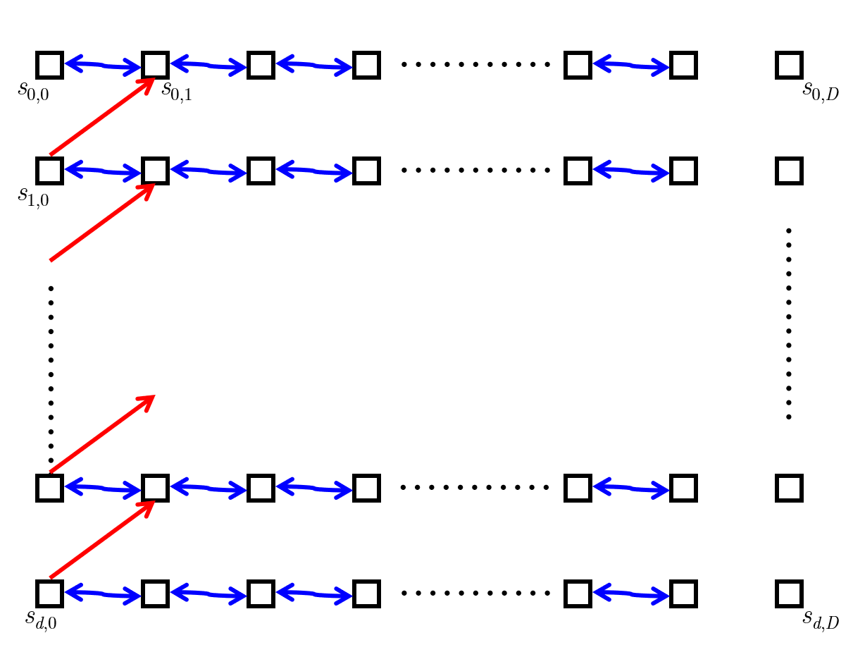
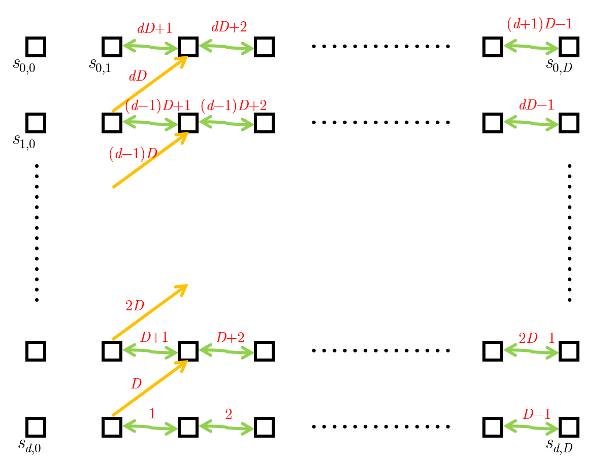
where is a parameter we will set later. (See Equation 33; it will in fact be an absolute constant.) We can now define the set of statistics, . Each statistic is doubly indexed by a pair of natural numbers; there are many statistics, where
| (14) |
It is convenient for us to view the elements of as being arranged in a grid where the -th statistic is in row and column (we will often use terminology of this sort). We remark that our statistic will closely correspond to the functions called in [Kan11b] (), except that as mentioned we use amplified noisy derivatives where Kane just had noisy derivatives.
All statistics are defined in terms of the underlying degree- polynomial . We first define the 0th column of statistics:
Definition 40 (0th column of statistics).
For , we define
where are independent.
Remark 41.
By 38, is a constant function and is identically zero; this is why we consider only for .
For technical reasons, we will also need to use slight variants of the statistics , which correspond to taking an average over mildly noisy versions of the input:
Definition 42 (The remaining statistics).
For and we define by
Remark 43.
Using the semigroup property, we have that
This completes the formal definition of the statistics in ; however, it will be very useful for us to view the statistics from a different perspective based on distributions of polynomials. We introduce this perspective in the next subsection.
4.2 A distributional view on the statistics
For the sake of probabilistic technicalities, we will need to define a notion of a distribution of polynomials being “nice”:
Definition 44.
We say that a distribution of -variable polynomials of degree at most is nice if
-
•
is the normal distribution for some natural number , and
-
•
for each in the support of , the coefficients of are polynomials of degree at most in
It will be convenient for us to view the statistics as averages of squares of polynomials drawn from various nice distributions. To do this, we inductively define a grid of nice distributions of polynomials as follows. The base distribution, is just the probability distribution with a single outcome, namely the polynomial . (Note that this corresponds to a nice distribution with ) Next, we inductively define the distributions as follows:
-
•
To make a draw from , where : First draw . Then draw . Then output the polynomial .
The following “operator notation” for zooms (local to this section and Section 8.3) will be convenient: for a polynomial and a vector , we define the notation
| (15) |
With the distributions of polynomials defined as above, we inductively define the distributions , where as follows:
-
•
To make a draw from , where : First draw . Then draw . Then output the polynomial .
It is immediate from these definitions that each is a nice distribution of polynomials of degree at most . It is also immediate, comparing the above definition against Definition 40 and Definition 42, that for each and each we have that
| (16) |
Finally, it is straightforward to check from these definitions (using also 39) that
| (17) |
These characterizations will be useful when we analyze the statistics later.
4.3 Defining the mollifier checks
Intuition. In this subsection we define the collection MollifierChecks of mollifier checks. Before formally defining these checks, we give some useful intuition concerning them. We will show in Section 4.4 that except with very small failure probability over , the statistics satisfy the following properties, where are suitable small parameters:
-
1.
Local hyperconcentration: For each ,
(18) -
2.
Insensitivity under noise: For each ,
(19)
The parameter settings we require will turn out to be the following:
| (20) |
where is a suitably large absolute constant and is a constant that will be set later in Equation 33 (for now, the most important thing to notice is that since , the exponent on above is strictly greater than ).
The mollifier checks are designed precisely to check that the above properties Equations 18 and 19 actually hold at , and thus Theorem 6 corresponds to the fact that these properties hold with high probability for a random .
With the above intuition in place, we proceed to define the mollifier checks that check for each of the above types of properties (1) and (2). Please see below for a figure depicting the mollifier checks and the grid of statistics.
4.3.1 Checking local hyperconcentration
For each , MollifierChecks contains a check corresponding to Equation 18. The “inequality” portion of the check is
and the “softness” parameter of the check is ; so for this check Check in the associated “soft check” is
| (21) |
We refer to these elements of MollifierChecks as “anticoncentration checks” or (recalling the grid) as “diagonal checks.”
4.3.2 Checking insensitivity under noise
For each MollifierChecks contains a pair of checks corresponding to Equation 19. The “inequality” portion of the first (respectively, second) check of the pair is
and the “softness” parameter of each of these checks is . So for these two elements of MollifierChecks the associated “soft checks” are
| (22) | ||||
| (23) |
We refer to these checks as “noise-insensitivity checks” or as “horizontal checks.”
This concludes the definition of MollifierChecks, so recalling Definition 36 the definition of is now complete. We turn to proving Theorem 6.
4.4 Breaking down the mollification error for the proof of Theorem 6
Recalling the definition of MollifierChecks from Section 4.3, the approach to proving Theorem 6 is clear. We will show that each of the local hyperconcentration (diagonal) checks passes “with room to spare” with high probability over , and that likewise each of the noise-insensitivity (horizontal) checks passes with room to spare with high probability over . The two theorems stated below give the desired bounds:
Theorem 45 (Local hyperconcentration, rough analogue of Corollary 10 of [Kan11b]).
For each , except with probability at most over , Equation 18 holds, i.e.
Theorem 46 (Noise-insensitivity, analogue of Lemma 11 of [Kan11b]).
For each and except with probability at most over , Equation 19 holds, i.e.
-
Proof of Theorem 6 using Theorem 45 and Theorem 46..
By a union bound over failure probabilities, we have that with probability at least Equation 18 holds for all and Equation 19 holds for all . If Equation 18 holds for a given then and the diagonal check Equation 21 evaluates to 1. If Equation 19 holds for a given then and the horizontal check Equation 22 evaluates to 1, and similarly and the horizontal check Equation 23 evaluates to 1. ∎
It remains to prove Theorems 45 and 46.
5 Local hyperconcentration: Proof of Theorem 45
In this section we present the key new ingredient underlying our main result, the Local Hyperconcentration Theorem for degree- polynomials. As alluded to in the Introduction, this result says that with high probability over a Gaussian the -zoom of a degree- polynomial at (i.e. the polynomial ) is attenuated — intuitively, it is “very close to a constant polynomial”. We refer to this result as a “local hyperconcentration theorem” since by Lemma 31 attenuation of implies that the random variable (for ) is hyperconcentrated; this property will play a crucial role in our later technical arguments.
For technical reasons related to the definition of our statistics (essentially because each statistic is an average of polynomials — recall Section 4.2), the actual statement we will need is one that is about a distribution of polynomials rather than a single polynomial. However, for clarity of exposition we first state the “one-polynomial” version of the original local hyperconcentration theorem from [OST20] below:
Theorem 47 (Local hyperconcentration theorem for a single polynomial).
Let be a polynomial of degree at most . Fix parameters ,, , and assume
(where is a certain universal constant). Then for , except with probability at most we have that the randomly zoomed polynomial is -attenuated; i.e.,
Another way to phrase the conclusion is that for , except with probability we have that is such that
Notice that the dependencies here on and are “correct” in the sense that if one intuitively thinks of as “infinitesimal”, we expect that will have weight at level , negligible weight above level , and the definition of multiplies this level- weight by . The “error factor” in this result, with , essentially becomes our final seed length (divided by ).
Because of the need to analyze the statistics introduced in Section 4.1.2, we will often need to work with a distribution over polynomials rather than a single polynomial. We therefore introduce the following generalization of Definition 50, which captures the notion of a distribution over polynomials being attenuated on average:
Definition 48 (Nice distribution of polynomials is attenuated on average).
Let be a nice (in the sense of Section 4.2) distribution of polynomials over . For and , we say that the distribution is -attenuated on average if
The actual main result we prove in this section is Theorem 49, which generalizes Theorem 47 to a nice distribution of polynomials and is the original local hyperconcentration theorem from [OST20]:
Theorem 49 (Local hyperconcentration theorem for a nice distribution of polynomials).
Let be a nice (in the sense of Section 4.2) distribution of degree- polynomials. Fix parameters , , , and assume
| (24) |
(where is a certain universal constant). Then for , except with probability at most we have that the distribution is -attenuated on average; i.e.,
In Appendix B an improved version of Theorem 49, namely Theorem 85, is proved, which only requires an upper bound on of . Theorem 45 follows from Theorem 85 directly by setting parameters as follows:
-
Proof of Theorem 45 using Theorem 85.
We instantiate Theorem 85 with its nice distribution “” being , its “” parameter being set to defined in Equation 13, its “” parameter being , its “” parameter being , and its “” parameter being . Recalling Equation 16 and Equation 17 we have
Recalling the settings of and from Equation 4 and Equation 20, we see that the bound required in Equation 24 indeed holds, and so we can apply Theorem 85, and its conclusion gives precisely the desired conclusion of Theorem 45. ∎
In the rest of this section we prove Theorem 49. We first explain the high-level structure of the argument in Section 5.1 and then give the formal proof in the rest of the section.
5.1 A useful definition, and the high-level argument underlying Theorem 49
Before we can give the high level idea of the proof of Theorem 49 we need a refined notion of a polynomial being attenuated:
Definition 50 (Attenuated polynomial, refined notion).
Let be a polynomial of degree at most For , , and , we say that the polynomial is -attenuated if
| (25) |
Similarly, if is a nice (in the sense of Section 4.2) distribution of polynomials over , we say that the distribution is -attenuated on average if
Note that being -attenuated is the same as being -attenuated as defined earlier (see Definition 29), and likewise for (see Definition 48).
With this refined notion of attenuation in hand we can explain the high level idea of our local hyperconcentration theorem. For ease of exposition, below we sketch the underlying ideas in the “one-polynomial” setting of Theorem 47 (the same ideas drive the proof of Theorem 49).
So, we are given a degree- polynomial and the goal is to argue that with high probability over a random point , the polynomial is -attenuated, i.e. -attenuated. A simple but crucial insight pointing the way is that random zooms compose: in more detail, if are two noise rates and are two independent random variables, then the distribution of the composed random zoom is identical to the distribution of where . With this in mind, it is natural to view a random zoom at the small noise rate as a “strong” random zoom which is obtained by composing a sequence of many “weaker” random zooms at larger noise rates.666The idea of decomposing a “strong”random zoom into multiple “weak” random zooms is due to Avi Wigderson. If we can prove that a “weak” random zoom with high probability causes a -attenuated polynomial to become -attenuated, then since any degree- polynomial is trivially -attenuated, a simple union bound over many applications of this “one-stage” result yields the desired random zoom lemma for . This is precisely the high-level structure of our argument; see Theorem 54 for a formal statement of the one-stage result in the more general setting of a nice distribution of polynomials.
We proceed to give intuition for the proof of the one-stage result. In this setting we are now given which is a -attenuated polynomial; intuitively this means that the amount of Hermite weight it has at levels is very small compared to the total Hermite weight of at all levels . We must argue that with high probability over , after a random zoom at the polynomial is -attenuated, i.e. the amount of Hermite weight has at levels is very small relative to the total Hermite weight of at levels . This is naturally done via a two part argument. The first part is to argue two-norm retention: this amounts to showing that with high probability over , the squared two-norm of does not become too small relative to the squared two-norm of . The argument for this is based on the Carbery–Wright anticoncentration bound (Theorem 33) and the tail bound for Gaussian polynomials (Theorem 22); see Section 5.2 for a precise statement and proof of this part. The second part is to argue attrition of the high-degree Hermite weight: this amounts to showing that with high probability after a random zoom, the amount of Hermite weight at levels becomes very small relative to the squared two-norm of . The argument for this is based on Corollary 16 and Markov’s inequality; see Section 5.3 for a precise statement and proof.
5.2 First part of the proof of the one-stage local hyperconcentration theorem: Retention
The main result of this section is Lemma 52. Its proof uses the following proposition:
Proposition 51.
Let be a nice distribution of polynomials of degree at most . Then for , except with probability at most we have
Proof.
Let We observe that is a nonnegative degree- polynomial with mean
The claimed result now follows immediately from the Carbery–Wright anticoncentration bound Theorem 33 applied to , since . ∎
One way to think of the nice distribution of degree- polynomials in Proposition 51 is that it is “-attenuated on average.” Lemma 52 relaxes this requirement and shows that a similar result holds for a nice distribution that is -attenuated on average for a modestly large .
Lemma 52.
Let be a nice distribution of polynomials that is -attenuated on average for some . Fix a parameter . Then for except with probability at most we have
provided that (for a certain universal constant )
Proof.
We introduce the notation and for , so . We may assume without loss of generality that , or equivalently, . Since is -attenuated on average, we have that
| (26) | ||||
We may deduce that
where the latter inequality holds assuming is large enough. From Proposition 51, we conclude that
| (27) |
where is a universal (large) constant. Our goal will be to establish the following: for all ,
| (28) |
Before establishing Equation 28, we show how it yields the conclusion of the lemma. Given Equations 27 and 28, summing over and taking a union bound, we get that except with probability at most over ,
| (29) |
The triangle inequality easily gives that for functions , we have that
Applying this (for each outcome of ) with and , by Equation 29 we get that
from which we get (using ) that
which is the conclusion of the lemma since .
Thus it remains to establish Equation 28. To do this, write for brevity, and note that is a nonnegative polynomial of degree at most . Similar to the proof of Proposition 51, we have that
and by Equation 26 we have that . Now using Theorem 21 we get that and therefore (using Theorem 22, with its “” set to ) we get that
for any choice of . We will select , so that the preceding inequality aligns with Equation 28; recalling the bound on , this choice of is indeed at least provided is taken at least . Also taking sufficiently large in our assumption on , it is not hard to arrange for the error probability above to be at most . Thus Equation 28 is established and the proof of Lemma 52 is complete. ∎
It is interesting to observe that both the results of this section, Proposition 51 and Lemma 52, hold with no dependence on the value of
5.3 Second part of the proof of the one-stage local hyperconcentration theorem: Attrition
The attrition result we establish in this subsection, Lemma 53, is a fairly direct consequence of Corollary 16. (Note that Lemma 53 does not require that the nice distribution be attenuated on average — it holds for any nice distribution of degree- polynomials.)
Lemma 53.
Let be a nice distribution of polynomials of degree at most . Fix parameters , , , , let be a sufficiently small constant, and assume . Then for ,
holds except with probability at most .
Proof.
The expectation of the left-hand side is
| (Corollary 16) | ||||
| (if small enough) | ||||
| (by the bound on ) | ||||
The result now follows by Markov’s inequality. ∎
5.4 Putting the pieces together: Proof of the local hyperconcentration theorem
Combining Lemma 52 and Lemma 53 (with the “” and “” parameters satisfying , and adjusting constants), we may deduce the following, which is our “one-stage local hyperconcentration theorem:”
Theorem 54 (One-stage local hyperconcentration theorem).
Let be a nice distribution of polynomials of degree at most , and assume the distribution is -attenuated on average for some . Fix parameters , , , and assume
for a suitably large universal constant . Then except with probability at most over , the distribution is -attenuated on average.
Note that a nice distribution of degree- polynomials is -attenuated on average for any . We can take and perform a first application of Theorem 54 on with its parameter set to and its parameter set to 1, and infer that except with failure probability at most the distribution is -attenuated on average. Repeating this a total of times, with each repetition having its parameter set to , its parameter set to (for simplicity), and its parameter set to , we get that except with probability , the distribution is -attenuated on average, where . Finally, we perform one last application of Theorem 54 with its parameter set to 1, its parameter set to , its parameter set to the “” of Theorem 49, and its parameter set to and its parameter set to . We get the conclusion of Theorem 49 as stated at the beginning of this section, and the proof of the local hyperconcentration theorem is complete.∎
6 Noise insensitivity of the statistics: Proof of Theorem 46
Remark 55.
Before entering into the proof, we note that Theorem 46 is analogous to Lemma 11 of [Kan11b], which shows that for every for most , the -th statistic at is multiplicatively close to the -th statistic at . [Kan11b]’s proof of Lemma 11 uses his Lemma 34 (i.e., [Kan11b, Lem. 9]) together with hypercontractivity, but as we discussed earlier, this incurs a factor.
Our arguments in this section also use Lemma 9 of [Kan11b], but they additionally use our Local Hyperconcentration Theorem and our notions of attenuation and hyperconcentration (specifically Proposition 32). These new ingredients let us avoid the factor which is incurred at this point in the [Kan11b] argument.
We proceed with the proof of Theorem 46. We begin by recording a simple corollary of Lemma 34:
Corollary 56.
Next, combining Theorem 85 with Proposition 32, we derive the following:
Proposition 57.
Let be a degree- polynomial and let , , . Say that is “well-behaved” if
Then is well-behaved except with probability , provided
Given some , let us take
It follows that if is both good and well-behaved, then
Since , the only way this can happens is that . Thus the above two propositions imply that except with probability at most over , we have
provided . Selecting and , we conclude (recalling that ) that
Applying this with completes the proof of Theorem 46. ∎
7 Proof of Theorem 8: one step of the Replacement Method
In this section we define a collection of “analysis checks,” which are inequalities among the statistics, and explain the high-level structure of the proof of Theorem 8. The analysis checks play a crucial role in the proof of Theorem 8: as we explain in Section 7.2, two very different arguments (corresponding to Lemma 59 and Lemma 60) are used to establish the conclusion of Theorem 8 at a given , depending on whether or not all of the analysis checks hold at that .
7.1 Analysis checks
In this subsection we define our set of “analysis checks,” which we denote AnalysisChecks. They are related to, but somewhat different from, the mollifier checks MollifierChecks that were used to define the mollifier in Section 4.
One difference between the analysis checks and the mollifier checks is that since the mollifier checks needed to be “actually encoded into the mollifier,” each one needed to consist of both an inequality Ineq among the statistics and a “softness” parameter . In contrast, the analysis checks only play a role in our analysis and do not need to be encoded in the mollifier, and for this reason each analysis check consists only of an inequality Ineq among the statistics. Other than this, the difference between the analysis checks and mollifier checks is that the analysis checks essentially correspond to the mollifier checks “shifted right by one in the grid.”
Below we describe the analysis checks in more detail and highlight the difference between them and the mollifier checks.
Definition 58.
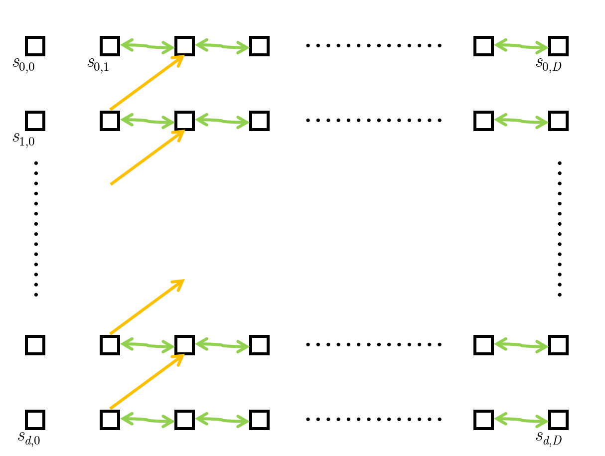
The set AnalysisChecks contains the following checks (inequalities among statistics):
-
•
The horizontal checks: for every , for every , we check that
(30) (so inequalities in total for the horizontal checks), where we set
(31) (Looking ahead, we note that this choice of is less than the upper bound on imposed by the noise insensitivity extension lemma, Lemma 72, which is the main result of Section 9.) Note also that while the mollifier checks defined in Section 4.3 check against for , here we are checking against for . Thus these checks correspond precisely to the mollifier’s noise-insensitivity checks, but “shifted to the right by one.”
-
•
The diagonal checks: for just the st column (note, not the th column), for all we check that
(32) (so diagonal checks in total). Note that while the strong anticoncentration checks defined in Section 4.3 check against , here we are checking against So similar to the previous bullet, these checks correspond precisely to the mollifier’s strong anticoncentration checks, but again “shifted to the right by one.”
Below we give an illustration of the analysis checks.
7.2 High-level structure of the proof of Theorem 8
Let us define the following small integer parameter,
| (33) |
which will be the degree out to which we use Taylor’s theorem.
Theorem 8 will be an immediate consequence of the below two lemmas, since by Equation 20, Equation 5 and Equation 4 we have that :
Lemma 59 (If analysis checks all pass, -wise moments determine mollifier’s value).
Suppose that is such that all of the checks in AnalysisChecks hold at , and that the random vector is a -wise independent -dimensional Gaussian. Then is determined up to an additive .
Lemma 60 (If an analysis check fails, mollifier is close to zero).
Suppose that is such that some check in AnalysisChecks does not hold at , and that the random vector is a -wise independent -dimensional Gaussian. Then .
As we will see in the following sections, two very different arguments are used to prove Lemma 59 and Lemma 60. Lemma 59, which corresponds to the case in which is such that all of the analysis checks pass, is based on a Taylor’s theorem argument. In contrast, Lemma 60, which corresponds to the case in which is such that some analysis check fails, employs a delicate argument, which takes advantage of the careful way that the analysis checks are structured vis-a-vis the mollifier checks, to argue that in this case almost all outcomes of result in .
Before we can enter into the proofs of Lemma 59 and Lemma 60, there are several intermediate technical results which will be used in both proofs which we need to establish. We state and prove these technical results in Section 8 and Section 9, and prove Lemma 60 and Lemma 59 in Section 10 and Section 11 respectively.
8 Bounding the hypervariance of a statistic by its “neighbors”
The main goal of this section is to prove the following technical result which will be needed for our analysis. For every , it gives an upper bound on the hypervariance of the zoom-at- of our -th statistic in terms of the values of some “nearby” statistics:
Theorem 61 (Bounding hypervariance of zooms (analogue of Proposition 12 of [Kan11b])).
For all all , and all , it holds that
We stress that Theorem 61 holds for every input . This is important because Theorem 61 will be used to prove Theorem 8, and in that setting we are dealing with an arbitrary .
Remark 62.
Theorem 61 is analogous to Proposition 12 of [Kan11b], which upper bounds the variance of the zoom-at- of [Kan11b]’s -th statistic in terms of the values of the -th and -th statistics. However, there is a factor of present in the bound of [Kan11b] (again because of hypercontractivity) which as always is incompatible with our goal of achieving an overall quasipolynomial rather than exponential dependence on .
Before entering into the proof of Theorem 61, we record some corollaries and related results which we will use in Sections 10 and 11. Fix any , let denote a -wise independent -dimensional Gaussian random vector, and let us write to denote . Let us also introduce the notation
We first record the following:
Fact 63.
For all and all , we have that
| (34) |
Proof.
We have
where the first equality is Definition 42, the second is because is a polynomial of degree at most and , and the last is by the non-negativity of ∎
Next, as a corollary of Theorem 61 we have the following:
Corollary 64.
For all and all ,
| (35) |
(where we interpret ).
Proof.
We begin by noting that if , then (recalling Remark 43 and Definition 40) it must be the case that is the constant-0 polynomial and hence is also zero; in this case is the identically-0 random variable, which is certainly -hyperconcentrated. Hence we subsequently assume that
By Theorem 61, we have that
| (36) |
We apply Lemma 28 to the function , observing that the “” of Lemma 28 is and hence that Equation 36 lets us take the “” of Lemma 28 to be Since , Lemma 28 thus gives that (for ) the random variable is -hyperconcentrated. Since is a polynomial of degree at most and , the -th moments of and of are identical (recall Remark 12). Now by the definition of hyperconcentration of a random variable we get that Equation 35 holds as desired.∎
8.1 Proof of Theorem 61
Theorem 61 is proved using the following two results. We note that each of these results holds in a fairly general setting: in Lemma 65 can be any nice distribution of polynomials, and in fact both lemmas hold for polynomials over either Boolean space or Gaussian space (it will be clear from the proofs that they go through essentially unchanged in the Boolean context).
Lemma 65.
Let be a nice distribution over polynomials (as defined in Section 4.2) over Gaussian space. Then for , we have
Lemma 66.
777We note at this point that [Kan11b] appears to have a gap in the proof of its Proposition 12. Specifically, it is not true that the second equality following “Notice that” in that proof holds true (roughly speaking, because the derivative operator and the noise operator of [Kan11b] do not in general commute, as can be verified by considering the polynomial . The raison d’être of our Lemma 66 is to fill this gap.For all and all , and all , we have
-
Proof of Theorem 61 using Lemma 65 and Lemma 66.
We instantiate Lemma 65 by taking the nice distribution to be With this choice corresponds to (by Equation 16), and corresponds to (by Equation 17). The final quantity on the right-hand side of Lemma 65, , corresponds to , so from Lemma 65 we get that
(Lemma 66) and the proof of Theorem 61 is complete. ∎
8.2 Proof of Lemma 65
Our main goal in this section is to prove the following:
Lemma 67.
Let be a nice distribution over polynomials (as defined in Section 4.2) over Gaussian space. Define the function
Then if , we have
where .
Lemma 65 follows from Lemma 67 since , is an increasing function of for all , and
| (Equation 10 and Plancherel) | ||||
| (Definition 27 and choice of ) |
We will use the following lemma in the proof of Lemma 67:
Lemma 68.
Given any polynomial and any , we have
Proof.
Let us write where and . Since , we have that
and thus
where the latter inequality is by Cauchy–Schwarz. By -hypercontractivity (recalling Theorem 20), we have that
and similarly
where the last equality holds because and are orthogonal. Thus we have shown that
∎
-
Proof of Lemma 67.
We have
(Definition 27) (Theorem 21) (definition of one-norm) Next we observe that
where the second equality holds because the operator which maps to (i.e. projecting to the -th Wiener chaos) is a linear operator, and the inequality is the triangle inequality. Continuing the above, we deduce that
(monotonicity of norms) (as for any ) Now we apply Lemma 68 to each , which lets us continue as follows:
(Cauchy–Schwarz) (definition of ) completing the proof. ∎
8.3 Proof of Lemma 66
We begin by re-expressing the right-hand side of Lemma 66:
| (37) |
where the last equality is by the definition of in terms of .
We similarly re-express the left-hand side of Lemma 66:
| (38) |
where the last equality is by the semigroup property / Remark 43. Comparing Equation 37 and Equation 38, Lemma 66 is an immediate consequence of Proposition 69, stated and proved below (setting its parameter to be ), which states that the desired inequality holds “outcome by outcome” for outcomes of
Proposition 69.
For all (and in particular ), for every polynomial , and every , we have that
| (39) |
Since the proof of Proposition 69 is somewhat involved we explain the high-level idea underlying it before entering into the technical details. When the quantities in Equation 39 are somewhat difficult to work with since the Gaussian noise operator , which is involved in the definition of the operator, does not admit a convenient probabilistic interpretation (recall that for the definition of is through Equation 10). The proof of Proposition 69 takes advantage of the fact that for , the quantity corresponding to the left-hand side of Equation 39 does have a natural probabilistic interpretation, and likewise for the quantity corresponding to the right-hand side. These probabilistic interpretations let us give tractable expressions for each of the two quantities, and as we will see, it is evident from these expressions that the corresponding quantities correspond to polynomials in of degree at most . These polynomials can then be analyzed to show that the left-hand side is indeed at most the right-hand side for all , as asserted by the proposition.
-
Proof of Proposition 69.
We define the function to be
(40) and the function to be
(41) Let
The following two claims provided the probabilistic interpretations alluded to earlier:
Claim 70.
For all , we have that
(42)
Claim 71.
For all , we have that
| (43) | ||||
-
Proof of 70.
For all , we have that
(44) (45) (46) where Equation 44 is by definition of , Equation 45 is by Definition 17 (the probabilistic definition of , valid when ), and Equation 46 is by definition of the zoom. Let us define
(47) so expanding the square, we may re-express Equation 46 as
(48) (49) (50) where all the random variables above are distributed as . It is easy to see that , and inspection reveals that both quantities are equal to Inspection also reveals that , giving the first equality of Equation 42. The second equality of Equation 42 follows from the Hermite formula for given in Definition 19, and the proof of 70 is complete. ∎
The proof of 71 is very similar to the above proof so we omit it.
To complete the proof of Proposition 69, we must show that for all By 70 and 71, this would follow immediately from showing that
Letting plays the role of and clearing the common denominator of that is present in all of , it remains to show the following: for all natural numbers and all real ,
| (51) |
Equation 51 is a consequence of the following stronger inequality (obtained by replacing the quantity in Equation 51 by the larger quantity ):
| (52) |
Equation 52 can be rewritten as
| (53) |
which is of the form
| (54) |
where , , and ; recalling that , we have . Expanding out both sides of Equation 54 using the binomial theorem, the right-hand side is at least as large as the left-hand side term by term, and the proof of Proposition 69, and hence also Lemma 66, is complete. ∎
9 Noise insensitivity extension lemma
For technical reasons our analysis will require a technical result which we state and prove below. Intuitively, this result says that if is an input to a degree- polynomial at which many successive “noisifications” of , at increasing but all small noise rates, are all multiplicatively close to each other, then they are all multiplicatively close to the value .
Recall that and that The lemma is as follows (recall that the notation “” means that ):
Lemma 72 (Noise insensitivity extension lemma (analogue of Corollary 16 of [Kan11b])).
Let be a non-negative degree- polynomial. Let and suppose for a suitable large absolute constant . For write to denote .
Suppose is a point such that for all we have where . Then , i.e.
We note that later when we apply this lemma it will be with the polynomial instantiated to be a zeroth-column statistic , of degree , and with , so we will have that satisfies with room to spare. Recalling Remark 43, Lemma 72 implies that if the statistics are all multiplicatively close to each other then is also multiplicatively (fairly) close to this common value.
It is interesting to contast Lemma 72 with Corollary 16 of [Kan11b]. That corollary gives a qualitatively similar result, also establishing constant-factor multiplicative closeness of as its conclusion, but is quantitatively very different in the assumptions it uses to reach that conclusion. In Corollary 16 of [Kan11b] only many noisifications are considered, but they are assumed to be much closer to each other, multiplicatively -close (and it can be shown that such a strong assumption is required if only many noisifications are considered). In contrast, Lemma 72 assumes closeness now of rather than many noisifications, but the closeness that we need to assume is much weaker, only multiplicative -closeness; this is crucial for our overarching goal of “getting rid of all factors of .”
Proof of Lemma 72.
Recall from Equation 10 that for any fixed and varying , the quantity
is a polynomial in of degree at most . Let . The hypothesis of Lemma 72 tells us that for all , we have defining the polynomial , we get that
for all Next, let us define the degree- polynomial by
for . For notational convenience, for we write “” to denote the value , and we observe that
| (55) |
where the upper bound is immediate and the lower bound holds (with room to spare) since by assumption we have So intuitively, we have that are all very close to zero — between and — and to prove the lemma it suffices to show that
We do this using Lagrange interpolation. Recall that the Lagrange interpolation formula tells us that for any degree- polynomial and any points , we have
| (56) |
We apply this formula at where we take the values to be Fix a and let us consider ; it is equal to
Note that in the preceding expression, every multiplicand in the numerator is of the form for some integer and every multiplicand in the denominator is of the form for distinct integers It follows straightforwardly from this and from Equation 55 that is within a multiplicative factor of the above expression “without the primes”, i.e. of
| (57) |
Now we require the following bound on the above fraction, which we prove after using it to finish the proof of Lemma 72:
Claim 73.
For all it holds that
It follows that for each we have , and hence by Equation 56 we have that This proves Lemma 72. ∎
-
Proof of 73.
We have that
10 Proof of Lemma 60: if some analysis check fails, then with high probability some mollifier check fails
As per the assumptions of Lemma 60, in this section we completely fix an which is such that some check in AnalysisChecks does not hold at , and we let denote a -wise independent -dimensional Gaussian random vector. We recall the notation from the start of Section 8,
and we remark that we will be making extensive use of Corollary 64 in the arguments that follow.
Recalling the statement of Lemma 60, we assume through the rest of Section 10 that causes some analysis check to fail, and our goal is to show that
Recalling that is the product of functions bounded in (namely the indicator of and all of the functions as Check ranges over MollifierChecks), to prove Lemma 60 it suffices to establish the following:
| (58) |
To establish Equation 58, we will consider the checks in AnalysisChecks in a careful order, specifically, the order shown below. All subsequent references to the “first” analysis check that fails, “earlier” or “later” analysis checks, etc. are with respect to this ordering.
The argument has three cases depending on where is the first analysis check that fails for (a horizontal check in the bottom row; a horizontal check in a higher row; or a diagonal check). Before entering into the case analysis, which involves detailed and careful arguments, we stress two high level points. First, the overall qualitative structure of the following arguments follows [Kan11b] quite closely (in particular page 13 of that paper). Second, to obtain our quantitative improvement over [Kan11b] (essentially, getting a factor in the failure probability of Equation 58 rather than the factor that is present in [Kan11b]), crucially requires the technical tools that we developed in Section 8 and Section 9.
10.1 The first failing analysis check is horizontal and is in the bottom row ().
Recall that the horizontal analysis checks in the bottom row are for all . But Definition 40 and 38 imply that is a constant function, and it follows from Definition 42 that is the same constant function for all . Thus all numbers are equal to the same constant, and hence the analysis checks in the bottom row cannot actually fail. So this case cannot occur.
10.2 The first failing analysis check is horizontal and in some row
Suppose that the first analysis check to fail is one of the two implicit in the statement
| (59) |
for some and . We first note that (similar to the beginning of the proof of Corollary 64) if one of the two quantities is zero then must be the constant-0 polynomial and hence the other quantity must be zero as well. But since Equation 59 holds, it cannot be the case that and are both zero. Hence in the rest of the proof we assume that
In this case we will analyze the random variables and . By 63 we have that
| (60) |
Since Equation 59 is the first analysis check to fail, it must be the case that all horizontal analysis checks in the -th row passed, i.e.
which immediately gives that
Now we apply the noise insensitivity extension lemma, Lemma 72, to the degree- polynomial in place of “”, with in place of “,” and with in place of “.” Since is indeed less than as required by that lemma, Lemma 72 gives us that we can extend the above closeness (with slightly weaker parameters) even to the case:
| (61) |
As another consequence of the fact that Equation 59 is the first analysis check to fail, we have that the diagonal analysis check relating the -th to the -th row passed, i.e. we have that
| (62) |
Combining Equations 61 and 62, we conclude that
| (63) |
Now, recalling Corollary 64, we have that
where both inequalities are by Equation 63. (Note that the above ratios are well-defined since )
To analyze the factor which appears in both numerators above, we consider two cases. If , then (recalling Equation 60). Otherwise, by virtue of the fact that all preceding analysis checks in the -th row passed, we conclude that and hence (since ). Either way, we conclude that
| (64) |
For the rest of the analysis of this case, we will reason the exact same way about and about . Let us write to denote either or , and we similarly write just for either or and write (note that recalling Equation 60, we have that is either or ). Equation 64 tells us that in either case we have
| (65) |
Now we apply Proposition 25 to the random variable (which was shown above to be -hyperconcentrated), taking its “” parameter to be for a large absolute constant , to deduce that
| (66) |
(To justify the last inequality, we observe that if then by Equation 65, which is at most since . On the other hand, if then , which is at most by Equation 65, which is in turn at most using .)
Thus except with a failure probability, each of is within an additive of its mean. Without loss of generality (the other case is entirely similar), let us assume that has the larger mean, so ; given this, Equation 59 tells us that
Now, even if were as large as possible (by the above, this largest possible value is ), except with overall failure probability at most , we have that both
(by Equation 66 applied with its being and its being ) and
(by Equation 66 applied with its being and its being ). Recalling the definitions of and from Equation 20 and Equation 31, and that the above is a large constant, the two preceding inequalities imply that Equation 58 holds for the vs. noise insensitivity mollifier check (see Section 4.3.2), as desired.
10.3 The first failing analysis check is diagonal
Finally, the last case we must consider is that the first analysis check to fail is the diagonal check
for some . In this case we analyze the random variables and .
We first observe that by Equation 34 and the above inequality we can lower bound the expectation of by
| (67) |
which will be useful for us later. Next we give a high-probability lower bound on :
Claim 74.
except with probability at most .
Proof.
The claim is immediate from Proposition 25, taking its “” to be , once we establish the following:
| (68) |
To establish Equation 68, first suppose that . In this case is a constant function, so is a constant random variable, and Equation 68 is clearly true. The other possibility is that . In this case since , there must have been at least one earlier diagonal analysis check, and it succeeded, meaning that
We further have that the horizontal analysis checks in rows and all succeeded, and hence
where the second inequality is by an application of Lemma 72 (which we may apply because ) to the degree- polynomial Upper-bounding by for simplicity and combining these relations, we deduce that
Now Equation 68 follows from Corollary 64 applied to .∎
Next we establish a high-probability upper bound on :
Claim 75.
except with probability at most .
Proof.
Applying Equation 35 to , we get that is -hyperconcentrated, and Equation 67 tells us that . Applying Proposition 25 to with its “” parameter set to , we get that except with failure probability at most
| (69) |
we have
where the second equality is by 63 and the third is by the definition of (recalling Equation 35). Using again , the failure probability bound Equation 69 is at most . ∎
Putting 74 and 75 together, we conclude that
which establishes Equation 58 for the -th local hyperconcentration mollifier check (see Section 4.3.1), as desired.
11 Proof of Lemma 59: Using a Taylor-based argument if all analysis checks pass
As per the assumptions of Lemma 59, in this section we completely fix an such that all of the analysis checks pass, and we let denote a -wise independent -dimensional Gaussian random vector. We recall the notation from the start of Section 8,
and we note that we will again be making use of Corollary 64 in the arguments that follow. We further introduce the notation
To prove Lemma 59 we must show that the expectation of the random variable
| (70) |
is determined up to an additive just by virtue of being -wise independent. To do this it is useful to observe that depends only on the random variables; more precisely, we may rewrite Equation 70 as
| (71) |
where the function is defined in the obvious way,
| (72) |
We begin to analyze Equation 71 by first analyzing the simpler random variable which is a part of :
Claim 76.
.
Proof.
Recalling that , by Definition 42 we have that
and by 39 and Definition 40 we have that
Furthermore, since by the assumption of Lemma 59 we have that all the analysis checks pass at , we may draw the following conclusions:
where the first of these is by the diagonal analysis check passing, the second is by the horizontal analysis check passing, and the last of these follows from the noise insensitivity extension lemma Lemma 72 and the passing of the horizontal analysis checks for all Combining these bounds we deduce that
or in other words is -attenuated. Since , by Lemma 31 we may conclude that for , the random variable is -hyperconcentrated. Since the definition of -hyperconcentration only uses -th moments, and has degree at most and , recalling that is -wise independent we may conclude that the random variable is also -hyperconcentrated. (Recall Remark 12.) Now applying Proposition 25 with its “” parameter set to , we get that
which is easily seen to imply the claim if . (If , then the above condition translates into with probability at least (say) , which can only be the case if is identically 0, in which case the claim holds trivially.) ∎
Since is bounded in , as an immediate consequence of 76 we have that and can differ by at most an additive . Hence the remaining task, to prove Lemma 59, is to show that
| (73) |
In the rest of this section we do this as follows: first, in Section 11.1, we use the assumption that all analysis checks pass at to show that the statistics are suitably hyperconcentrated. Next, in Section 11.2 we show that the function satisfies a certain technical “relaxedness” condition (essentially a bound on the magnitude of its derivatives). Finally, in Section 11.3 we use hyperconcentration of the statistics and relaxedness of in an argument based on Taylor’s theorem to establish Equation 73.
11.1 Establishing hyperconcentration of the ’s
The proof of the following lemma uses the assumption that all analysis checks pass at :
Lemma 77.
For , , the random variable is -hyperconcentrated.
Proof.
Fix any . Since the diagonal analysis check between the -th and -th row passes at , we have (recalling Equation 32) that Similar to the beginning of the proof of Corollary 64, if then must be the constant-0 random variable and the lemma holds. So we assume that and we have that
| (74) |
Further, since the horizontal analysis checks in rows and all passed at , we can apply Lemma 72 to and to get that
| (75) |
Combining Equation 74 and Equation 75, and recalling the notation from Equation 35, we may conclude that
Putting this into Equation 35, we get that
This hyperconcentration trivially extends to because is a constant random variable, and Lemma 77 is proved. ∎
11.2 is relaxed
For notational simplicity in the remainder of this section, rather than using the -indexing for the elements of , we will use generic indices , so we write as .
Definition 78.
For , , we say a function is -relaxed if it is smooth and satisfies
Lemma 79 ( is relaxed).
The function is -relaxed.
Proof.
Let us write to denote the maximum of where ranges over all of the “softness parameters” involved in the definition of (recall Equation 72). Recalling Section 4.3.1 and Section 4.3.2 we have that
Say that a function is “-like” if it takes the form of the right-hand side of Equation 72, except that some of the multiplicands may have derivatives , , , etc., in place of . We show by induction on that consists of a sum of at most terms, each being of the form , where is -like and is a constant that is at most in magnitude. The base case is immediate. For the induction step, we consider differentiating a term with respect to some . We view this term as a product of up to factors involving , namely the multiplicands in involving , and also any power in the denominator. Now we use the calculus product rule. Differentiating a multiplicand of the form with respect to gives a similar factor, but with a higher derivative and picking up a factor of . Thus we indeed get another -like term, with an extra factor of in the denominator and a constant factor increased in magnitude by at most , as is sufficient for the induction. Similarly, differentiating the factor of picks up a constant factor of in magnitude, as well as an extra factor of in the denominator. This completes the induction.
Next, we observe that in all the -like terms that are present in , the maximum-order derivative on that arises is at most . Recalling Definition 35, for all of these -like terms are uniformly bounded in magnitude on by (and when we have that the desired inequality holds since ). Given the induction and these observations, it is clear that is -relaxed, where . ∎
11.3 The core Taylor’s theorem argument
In this subsection we prove the following lemma:
Lemma 81.
Let be a vector of nonnegative random variables, each of which is -hyperconcentrated. Let be -relaxed. Assume . Then up to an additive error of , the expectation is determined by the moments of of degree up to .
Given Lemma 77 and Lemma 79, observing that for our mollfier we have and hence , we can indeed combine these results with Lemma 81. Recalling that the moments of are determined by our assumptions and parameter settings (since each statistic has degree at most , the random variable is a -wise independent Gaussian, and ), this establishes Equation 73 as desired.
-
Proof of Lemma 81.
We write to denote . For a generic ,Taylor’s theorem implies that:
for some on the open line segment from to . As is a polynomial in of degree at most , we have that is exactly determined by the moments of of degree up to . It therefore suffices to bound
(76) where means that is within a multiplicative factor of of (i.e., ) for each . Note that when this event occurs we also have , and hence by the -relaxed property of for all such that , we have
(77) We proceed to analyze as follows: we have
(78) Now, if an with has , this means that there is an index such that . Recalling the definition of hyperconcentration (Definition 24), it must be the case that is zero with probability 1 and hence any such contributes zero to the right-hand side of Equation 78. Thus we have that
(79) For the second term in Equation 76 we use Cauchy–Schwarz:
(80) where in the last step we used for the first factor, and Proposition 25 (plus a union bound over the coordinates of ) for the second factor. Our handling of will be similar to Equation 79: we have that
( is -relaxed) (Lemma 26) (81) where the last inequality used the assumption and the equality uses reasoning similar to our earlier analysis of such that Putting Equations 79, 80 and 81 into Equation 76 yields
as claimed.
Acknowledgments
We thank Avi Wigderson for a key conceptual suggestion toward the proof of Theorem 49.
R.O. is supported by NSF grant CCF-1717606. R.A.S. is supported by NSF grants CCF-1814873, IIS-1838154, CCF-1563155, and by the Simons Collaboration on Algorithms and Geometry. L.-Y.T. is supported by NSF grant CCF-1921795. This material is based upon work supported by the National Science Foundation under grant numbers listed above. Any opinions, findings and conclusions or recommendations expressed in this material are those of the author and do not necessarily reflect the views of the National Science Foundation (NSF).
References
- [ABI86] Noga Alon, László Babai, and Alon Itai. A fast and simple randomized parallel algorithm for the maximal independent set problem. Journal of Algorithms, 7(4):567–583, 1986.
- [CW01] Anthony Carbery and James Wright. Distributional and norm inequalities for polynomials over convex bodies in . Mathematical Research Letters, 8(3):233–248, 2001.
- [DKN10] Ilias Diakonikolas, Daniel Kane, and Jelani Nelson. Bounded independence fools degree-2 threshold functions. In Proceedings of the 51st Annual Symposium on Foundations of Computer Science (FOCS), pages 11–20, 2010.
- [Jof74] Anatole Joffe. On a set of almost deterministic -independent random variables. The Annals of Probability, 2(1):161–162, 1974.
- [Kan11a] Daniel Kane. -independent Gaussians fool polynomial threshold functions. In Proceedings of the 26th Conference on Computational Complexity (CCC), pages 252–261, 2011.
- [Kan11b] Daniel Kane. A small PRG for polynomial threshold functions of Gaussians. In Proceedings of the 52nd Annual Symposium on Foundations of Computer Science (FOCS), pages 257–266, 2011.
- [Kan12] Daniel Kane. A structure theorem for poorly anticoncentrated Gaussian chaoses and applications to the study of polynomial threshold functions. In Proceedings of the 53rd Annual Symposium on Foundations of Computer Science (FOCS), pages 91–100, 2012.
- [Kan14] Daniel Kane. A pseudorandom generator for polynomial threshold functions of Gaussians with subpolynomial seed length. In Proceedings of the 29th Annual Conference on Computational Complexity (CCC), pages 217–228, 2014.
- [Kan15] Daniel Kane. A polylogarithmic PRG for degree 2 threshold functions in the Gaussian setting. In Proceedings of the 30th Conference on Computational Complexity (CCC), pages 567–581, 2015.
- [KM15] Pravesh Kothari and Raghu Meka. Almost optimal pseudorandom generators for spherical caps. In Proceedings of the 47th Annual on Symposium on Theory of Computing (STOC), pages 247–256, 2015.
- [KM21] Zander Kelley and Raghu Meka. Random restrictions and PRGs for PTFs in Gaussian Space. Available at https://arxiv.org/abs/2103.14134, 2021.
- [MZ10] Raghu Meka and David Zuckerman. Pseudorandom generators for polynomial threshold functions. In Proceedings of the 42nd ACM Symposium on Theory of Computing (STOC), pages 427–436, 2010.
- [MZ13] Raghu Meka and David Zuckerman. Pseudorandom generators for polynomial threshold functions. SIAM Journal on Computing, 42(3):1275–1301, 2013.
- [O’D14] Ryan O’Donnell. Analysis of Boolean Functions. Cambridge University Press, 2014. Available at http://analysisofbooleanfunctions.net/.
- [OST20] Ryan O’Donnell, Rocco A. Servedio, and Li-Yang Tan. Fooling gaussian ptfs via local hyperconcentration. In Proceedings of the 52nd Annual ACM SIGACT Symposium on Theory of Computing (STOC), page 1170–1183, 2020.
- [OSTK21] Ryan O’Donnell, Rocco A. Servedio, Li-Yang Tan, and Daniel Kane. Fooling Gaussian PTFs via Local Hyperconcentration. Available at https://arxiv.org/abs/2103.07809, 2021.
Appendix A Omitted proofs
-
Proof of Proposition 15.
Our goal will be to establish the following identity:
(82) From this we immediately deduce
Now Parseval’s identity (i.e., taking the expected square over and using orthonormality of the ’s) yields Proposition 15.
It remains to verify Equation 82. This identity is a direct consequence of the following univariate special case:
(83) To obtain Equation 82, one simply substitutes Equation 83 into the multivariate Hermite expansion .
Finally, Equation 83 is a variant of the standard identity [O’D14, Ex. 11.11] concerning . To prove Equation 83, we recall ([O’D14, Eq. (11.8)]) the generating function definition of :
Substitute , and use on the left-hand side. This yields
Now on the left we use the generating function twice again (with and replacing ), yielding
Equation 83 now follows by considering the coefficient on on both sides. ∎
-
Proof of Theorem 10.
As mentioned, this result essentially appears in Section 6 of [Kan11b].
Theorem 82.
For any , there is an efficient deterministic algorithm that takes in a uniformly random bit-string of length and outputs a sequence that is -wise independent with respect to the uniform distribution on .
We could convert each -bit to a near-Gaussian using Equation 8; the result would be a -wise independent vector in with respect to an “-near-Gaussian” distribution. However one can convert -bit strings to near-Gaussians with exponentially better accuracy, via the Box–Muller transform; as Kane [Kan11b, Proof of Cor. 2] shows, one can deterministically and efficiently convert to a random variable whose distribution can be coupled to a true Gaussian ] such that for .
Given this, we may then use the following lemma explicitly proven by Kane [Kan11b], which is a relatively straightforward consequence of the Carbery–Wright theorem (Theorem 33):
Lemma 83.
([Kan11b, Lem. 21].) Let be a -wise independent -dimensional Gaussian random vector. Suppose that is an -dimensional random vector such that and may be coupled so that . Finally, suppose one can show that for and i.i.d. copies of , the sum is -fooling for degree- Gaussian PTFs. Then for being i.i.d. copies of , the sum is -fooling for degree- Gaussian PTFs, where
Theorem 10 now follows by taking and thereby achieving . ∎
Appendix B Appendix by Daniel Kane
Lemma 84.
Let be a degree- polynomial with for all . Then for and we have that
Proof.
This follows from Carbery-Wright and the observation that . ∎
Theorem 85 (Local Hyperconcentration Theorem, improved version).
There exists a constant so that for any and sufficiently small if is a nice distribution over degree- polynomials in variables then for
then for with probability at least we have that
Proof.
The proof of this theorem will depend on basic facts about the sequence of derivatives of . Firstly, we establish some notation, we let denote the directional derivative of at in the direction. We begin with the following Lemma relating the size of functions and their derivatives:
Lemma 86.
Let be a nice distribution over degree- polynomials. Let and be independent Gaussian random variables. Then for we have that
Proof.
We begin with the case where is actually a constant family (i.e. is just a single function). This result then follows immediately from Lemma 9 of [D. Kane “The Correct Exponent for the Gotsman-Linial Conjecture”].
From here we generalize to the case where is a linear polynomial in . By the previous case, we have that
On the other hand since and are linear functions of . Therefore, for any and , with at least probability over the choice of we have that and . Therefore, whenever
there is at least a probability over the choice of that
for some positive constant . However, the latter happens with probability and is at least half of
Therefore, this latter probability is
Finally, we can handle the generic case. Let be an orthonormal basis for the polynomials in . We can write as for some polynomials . Define
where is a Gaussian random variable with as many components as there are terms in the above decomposition of . It is easy to see that for any and that
and
Since our Lemma holds for , it must therefore also hold for . This completes our proof. ∎
Our theorem will rest upon the following notion of a random derivative sequence:
Definition 87.
Given a nice distribution of degree- polynomials, a random derivative sequence for is a sequence of the form
where are independent Gaussian random variables.
We will often denote the term by
Corollary 88.
Let be a nice distribution over degree- polynomials. Then with probability at least over the choice of we have that:
for all .
Proof.
It follows immediately from Lemma 86 that for each
with probability . The full result follows from a union bound over . ∎
This says that a typical random derivative sequence does not increase too rapidly. However, we show that there is a kind of converse for non-hyperconcentrated families:
Proposition 89.
Let be a nice distribution of degree- polynomials so that for some we have that
Then with at least probability over a choice of random Gaussians we have that for some that
In order to prove this, we will need to talk about the Hermite parts of . Recall that for a polynomial, the notation denotes the degree- Hermite part of .
We will make use of the following facts:
Fact 90.
For any polynomial and ,
Fact 91.
For any polynomial and vector :
Fact 92.
For any with and a random Gaussian
We will also need to know that with reasonable probability that some element of a random derivative sequence is not too small.
Lemma 93.
Let be a nice distribution of degree- polynomials and let . Then with probability at least over a choice of random Gaussians there exists a so that
Proof.
We proceed by induction on . If , then and we are done.
For the inductive step, we break into two cases. On the one hand, if
then we have that
However, if
it must be the case that
and by the Markov Inequality, this happens with probability at most .
On the other hand, if
then
Since is a non-negative quadratic function of , Lemma 84 implies that with probability at least we have that
For such an outcome of , we can apply our inductive hypothesis to . ∎
We are now prepared to prove Proposition 89.
Proof.
Note that
Therefore, under our hypothesis, there must be a so that
Notice that
is a non-negative degree polynomial in with average value at least . Therefore, Lemma 84 implies that with probability at least we have that
By Lemma 93 with probability at least there is a so that
Finally, with probability at least we have that
Thus, if all three of these events hold (which happens with probability at least ), there will be some so that
Therefore, there must also be a so that
Our Theorem will now follow from the tension between Corollary 88 and Proposition 89 along with the observation that
where . Note also that is a standard Gaussian if and are. In particular, Corollary 88 tells us that with probability that
| (84) |
for all . On the other hand, if
then Proposition 89 implies that with at least probability that there is a so that
But this is equivalent to saying that
However, given our setting of this would contradict Equation (84). Therefore, the probability of Equation (84) being violated is at most , but is at least half the probability that
Hence we conclude that the latter probability is at most ∎