The VLA Frontier Field Survey:
a comparison of the radio and UV/optical size of $0.3\lesssim z\lesssim 3$ star-forming galaxies

Abstract

To investigate the growth history of galaxies, we measure the rest-frame radio, ultraviolet (UV), and optical sizes of 98 radio-selected, star-forming galaxies (SFGs) distributed over $0.3\lesssim z\lesssim 3$ and median stellar mass of $\log(M_{\star}/\rm M_{\odot})\approx 10.4$. We compare the size of galaxy stellar disks, traced by rest-frame optical emission, relative to the overall extent of star formation activity that is traced by radio continuum emission. Galaxies in our sample are identified in three Hubble Frontier Fields: MACS J0416.1$-$2403, MACS J0717.5+3745, and MACS J1149.5+2223. Radio continuum sizes are derived from 3 GHz and 6 GHz radio images ($\lesssim 0\farcs 6$  resolution, $\approx 0.9\,\rm\mu Jy\,beam^{-1}$ noise level) from the Karl G. Jansky Very Large Array. Rest-frame UV and optical sizes are derived using observations from the Hubble Space Telescope and the ACS and WFC3 instruments. We find no clear dependence between the 3GHz radio size and stellar mass of SFGs, which contrasts with the positive correlation between the UV/optical size and stellar mass of galaxies. Focusing on SFGs with $\log(M_{\star}/\rm M_{\odot})>10$, we find that the radio/UV/optical emission tends to be more compact in galaxies with high star-formation rates ($\rm SFR\gtrsim 100\,M_{\odot}\,yr^{-1}$), suggesting that a central, compact starburst (and/or an Active Galactic Nucleus) resides in the most luminous galaxies of our sample. We also find that the physical radio/UV/optical size of radio-selected SFGs with $\log(M_{\star}/\rm M_{\odot})>10$ increases by a factor of $1.5-2$ from $z\approx 3$ to $z\approx 0.3$, yet the radio emission remains two-to-three times more compact than that from the UV/optical. These findings indicate that these massive, radio-selected SFGs at $0.3\lesssim z\lesssim 3$ tend to harbor centrally enhanced star formation activity relative to their outer-disks.

1 Introduction

The stellar mass buildup in galaxies is thought to be regulated by secular and violent/stochastic evolutionary channels (e.g., Steinhardt & Speagle, 2014; Madau & Dickinson, 2014), including steady inflows of gas from the cosmic web (e.g., Dekel et al., 2009), galactic winds (e.g., Veilleux et al., 2005), and galaxy-galaxy interactions or mergers (e.g., Hopkins et al., 2006). Because these processes leave strong signatures on the galaxy structure (Conselice, 2014; Tacchella et al., 2016; Habouzit et al., 2019), measuring the size of high-redshift galaxies has become critical to investigate the growth history of present-day galaxy populations.

The size evolution of galaxies has been primarily investigated using optical and near-infrared imaging with the Hubble Space Telescope (HST), which has most recently been obtained with the Advanced Camera for Surveys (ACS) and Wide Field Camera 3 (WFC3), respectively. The consensus is that the size of the stellar component of galaxies increases with redshift, stellar mass, and/or luminosity (e.g., Bouwens et al., 2004; Ferguson et al., 2004; Franx et al., 2008; Grazian et al., 2012; Mosleh et al., 2012; Huang et al., 2013; Morishita et al., 2014; van der Wel et al., 2014; Shibuya et al., 2015; Ribeiro et al., 2016). By linking the size of galaxies with their level of star formation, it is believed that quiescent galaxies grow across cosmic time at a higher rate than star-forming galaxies (SFGs; Morishita et al., 2014; van der Wel et al., 2014), likely because gas-poor minor mergers efficiently enlarge the size of massive, passive galaxies (Hilz et al., 2012; Carollo et al., 2013; Morishita et al., 2014; van Dokkum et al., 2015). At a fixed stellar mass, quiescent and starburst galaxies tend to be more compact than most SFGs on the main sequence (MS; Wuyts et al., 2011; Gu et al., 2020). This finding suggests that strong inflows of gas that enhance the galaxy’s central density can trigger a starburst, while compact quenched galaxies have a high stellar density leftover from such a burst (Tacchella et al. 2015; Faisst et al. 2017; Wang et al. 2019; Wu et al. 2020, but see Abramson & Morishita 2018). Since the slope of the size – stellar mass relation of quiescent and SFGs appears to be invariant with redshift (van der Wel et al., 2014), it is expected that the assembly mechanisms of these galaxy’s populations act similarly at all cosmic epochs.

Observations of the rest-frame optical continuum –tracing the galaxy’s stellar component– are insufficient to investigate the spatial distribution of star formation, which is actively contributing to the stellar mass buildup in galaxies. H$\alpha$ and ultraviolet (UV) continuum observations can be used to highlight the population of young, massive stars in galaxies (e.g., Salim et al., 2007; Dudzevičiūtė et al., 2020). However, especially at high redshifts, massive SFGs harbor high concentrations of interstellar dust (e.g., Calura et al., 2017; Dudzevičiūtė et al., 2020) that obscure the H$\alpha$/UV emission (Buat et al., 2012; Nelson et al., 2016; Chen et al., 2020). One dust-unbiased, but indirect, probe of star formation can be obtained by mapping the predominantly non-thermal radio continuum emission of galaxies at centimeter wavelengths (e.g., Condon, 1992; Bell, 2003; Garn et al., 2009; Murphy et al., 2011). This star-formation rate (SFR) indicator has been calibrated using the tight, yet empirical, far-infrared (FIR) – radio correlation (Helou et al., 1985; Yun et al., 2001; Murphy et al., 2006a, b; Murphy, 2009; Murphy et al., 2012b; Sargent et al., 2010; Magnelli et al., 2015; Delhaize et al., 2017; Gim et al., 2019; Algera et al., 2020). The physical interpretation of this relation is that FIR emission arises from the absorption and re-radiation of UV and optical photons that heat dust grains surrounding massive star-forming regions. These same massive stars end their lives as core-collapse supernovae, whose remnants (SNRs) accelerate cosmic ray electrons (CREs) throughout the magnetized interstellar media (ISM) of galaxies, producing diffuse non-thermal synchrotron emission at radio frequencies (e.g., Condon, 1992; Helou & Bicay, 1993). As a result, there is a close (although complex) correlation between the spatial distribution of young stars and the observed synchrotron radio emission of galaxies (e.g., Lequeux, 1971; Heesen et al., 2014). Due to the propagation of CRE across galactic disks (from the SNRs to their current location of emission; e.g., Murphy et al., 2006a, 2008), the radio synchrotron map of galaxies can generally be described by a smoothed version of the source distribution of CREs. Thus, galaxy-averaged, radio size measurements are a proxy for the overall extent of massive star formation in galaxies (see Heesen et al., 2014).

Since large-scale extragalactic surveys at high-angular resolution can be efficiently produced with the Karl G. Jansky Very Large Array (VLA), radio continuum surveys have been paramount to identify large samples of SFGs to trace the dust-unbiased production of stars at high redshifts (e.g., Richards, 2000; Schinnerer et al., 2010; Owen, 2018; Smolčić et al., 2017a). Recent studies have shown that the radio continuum size of galaxies decreases with increasing redshift (Bondi et al., 2018; Lindroos et al., 2018; Jiménez-Andrade et al., 2019), and that the radio size of starbursts tends to be more compact than that of typical galaxies on the main sequence (Murphy et al., 2013; Jiménez-Andrade et al., 2019; Thomson et al., 2019). These observations have also suggested that star formation is centrally concentrated in galaxies out to $z\approx 2$, as the radio emission of galaxies remains $\sim 2$ times more compact than the optical light (Murphy et al., 2017; Bondi et al., 2018; Lindroos et al., 2018; Owen, 2018; Jiménez-Andrade et al., 2019; Thomson et al., 2019) that traces most of the stellar mass in galaxies. High-resolution, dust continuum observations taken with the Atacama Large Millimeter/submillimeter Array (ALMA) have revealed similar trends, i.e., that the stellar morphologies of $z>1$ galaxies appear significantly more extended than the dust continuum emission tracing star formation (e.g., Simpson et al., 2015; Hodge et al., 2016; Gullberg et al., 2019).

In summary, while HST observations permit detailed characterization of the growth history of the stellar component in galaxies, recent VLA observations are reaching sufficient angular resolution and sensitivity to investigate where new stars form in galaxies across cosmic time. The VLA and HST enable combined analyses of radio and UV/optical imaging to simultaneously measure the multi-wavelength size of high-redshift galaxies, allowing us to explore whether the radio size follows similar evolutionary trends as the UV/optical one.

In this era of multi-wavelength astronomy, deep panchromatic observations are available toward extragalactic fields. This is the case of the Hubble Frontier Fields (HFF) project (Lotz et al., 2017) that provides ACS and WFC3 imaging toward six massive galaxy clusters and their parallel fields. A wealth of ancillary data is also available towards the HFF, including observations from Herschel (Rawle et al., 2016), ALMA (González-López et al., 2017; Laporte et al., 2017), Spitzer (Lotz et al., 2017), Chandra observatories (van Weeren et al., 2017) as well as ground-based telescopes (see Shipley et al., 2018, and references therein). These observations have been recently complemented by the VLA Frontier Field project (Heywood et al., in press), which delivers sub-arcsec radio continuum imaging at 3 and 6 GHz toward three HFF clusters. The sensitivity of the VLA Frontier Field images of $\approx 0.9\,\mu\rm Jy\,beam^{-1}$ allows us to probe the faint-end of the radio source population, which is primarily powered by star formation processes and not Active Galactic Nuclei (AGN; Smolčić et al., 2017b).

In this paper, we combine HST and VLA imaging from the HFF project to measure the radio size of galaxies relative to those from UV/optical emission. We explore the dependence of the radio and UV/optical size on the redshift, stellar mass, and SFR. We use this knowledge to better understand the mechanisms driving the growth of galaxies over $0.3\lesssim z\lesssim 3$, which is the cosmic epoch during which most of the stellar mass observed today was assembled (e.g., Behroozi et al., 2013; Madau & Dickinson, 2014).

This paper is organized as follows. The data set used in this study is described in §2. In §3, we describe the sample selection and derive radio/UV/optical size of 98 galaxies in the sample. In §4, we present the results and discuss the implications of this work on the current picture of galaxy evolution. We use the AB magnitude system and adopt a flat $\Lambda$CDM cosmology with $h_{0}=0.7$, $\Omega_{M}=0.3$, and $\Omega_{\Lambda}=0.7$, to be consistent with the cosmological parameters used to construct the HFF photometric catalogs used here.

2 Data

2.1 VLA images

We use the radio continuum maps at 3 GHz (S-band) and 6 GHz (C-band) produced by Heywood et al. ( in press) as part of the VLA Frontier Fields survey (PI: E. Murphy; VLA/14A-012, 15A-282, 16B-319). These images were obtained by combining VLA observations with the A and C configuration, achieving high spatial resolution without missing diffuse and extended emission of radio sources. The VLA images at 3 GHz of the MACS J0416-2403, MACS J0717+3745, and MACS J1149+2223 fields (hereafter MACS J0416, MACS J0717, and MACS J1149, respectively) have a native resolution measured at the full width half maximum (FWHM) of $0\farcs 94\times 0\farcs 51$, $0\farcs 73\times 0\farcs 61$, and $0\farcs 51\times 0\farcs 48$. At 6 GHz, these maps have a FWHM resolution of $0\farcs 53\times 0\farcs 30$, $0\farcs 33\times 0\farcs 27$, $0\farcs 28\times 0\farcs 27$, respectively. The single-pointing VLA observations at 3 GHz (6 GHz) are centered at their respective cluster field and extend out to a radius of 12′ (6′) at the 30% primary beam level. The large extent of the 3 GHz maps suffices to retrieve radio emission from galaxies in the HFF clusters and their associated parallel fields, while the smaller radius of the maps at 6 GHz is enough to cover the HFF core fields and only a small fraction ($\sim 25\%$) of their parallel fields (Heywood et al. in press). A $\mu$Jy-level sensitivity was achieved in all the maps at 3 and 6 GHz, with a typical $1\sigma$ noise of $\approx 0.9\,\rm\mu Jy\,beam^{-1}$. We refer the reader to Heywood et al. (in press) for further details on the VLA data reduction, image production, and source extraction.

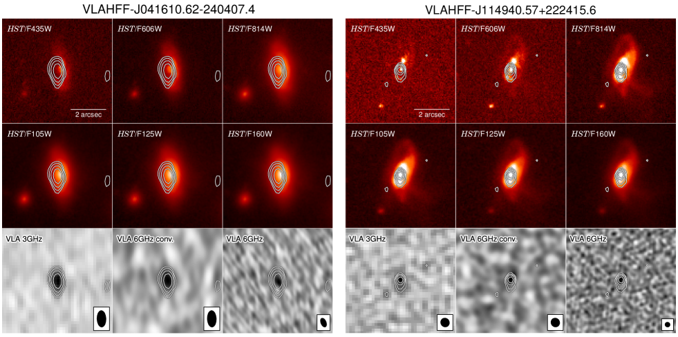
Figure 1: The multi-wavelength view of the morphology of galaxies in the HFF. Two examples are presented: VLAHFF-J041610.62-240407.4 at $z=0.41$ and VLAHFF-J114940.57+222415.6 at $z=0.76$. The two upper rows show stamps from the six HST bands used in this study, while the bottom row presents the stamps from the VLA map at 3 and 6 GHz (including the original and the convolved image to the resolution of the 3 GHz map). The size of the synthesized beam is shown at the bottom-right corner of the stamps. The contour levels start at $3\sigma\simeq 3\rm\mu Jy\,beam^{-1}$ and are spaced on a logarithmic scale. The stamps for all the galaxies in the sample are available at https://science.nrao.edu/science/surveys/vla-ff/data.

2.2 HST data

We use HST observations taken with the ACS and WFC3 instruments as part of the HFF program (Lotz et al., 2017, Koekemoer et al. submitted). We employ the images from the wide-band filters ACS/F435W, ACS/F606W, ACS/F814W, WFC3/F105W, WFC3/F125W, and WFC3/F160W. Combined, these images continuously cover the observed wavelength range of 0.35$-$1.7$\,\mu$m, i.e., the optical-to-near-IR regime (see Figure 1). For galaxies over the redshift range $1\lesssim z\lesssim 2$ we can simultaneously observe the rest-frame UV (0.15$-$0.3$\,\mu$m) and optical (0.45$-$0.8$\,\mu$m) continuum emission. For galaxies at $z\lesssim 1$, we can observe their rest-frame optical emission through the ACS HST filters, while the WFC3 HST filters trace the rest-frame UV emission of $z\gtrsim 2$ galaxies.

We employ the final mosaics (with 60 mas pixel scale) of MACS J0416-2403, MACS J0717+3745, and MACS J1149+2223 (cluster and parallel fields) produced by the HFF DeepSpace team (Shipley et al., 2018), which, combined, encompass a sky area of $\approx 68\,\rm arcmin^{2}$. These are stacked and drizzled images (version v1.0) from the HFF program (Lotz et al., 2017, Koekemoer et al. submitted.), in which major artifacts and cosmic rays were removed. We also download the segmentation maps and PSFs, required in this work, that have been produced and released to the public by the HFF DeepSpace team. The PSFs have been empirically derived by stacking non-saturated stars per each of the HFF fields and HST filters (Shipley et al., 2018). A 2D Gaussian fit to the PSFs indicates an average ${\rm FWHM}\approx 0\farcs 11$ and 0$\farcs$18 resolution for the ACS and WFC3 images.

2.3 The VLA Frontier Fields catalogs

Our galaxy sample is drawn from the VLA Frontier Fields catalog (Heywood et al. in press). This compilation contains information for 1966 and 257 compact radio sources detected at 3 GHz and 6 GHz, respectively, across the three HFF cluster and parallel fields explored here. A minimum signal-to-noise ratio ($S/N$) threshold of 5 was adopted to detect the radio sources with the PyBDSF code (Mohan & Rafferty, 2015). Flux density and FWHM estimates of radio sources (before and after deconvolution) are also reported in the catalog.

The VLA Frontier Fields catalog also reports spectroscopic/photometric redshifts and stellar masses of radio sources with a counterpart in the HFF-DeepSpace Photometric Catalogs (Shipley et al., 2018). 113 radio-selected galaxies with available redshift and stellar mass estimates are identified. The low fraction of 3 GHz-detected sources with a counterpart in the HFF-DeepSpace Catalogs is a result of the large sky coverage of the VLA 3 GHz radio maps, which is $\sim 14$ times that of the Hubble Frontier Fields themselves. Photometric redshifts were derived by Shipley et al. (2018) via spectral energy distribution (SED) fitting with the eazy code (Brammer et al., 2008). The photometric redshift used here corresponds to the peak of the redshift distribution. These photometric estimates are found to be in good agreement with available spectroscopic redshifts, as Shipley et al. (2018) finds an average dispersion of $\sigma=0.034$ and a gross failure rate of $\lesssim 10\%$. Using such redshift estimates, Heywood et al. ( in press) estimated the lensing magnification factors for these radio sources using all available lensing models from the Frontier Fields team (e.g., Jauzac et al., 2012, 2014; Johnson et al., 2014). The median magnification factor $(\mu)$, recorded in the VLA Frontier Fields catalog, is used throughout this paper to derive the intrinsic properties of our galaxy sample. Photometric redshifts, or spectroscopic estimates when available, were also used by Shipley et al. (2018) to derive stellar masses with the fast code (Kriek et al., 2009). To this end, the Bruzual & Charlot (2003) stellar population synthesis model library and the Calzetti et al. (2000) dust attenuation law was employed. A Chabrier (2003) IMF, solar metallicity, and exponentially declining star formation histories were adopted as well. These stellar mass estimates ($M_{\star}^{\rm FAST}$) are here corrected for lensing magnification as follows: $M_{\star}=M_{\star}^{\rm FAST}/\mu$, where $\mu$ is the median magnification factor reported by Heywood et al. ( in press).

3 Analysis

3.1 The sample

We select the 113 galaxies in the VLA Frontier Fields 3 GHz catalog with available redshift and stellar mass estimates from the HFF DeepSpace catalogs. 31 of these are also detected at 6 GHz. A total of 14 (7), 38 (15) and 32 (7) sources are identified in the MACS J0416, MACS J0717 and MACS J1149 cluster (parallel) fields, respectively. The smaller numbers of sources in the parallel fields is a result of the cluster overdensity, as well as the reduced radio sensitivity and negligible lensing magnification at the positions of the parallel fields.

3.1.1 Selecting field galaxies in the HFF

We remove cluster galaxies from the sample to account for the potential biases linked to the environmental dependence of galaxy evolution. This is done by selecting sources that are inside the projected cluster virial radius, and that have line-of-sight velocities falling within the velocity dispersion of galaxies in the clusters. In this case, the virial radius of these complexes ($\sim$2 Mpc/5′; e.g., Balestra et al., 2016) is larger than the extent of the HST mosaics of the HFF clusters ($\sim 2\arcmin$ radius). As a result, the selection of cluster galaxies only relies on their line-of-sight velocity ($v_{\rm gal}={\rm c}z_{\rm gal}$). Accordingly, we recognize cluster galaxies as those satisfying the condition $|z_{\rm gal}-z_{\rm cluster}|<3\sigma_{z}$, where $z_{\rm cluster}$ is the redshift of the HFF clusters, $\sigma_{z}$ the associated redshift dispersion, and $z_{\rm gal}$ the redshift of the galaxy of interest. The values of $z_{\rm cluster}$ $(\sigma_{z})$ are 0.3972 (0.0033), 0.5450 (0.0036), and 0.5422 (0.0048) for MACS J0416 (Balestra et al., 2016), MACS J0717 (Richard et al., 2014), and MACS J1149 (Grillo et al., 2016), respectively. This analysis identifies 15 cluster galaxies out of the initial 113 galaxies, leading to a sample of 98 field galaxies with available redshift and stellar mass estimates. Although the focus of this study is the nature of field galaxies, in Table 2, we also report the radio/UV/optical sizes of those 15 cluster galaxies.

3.1.2 Magnification factor, redshift, and stellar mass distribution

The median magnification factor of the 98 field galaxies in our sample is $\mu=1.1^{+0.6}_{-0.1}$, where the upper/lower limit correspond to the 84th/16th percentile of the distribution. Only a small fraction ($\approx 13\%$) are moderately lensed with magnification factors between 2 and 6 (Figure 2). Because morphological parameters of lensed galaxies with $\mu<30$ can be derived without introducing strong biases (Florian et al., 2016), we also include moderately lensed galaxies in our sample. We verified that none of the results presented here significantly change if sources with $\mu\geq 2$ are excluded from the analysis.

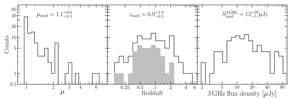
Figure 2: Distribution of the magnification factor (left panel), redshift (middle panel), and 3 GHz flux density (right panel) of 98 radio-selected, field galaxies in the HFF fields, for which information about their stellar masses and UV/optical photometry are available in the HFF DeepSpace catalogs. The median of the distributions is shown at the top, the lower/upper limits correspond to the 16th/84th percentile of the distribution. The grey filled histogram shows the distribution of 40 galaxies with available spectroscopic redshift, whose median is $0.7^{+0.4}_{-0.3}$. The 3 GHz flux density has been corrected by lensing magnification.

The redshift distribution (Figure 2) of the final sample of 98 galaxies has a median of $z=0.9$ and 16th/84th percentiles of $z=0.4/1.9$, respectively. In our sample, 41% of galaxies have spectroscopic redshifts. The median and 16th/84th percentiles of the spectroscopic redshift distribution are $0.7^{+0.4}_{-0.3}$. The distribution of the stellar mass of galaxies (Figure 3) in the sample has a median of $\log(M_{\star}/\rm M_{\odot})=10.4^{+0.4}_{-0.6}$. The scarcely sampled mass regime below $\log(M_{\star}/\rm M_{\odot})<10$ is a result of our radio detection limits that select massive, bright systems. We thus expect that a mass-complete (representative) sample of radio-selected sources can be assembled by considering galaxies with $\log(M_{\star}/\rm M_{\odot})\gtrsim 10$.

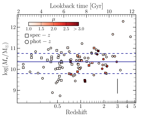
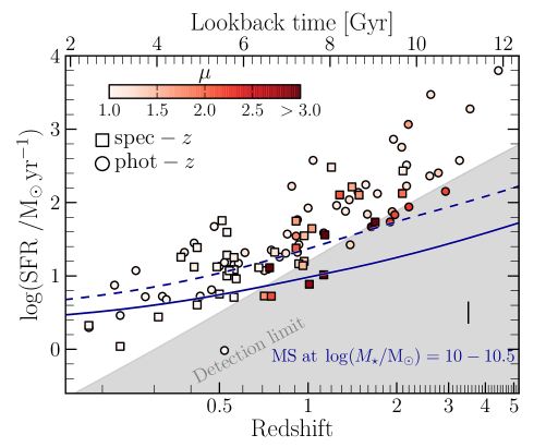
Figure 3: Lensing-corrected stellar mass (left panel) and SFR (right panel) as function of the redshift of 98 galaxies in our sample, of which 40 have available spectroscopic redshift (squares). For the remaining 58 galaxies, we use photometric redshift estimates (circles). The data points are color-coded according to the galaxies magnification factor. The horizontal solid and dashed lines in the left panel show the 50th and 16th/84th percentiles of the stellar mass distribution, correspondingly. Thanks to the $\mu\rm Jy$-level sensitivity of the HFF-VLA radio maps and the lensed-nature of our galaxy sample, we can detect typical, main sequence SFGs with $\log(M_{\star}/\rm M_{\odot})=10.5$ out to $z\simeq 3$. The grey shaded region on the right panel shows our detection limit, which is given by the SFR of a galaxy detected at the $5\sigma\;(\simeq 4.5\mu\rm Jy\,beam^{-1})$ significance level at a given redshift. The solid and dashed line indicate the redshift evolution of the main sequence (from Schreiber et al., 2015) for galaxies with stellar mass of $\log(M_{\star}/\rm M_{\odot})=10$ and $10.5$, respectively. The moderate magnification factor ($\mu>2$) of a minor fraction of galaxies allows us to probe lower SFRs than that SFR limit imposed by the radio maps noise.

3.1.3 AGN fraction

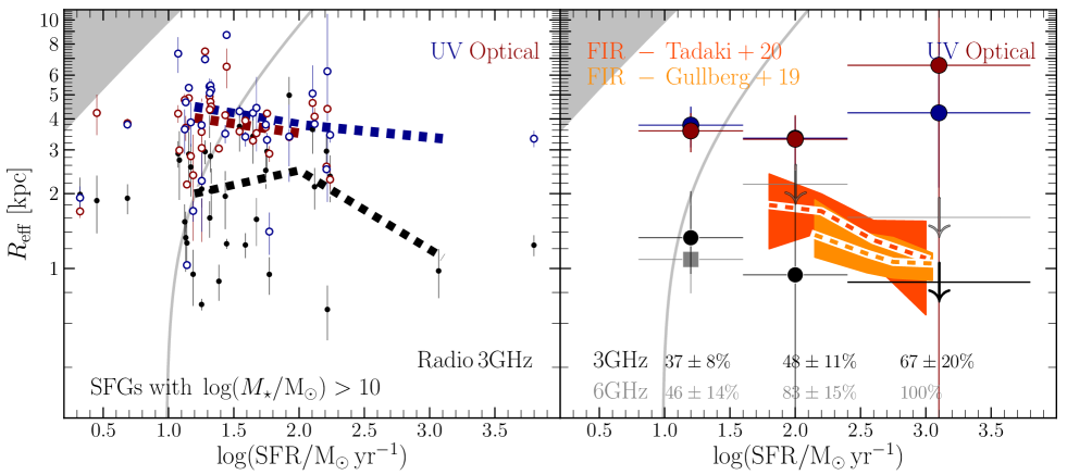
Figure 14: Left panel– The radio/UV/optical effective radius of $\log(M_{\star}/\rm M_{\odot})>10$ SFGs that are reliably resolved at 3 GHz as a function of their SFR. The dashed lines show the median effective radius per SFR bin ($1-1.5$ dex width). Right panel– The median radio/UV/optical effective radius of all galaxies in the sample (i.e., sources that are reliably and unreliably resolved at 3 GHz) per SFR bin. Contrary to the results presented in Figure 10, here we exclude the radio sources that have an X-ray counterpart, which are likely to host an AGN. A complete description of this figure can be found in the caption of Figure 10.

To determine the AGN fraction in our final sample, we rely on results from semi-empirical simulations (Wilman et al., 2008) and observations of the faint radio source population (e.g., Bonzini et al., 2013; Smolčić et al., 2017b). These studies indicate that at radio flux densities below $\sim 100\,\rm\mu Jy$ at $1.4-3$ GHz, the radio population is dominated by SFGs. Galaxies in our sample have a median 3 GHz flux density of just $13^{+20}_{-5}\,\rm\mu Jy$ (Figure 2), where the upper/lower values correspond to the 84th/16th percentile of the flux density distribution. Based on the typical radio flux densities and predictions from Smolčić et al. (2017b, see their Figure 14), we expect that $\approx 75\%$ of galaxies in our sample selected at 3 GHz are “pure” SFGs, while the remaining fraction (i.e., 25%) are galaxies with some potential contribution from AGN radio luminosity. In an attempt to identify those AGN candidates, we use the Chandra Source Catalog Release 2.0 (Evans et al., 2010) and the X-ray catalog of MACSJ0717 from van Weeren et al. (2016) to find X-ray counterparts of radio sources in our sample. We find 12 positional coincidences within a 1″search radius (see Table 2). All of them have an X-ray luminosity ([$0.5-10$] keV) of $L_{\rm X}\approx 10^{42.5-44.8}\,\rm erg\,s^{-1}$ that is higher than the typical limit of $L_{\rm X}=10^{42}\,\rm erg\,s^{-1}$ to select X-ray AGN (e.g., Szokoly et al., 2004). These X-ray detected galaxies represent 11% of the total sample, thereby, the radio emission of galaxies in our sample is dominated by star formation processes. We further discuss the implications of AGN-dominated sources in the relations presented in §4.

3.1.4 Radio spectral index

Out of our sample of 98 field galaxies simultaneously detected in the 3 GHz radio map and HST images, 31 of them are also detected in the 6 GHz image. Spectral indices measured from the 3 and 6 GHz flux densities, i.e., $\alpha_{\rm 6\,GHz/3\,GHz}$, are available for these sources in the VLA HFF catalogs (Heywood et al.  in press). Note that the low fraction of sources detected at 6 GHz is mainly due to the fainter radio flux density of SFGs at 6 GHz, as well as the smaller area of the 6 GHz maps that do not fully cover the HFF parallel fields. We derive a median $\alpha_{\rm 6\,GHz/3\,GHz}$ of $0.68^{+0.28}_{-0.46}$. This value is consistent with the typical radio spectral index of radio-selected SFGs of $\alpha\approx 0.7$ (e.g., Condon, 1992; Smolčić et al., 2017a).

3.2 Deriving star formation rates from radio/UV emission

To derive total SFRs from the radio (dust-unobscured) and UV (dust-obscured) emission of galaxies, we employ the SFR calibrations from Murphy et al. (2011, 2012b, 2017) who adopt a Kroupa IMF. We normalize such SFR calibrations to the Chabrier IMF, to be consistent with the IMF employed by (Shipley et al., 2018) to derive the stellar masses used here. Note that the Chabrier IMF leads to SFR and stellar mass estimates that are only $\approx 6$% lower than those values inferred from a Kroupa IMF.

Using the locally measured IR-radio correlation from Bell (2003, i.e., $q_{\rm IR}=2.64$), the unobscured SFR of a galaxy can be estimated from its 1.4 GHz spectral luminosity, $L_{\rm 1.4\,GHz}$, as (Murphy et al., 2017):

$$\left(\frac{\rm{SFR_{3\,GHz}}}{\rm M_{\odot}\,yr^{-1}}\right)=4.87\times 10^{-29}\;\left(\frac{L_{\rm 1.4\,GHz}}{\rm erg\,s^{-1}\,Hz^{-1}}\right).$$ (1)

$L_{\rm 1.4\,GHz}$ is given by

$$L_{\rm 1.4\,GHz}=\frac{4\pi D_{\rm L}(z)^{2}}{(1+z)^{1-\alpha}}\left(\frac{1.4}{3}\right)^{-\alpha}S_{\rm 3\,GHz},$$ (2)

where $S_{\rm 3\,GHz}$ is the 3 GHz flux density in $\rm erg\,s^{-1}\,cm^{-2}\,Hz^{-1}$, $D_{\rm L}$ is the luminosity distance in cm, and $\alpha$ is the spectral index of the power-law radio emission given by $S_{\nu}\propto\nu^{-\alpha}$. As mentioned in §3.1.4, an estimate of $\alpha$ is available for 31 sources with 6 GHz counterpart. We estimate the $\rm SFR_{3\,GHz}$ of the remaining sources by adopting the typical spectral index of 3 GHz radio-selected SFGs of $\alpha=0.7$ (e.g., Smolčić et al., 2017a). This simplification introduces further uncertainties to our $\rm SFR_{3\,GHz}$ estimates, which we quantify by using the 31 galaxies with available 6 GHz counterpart to compare their $\rm SFR_{3\,GHz}$ derived from $\alpha_{\rm 6\,GHz/3\,GHz}$ and $\rm\alpha=0.7$. We find that both estimates are well-correlated, with a dispersion of only $30\%$. We hence include an additional systematic error of 30% to our single-band $\rm SFR_{3\,GHz}(\alpha=0.7)$ estimates.

The unobscured SFR of galaxies is estimated using the rest-frame far-UV (FUV) luminosity at 1600Å, $L_{\rm FUV}$, which is sensitive to young (unobscured) stellar populations (up to ages around 8 Myr; e.g., Cerviño et al., 2016). $L_{\rm FUV}$ is estimated from the FUV magnitude obtained with eazy and reported in the HFF DeepSpace catalogs (Shipley et al., 2018). Then, the FUV-based SFR is estimated from the (extinction-corrected) FUV luminosity as (Murphy et al., 2012b):

$$\left(\frac{\rm{SFR_{FUV}}}{\rm M_{\odot}\,yr^{-1}}\right)=4.17\times 10^{-44}\;\left(\frac{L_{\rm FUV}}{\rm erg\,s^{-1}}\right).$$ (3)

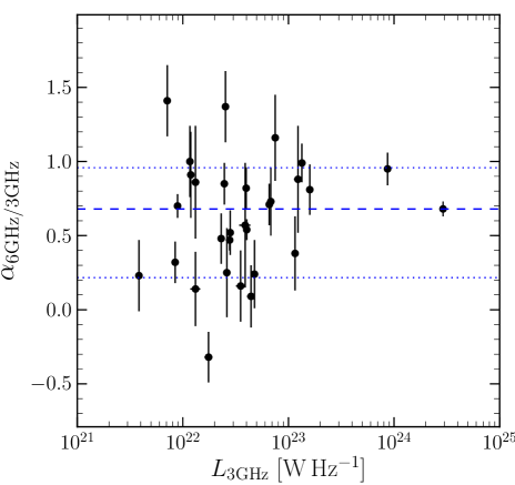
Figure 4: Radio spectral index as a function of 3 GHz radio luminosity of 31 galaxies in our sample detected at both 3  and 6 GHz radio maps. The horizontal dotted line shows the median spectral index of 0.68, while the dashed lines show the 16th and 84th percentiles. The median spectral index of these galaxies is consistent with the typical value of radio-selected SFGs of 0.7.

In Equation 3, $\rm SFR_{FUV}$ is computed using the FUV as observed (i.e, it has not been corrected for internal dust extinction) to only account for the unobscured component. Finally, the total, lensing-corrected SFR of galaxies can be estimated as

$$\rm{SFR=(SFR_{3\,GHz}+SFR_{FUV})/\mu},$$ (4)

where $\rm SFR_{3\,GHz}$ accounts for the population of young stars that is totally obscured by dust, and $\rm SFR_{FUV}$ reflects the contribution of unobscured young stars. Comparing the $\rm SFR_{3\,GHz}$ with $\rm SFR_{FUV}$ (see Appendix A), we find that radio-based SFRs account for $\gtrsim 95\%$ of the total SFR of massive SFGs with $\log(M_{\star}/\rm M_{\odot})>10$. Using FUV emission that is not corrected for dust attenuation can thus lead to SFRs that are underestimated, on average, by one order of magnitude. Likewise, we find that the optical-infrared (OIR) SFRs from SED fitting (reported in the HFF-DeepSpace catalogs) are unreliable, showing no correlation and one order of magnitude scatter with the radio-based SFRs (see Appendix A). These results strengthen the approach of adopting $\rm SFR_{3\,GHz}$, combined with $\rm SFR_{FUV}$, to better trace the total energetic budget arising from massive star formation in galaxies.

In Figure 3, we present the total, lensing-corrected SFRs and stellar mass as a function of the redshift of 98 field galaxies in our sample. The noise of $0.9\,\rm\mu Jy\,beam^{-1}$ of the 3 GHz VLA HFF maps enables detection of “typical” SFGs on the main sequence (e.g., Schreiber et al., 2015) out to $z\approx 3$ with $\log(M_{\star}/\rm M_{\odot})\approx 10.5$, which is the median stellar mass of galaxies in our sample. Figure 3 also illustrates the benefits of selecting galaxies towards the HFF. By detecting intrinsically faint sources that without gravitational lensing would not have been detected with a $\rm 0.9\,\mu Jy\,beam^{-1}$ sensitivity, we are able to better sample the population of massive SFGs with $\log(M_{\star}/\rm M_{\odot})>10$ out to $z\approx 3$.

3.3 Estimating the radio size of galaxies

Heywood et al. ( in press) have reported the deconvolved FWHM ($\theta_{\rm M}$, and its associated uncertainty, $\sigma_{\theta_{\rm M}}$) of galaxies in the VLA Frontier Fields, including results from the 3 GHz and 6 GHz imaging. Sources have been considered reliably resolved if they satisfy the condition $\phi_{\rm M}-\theta_{\rm 1/2}\geq 2\sigma_{\phi_{\rm M}}$; where $\phi_{\rm M}$ and $\sigma_{\phi_{\rm M}}$ are the major axis FWHM of the source before deconvolution and its associated error (provided by PyBDSF), and $\theta_{\rm 1/2}$ the FWHM of the beam projected along with the source PA (see Appendix A  of Heywood et al.  in press). For sources that are not confidently resolved, here we assign $\theta_{\rm M}+\sigma_{\theta_{\rm M}}$ as an upper limit of their deconvolved FWHM.

To compare the radio size of galaxies at 3 GHz and 6 GHz, we convolve the 6 GHz images to match the beam size and shape of the 3 GHz images (Figure 1). This procedure is critical to minimize systematic effects when comparing the radio size of compact sources at different spatial resolutions. For example, the total flux density and, hence, the size of moderately resolved sources can differ between radio maps with different spatial resolutions (Murphy et al., 2017; Bondi et al., 2018). We then use PyBDSF to perform the source extraction and size measurement with the same parameters used by Heywood et al. ( in press): a $S/N$ threshold of 5 to detect peaks of emission and a secondary $S/N$ threshold of 3 to identify the pixels (islands of emission) associated to those peaks. The errors and upper limits to the radio size from these convolved images at 6 GHz are derived as in Heywood et al. ( in press). This new catalog is combined with information from the 3 GHz imaging from Heywood et al. ( in press) to get a matched-resolution ($\approx 0\farcs 7$) catalog containing the radio size (and error) estimates of galaxies in the sample at 3 GHz and 6 GHz. Around 50% of the 3 and 6 GHz radio sources in our sample are reliably resolved: 53 out of the 98 at 3 GHz, and 12 out of 31 at 6 GHz.

Finally, since our sources are only marginally resolved (i.e., $R_{\rm eff-rad}\lesssim\theta_{\rm 1/2}$, see an example in Figure 1), the effective radii of the radio sizes is well approximated by $R_{\rm eff-rad}\approx\theta_{\rm M}/2.430$ (Murphy et al., 2017), where $\theta_{\rm M}$ is the deconvolved FWHM provided by PyBDSF. In applying this approximation we assume that most galaxies in the sample are exponential disks, which is consistent with the Sérsic index of $n\approx 1$ reported for typical SFGs (using stellar emission; Nelson et al., 2016) and even highly-active SFGs at $z\gtrsim 2$ (using dust continuum emission; Hodge et al., 2016, 2019; Gullberg et al., 2019; Tadaki et al., 2020). This approximation might deviate from the true effective radius of galaxies that have cuspier light profiles, including a fraction of compact quiescent and starburst galaxies (e.g., Wuyts et al., 2011). However, even with an angular resolution that is three times better than ours, Elbaz et al. (2018) finds no significant changes in the effective radius of $z\sim 2$ compact galaxies (from dust continuum emission) if Sérsic indices higher than one are used. Finally, the effective radius is corrected for lensing magnification as follows: $R_{\rm eff-rad}^{\rm cor}=R_{\rm eff-rad}/\sqrt{\mu}$. For simplicity, in the following, we refer to this lensing-corrected effective radius as $R_{\rm eff}$.

3.4 Estimating the UV/optical size of galaxies

We use the Python package statmorph (Rodriguez-Gomez et al., 2018) to derive the UV/optical effective radius of galaxies in the sample. This radius is estimated for each of the six HST bands used in this work (Figure 1), but only for those galaxies flagged with good photometric data (flag=0) in the HFF DeepSpace catalog (Shipley et al., 2018). Most galaxies ($>95\%$) profit from robust photometric imaging in the HST/ACS bands, whereas around $60\%$ of them are also covered by the HST/WFC3 imaging.

To implement statmorph, we first create $15\arcsec\times 15\arcsec$  width cutouts per each of the six HST photometric bands. Then, the background is estimated (and subtracted from the original image) through sigma-clipped statistics with the photutils Python library. We independently create segmentation maps for the Brightest Cluster Galaxies (BCGs) as these are not available in the HFF DeepSpace project. This is done with the photutils.SegmentationImage and photutils.deblend-sources libraries that enable us to deblend the emission of the BCGs and neighboring sources.

The effective (half-light) radius is estimated by using elliptical apertures centered at the asymmetry center of the galaxy emission. The outer radius containing the total flux of the galaxy, $R_{\rm max}$, is defined in statmorph as the distance between the asymmetric center of the galaxy emission and the most distant pixel within the detection mask. This mask is derived by smoothing the galaxy image with a $3\times 3$ boxcar kernel and considering the contiguous group of pixels that are $1\sigma$ above the mode (Rodriguez-Gomez et al., 2018). We neglect the size estimates that are flagged by statmorph as not physically meaningful quantities. This type of results represents less than 10% of total outputs. Finally, to consider the effect of the PSF on our $R_{\rm eff}$ estimates, we apply the relation $R_{\rm eff}^{\rm intrinsic}=(R_{\rm eff}^{2}-R_{\rm PSF}^{2})^{1/2}$; where $R_{\rm PSF}$ has been derived following the same non-parametric analysis on the PSF images, and $R_{\rm eff}^{\rm intrinsic}$ is the PSF-corrected effective radius. The lensing magnification is also corrected by evaluating: $R_{\rm eff}^{\rm cor}=R_{\rm eff}^{\rm intrinsic}/\sqrt{\mu}$. In the following, we simply refer to the PSF- and lensing-corrected effective radius as $R_{\rm eff}$.

The code statmorph also fits 2D Sérsic models to the galaxy emission from which the effective radius, $R_{\rm eff}^{\rm Sersic}$, is also derived. We verified that $R_{\rm eff}^{\rm Sersic}$ and the non-parametric $R_{\rm eff}$ estimates are consistent. The $R_{\rm eff}-R_{\rm eff}^{\rm Sersic}$ relation shows a dispersion of $\sim 0.2$ dex. In the case of extended galaxies, however, $R^{\rm Sersic}_{\rm eff}$ tends to be higher than $R_{\rm eff}$ as a 2D Sérsic model fails to reproduce the clumpy structure of extended, well-resolved galaxies in our sample.

3.4.1 Wavelength dependence of the galaxy size in the UV-to-optical regime

To investigate the UV/optical size evolution of galaxies across cosmic time, we need to consider the effects of the morphological $k$-correction (e.g., Conselice, 2014). As the redshift increases, the ACS and WFC3 filters probe different regimes of the galaxy spectrum and hence distinct stellar populations. Without correcting for this effect, the inferred size evolution of galaxies might simply reflect the dependence of the galaxy size on the wavelength. To explore such a correlation, we present in Figure 5 the effective radius measured from the ACS and WFC3 imaging as a function of the rest-frame wavelength. For each galaxy, the effective radius derived from the different HST filters, $R_{\rm eff}(\rm band)$, has been normalized to the median value $\tilde{R}_{\rm eff}$. In all but the highest redshift bin, we find that the size of galaxies varies, on average, less than 10% across all the HST filters used in this study. This is consistent with the smooth evolution of the UV-to-optical size of galaxies previously reported in the literature (e.g., van der Wel et al., 2014; Vika et al., 2015; Ribeiro et al., 2016). At $z>2$, we observe a steep increment of the galaxy size at longer wavelengths; however, this trend is driven by a small number of data points and hence it is associated with a high degree of uncertainty. Finally, we verify that the wavelength dependence of the galaxy size in the UV-to-optical regime (Figure 5) does not significantly change if galaxies with different mass and SFR are considered.

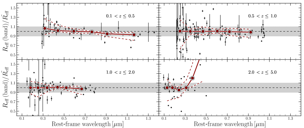
Figure 5: The effective radius of galaxies at a fixed rest-frame wavelength, $R_{\rm eff}({\rm band})$, measured from the six HST bands. The values in the ordinate have been normalized to the median effective radius ($\tilde{R}_{\rm eff}$) from the six HST bands. Four different redshift bins are presented. The grey circles show the $R_{\rm eff}({\rm band})/\tilde{R}_{\rm eff}$ ratio for all the galaxies in the sample and for all the HST bands used here. The magenta circles show the median $R_{\rm eff}({\rm band})/\tilde{R}_{\rm eff}$ ratio per HST band, while the dashed blue lines show their associated dispersion (16th and 84th percentiles). The grey shaded region illustrates the $\pm 10\%$ variance with respect to the median effective radius from the six HST bands. The dashed horizontal line is set at $R_{\rm eff}({\rm band})/\tilde{R}_{\rm eff}=1$. This plot demonstrates that the effective radius of most galaxies in the sample remains constant across the UV-to-optical regime.

Given the smooth variations of galaxy size throughout UV-to-optical wavelengths, a single measurement over $0.1-0.4\,\mu$m and $0.4-1.0\,\mu$m can provide an estimate for the size of galaxies in the rest-frame UV and optical regime, respectively. Therefore, we group all the available size measurements falling within the UV ($0.1-0.4\,\mu$m) and optical ($0.4-1.0\,\mu$m) rest-frame wavelength ranges, and report the corresponding median value as the UV and optical size of galaxies.

3.5 Strengths and limitations of our size measurements

Comprehensive simulations that investigate the biases and uncertainties in measuring the size of galaxies from UV/optical imaging have been performed (Meert et al., 2013; Mosleh et al., 2013; Davari et al., 2014). The consensus is that either parametric (e.g., fitting Sérsic profiles) or non-parametric methods can retrieve the size of galaxies with $S/N\gtrsim 10$ without introducing strong systematic errors (up to 20%). Past studies also suggest that the cosmological surface brightness dimming does not significantly affect the UV/optical size measurement of galaxies out to $z\sim 4$ (Paulino-Afonso et al., 2016; Ribeiro et al., 2016). Particularly, using simulations of HST observations, Davari et al. (2014) find that there are no significant biases in the effective radius inferred from the cumulative radial flux distribution of galaxies – as those derived here. For galaxies with $R_{\rm eff}\gtrsim 0\farcs 1$, as in our sample, the UV/optical sizes can be measured without introducing strong biases and with $\lesssim 5\%$ uncertainties (Davari et al., 2014, see their Figure 3).

However, because high-redshift galaxies exhibit faint radio emission that is centrally concentrated (e.g., Murphy et al., 2017; Bondi et al., 2018; Jiménez-Andrade et al., 2019), measuring the radio size is challenging even with the deep, high-resolution (sub-arcsec) radio observations delivered by the HFF VLA survey. Contrary to the UV/optical emission that is spatially resolved across multiple resolution elements, our radio sources are slightly resolved, which could lead to systematic uncertainties in our size measurements. To verify this, we infer $R_{\rm eff}$ from the $S_{\rm peak}/S_{\rm int}$ ratio for a circular exponential disk observed with a circular Gaussian beam. This ratio is given by (see Appendix C of Murphy et al., 2017):

$$\frac{S_{\rm peak}}{S_{\rm int}}=2z^{2}\left[1-\sqrt{\pi}z\exp(z^{2}){\rm erfc}(z)\right],$$ (5)

where $z\approx 0.50398\left(\theta_{1/2}/R_{\rm eff}\right)$, with $\theta_{1/2}$ the FWHM of a circular beam. While Equation 5 is valid for a circular (face-on) exponential disk, the $S_{\rm peak}/S_{\rm int}$ ratio of an elliptical (inclined) exponential disk can be estimated as

$$\frac{S_{\rm peak}}{S_{\rm int}}\approx\left[\left(\frac{S_{\rm peak}}{S_{\rm int}}\right)_{\rm M}\left(\frac{S_{\rm peak}}{S_{\rm int}}\right)_{\rm m}\right]^{1/2},$$ (6)

where $(S_{\rm peak}/S_{\rm int})_{\rm M}$ and $(S_{\rm peak}/S_{\rm int})_{\rm m}$ are the respective $S_{\rm peak}/S_{\rm int}$ ratios along the major (M) and minor (m) axes of an elliptical disk.

In Figure 6, we present the observed and expected $S_{\rm peak}/S_{\rm int}-R_{\rm eff}$ relation of sources in the MACS J1149, MACS J0717, and MACS J0416 fields. We find that the effective radius of reliably resolved sources lies between the expected value for an edge-on and face-on disk. Such an agreement, between the observed and expected $S_{\rm peak}/S_{\rm int}-R_{\rm eff}$ relation, strengthens the reliability of our size measurements via 2D Gaussian fitting with PyBDSF.

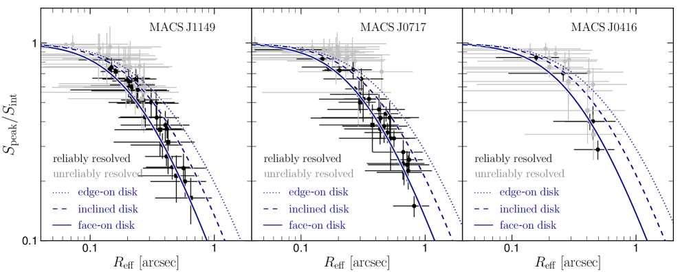
Figure 6: The ratio of peak-to-integrated flux densities, $S_{\rm peak}/S_{\rm int}$, of sources in our sample as a function of the deconvolved disk effective radius, $R_{\rm eff}$, in units of arcsec. We present the $S_{\rm peak}/S_{\rm int}-R_{\rm eff}$ relation for SFGs in the MACS J1149, MACS J0717, and MACS J0416 fields separately, to account for the different spatial resolution of their respective VLA radio image. The black circles (squares) show the reliably resolved sources at 3 GHz (6 GHz), while the grey symbols represent the unreliably resolved sources. The expected $S_{\rm peak}/S_{\rm int}-R_{\rm eff}$ relation for a a circular (face-on) exponential disk is shown by the solid blue line (Equation 5). The dashed blue lines shows the $S_{\rm peak}/S_{\rm int}-R_{\rm eff}$ relation for an inclined disk [$\cos(i)=0.5$, with $i$ the inclination angle], whereas the dotted blue line corresponds to a nearly face-on disk [$\cos(i)=0.25$]. This demonstrates that the size of reliably resolved sources meets expectations from their $S_{\rm peak}/S_{\rm int}$ ratio.

3.6 Maximum recovered radio size

We use Equations 5 and 6 to infer the maximum detectable angular size as a function of flux density of sources in our sample. This allows us to derive the maximum radio size of galaxies that can be detected at a given redshift, stellar mass, and SFR. To this end, we solve for $R_{\rm eff}$ in Equation 5 using the Newton-Raphson method with the scipy.optimize library in Python. We then evaluate $R_{\rm eff}(S_{\rm int})$ using the respective FWHM of the major and minor axis of the beam and rms noise level from the three different HFF radio images (see Figure 7). The selection function imposed by the resolution and sensitivity of the MACSJ0416, MACSJ0717, and MACSJ1149 radio images is consistent: galaxies with flux densities below 10$\mu Jy$, close to the detection limit, are preferentially detected when they are compact. Also, due to their faint nature, such compact sources can not be reliably resolved. We discuss the effects of this selection function in the results presented in §4.2 and 4.3.

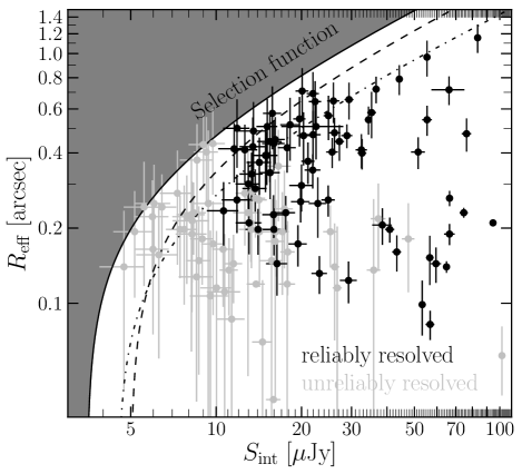
Figure 7: Maximum detectable angular size as a function of total flux density of sources in the HFF radio images: MACSJ0416 (dashed line), MACSJ0717 (solid line), MACSJ1149 (dash-dotted line). Reliably resolved sources are shown as black circles, while those unreliably resolved are presented in grey. Close to the detection limit, our selection function bias the sample toward compact sources that can not be reliably resolved.

4 Results and Discussion

In this Section, we compare the radio size of galaxies measured at 3 and 6 GHz (§4.1) and investigate the dependence of the galaxy size on stellar mass (§4.2), star formation activity (§4.3), and redshift (§4.4). The redshift, SFR, stellar mass, and multi-wavelength size estimates of all the galaxies in our sample are presented in Table 2.

4.1 Comparing the radio size of galaxies at 3 GHz and 6 GHz

In Figure 8, we compare the radio sizes of galaxies at 3 GHz and 6 GHz from our VLA Frontier Fields images. Out of the initial sample of 98 radio-selected galaxies, 31 of them are detected in the matched-resolution radio images at 3 GHz and 6 GHz. Among these common sources, 25 are reliably resolved at 3 GHz, and only 12 at 6 GHz. As a result, our data set is dominated by upper limits to the size of galaxies that are not reliably resolved at 6 GHz. To derive median properties of this censored data set, we use survival analysis via the Kaplan & Meier (KM; 1958) estimator with the Python package lifelines. This statistical technique employs the censored sample, where upper limits are present, to provide a maximum-likelihood-type reconstruction of the true distribution function (Feigelson & Nelson, 1985).

We derive a median 3 GHz size of $R_{\rm eff}=1.3\pm 0.3\rm\,kpc$ for all the 98 galaxies in our sample, of which 53 are reliably resolved. For the 31 sources with available 3 and 6 GHz counterparts, we find a median $R_{\rm eff}$ of $1.3\pm 0.3\rm\,kpc$ at 3 GHz and $1.1^{+0.7}_{-0.3}\rm\,kpc$ at 6 GHz, where the upper/lower limits correspond to the 95% confidence interval for the median. Using Monte Carlo error propagation, we find that that the 3 GHz size is a factor $1.1\pm 0.1$ larger than the 6 GHz size of galaxies in the sample.

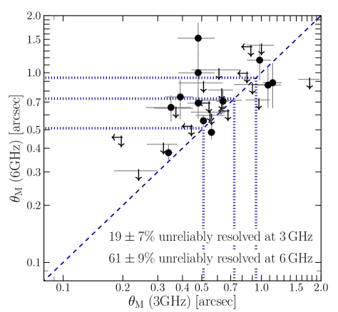
Figure 8: Deconvolved FWHM ($\theta_{\rm M}$) of the radio continuum emission of galaxies in 31 galaxies at 6 GHz as a function of the one measured at 3 GHz. The deconvolved FWHM at 6 GHz has been measured from the map that has been convolved to map the resolution of the 3 GHz map. The black circles show the galaxies for which both their sizes at 3 and 6 GHz are reliable resolved. The horizontal/vertical arrows are upper limits to the deconvolved FWHM at 3 GHz/6 GHz of sources that are not reliably resolved. The dashed diagonal line represents the one-to-one relation. The dotted vertical/horizontal lines correspond to the synthesized beam of the three VLA Frontier Fields images from which the 3 and 6 GHz size measurements are obtained. Even with a $\sim 0\farcs 7$ resolution, 19% (61%) of sources in our sample are not reliably resolved at 3 GHz (6 GHz). The larger fraction of sources unreliably resolved at 6 GHz hints toward the more compact radio size of galaxies at higher frequencies.

The radio continuum size of galaxies at 3 GHz has been previously explored. In the COSMOS field, Bondi et al. (2018) & Jiménez-Andrade et al. (2018) report a median effective radius of $1.5\pm 0.2$ kpc for massive SFGs $[\log(M_{\star}/M_{\odot})\lesssim 10.5]$ over $0.3\lesssim z\lesssim 3$; while Miettinen et al. (2017) finds a median effective radius of $1.9\pm 0.2$ kpc for 152 sub-millimeter selected galaxies over $1<z<6$ with a median redshift of $z=2.23\pm 0.13$. Similarly, Cotton et al. (2018) report a median 3 GHz effective radius of $1.0\pm 0.3\,$kpc for $z\approx 1$ SFGs in the Lockman-Hole. These values are in agreement, within the uncertainties, with the median effective radius of galaxies in our sample of $R_{\rm eff}=1.3\pm 0.3\rm\,kpc$. We attribute the scatter of these median $R_{\rm eff}$ values to the distinct selection criteria and different properties of the radio images. First, our sample might be “contaminated” by AGN (see §3.1) that could lead to more compact radio sizes (Bondi et al., 2018). This effect could account for the $\approx 15\%$ lower effective radius of galaxies in our sample with those from “pure” SFGs reported by Bondi et al. (2018) & Jiménez-Andrade et al. (2018). Second, the maximum detectable angular size of radio sources depends on both the resolution and sensitivity of radio maps (e.g., Bondi et al., 2008). Deeper, high-resolution radio surveys are more sensitive to compact radio sources. We thus expect that the median radio size of galaxies reported in the literature is influenced by the different depth and resolution of the radio maps.

There also exists information on the radio continuum size of galaxies at lower/higher frequencies. While our radio sizes at 3 and 6 GHz are two times larger than those at 10 GHz from $z\approx 1.2$ SFGs (Murphy et al., 2017), our 3 and 6 GHz sizes are two-to-three times smaller than those at 1.4 GHz from $0.2\lesssim z\lesssim 2$ SFGs (Muxlow et al., 2005, 2020; Lindroos et al., 2018). Such trends remain even if we compare the radio size of SFGs in our sample spanning over a similar redshift (and stellar mass) range than those studied by Murphy et al. (2017); Muxlow et al. (2005, 2020); Lindroos et al. (2018). These findings meet expectations from the frequency-dependent cosmic ray diffusion (but see Guidetti et al., 2017, who report large radio size of galaxies at 5.5 GHz). Lower-energy electrons emitting at lower frequencies can diffuse further into the ISM of galaxies as these have longer radiative lifetimes (Murphy, 2009; Thomson et al., 2019). As a result, the radio size of galaxies tends to decrease with increasing frequency. We further discuss the implications of frequency-dependent cosmic ray diffusion into the observed redshift-radio size relation in §4.4.

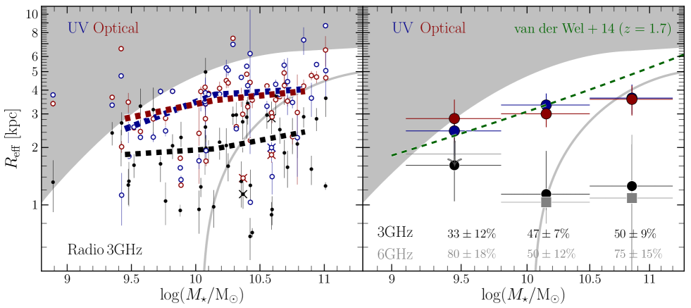
Figure 9: Left panel– The radio/UV/optical effective radius of galaxies that are reliably resolved at 3 GHz as a function of their stellar mass. The dashed lines show the median effective radius per stellar mass bin (0.75 dex width). The cross symbols denote the radio sources with a reported X-ray counterpart. Right panel– The median radio/UV/optical effective radius of all galaxies in the sample (i.e., sources that are reliably and unreliably resolved at 3 GHz) per stellar mass bin. To account for the upper limits to the radio sizes of unreliably resolved galaxies, we derive the median effective radius per stellar mass bin (and its associated uncertainty) via the KM estimator (Kaplan & Meier, 1958). The down arrows indicate the upper limit to the median size of galaxies per bin. The length of the error bars indicates the error of the median and the stellar mass bin, respectively. The grey curve shows the maximum $R_{\rm eff}$ that can be observed for a typical (main sequence) galaxy at $z=0.9$, which is the median redshift of our galaxy sample. The grey region illustrates the parameter space that can not be probed with our radio data set. The values at the bottom indicate the fraction of unreliably resolved galaxies at 3 and 6 GHz, respectively. In both panels, the UV/optical size of galaxies tend to increase with stellar mass, resembling –to some extent– the shallow slope of the stellar-mass relation of SFGs (e.g., van der Wel et al., 2014). There is no evident dependence between the radio size and stellar mass of SFGs in our sample.

4.2 Size vs stellar mass

To address the dependence of stellar mass on galaxy size, we distribute our galaxy sample into three mass bins: $9.1<\log(M_{\star}/\rm M_{\odot})\leq 9.8$, $9.8<\log(\rm M_{\star}/M_{\odot})\leq 10.5$, and $10.5<\log(M_{\star}/\rm M_{\odot})\leq 11.2$. We present the size – stellar mass relation for galaxies that are reliably resolved at 3 GHz (left panel of Figure 9) and all galaxies in the sample (i.e., reliably and unreliably resolved; right panel of Figure 9).

Using reliably resolved sources in the analysis, we find that the median radio size of SFGs mildly increases with stellar mass. Yet, this trend vanishes after considering unreliably resolved sources via survival analysis, indicating that there is no clear dependence between the radio size and stellar mass of SFGs (see Table 1). No robust constraints on the size – stellar mass relation can be inferred from the 6 GHz data, for which we can only provide upper limits to the median size of galaxies at different mass bins.

Contrary to the radio, the UV/optical extent of galaxies in our sample positively correlates with their stellar mass – as previously reported in the literature (see Figure 9 and Table 1; e.g., Morishita et al., 2014; van der Wel et al., 2014). The UV/optical emission of SFGs with $10.5<\log(M_{\star}/\rm M_{\odot})\leq 11.2$ tend to be a factor $1.6\pm 0.3$ more extended than less massive SFGs with $9.1<\log(M_{\star}/\rm M_{\odot})\leq 9.8$. We verify that none of the trends described above change if only SFGs at high ($z\gtrsim 1$) and low redshifts ($z\lesssim 1$) are included in the analysis. Also, we corroborate that the size – stellar mass relations presented in Figure 9 are not significantly affected if we exclude the 12 AGN candidates in our sample (see Figure 13 in the Appendix).

Table 1: The median radio and UV/optical size of SFGs as a function of their stellar mass, SFR, and redshift.

$M_{\star}$, $\rm SFR$, and $z$ bin	SFGs reliably resolved at 3 GHz			SFGs reliably and unreliably resolved at 3 GHz
	$R_{\rm eff}^{\rm UV}$/kpc	$R_{\rm eff}^{\rm opt}$/kpc	$R_{\rm eff}^{\rm 3\,GHz}$/kpc	$R_{\rm eff}^{\rm UV}$/kpc	$R_{\rm eff}^{\rm opt}$/kpc	$R_{\rm eff}^{\rm 3\,GHz}$/kpc	$R_{\rm eff}^{\rm 6\,GHz}$/kpc
$9.1<\log(M_{\star}/\rm M_{\odot})\leq 9.8$	$2.5\pm 0.8$	$2.8\pm 0.9$	$1.8\pm 0.6$	$2.4\pm 0.6$	$2.8\pm 0.7$	$1.6^{+1.1}_{-0.6}$	$<1.9$
$9.8<\log(M_{\star}/\rm M_{\odot})\leq 10.5$	$3.8\pm 0.8$	$3.5\pm 0.7$	$2.0\pm 0.4$	$3.3\pm 0.5$	$3.0\pm 0.4$	$1.1^{+0.8}_{-0.2}$	$1.0^{+1.2}_{-0.2}$
$10.5<\log(M_{\star}/\rm M_{\odot})\leq 11.2$	$4.0\pm 1.0$	$3.9\pm 1.0$	$2.4\pm 0.6$	$3.6\pm 0.6$	$3.6\pm 0.6$	$1.2^{+0.8}_{-1.2}$	$1.0^{+0.6}_{-1.0}$
$0.8<\log(\rm SFR/M_{\odot}\,yr^{-1})\leq 1.6$	$4.3\pm 0.9$	$3.9\pm 0.8$	$2.0\pm 0.5$	$3.7\pm 0.6$	$3.6\pm 0.6$	$1.3^{+0.7}_{-0.1}$	$1.1^{+0.7}_{-0.3}$
$1.6<\log(\rm SFR/M_{\odot}\,yr^{-1})\leq 2.4$	$3.8\pm 1.1$	$3.5\pm 1.0$	$2.5\pm 0.7$	$3.3\pm 0.7$	$3.3\pm 0.7$	$0.9^{+1.5}_{-0.9}$	$<2.2$
$2.4<\log(\rm SFR/M_{\odot}\,yr^{-1})\leq 3.8$	$0.9\pm 0.4$	$1.5\pm 0.8$	$1.2\pm 0.6$	$2.5\pm 0.8$	$1.8\pm 0.5$	$0.9^{+0.5}_{-0.9}$	$<1.7$
$0.1<z\leq 0.5$	$4.2\pm 1.3$	$4.0\pm 1.3$	$1.7\pm 0.5$	$4.2\pm 1.1$	$3.8\pm 1.0$	$1.4^{+0.6}_{-0.6}$	$1.1^{+1.2}_{-0.3}$
$0.5<z\leq 1.0$	$3.8\pm 0.9$	$3.8\pm 0.9$	$2.3\pm 0.5$	$3.6\pm 0.7$	$3.5\pm 0.7$	$1.3^{+0.9}_{-0.6}$	$<1.8$
$1.0<z\leq 2.0$	$3.6\pm 1.3$	$3.3\pm 1.2$	$2.6\pm 0.9$	$3.4\pm 0.7$	$3.4\pm 0.7$	$1.1^{+1.8}_{-1.1}$	$<2.2$
$2.0<z\leq 4.5$	$2.1\pm 1.2$	$1.7\pm 0.9$	$1.2\pm 0.7$	$2.0\pm 0.6$	$2.0\pm 0.6$	$1.0^{+0.5}_{-1.0}$	$<1.7$

Comparing the median radio, UV, and optical size of SFGs, we find that the 3 GHz radio emission of galaxies with $\log(M_{\star}/\rm M_{\odot})>10$ is a factor $3.0\pm 1.0$ less extended than their UV/optical emission. Note that this trend remains even if we exclude SFGs that are unreliably resolved at 3 GHz (left panel of Figure 9). This result is consistent with the offset between the UV-to-optical and radio size of galaxies that has been reported in past studies (Murphy et al., 2017; Bondi et al., 2018; Jiménez-Andrade et al., 2019). Likewise, dust continuum emission, tracing star formation, tends to be more compact than the UV/optical light distribution of $\log(M_{\star}/\rm M_{\odot})\gtrsim 10$ SFGs at $z\approx 2$ (e.g., Simpson et al., 2015; Rujopakarn et al., 2016; Hodge et al., 2016; Elbaz et al., 2018; Gullberg et al., 2019; Lang et al., 2019). Those galaxies have a median effective radius in the FIR of $\sim 1.5$ kpc, which is comparable with the 3 GHz radio size of galaxies with $\log(M_{\star}/\rm M_{\odot})\gtrsim 10$ reported here ($\approx 1.3$ kpc).

We now explore the effect of our selection function (§3.6) on the size – stellar mass relation. This is done by deriving the SFR for a typical (main sequence) galaxy at a given stellar mass and redshift. We then convert that SFR to flux density and associate it with the maximum detectable angular size presented in Figure 7. As shown in Figure 9, out to $z\approx 0.9$, our radio selection function allows us to detect typical (main sequence) SFGs with $\log(M_{\star}/\rm M_{\odot})>10$ whose radio emission can be as extended as that from the UV/optical. Thus, the lack of extended radio sources is not a result of our selection function. This suggests that the centrally enhanced radio emission (relative to the UV/optical one) is a common property of the general population of massive SFGs out to $z\approx 0.9$. In contrast, at $z>0.9$, our radio selection biases our sample toward compact (and bright) radio sources, which might not be representative of the general population of massive SFGs at high redshifts. If there exist radio sources as extended as the UV/optical size of typical (main sequence) galaxies at $z>0.9$, they will not be detected in our radio maps. Deeper radio imaging is needed to verify if the radio sizes of the whole population of massive SFGs at $z>0.9$ (and not only radio-selected SFGs) are on average smaller than UV/optical sizes.

Lastly, because our sample is dominated by massive SFGs that likely host a centrally concentrated dust distribution, we have to infer the effect of dust attenuation on the UV/optical size – stellar mass relation reported above. Using artificial galaxy images derived from radiative transfer simulations, it has been shown that the observed effective radius in the UV/optical regime is affected by dust attenuation (Möllenhoff et al., 2006; Pastrav et al., 2013). Due to an enhanced dust content in the center of galaxies, the UV/optical emission would appear less centrally concentrated, which artificially boosts the UV/optical half-light radius. Under the assumption that galaxies in our sample are randomly oriented with an average disk inclination of $i=45\arcdeg$ and are optically thick ($\tau=1$; Pastrav et al., 2013, see their Figure 18), we expect that the median UV/optical sizes reported here are overestimated by $\lesssim 10\%$. Nevertheless, because more massive galaxies are more dust attenuated (Pannella et al., 2015; Nelson et al., 2016), the ratio of the apparent to the intrinsic radius of the most massive galaxies can be a factor of $\approx 2$ (assuming the highest central optical depth used by Möllenhoff et al., 2006; Pastrav et al., 2013). Dust attenuation could hence partially drive (a) the positive correlation between the UV/optical size and stellar mass of galaxies in our sample, and (b) the large discrepancy (factor of $\approx 3$) between the UV-to-optical and radio size of $\log(M_{\star}/\rm M_{\odot})\gtrsim 10$ SFGs.

4.3 Size vs SFR

To address how the galaxy size scales with the level of star formation activity, in Figure 10 we plot the radio/UV/optical effective radius as a function of the SFR galaxies. We focus on the $\log(M_{\star}/\rm M_{\odot})>10$ regime to mitigate the intrinsic size – stellar mass dependence of SFGs (§4.2), and to hinder the effects of incompleteness.

We find that the 3 GHz radio size of galaxies with SFR $\lesssim\rm 100\,M_{\odot}\,yr^{-1}$ is $1.5^{+1.5}_{-0.5}$ times larger than galaxies with the highest levels of star formation (see Table 1). This trend remains even if only reliably resolved sources are included in the analysis (left panel of Figure 10), or if SFGs at $z>1$ or $z<1$ are considered. Besides, the large fraction of unreliably resolved sources at both 3  and 6 GHz in our highest SFR bin ($\geq 65\%$) also hints toward a compact nature of starbursts. This supports previous studies reporting that the size of galaxies measured from radio (e.g., Condon et al., 1991; Murphy et al., 2013; Jiménez-Andrade et al., 2019) and dust continuum emission tends to decrease with increasing SFR (e.g., Simpson et al., 2015; Rujopakarn et al., 2016; Gullberg et al., 2019; Thomson et al., 2019). Using the FIR sizes and SFRs of 85 massive SFGs at $1.9<z<2.6$ from Tadaki et al. (2020) and 163 massive SFGs at $2.5<z<3.5$ from Gullberg et al. (2019), we present in Figure 9 the FIR size – SFR relation. Note that across all the redshift ranges probed by Gullberg et al. (2019), Tadaki et al. (2018), and this study, there appears to be a consistent trend: the radio, FIR, and UV/optical emission tends to be more compact in SFGs with high SFRs. We acknowledge that despite these results meet expectations from previous studies, the radio size – SFR relation reported here is subject to a high degree of uncertainty. Further verification of this result will require a better sampling of the radio size – SFR relation per redshift bin, which, due to our limited sample of galaxies, can not be addressed here.

To investigate the effect of our radio selection function on the radio size – SFR relation, we infer the maximum recovered angular size as a function of SFR (Figure 10). We first derive the SFR of a typical (main sequence) galaxy at a given redshift and convert it into flux density, which is subsequently related with the maximum $R_{\rm eff}$ presented in Figure 7. We find that our selection function hinders the identification of extended galaxies with low SFRs. Thus, recovering this underrepresented galaxy population will further support the anti-correlation between the radio size and SFR of galaxies.

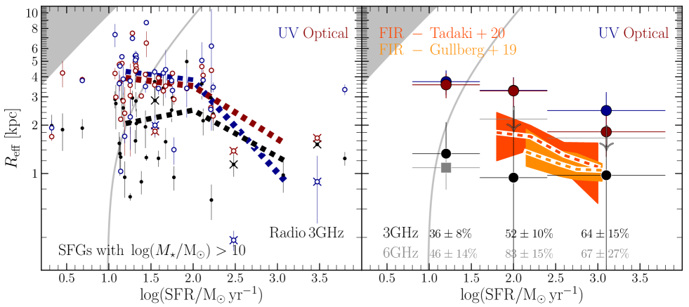
Figure 10: Left panel– The radio/UV/optical effective radius of $\log(M_{\star}/\rm M_{\odot})>10$ SFGs that are reliably resolved at 3 GHz as a function of their SFR. The dashed lines show the median effective radius per SFR bin ($1-1.5$ dex width). The cross symbols denote the radio sources with a reported X-ray counterpart. Right panel– The median radio/UV/optical effective radius of all galaxies in the sample (i.e., sources that are reliably and unreliably resolved at 3 GHz) per SFR bin. The dashed lines show the FIR size – SFR relation of 85 massive SFGs at $1.9<z<2.6$ (dark orange; Tadaki et al., 2020) and 163 massive SFGs at $2.5<z<3.5$ (orange; Gullberg et al., 2019). To account for the upper limits to the radio sizes of unreliably resolved galaxies, we derive the median effective radius per stellar mass bin (and its associated uncertainty) via the KM estimator (Kaplan & Meier, 1958). The length of the error bars indicates the error of the median and the stellar mass bin, respectively. The down arrows indicate the upper limit to the median size of galaxies per bin. The grey curve shows the maximum $R_{\rm eff}$ that can be observed for a galaxy at $z=0.9$, which is the median redshift of our galaxy sample. The grey region illustrates the parameter space that can not be probed with our radio data set. The values at the bottom indicate the fraction of unreliably resolved galaxies at 3 and 6 GHz, respectively. In both panels, the radio/UV/optical size of galaxies tend to decrease with SFR. The larger fraction of unreliably resolved galaxies (at both 3 and 6 GHz) with high SFR hints toward the more compact nature of starbursts.

In Figure 10, we also present the UV/optical size – SFR relation for SFGs that are reliably resolved at 3 GHz (left panel) and all SFGs in the sample (i.e., reliably and unreliably resolved; right panel). In both cases, the UV/optical size of galaxies tends to decrease with increasing SFR: galaxies with $\rm SFR\lesssim\rm 10\,M_{\odot}\,yr^{-1}$ are $2.0\pm 0.5$ times more extended than galaxies producing stars at a higher rate (i.e., $\rm SFR\gtrsim\rm 100\,M_{\odot}\,yr^{-1}$, Table 1). These results are consistent with Elbaz et al. (2011) and Wuyts et al. (2011) who derive rest-frame UV and optical sizes, respectively, and show that starbursts are more compact than MS galaxies over the redshift range $0\lesssim z\lesssim 2$.

Despite the apparent trend between the UV/optical size and SFR, we still have to consider whether this result is driven by dust extinction. As we discussed in §3.4.1, dust can dim the UV emission from the galaxy’s central region and, as a result, the apparent UV effective radius is artificially enlarged. Since starbursts host a larger dust content than MS galaxies (Liu et al., 2019), we expect that the (observed) UV effective radius of starbursts tends to be overestimated by a larger fraction. Correcting for this effect would further strengthen the contrast between the UV size of galaxies with low ($\lesssim\rm 10\,M_{\odot}\,yr^{-1}$) and high SFR ($\gtrsim\rm 100\,M_{\odot}\,yr^{-1}$).

Although our radio-selected sample is expected to be dominated by SFGs (§3.1.3), another potential bias affecting the radio size – SFR relation is the contribution from a point-like radio component from an AGN. To address this issue, we exclude the eight AGN candidates (§3.1.3) falling within the SFR bins presented in Figure 10 (left panel). These AGN candidates represent $45\pm 12\%$ of all galaxies in our highest SFR bin, which contrasts with the low fraction ($\lesssim 10\%$) of AGN candidates in the intermediate and lowest SFR bin. By removing such AGN candidates from the analysis, we corroborate that the direction of the radio size – SFR relation presented in Figure 10 is not significantly affected. On the other hand, the median UV/optical size of galaxies in the highest SFR bin becomes uncertain after removing the AGN candidates (see Figure 14). A more statistically significant sample, as well as dedicated multi-wavelength observations to identify AGN-dominated systems, will be needed to verify that the UV/optical size of “pure SFGs” decreases with increasing SFR.

Focusing on the radio size – SFR relation, the apparent compactness of highly active SFGs can also be interpreted within the context of a two-component model. The first component is a compact, dusty starburst ($R_{\rm eff}\sim 1\rm\,kpc$), and the second is a larger ($R_{\rm eff}\sim 5\rm\,kpc$), less active disk (see Gullberg et al., 2019; Thomson et al., 2019). The relative brightness of these two components hence varies as a function of the total SFR of the galaxy. In highly active systems with SFR $\gtrsim 100\,\rm M_{\odot}\,yr^{-1}$, such as Ultra-Luminous Infrared Galaxies (ULIRGS; e.g., Wilson et al., 2014), the small nuclear emission dominates, whereas in more passive galaxies with lower specific SFRs (i.e., SFR/$M_{\star}$) the extended component becomes dominant (Ellison et al., 2018). The effective radius that we measure from the radio, tracing star formation, is thus a weighted sum of these two components, leading to the dependence of $R_{\rm eff}$ on the SFR of galaxies.

The physical mechanisms driving intense star formation in the central component of galaxies have been linked to gas-rich mergers, which channel gas into the center of galaxies and trigger central, compact starbursts (Mihos & Hernquist, 1996; Hopkins et al., 2006). This is the case of local/low-redshift ULIRGS that exhibit high levels of star formation activity (Genzel et al., 2001). However, at high redshifts, galaxies harbor more massive gas reservoirs than their low-redshift counterparts (e.g., Liu et al., 2019; Birkin et al., 2020), potentially rendering violent disk instabilities (VDI) more common and efficient in driving gas inflows (e.g., Bournaud et al., 2007; Bournaud & Elmegreen, 2009; Dekel & Burkert, 2014). This may lead to an abrupt enhancement of the galaxy’s central cold gas surface density, triggering compact starbursts in high-redshift galaxies (Fensch et al., 2017; Wang et al., 2019).

4.4 Size vs redshift

To explore the growth rate of galaxies across cosmic time, we first evaluate our selection function to account for potential biases in deriving the radio/UV/optical size evolution of galaxies. A well-known observational bias is that the most distant galaxies of flux-limited samples tend to be bright sources. As a result, the faint galaxy population is systematically underrepresented at high redshifts. Our radio detection limit of $\approx 4.5\,\rm\mu Jy$ certainly imposes an SFR threshold above which we can detect galaxies of a given SFR and redshift (see Figure 3). Converting this flux density limit into SFR and using the parametrization of the MS from Schreiber et al. (2015), we verify that selecting galaxies in our sample with $\log(M_{\star}/\rm M_{\odot})>10$ (10.5) allow us to probe “typical”, main sequence SFGs out to $z\approx 2$ ($z\approx 3$) (see Figure 3). Hence, by adopting a mass-selection limit of $\log(M_{\star}/\rm M_{\odot})\approx 10$, we are sensitive to both typical and highly active SFGs (starbursts) out to $z\approx 2$. At higher redshifts, $z\gtrsim 2$, our sample is biased toward the starburst population. Although here we present the size evolution of SFGs out to $z\approx 3$ (Figure 11), we acknowledge that the information from our $z=3$ bin is affected by incompleteness, and hence the conclusions drawn from it must be interpreted with caution.

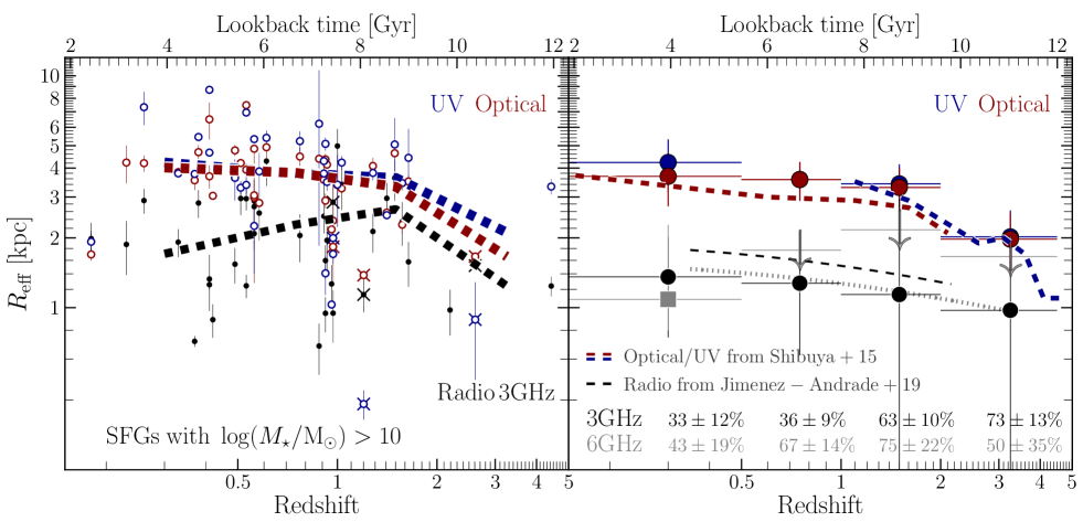
Figure 11: Left panel– Redshift evolution of the radio/UV/optical effective radius of SFGs with $\log(M_{\star}/\rm M_{\odot})>10$ that are reliably resolved at 3 GHz. The dashed lines show the median effective radius per redshift bin ($\approx 2$ Gyr width). The cross symbols denote the radio sources with a reported X-ray counterpart. Right panel– The median radio/UV/optical effective radius of all galaxies in the sample (i.e., sources that are reliably and unreliably resolved at 3 GHz) per redshift bin. The values at the bottom indicate the fraction of unreliably resolved galaxies at 3 and 6 GHz, respectively. The solid black line shows the redshift evolution of the UV/optical size of SFGs with $\log(M_{\star}/{\rm M_{\odot}})=10.5-11$ derived by Shibuya et al. (2015), which is the stellar mass range that resembles the median size of SFGs in our sample ($\log(M_{\star}/{\rm M_{\odot}})=10.6$). The dashed black line shows the redshift evolution of the 3 GHz radio size of ($\log(M_{\star}/{\rm M_{\odot}})>10.5$ SFGs reported by Jiménez-Andrade et al. (2019). The dotted blue line is a fit to the 3 GHz data points presented here, leading to $R_{\rm eff}=(1.6\pm 0.4)(1+z)^{-0.3\pm 0.3}$ kpc. This plot demonstrates that the UV/optical size of massive SFGs is significantly more extended than the 3 GHz radio size out to $z\approx 3$, and that the UV/opitcal/radio size of SFGs with $\log(M_{\star}/\rm M_{\odot})>10$ evolve with redshift at a similar rate.

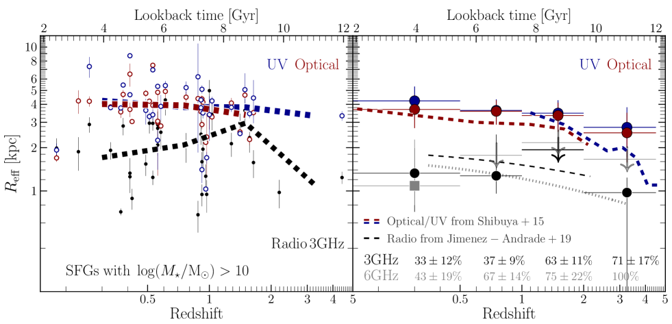
Figure 15: Left panel– Redshift evolution of the radio/UV/optical effective radius of SFGs with $\log(M_{\star}/\rm M_{\odot})>10$ that are reliably resolved at 3 GHz. The dashed lines show the median effective radius per redshift bin ($\approx 2$ Gyr width). Right panel– The median radio/UV/optical effective radius of all galaxies in the sample (i.e., sources that are reliably and unreliably resolved at 3 GHz) per redshift bin. The values at the bottom indicate the fraction of unreliably resolved galaxies at 3 and 6 GHz, respectively. Contrary to the results presented in Figure 10, here we exclude the radio sources that have an X-ray counterpart, which are likely to host an AGN. The dotted blue line is a fit to the 3 GHz data points presented here, leading to $R_{\rm eff}=(1.7\pm 0.4)(1+z)^{-0.5\pm 0.4}$ kpc. A more complete description of this figure can be found in the caption of Figure 11.

In Figure 11, we present the size evolution of SFGs with $\log(M_{\star}/\rm M_{\odot})>10$. In the left panel, we only present SFGs that are reliably resolved at 3 GHz. In the right panel, we show SFGs that are reliably and unreliably resolved at 3 GHz. In both cases, the UV/optical size of SFGs increases by a factor of $2.0\pm 0.4$ from $z\approx 3$ to $z\approx 0.3$ (Table 1, resembling the trend reported by Shibuya et al. (2015) for SFGs with a consistent stellar mass (see right panel of Figure 11). On the contrary, the radio size – redshift relation behaves differently if only SFGs that are reliably resolved at 3 GHz are considered. This is a consequence of the increasing fraction of unresolved galaxies at higher redshifts (right panel of Figure 11). Including only reliably resolved sources in the analysis misses the population of high-redshift, compact radio sources that are not yet resolved in our radio images. We, therefore, rely on the median radio sizes derived via the KM estimator that allow us to consider both reliably and unreliably resolved radio sources (see Table 1). This analysis indicates that the radio size evolution of SFGs in our sample resembles that of massive SFGs reported by Bondi et al. (2018) and Jiménez-Andrade et al. (2019) (see right panel of Figure 11). Qualitatively, we find that the 3 GHz radio size of SFGs evolves with redshift as $R_{\rm eff}=(1.6\pm 0.4)(1+z)^{-0.3\pm 0.3}$ kpc out to $z\approx 3$, which is in agreement with Jiménez-Andrade et al. (2019) who report $R_{\rm eff}=(2.0\pm 0.2)(1+z)^{-0.4\pm 0.1}$ kpc out to $z=2.35$ (see Figure 11). The $\approx$20% lower median 3 GHz size of galaxies in our sample than the one reported by Bondi et al. (2018) and Jiménez-Andrade et al. (2019) is likely a consequence of different selection criteria, as the latter studies consider more massive SFGs with $\log(M_{\star}/\rm M_{\odot})\gtrsim 10.5$ over $0.35<z\lesssim 3$. Lastly, we verify that the radio/UV/optical size evolution of galaxies presented in Figure 11 is not significantly affected if we exclude the 12 AGN candidates in our sample (see Figure 15 in the Appendix).

The radio continuum size evolution of galaxies has been explored at different frequencies. Lindroos et al. (2018) find that the 1.4 GHz radio size of SFGs also decreases with redshift as $R_{\rm eff}\approx 6(1+z)^{-1.7}$ kpc (see their Figure 3). This indicates that the growth rate and radio size at 1.4 GHz are higher than those from the 3 GHz radio emission, possibly due to the frequency-dependent cosmic ray diffusion that leads to more extended radio sizes at lower frequencies (see §4.5). Indeed, the $\approx$1.4 GHz continuum emission can be as extended as the stellar light distribution of $1\lesssim z\lesssim 3$ SFGs (Muxlow et al., 2005; Owen, 2018; Muxlow et al., 2020), while the 10 GHz radio size of galaxies at similar redshifts is always smaller (or equal) than the optical size (Murphy et al., 2017).

The emerging consensus, supported by our observations, is that the $\gtrsim$ 3 GHz radio size of most SFGs remains a factor of three more compact than their optical size out to $z\approx 3$ (Murphy et al., 2017; Bondi et al., 2018; Jiménez-Andrade et al., 2018). Because dust attenuation alone does not seem to account for the large discrepancy between the radio and optical emission of SFGs (see §4.2), our results from Figure 11 suggest that star formation –traced by $\nu\gtrsim 3$ GHz radio continuum imaging – remains centrally concentrated in galaxies across cosmic time. Obtaining reliably dust-corrected UV size of galaxies will be crucial to verify this result (Lang et al., 2019), as it should also trace the centrally enhanced, massive star formation activity revealed by the radio continuum emission.

4.5 The effect of differential cosmic-ray electron diffusion on radio size measurements

Mapping non-thermal (synchrotron) radio emission accelerated by SNRs allows us to trace the sites of massive star formation across galactic disks. However, CREs arising from these SNR can propagate further through the ISM (e.g., Murphy et al., 2008; Murphy, 2009; Murphy et al., 2012a; Berkhuijsen et al., 2013; Kobayashi et al., 2004), biasing to some extent the spatial distribution of star formation in galaxies as traced by radio emission. Because the diffusion length ($l_{\rm diff}$) depends on the CRE emitting frequency and the physical properties of the ISM (e.g., Murphy et al., 2008; Murphy, 2009), here we discuss how CRE diffusion affects the radio size and its dependence on redshift and star formation.

As the redshift increases, our 3 GHz radio imaging probes higher rest-frame frequencies given by $\nu_{\rm em}=3{\rm GHz}(1+z)$. Due to the rapid cooling time (i.e., short lifetime) of high-frequency emitting CRE, these cannot propagate as far as those at lower frequencies. Thus, the more compact radio size of high-redshift galaxies (see Figure 11) might be a consequence of the systematically shorter diffusion length of CRE emitting at $\nu>3{\rm GHz}$. Using the formulae in Murphy et al. (2008, see their Section 7.1), as well as additional considerations for radiative losses, escape and cosmic microwave background (CMB) effects included in Murphy (2009), we estimate the diffusion length of CRE as a function of frequency. This is done by assuming that the propagation of CRE is described by a simple random walk process, the diffusion length can be approximated as $l_{\rm diff}=(\tau_{\rm diff}D_{R})^{1/2}$ (e.g., Murphy et al., 2008; Murphy, 2009; Murphy et al., 2012a); where $D_{R}$ is the rigidity ($R$)-dependent spatial diffusion coefficient and $\tau_{\rm diff}$ is the CRE travel time. $D_{R}=D_{0}[R/{\rm GV}]^{\delta}=D_{0}[(E_{\rm CR}^{2}-E_{0}^{2})^{1/2}/\rm GV]^{\delta}$, where $E_{\rm CR}$ is the CRE energy, $E_{0}$ is the particle rest-mass energy, $D_{0}$ is the normalization constant, and $\delta\sim 0.7$ (Murphy et al., 2012a). Lastly, $\tau_{\rm diff}$ is estimated following Murphy (2009), which takes into account both radiative losses and escape of CREs, along with CMB effects.

Based on these estimates, we find that, at $z\approx 0.3$, the observed 3 GHz radio emission corresponds to CRE emitting at $\nu=4$ GHz, which can diffuse $\approx 1.6$ times further through the ISM than CRE emitting at $\nu=12$ GHz at $z\approx 3$. This observational bias, therefore, could partially account for the $\approx 2$ times larger radio size of galaxies at $z\approx 0.3$ than their high-redshift counterparts at $z\approx 3$. To mitigate the effect of differential CRE diffusion on the radio size evolution of galaxies, we require high-frequency radio observations that probe the thermal (free-free) radiation from massive star-forming regions (e.g., at $\gtrsim$10 GHz; see Murphy et al., 2017).

The age of the CRE populations can also affect the surface brightness distribution, and hence the effective radius, of non-thermal synchrotron emission of galaxies (Murphy et al., 2008). In the case of starbursts, the CRE population is dominated by young, freshly injected particles that have yet to propagate significantly from their birthplaces. Consequently, the non-thermal radio continuum emission can appear more concentrated in starburst galaxies. This physical phenomenon could explain the tentative evidence for more compact radio sizes with increasing star formation activity (see §4.3), as also reported in detail by Jiménez-Andrade et al. (2019). Furthermore, the UV/optical emission also appears more centrally concentrated in starburst galaxies (see Figure 10), also suggesting that the compact radio size of the starbursts reflects a high central SFR surface density that is likely dominated by a population of young, freshly accelerated CREs that yet to propagate significantly into the galaxy disks. Under this scenario, the smaller radio sizes at high redshifts could reflect the increasing contribution from a nuclear starburst relative to a less active, extended disk-like component (Thomson et al., 2019). Verifying this hypothesis will require even deeper and higher resolution radio maps to decompose the surface brightness profile into compact and disk components, as currently done with ALMA observations of the dust continuum with a $\rm FWHM\lesssim 0\farcs 2$ resolution (e.g., Gullberg et al., 2019; Hodge et al., 2019). Decomposing the radio emission profile of high-redshift SFGs will also allow us to trace the assembly of the extended stellar body of the massive SFGs at $z<3$ in our sample, as we expect that these structures might be the remnant of widespread –rather than centrally enhanced– star formation activity across $z>3$ disks.

5 Summary

To better understand the mechanisms driving the stellar mass buildup in star-forming galaxies, we use VLA (Heywood et al.  in press) and HST ACS/WFC3 (Shipley et al., 2018) imaging to measure and compare the rest-frame radio and UV/optical size of 98 star-forming galaxies in the Hubble Frontier Fields. While radio continuum radiation probes the bulk of the massive star formation in galaxies, the optical emission traces the stellar disk of galaxies. Our radio-selected sample comprises 98 star-forming galaxies over $0.3\lesssim z\lesssim 3$, with a median redshift of $z\approx 0.9$ and median stellar mass of $\log(M_{\star}/\rm M_{\odot})\approx 10.4$. Our main results are the following:

• The median 3 GHz radio size for all the 98 galaxies in our sample is $R_{\rm eff}=1.3\pm 0.3$ kpc. Among these, 31 have 6 GHz counterparts. Their median 3 and 6 GHz radio effective radii are $1.3\pm 0.3$ and $1.1^{+0.7}_{-0.3}$ kpc, respectively. This implies a ratio of 3-to-6 GHz radio size of $1.1\pm 0.1$.

• The UV/optical size of galaxies increases with the stellar mass (as widely reported in the literature). In contrast, there is no clear dependence between the 3 GHz radio size and stellar mass of SFGs. Thus, because more massive galaxies are more heavily dust-obscured, it is likely that the UV/optical size – stellar mass relation is partially driven by dust extinction effects.

• The radio size of massive galaxies with $\log(M_{\star}/\rm M_{\odot})>10$ decreases with increasing SFR. SFGs with SFR $\lesssim 10\,\rm M_{\odot}\,yr^{-1}$ are on average $1.5-2.0$ times more extended than the most active systems with SFR $\gtrsim 100\,\rm M_{\odot}\,yr^{-1}$. Removing AGN candidates from the analysis does not significantly affect this result. The median UV/optical size of galaxies with $\log(M_{\star}/\rm M_{\odot})>10$ appears to follow a similar trend, yet it remains unclear if this relation is driven by a higher incidence of AGN in galaxies with SFR $\gtrsim 100\,\rm M_{\odot}\,yr^{-1}$.

• The 3 GHz radio size increases with cosmic time as $R_{\rm eff}/{\rm kpc}\propto(1+z)^{-0.3\pm 0.3}$ across $z\approx 3$ to $z\approx 0.3$. Similarly, the UV/optical size of massive SFGs with $\log(M_{\star}/\rm M_{\odot})>10$ increases by a factor of $2.0\pm 0.4$ from $z\approx 3$ to $z\approx 0.3$. Over the cosmic epoch probed here, the radio size of most SFGs in our radio-selected sample remains a factor of two-to-three more compact than their UV/optical size. This trend appears to be present in the general population of massive SFGs over $0.1\lesssim z\lesssim 1$, which is the redshift range that is not significantly affected by our radio selection function.

Overall, our results indicate that massive, radio-selected SFGs show centrally enhanced star formation activity relative to their outskirts, possibly due to a large concentration of cold gas in the galaxy center generated by VDI- and/or merger-driven gas inflows. The smaller sizes of the most active, radio-selected SFGs suggests that star formation in these galaxies mainly occurs within a central, compact starburst, while less active systems harbor more widespread star formation across the galaxy’s disk. Verifying these trends requires higher-resolution radio observations (FWHM $\lesssim 0\farcs 6$) to decompose the surface brightness profile of radio continuum emission of SFGs into bulge/disk components, as well as dedicated multi-wavelength observations to disentangle the contribution of AGN to the light profile of their host galaxies. Higher frequency radio observations will be paramount as well, as $\gtrsim 10$ GHz radio emission probes the thermal (free-free) radiation that is a better tracer of (instantaneous) massive star formation of $z\gtrsim 1$ galaxies (Murphy et al., 2017).

Appendix A Comparing star formation rate tracers

In this work, we use radio and FUV imaging to trace the dust-obscured and unobscured star formation activity of galaxies in the sample (see §3.2). This information complements existing SFR estimates in the HFF DeepSpace catalog derived via optical-to-near IR (OIR) SED fitting with the fast code (Shipley et al., 2018). Comparing all these distinct SFR tracers is, therefore, relevant to provide scaling relations that allow one to infer extinction-free SFR estimates when only FUV- or OIR-based SFR are available. In Figure 12, we compare our extinction-free radio SFR estimates ($\rm SFR_{3\,GHz}$) with the dust-biased SFR indicators from the FUV-to-OIR regime ($\rm SFR_{FUV}$ and $\rm SFR_{OIR}$). Fitting a linear function to the $\rm SFR_{3\,GHz}-SFR_{FUV}$ relation (in log-log space), we find that

$$\begin{split}\rm\log\left(\frac{SFR_{3\,GHz}}{M_{\odot}\,yr^{-1}}\right)=\rm(0.47\pm 0.07)\log\left(\frac{SFR_{FUV}}{M_{\odot}\,yr^{-1}}\right)+(1.78\pm 0.08),\end{split}$$ (A1)

indicating that $\rm SFR_{3\,GHz}$ and $\rm SFR_{FUV}$ are positively correlated. Yet $\rm SFR_{3\,GHz}$ is on average $\gtrsim 10$ times larger. Similarly, in the $\rm SFR_{3\,GHz}-SFR_{OIR}$ plane we find that

$$\begin{split}\rm\log\left(\frac{SFR_{3\,GHz}}{M_{\odot}\,yr^{-1}}\right)=\rm(0.17\pm 0.04)\log\left(\frac{SFR_{OIR}}{M_{\odot}\,yr^{-1}}\right)+(1.34\pm 0.07).\end{split}$$ (A2)

A Spearman correlation coefficient of only 0.19 and p-value of 0.06 suggest that $\rm SFR_{3\,GHz}$ and $\rm SFR_{OIR}$ are poorly correlated, in addition to the scatter of the relation being $\approx 1$ dex.

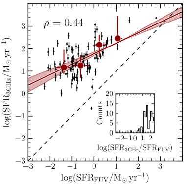
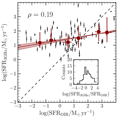
Figure 12: Comparison of the SFR estimated from the 3 GHz radio flux density ($\rm SFR_{3\,GHz}$) with that inferred from the FUV ($\rm SFR_{FUV}$, left panel) and OIR ($\rm SFR_{OIR}$, right panel). The red circles show the median value per SFR bin, while the length of the bars corresponds to their respective 16th/84th percentiles. The dashed black line illustrates the one-to-one relation. The solid red line is the best linear fit to the data points (black circles), whereas the shaded blue region illustrates the uncertainty of such a fit. The inset image shows a histogram of the ordinate to abscissa ratio. The Spearman correlation coefficient, $\rho$, is presented at the upper-left corner of each panel.

Appendix B The multi-wavelength size of galaxies in the HFF

In Table 2, we present the redshift, total SFR, stellar mass, and radio/UV/optical sizes of 98 field galaxies in our sample. We also present the properties of 15 cluster galaxies that are excluded from our analysis. An online version of this table can be found at https://science.nrao.edu/science/surveys/vla-ff/data.

Table 2: The radio/UV/optical size of 98 field (and 15 cluster) galaxies in the HFF.

ID	$z$	$z_{\rm type}$	$\mu$	$\log(M_{\star}/\rm M_{\odot})$	$\rm\log(SFR/M_{\odot}\,yr^{-1})$	$R_{\rm eff}^{\rm UV}$/kpc	$R_{\rm eff}^{\rm opt}$/kpc	$R_{\rm eff}^{\rm 3\,GHz}$/kpc	Res. flag	$R_{\rm eff}^{\rm 6\,GHz}$/kpc	Res. flag	Env.
VLAHFF-J041602.04$-$240523.5	$2.19$	p	$1.66$	$10.14$	$3.07\pm 0.09$	$\dots$	$\dots$	$0.98\pm 0.22$	$\checkmark$	$1.25\pm 0.47$		f
VLAHFF-J041605.30$-$240520.6	$0.39$	s	$1.0$	$11.13$	$0.85\pm 0.1$	$2.62\pm 0.35$	$3.69\pm 0.26$	$1.7\pm 0.38$	$\checkmark$	$\dots$		c
VLAHFF-J041606.36$-$240451.2	$0.74$	s	$3.03$	$10.36$	$1.11\pm 0.16$	$5.71\pm 0.46$	$4.6\pm 0.28$	$0.81\pm 0.36$		$0.0\pm 1.08$		f
VLAHFF-J041606.62$-$240527.8	$1.9$	p	$2.26$	$10.03$	$1.75\pm 0.18$	$\dots$	$\dots$	$1.45\pm 0.49$		$1.55\pm 0.74$		f
VLAHFF-J041607.67$-$240438.7	$0.4$	s	$1.0$	$12.1$	$0.13\pm 0.03$	$3.43\pm 0.27$	$6.81\pm 0.21$	$2.45\pm 0.31$	$\checkmark$	$0.71\pm 0.11$	$\checkmark$	c
VLAHFF-J041607.89$-$240623.4	$0.39$	s	$1.0$	$10.23$	$1.24\pm 0.06$	$3.59\pm 0.09$	$3.85\pm 0.17$	$2.96\pm 0.4$	$\checkmark$	$2.11\pm 0.61$	$\checkmark$	c
VLAHFF-J041608.55$-$240522.0$\,\ast$	$0.97$	s	$1.48$	$10.59$	$1.55\pm 0.14$	$2.0\pm 0.31$	$1.83\pm 0.16$	$2.85\pm 0.63$	$\checkmark$	$\dots$		f
VLAHFF-J041609.11$-$240459.2	$0.71$	s	$1.77$	$9.79$	$0.73\pm 0.17$	$1.88\pm 0.75$	$1.46\pm 0.02$	$0.0\pm 0.84$		$\dots$		f
VLAHFF-J041610.62$-$240407.4	$0.41$	s	$1.06$	$10.35$	$1.13\pm 0.11$	$4.66\pm 0.04$	$3.69\pm 0.42$	$1.33\pm 0.36$	$\checkmark$	$1.46\pm 0.79$		f
VLAHFF-J041610.79$-$240447.5$\,\ast$	$2.09$	s	$1.98$	$9.82$	$2.12\pm 0.14$	$0.4\pm 0.21$	$1.54\pm 0.22$	$1.63\pm 0.62$		$\dots$		f
VLAHFF-J041611.61$-$240221.6	$0.8$	p	$1.16$	$9.69$	$1.26\pm 0.15$	$3.66\pm 0.05$	$3.53\pm 0.05$	$3.04\pm 1.14$		$\dots$		f
VLAHFF-J041611.67$-$240419.6	$2.2$	p	$2.26$	$10.16$	$1.94\pm 0.15$	$3.22\pm 0.31$	$2.54\pm 0.03$	$2.22\pm 0.84$		$\dots$		f
VLAHFF-J041613.23$-$240319.8	$0.91$	s	$1.68$	$10.65$	$1.75\pm 0.08$	$3.79\pm 0.06$	$3.7\pm 0.02$	$2.48\pm 0.39$	$\checkmark$	$2.65\pm 0.81$		f
VLAHFF-J041614.21$-$240359.4	$0.31$	s	$1.0$	$10.54$	$0.43\pm 0.11$	$8.97\pm 0.38$	$7.17\pm 0.44$	$1.27\pm 0.38$		$1.8\pm 0.77$		f
VLAHFF-J041627.72$-$240645.2	$3.27$	p	$1.02$	$9.96$	$2.57\pm 0.17$	$2.17\pm 0.1$	$\dots$	$0.0\pm 1.49$		$\dots$		f
VLAHFF-J041630.23$-$240553.0	$1.59$	p	$1.28$	$10.93$	$1.84\pm 0.16$	$3.51\pm 0.22$	$3.36\pm 0.26$	$0.0\pm 2.03$		$\dots$		f
VLAHFF-J041630.30$-$240630.7	$1.72$	p	$1.13$	$10.29$	$2.12\pm 0.15$	$2.61\pm 0.47$	$2.62\pm 0.07$	$0.0\pm 0.46$		$\dots$		f
VLAHFF-J041636.19$-$240759.7$\,\ast$	$3.55$	p	$1.18$	$12.28$	$3.28\pm 0.13$	$0.29\pm 0.04$	$\dots$	$0.91\pm 0.84$		$\dots$		f
VLAHFF-J041637.88$-$240754.3	$0.51$	s	$0.99$	$10.55$	$1.76\pm 0.12$	$3.29\pm 0.22$	$4.21\pm 0.11$	$2.96\pm 0.45$	$\checkmark$	$\dots$		f
VLAHFF-J041641.49$-$240735.3	$1.95$	p	$1.06$	$10.69$	$2.86\pm 0.13$	$5.13\pm 0.49$	$\dots$	$1.48\pm 0.57$		$\dots$		f
VLAHFF-J041641.59$-$240654.0$\,\ast$	$2.08$	p	$1.23$	$10.71$	$2.76\pm 0.13$	$2.47\pm 0.38$	$\dots$	$1.64\pm 0.63$		$\dots$		f
VLAHFF-J071710.16+375000.9	$0.18$	p	$1.0$	$10.24$	$0.3\pm 0.13$	$2.8\pm 0.01$	$2.77\pm 0.07$	$0.59\pm 0.16$		$\dots$		f
VLAHFF-J071712.40+374946.8	$1.34$	p	$1.1$	$10.31$	$1.88\pm 0.15$	$2.57\pm 7.67$	$2.25\pm 0.14$	$0.0\pm 0.76$		$\dots$		f
VLAHFF-J071715.28+374846.0	$1.13$	p	$1.09$	$10.54$	$1.59\pm 0.15$	$4.52\pm 0.16$	$4.47\pm 0.16$	$3.4\pm 1.14$		$\dots$		f
VLAHFF-J071715.71+374801.3	$0.42$	s	$1.0$	$10.49$	$0.61\pm 0.15$	$3.25\pm 1.31$	$2.78\pm 0.22$	$1.05\pm 0.54$		$\dots$		f
VLAHFF-J071716.05+375108.5	$0.38$	p	$1.0$	$10.94$	$1.32\pm 0.13$	$5.45\pm 0.08$	$4.69\pm 0.34$	$2.83\pm 0.39$	$\checkmark$	$\dots$		f
VLAHFF-J071717.36+374830.4	$1.38$	p	$1.21$	$10.79$	$2.04\pm 0.13$	$6.94\pm 0.31$	$\dots$	$1.23\pm 0.4$		$\dots$		f
VLAHFF-J071717.59+374936.3	$0.54$	s	$1.0$	$10.13$	$1.07\pm 0.14$	$6.73\pm 0.41$	$5.86\pm 0.25$	$1.67\pm 0.51$		$\dots$		f
VLAHFF-J071717.94+374918.0	$1.57$	p	$1.14$	$10.75$	$2.24\pm 0.14$	$3.45\pm 0.24$	$2.28\pm 0.2$	$2.35\pm 0.5$	$\checkmark$	$\dots$		f
VLAHFF-J071718.25+374840.9	$0.68$	s	$1.06$	$11.02$	$1.11\pm 0.15$	$2.16\pm 0.63$	$3.58\pm 0.07$	$0.0\pm 1.13$		$\dots$		f
VLAHFF-J071719.48+374941.4	$1.25$	p	$1.14$	$10.53$	$1.96\pm 0.14$	$2.68\pm 0.31$	$2.88\pm 0.14$	$0.93\pm 0.67$		$\dots$		f
VLAHFF-J071719.99+375054.3$\,\ast$	$0.85$	p	$1.06$	$9.44$	$1.57\pm 0.14$	$0.45\pm 0.06$	$1.98\pm 0.61$	$1.1\pm 0.84$		$\dots$		f
VLAHFF-J071720.14+374956.8	$0.23$	p	$1.0$	$10.69$	$0.45\pm 0.19$	$\dots$	$4.23\pm 0.78$	$1.87\pm 0.49$	$\checkmark$	$\dots$		f
VLAHFF-J071722.31+375107.8$\,\ast$	$1.2$	s	$1.1$	$10.37$	$2.48\pm 0.13$	$0.38\pm 0.06$	$1.38\pm 0.0$	$1.14\pm 0.18$	$\checkmark$	$\dots$		f
VLAHFF-J071723.28+374519.8	$0.42$	s	$1.0$	$10.59$	$1.39\pm 0.06$	$\dots$	$3.04\pm 0.07$	$0.89\pm 0.15$	$\checkmark$	$1.7\pm 0.4$	$\checkmark$	f
VLAHFF-J071723.40+374551.8	$0.47$	p	$1.0$	$10.01$	$0.81\pm 0.14$	$\dots$	$2.15\pm 0.11$	$0.97\pm 0.4$		$\dots$		f
VLAHFF-J071724.84+374352.7	$0.54$	s	$1.0$	$10.01$	$0.97\pm 0.15$	$5.01\pm 0.09$	$4.78\pm 0.1$	$2.27\pm 0.64$	$\checkmark$	$\dots$		c
VLAHFF-J071724.88+374841.3	$1.0$	p	$1.08$	$10.08$	$1.92\pm 0.13$	$3.39\pm 1.16$	$3.38\pm 0.71$	$4.98\pm 0.92$	$\checkmark$	$\dots$		f
VLAHFF-J071724.91+374407.9	$0.54$	s	$1.0$	$10.79$	$1.05\pm 0.14$	$9.33\pm 0.86$	$8.01\pm 0.26$	$1.2\pm 0.39$		$\dots$		c
VLAHFF-J071725.18+374354.1	$0.73$	p	$1.14$	$10.44$	$1.09\pm 0.15$	$3.54\pm 0.22$	$3.05\pm 0.03$	$1.57\pm 0.5$		$\dots$		f
VLAHFF-J071725.83+375018.9$\,\ast$	$2.1$	s	$1.05$	$10.21$	$2.43\pm 0.14$	$0.38\pm 0.11$	$1.97\pm 0.02$	$1.57\pm 0.63$		$\dots$		f
VLAHFF-J071725.85+374446.2	$2.93$	p	$2.21$	$10.36$	$2.16\pm 0.15$	$1.06\pm 0.03$	$\dots$	$1.03\pm 0.52$		$\dots$		f
VLAHFF-J071726.91+374609.2	$0.5$	s	$1.0$	$10.04$	$0.75\pm 0.15$	$2.84\pm 0.12$	$3.0\pm 0.11$	$1.36\pm 0.63$		$\dots$		f
VLAHFF-J071727.21+374605.9	$0.28$	p	$1.0$	$9.82$	$0.72\pm 0.13$	$3.94\pm 0.02$	$3.94\pm 0.07$	$2.04\pm 0.3$	$\checkmark$	$\dots$		f
VLAHFF-J071727.53+374441.2	$0.53$	s	$1.0$	$10.04$	$1.59\pm 0.07$	$3.38\pm 0.29$	$3.93\pm 0.24$	$1.24\pm 0.14$	$\checkmark$	$1.79\pm 0.32$	$\checkmark$	f
VLAHFF-J071728.08+374507.4	$0.61$	p	$1.18$	$10.69$	$1.31\pm 0.13$	$5.4\pm 0.41$	$4.92\pm 0.53$	$4.29\pm 0.94$	$\checkmark$	$\dots$		f
VLAHFF-J071729.06+374320.0	$0.23$	s	$1.0$	$10.56$	$0.04\pm 0.15$	$4.98\pm 2.05$	$3.03\pm 0.4$	$0.54\pm 0.35$		$\dots$		f
VLAHFF-J071729.68+374408.4$\,\ast$	$0.55$	s	$1.0$	$10.77$	$0.77\pm 0.21$	$3.58\pm 0.17$	$3.77\pm 0.03$	$1.87\pm 0.56$	$\checkmark$	$1.41\pm 0.79$		c
VLAHFF-J071729.75+374524.8	$0.56$	s	$1.12$	$10.79$	$1.25\pm 0.14$	$2.25\pm 0.85$	$3.05\pm 1.77$	$2.09\pm 0.33$	$\checkmark$	$\dots$		f
VLAHFF-J071730.39+374617.1	$0.91$	p	$1.81$	$10.62$	$1.54\pm 0.13$	$4.29\pm 0.25$	$3.56\pm 0.16$	$3.73\pm 0.77$	$\checkmark$	$\dots$		f
VLAHFF-J071730.65+374443.1	$1.01$	s	$2.84$	$10.43$	$0.88\pm 0.16$	$3.3\pm 0.14$	$3.33\pm 0.05$	$1.2\pm 0.51$		$\dots$		f
VLAHFF-J071731.51+374437.5	$0.49$	s	$1.0$	$10.9$	$1.12\pm 0.14$	$3.63\pm 0.73$	$4.77\pm 0.26$	$1.54\pm 0.27$	$\checkmark$	$\dots$		f
VLAHFF-J071731.53+374623.8	$0.56$	p	$1.03$	$10.4$	$1.16\pm 0.14$	$5.33\pm 0.13$	$4.85\pm 0.1$	$2.89\pm 0.66$	$\checkmark$	$\dots$		f
VLAHFF-J071731.60+374321.3	$0.22$	p	$1.0$	$9.88$	$0.87\pm 0.04$	$1.56\pm 0.03$	$1.76\pm 0.01$	$0.94\pm 0.07$	$\checkmark$	$1.03\pm 0.15$	$\checkmark$	f
VLAHFF-J071731.75+374333.6	$0.53$	s	$1.0$	$10.29$	$1.28\pm 0.08$	$6.94\pm 0.06$	$7.47\pm 0.17$	$2.95\pm 0.32$	$\checkmark$	$2.29\pm 0.61$	$\checkmark$	f
VLAHFF-J071731.77+374317.2	$0.32$	p	$1.0$	$9.57$	$0.72\pm 0.13$	$2.26\pm 0.02$	$2.43\pm 0.07$	$3.29\pm 0.77$	$\checkmark$	$\dots$		f
VLAHFF-J071732.35+374359.2	$0.53$	s	$1.0$	$9.67$	$1.0\pm 0.15$	$2.27\pm 0.13$	$2.83\pm 0.1$	$3.16\pm 0.96$	$\checkmark$	$\dots$		f
VLAHFF-J071732.39+374319.7	$0.88$	p	$1.25$	$10.42$	$2.22\pm 0.07$	$6.21\pm 4.36$	$4.39\pm 0.07$	$0.68\pm 0.17$	$\checkmark$	$0.0\pm 0.87$		f
VLAHFF-J071733.14+374543.2	$0.91$	s	$2.11$	$9.89$	$1.38\pm 0.14$	$1.36\pm 0.07$	$1.27\pm 0.03$	$2.26\pm 0.47$	$\checkmark$	$\dots$		f
VLAHFF-J071734.46+374432.2	$1.14$	s	$5.84$	$9.42$	$1.56\pm 0.12$	$1.13\pm 0.35$	$2.02\pm 0.14$	$2.69\pm 0.37$	$\checkmark$	$\dots$		f
VLAHFF-J071735.13+374552.7$\,\ast$	$0.55$	s	$1.01$	$10.06$	$0.59\pm 0.18$	$3.75\pm 0.14$	$4.27\pm 0.23$	$0.0\pm 0.34$		$\dots$		c
VLAHFF-J071735.22+374541.7$\,\ast$	$1.69$	s	$3.61$	$10.87$	$1.73\pm 0.14$	$1.38\pm 0.21$	$1.89\pm 0.07$	$0.0\pm 0.24$		$\dots$		f
VLAHFF-J071735.30+374447.3	$0.18$	s	$1.0$	$10.08$	$0.32\pm 0.13$	$1.93\pm 0.21$	$1.7\pm 0.1$	$1.99\pm 0.33$	$\checkmark$	$\dots$		f
VLAHFF-J071735.65+374517.1	$0.54$	s	$1.0$	$12.0$	$1.43\pm 0.09$	$5.17\pm 2.01$	$5.86\pm 0.17$	$0.0\pm 0.05$		$0.74\pm 0.62$		c
VLAHFF-J071736.66+374506.4	$1.13$	s	$6.45$	$9.48$	$1.01\pm 0.15$	$1.8\pm 0.04$	$\dots$	$1.33\pm 0.35$	$\checkmark$	$\dots$		f
VLAHFF-J071737.75+374530.0	$0.55$	s	$1.0$	$9.84$	$1.02\pm 0.14$	$3.33\pm 0.15$	$3.06\pm 0.17$	$1.19\pm 0.34$		$\dots$		c
VLAHFF-J071738.33+374600.0	$0.71$	p	$1.17$	$10.84$	$1.08\pm 0.15$	$3.45\pm 0.98$	$2.21\pm 0.06$	$0.27\pm 1.21$		$1.23\pm 0.66$		f
VLAHFF-J071740.24+374306.5	$1.93$	p	$1.49$	$10.21$	$1.88\pm 0.15$	$0.94\pm 0.09$	$\dots$	$0.0\pm 0.65$		$\dots$		f
VLAHFF-J071740.30+374445.4	$0.55$	s	$1.01$	$9.08$	$1.16\pm 0.15$	$1.79\pm 0.06$	$2.19\pm 0.1$	$2.39\pm 0.52$	$\checkmark$	$\dots$		c
VLAHFF-J071740.55+374506.4$\,\ast$	$1.97$	p	$2.18$	$10.48$	$1.83\pm 0.15$	$\dots$	$\dots$	$0.0\pm 0.51$		$\dots$		f
VLAHFF-J071741.28+374452.1	$0.57$	s	$1.03$	$10.33$	$0.96\pm 0.14$	$3.69\pm 0.07$	$3.35\pm 0.02$	$1.11\pm 0.53$		$\dots$		f
VLAHFF-J071741.56+374555.5	$0.26$	p	$1.0$	$10.84$	$1.07\pm 0.1$	$7.32\pm 1.2$	$4.2\pm 0.34$	$2.9\pm 0.35$	$\checkmark$	$1.13\pm 0.4$		f
VLAHFF-J071742.24+374336.0	$0.54$	s	$1.0$	$11.01$	$1.31\pm 0.15$	$\dots$	$3.92\pm 0.07$	$1.49\pm 0.25$	$\checkmark$	$2.35\pm 0.8$		c
VLAHFF-J071743.17+374651.1	$0.56$	s	$1.01$	$10.37$	$1.08\pm 0.15$	$\dots$	$2.99\pm 0.02$	$2.73\pm 0.84$	$\checkmark$	$\dots$		f
VLAHFF-J114929.44+222314.3	$0.33$	p	$1.0$	$10.1$	$0.69\pm 0.06$	$3.79\pm 0.02$	$3.84\pm 0.17$	$1.92\pm 0.26$	$\checkmark$	$2.28\pm 0.49$	$\checkmark$	f
VLAHFF-J114930.67+222427.7	$1.49$	s	$1.73$	$11.01$	$2.1\pm 0.13$	$5.06\pm 1.51$	$4.64\pm 0.2$	$3.63\pm 0.73$	$\checkmark$	$\dots$		f
VLAHFF-J114930.80+222327.0	$0.37$	s	$1.0$	$10.44$	$1.25\pm 0.04$	$3.77\pm 0.04$	$3.54\pm 0.33$	$0.72\pm 0.04$	$\checkmark$	$0.8\pm 0.08$	$\checkmark$	f
VLAHFF-J114930.83+222253.9	$0.41$	p	$1.0$	$11.01$	$1.45\pm 0.03$	$8.7\pm 0.08$	$6.49\pm 1.18$	$1.26\pm 0.06$	$\checkmark$	$1.09\pm 0.09$	$\checkmark$	f
VLAHFF-J114931.31+222252.1	$0.52$	p	$1.0$	$10.66$	$-0.02\pm 0.07$	$7.13\pm 0.14$	$6.65\pm 0.48$	$0.85\pm 0.29$		$0.82\pm 0.51$		f
VLAHFF-J114932.01+221754.4	$2.16$	p	$0.99$	$10.58$	$2.51\pm 0.14$	$2.77\pm 0.24$	$\dots$	$0.0\pm 0.55$		$\dots$		f
VLAHFF-J114932.03+222439.3	$1.28$	s	$2.11$	$10.19$	$2.12\pm 0.19$	$3.81\pm 0.28$	$4.09\pm 0.34$	$2.13\pm 0.4$	$\checkmark$	$1.52\pm 0.53$		f
VLAHFF-J114933.01+222313.3	$0.56$	s	$1.01$	$9.48$	$0.71\pm 0.08$	$2.58\pm 0.47$	$3.46\pm 0.41$	$1.27\pm 0.27$	$\checkmark$	$4.03\pm 0.83$	$\checkmark$	f
VLAHFF-J114933.14+222430.2	$0.55$	s	$1.08$	$10.68$	$0.63\pm 0.17$	$2.79\pm 0.6$	$3.55\pm 0.09$	$0.0\pm 0.2$		$0.71\pm 0.65$		c
VLAHFF-J114933.57+222321.7	$0.97$	s	$1.46$	$10.03$	$1.19\pm 0.13$	$1.7\pm 0.16$	$2.37\pm 1.08$	$0.95\pm 0.24$	$\checkmark$	$1.78\pm 0.28$	$\checkmark$	f
VLAHFF-J114933.77+222533.2	$1.39$	p	$1.34$	$10.75$	$1.43\pm 0.17$	$2.94\pm 0.65$	$\dots$	$1.02\pm 0.69$		$\dots$		f
VLAHFF-J114933.88+222226.9$\,\ast$	$2.61$	p	$1.22$	$11.66$	$3.47\pm 0.05$	$0.89\pm 0.4$	$1.66\pm 0.01$	$1.52\pm 0.04$	$\checkmark$	$1.66\pm 0.12$	$\checkmark$	f
VLAHFF-J114934.46+222438.5	$0.75$	s	$2.16$	$9.77$	$0.72\pm 0.13$	$2.44\pm 0.15$	$2.84\pm 0.23$	$1.05\pm 0.26$	$\checkmark$	$1.31\pm 0.51$		f
VLAHFF-J114934.65+222320.8	$0.96$	s	$1.53$	$10.43$	$1.14\pm 0.15$	$1.03\pm 2.5$	$2.18\pm 0.04$	$1.27\pm 0.26$	$\checkmark$	$2.64\pm 0.71$	$\checkmark$	f
VLAHFF-J114935.47+222231.9	$0.43$	p	$1.0$	$8.89$	$0.73\pm 0.15$	$3.77\pm 0.11$	$3.4\pm 0.12$	$1.32\pm 0.4$	$\checkmark$	$\dots$		f
VLAHFF-J114936.09+222424.4	$1.64$	p	$3.13$	$10.71$	$1.67\pm 0.15$	$4.43\pm 1.47$	$3.5\pm 0.22$	$1.58\pm 0.35$	$\checkmark$	$\dots$		f
VLAHFF-J114936.83+222253.6	$1.41$	s	$1.6$	$10.32$	$2.21\pm 0.11$	$2.51\pm 0.03$	$2.57\pm 0.02$	$2.96\pm 0.49$	$\checkmark$	$2.36\pm 0.57$	$\checkmark$	f
VLAHFF-J114936.85+222346.9	$0.53$	s	$1.0$	$10.99$	$-0.27\pm 0.19$	$2.96\pm 0.42$	$3.34\pm 0.03$	$0.0\pm 0.93$		$\dots$		c
VLAHFF-J114936.98+222542.0	$0.5$	p	$1.0$	$9.42$	$1.13\pm 0.19$	$4.75\pm 0.12$	$6.59\pm 0.22$	$2.03\pm 0.44$	$\checkmark$	$\dots$		f
VLAHFF-J114937.62+222536.0	$0.52$	p	$1.0$	$9.52$	$1.19\pm 0.08$	$2.56\pm 0.02$	$2.54\pm 0.0$	$1.62\pm 0.23$	$\checkmark$	$1.58\pm 0.5$		f
VLAHFF-J114937.99+222427.7	$0.53$	s	$1.0$	$10.07$	$0.78\pm 0.11$	$7.29\pm 1.54$	$4.04\pm 0.43$	$0.98\pm 0.21$	$\checkmark$	$1.46\pm 0.36$	$\checkmark$	c
VLAHFF-J114938.11+222411.4	$1.03$	s	$1.68$	$10.4$	$1.65\pm 0.13$	$4.22\pm 0.29$	$3.27\pm 0.17$	$3.4\pm 0.76$	$\checkmark$	$\dots$		f
VLAHFF-J114938.62+222145.3	$2.59$	p	$1.2$	$10.62$	$2.36\pm 0.15$	$2.02\pm 0.15$	$\dots$	$1.32\pm 0.46$		$\dots$		f
VLAHFF-J114938.92+222259.8	$0.54$	s	$1.0$	$11.28$	$1.69\pm 0.02$	$3.23\pm 0.71$	$3.9\pm 0.21$	$0.31\pm 0.15$		$0.27\pm 0.09$		c
VLAHFF-J114939.34+222227.3	$0.84$	p	$1.18$	$9.73$	$1.08\pm 0.16$	$4.41\pm 0.15$	$4.0\pm 0.24$	$1.16\pm 0.63$		$\dots$		f
VLAHFF-J114939.73+221856.6	$0.54$	p	$1.0$	$8.74$	$1.09\pm 0.14$	$1.87\pm 0.38$	$1.2\pm 0.17$	$0.44\pm 0.34$		$\dots$		f
VLAHFF-J114939.79+222503.2	$0.92$	p	$1.19$	$10.59$	$1.77\pm 0.13$	$1.41\pm 0.27$	$2.9\pm 0.21$	$0.95\pm 0.16$	$\checkmark$	$0.88\pm 0.36$		f
VLAHFF-J114940.15+222233.3	$0.92$	p	$1.28$	$10.25$	$1.32\pm 0.13$	$5.09\pm 0.33$	$4.36\pm 0.25$	$1.6\pm 0.27$	$\checkmark$	$1.3\pm 0.39$		f
VLAHFF-J114940.57+222415.6	$0.77$	s	$1.18$	$10.24$	$1.33\pm 0.14$	$5.23\pm 0.53$	$4.48\pm 0.39$	$2.05\pm 0.48$	$\checkmark$	$\dots$		f
VLAHFF-J114940.86+222307.4	$0.93$	s	$1.31$	$10.23$	$1.17\pm 0.15$	$3.57\pm 0.31$	$2.87\pm 0.22$	$1.67\pm 0.59$		$\dots$		f
VLAHFF-J114942.38+222339.5	$1.48$	p	$1.36$	$9.73$	$2.13\pm 0.27$	$3.93\pm 0.16$	$\dots$	$1.64\pm 0.32$	$\checkmark$	$1.35\pm 0.49$		f
VLAHFF-J114943.08+221745.0	$1.04$	p	$1.04$	$11.22$	$2.58\pm 0.11$	$7.86\pm 5.0$	$6.57\pm 0.23$	$0.49\pm 0.15$		$0.9\pm 0.59$		f
VLAHFF-J114943.72+222412.8	$0.48$	p	$1.0$	$9.35$	$1.68\pm 0.11$	$3.33\pm 0.01$	$3.67\pm 0.11$	$2.38\pm 0.33$	$\checkmark$	$1.34\pm 0.43$		f
VLAHFF-J114944.33+222408.6	$0.93$	p	$1.09$	$10.07$	$1.44\pm 0.25$	$3.49\pm 0.29$	$4.14\pm 0.01$	$1.95\pm 0.51$	$\checkmark$	$1.53\pm 0.69$		f
VLAHFF-J114945.47+221700.4	$4.43$	p	$1.03$	$11.55$	$3.8\pm 0.13$	$3.33\pm 0.25$	$\dots$	$1.24\pm 0.12$	$\checkmark$	$\dots$		f
VLAHFF-J114945.73+222419.0	$0.58$	p	$1.01$	$10.08$	$1.17\pm 0.14$	$3.87\pm 0.78$	$2.83\pm 0.04$	$2.56\pm 0.61$	$\checkmark$	$\dots$		f
VLAHFF-J114948.03+221907.2	$2.16$	p	$1.24$	$9.8$	$2.22\pm 0.16$	$1.98\pm 0.1$	$\dots$	$0.86\pm 0.59$		$\dots$		f
VLAHFF-J114948.12+221830.6	$0.75$	p	$1.08$	$10.47$	$1.36\pm 0.14$	$0.66\pm 0.01$	$1.67\pm 0.02$	$1.39\pm 0.42$		$\dots$		f
VLAHFF-J114949.00+221803.2	$2.77$	p	$1.39$	$10.62$	$2.42\pm 0.16$	$\dots$	$\dots$	$0.0\pm 0.78$		$\dots$		f

Appendix C The impact of AGN candidates in the size – SFR, stellar mass, and redshift relations.

Out of 113 galaxies in our sample, 12 have an X-ray counterpart with a luminosity $L_{\rm X}>10^{42}\rm\,erg\,s^{-1}$. Thus, it is likely that the radio emission from these galaxies have some potential contribution from an AGN (§3.1.3). By removing the 12 AGN candidates from the analysis, we find that the radio size – SFR, stellar mass, and redshift relations (Figure 13, 14, 15) are consistent with the trends derived from the full galaxy sample (Figure 9, 10, 11). The only exception is the median UV/optical size of galaxies in our highest SFR bin, which is strongly affected by small-number statistics after removing the AGN candidates from the sample.

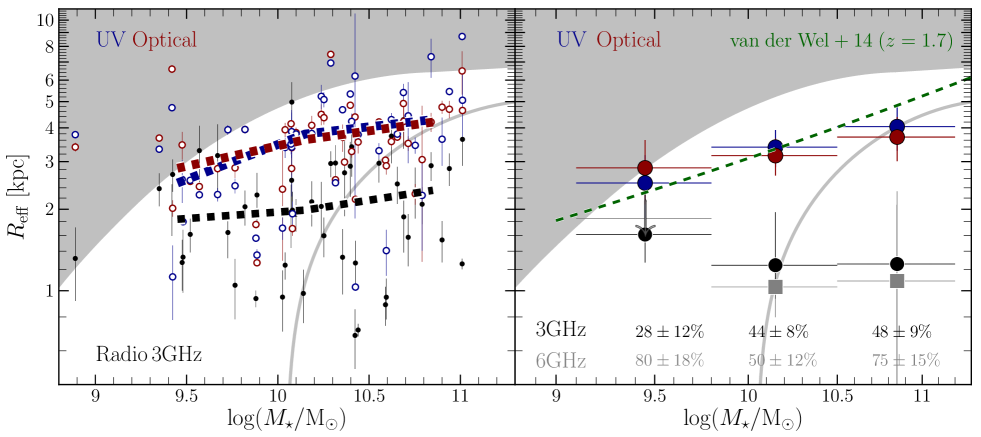
Figure 13: Left panel– The radio/UV/optical effective radius of galaxies that are reliably resolved at 3 GHz as a function of their stellar mass. The dashed lines show the median effective radius per stellar mass bin (0.75 dex width). Right panel– The median radio/UV/optical effective radius of all galaxies in the sample (i.e., sources that are reliably and unreliably resolved at 3 GHz) per stellar mass bin. Contrary to the results presented in Figure 9, here we exclude the radio sources that have an X-ray counterpart, which are likely to host an AGN. A complete description of this figure can be found in the caption of Figure 9.

References

- Abramson & Morishita (2018) Abramson, L. E., & Morishita, T. 2018, ApJ, 858, 40. https://doi.org/10.3847%2F1538-4357%2Faab61b
- Algera et al. (2020) Algera, H. S. B., Smail, I., Dudzevičiūtė, U., et al. 2020, arXiv e-prints, arXiv:2009.06647
- Astropy Collaboration et al. (2013) Astropy Collaboration, Robitaille, T. P., Tollerud, E. J., et al. 2013, A&A, 558, A33
- Astropy Collaboration et al. (2018) Astropy Collaboration, Price-Whelan, A. M., Sipőcz, B. M., et al. 2018, AJ, 156, 123
- Balestra et al. (2016) Balestra, I., Mercurio, A., Sartoris, B., et al. 2016, ApJSS, 224, 33. http://dx.doi.org/10.3847/0067-0049/224/2/33
- Behroozi et al. (2013) Behroozi, P. S., Wechsler, R. H., & Conroy, C. 2013, ApJ, 770, 57. http://dx.doi.org/10.1088/0004-637X/770/1/57
- Bell (2003) Bell, E. F. 2003, ApJ, 586, 794. http://stacks.iop.org/0004-637X/586/i=2/a=794
- Berkhuijsen et al. (2013) Berkhuijsen, E. M., Beck, R., & Tabatabaei, F. S. 2013, MNRAS, 435, 1598
- Birkin et al. (2020) Birkin, J. E., Weiss, A., Wardlow, J. L., et al. 2020, arXiv e-prints, arXiv:2009.03341
- Bondi et al. (2008) Bondi, M., Ciliegi, P., Schinnerer, E., et al. 2008, The Astrophysical Journal, 681, 1129. http://stacks.iop.org/0004-637X/681/i=2/a=1129
- Bondi et al. (2018) Bondi, M., Zamorani, G., Ciliegi, P., et al. 2018, A&A, 618, L8. https://doi.org/10.1051/0004-6361/201834243
- Bonzini et al. (2013) Bonzini, M., Padovani, P., Mainieri, V., et al. 2013, MNRAS, 436, 3759
- Bournaud & Elmegreen (2009) Bournaud, F., & Elmegreen, B. G. 2009, ApJ, 694, L158
- Bournaud et al. (2007) Bournaud, F., Elmegreen, B. G., & Elmegreen, D. M. 2007, ApJ, 670, 237
- Bouwens et al. (2004) Bouwens, R. J., Illingworth, G. D., Blakeslee, J. P., Broadhurst, T. J., & Franx, M. 2004, ApJ, 611, L1. https://doi.org/10.1086%2F423786
- Brammer et al. (2008) Brammer, G. B., van Dokkum, P. G., & Coppi, P. 2008, ApJ, 686, 1503. http://dx.doi.org/10.1086/591786
- Bruzual & Charlot (2003) Bruzual, G., & Charlot, S. 2003, MNRAS, 344, 1000. http://dx.doi.org/10.1046/j.1365-8711.2003.06897.x
- Buat et al. (2012) Buat, V., Noll, S., Burgarella, D., et al. 2012, A&A, 545, A141. https://doi.org/10.1051/0004-6361/201219405
- Calura et al. (2017) Calura, F., Pozzi, F., Cresci, G., et al. 2017, MNRAS, 465, 54. http://dx.doi.org/10.1093/mnras/stw2749
- Calzetti et al. (2000) Calzetti, D., Armus, L., Bohlin, R. C., et al. 2000, ApJ, 533, 682. http://dx.doi.org/10.1086/308692
- Carollo et al. (2013) Carollo, C. M., Bschorr, T. J., Renzini, A., et al. 2013, ApJ, 773, 112. https://doi.org/10.1088%2F0004-637x%2F773%2F2%2F112
- Cerviño et al. (2016) Cerviño, M., Bongiovanni, A., & Hidalgo, S. 2016, A&A, 589, A108. https://www.aanda.org/articles/aa/abs/2016/05/aa28056-15/aa28056-15.html
- Chabrier (2003) Chabrier, G. 2003, PASP, 115, 763. http://stacks.iop.org/1538-3873/115/i=809/a=763
- Chen et al. (2020) Chen, H., Garrett, M. A., Chi, S., et al. 2020, A&A, 638, A113
- Condon (1992) Condon, J. J. 1992, ARA&A, 30, 575
- Condon et al. (1991) Condon, J. J., Huang, Z. P., Yin, Q. F., & Thuan, T. X. 1991, ApJ, 378, 65
- Conselice (2014) Conselice, C. J. 2014, ARA&A, 52, 291. https://doi.org/10.1146/annurev-astro-081913-040037
- Cotton et al. (2018) Cotton, W. D., Condon, J. J., Kellermann, K. I., et al. 2018, ApJ, 856, 67. http://stacks.iop.org/0004-637X/856/i=1/a=67
- Davari et al. (2014) Davari, R., Ho, L. C., Peng, C. Y., & Huang, S. 2014, ApJ, 787, 69. http://dx.doi.org/10.1088/0004-637X/787/1/69
- Davidson-Pilon et al. (2020) Davidson-Pilon, C., Kalderstam, J., Jacobson, N., et al. 2020, CamDavidsonPilon/lifelines: v0.25.6, vv0.25.6, Zenodo, doi:10.5281/zenodo.4136578. https://doi.org/10.5281/zenodo.4136578
- Dekel & Burkert (2014) Dekel, A., & Burkert, A. 2014, MNRAS, 438, 1870. http://dx.doi.org/10.1093/mnras/stt2331
- Dekel et al. (2009) Dekel, A., Birnboim, Y., Engel, G., et al. 2009, Nature, 457, 451. http://dx.doi.org/10.1038/nature07648
- Delhaize et al. (2017) Delhaize, J., Smolčić, V., Delvecchio, I., et al. 2017, A&A, 602, A4. https://doi.org/10.1051/0004-6361/201629430
- Dudzevičiūtė et al. (2020) Dudzevičiūtė, U., Smail, I., Swinbank, A. M., et al. 2020, MNRAS, 494, 3828
- Elbaz et al. (2011) Elbaz, D., Dickinson, M., Hwang, H. S., et al. 2011, A&A, 533, A119. https://doi.org/10.1051/0004-6361/201117239
- Elbaz et al. (2018) Elbaz, D., Leiton, R., Nagar, N., et al. 2018, A&A, 616, A110. https://doi.org/10.1051/0004-6361/201732370
- Ellison et al. (2018) Ellison, S. L., Sánchez, S. F., Ibarra-Medel, H., et al. 2018, MNRAS, 474, 2039. http://dx.doi.org/10.1093/mnras/stx2882
- Evans et al. (2010) Evans, I. N., Primini, F. A., Glotfelty, K. J., et al. 2010, ApJS, 189, 37
- Faisst et al. (2017) Faisst, A. L., Carollo, C. M., Capak, P. L., et al. 2017, ApJ, 839, 71. https://doi.org/10.3847%2F1538-4357%2Faa697a
- Feigelson & Nelson (1985) Feigelson, E. D., & Nelson, P. I. 1985, ApJ, 293, 192
- Fensch et al. (2017) Fensch, J., Renaud, F., Bournaud, F., et al. 2017, MNRAS, 465, 1934. http://dx.doi.org/10.1093/mnras/stw2920
- Ferguson et al. (2004) Ferguson, H. C., Dickinson, M., Giavalisco, M., et al. 2004, ApJ, 600, L107. https://doi.org/10.1086%2F378578
- Florian et al. (2016) Florian, M. K., Li, N., & Gladders, M. D. 2016, ApJ, 832, 168. http://dx.doi.org/10.3847/0004-637X/832/2/168
- Franx et al. (2008) Franx, M., van Dokkum, P. G., Schreiber, N. M. F., et al. 2008, ApJ, 688, 770. https://doi.org/10.1086%2F592431
- Garn et al. (2009) Garn, T., Green, D. A., Riley, J. M., & Alexander, P. 2009, MNRAS, 397, 1101. http://dx.doi.org/10.1111/j.1365-2966.2009.15073.x
- Genzel et al. (2001) Genzel, R., Tacconi, L. J., Rigopoulou, D., Lutz, D., & Tecza, M. 2001, ApJ, 563, 527. http://stacks.iop.org/0004-637X/563/i=2/a=527
- Gim et al. (2019) Gim, H. B., Yun, M. S., Owen, F. N., et al. 2019, ApJ, 875, 80. https://doi.org/10.3847%2F1538-4357%2Fab1011
- González-López et al. (2017) González-López, J., Bauer, F. E., Romero-Cañizales, C., et al. 2017, A&A, 597, A41
- Grazian et al. (2012) Grazian, A., Castellano, M., Fontana, A., et al. 2012, A&A, 547, A51. https://doi.org/10.1051/0004-6361/201219669
- Grillo et al. (2016) Grillo, C., Karman, W., Suyu, S. H., et al. 2016, ApJ, 822, 78. http://dx.doi.org/10.3847/0004-637X/822/2/78
- Gu et al. (2020) Gu, Y., Fang, G., Yuan, Q., & Lu, S. 2020, PASP, in press. arXiv: 2002.11274
- Guidetti et al. (2017) Guidetti, D., Bondi, M., Prandoni, I., et al. 2017, MNRAS, 471, 210. http://dx.doi.org/10.1093/mnras/stx1162
- Gullberg et al. (2019) Gullberg, B., Smail, I., Swinbank, A. M., et al. 2019, MNRAS, 490, 4956
- Habouzit et al. (2019) Habouzit, M., Genel, S., Somerville, R. S., et al. 2019, MNRAS, 484, 4413. https://doi.org/10.1093/mnras/stz102
- Heesen et al. (2014) Heesen, V., Brinks, E., Leroy, A. K., et al. 2014, AJ, 147, 103
- Helou & Bicay (1993) Helou, G., & Bicay, M. D. 1993, ApJ, 415, 93
- Helou et al. (1985) Helou, G., Soifer, B. T., & Rowan-Robinson, M. 1985, ApJL, 298, 7
- Hilz et al. (2012) Hilz, M., Naab, T., Ostriker, J. P., et al. 2012, MNRAS, 425, 3119. https://doi.org/10.1111/j.1365-2966.2012.21541.x
- Hodge et al. (2016) Hodge, J. A., Swinbank, A. M., Simpson, J. M., et al. 2016, ApJ, 833, 103. http://stacks.iop.org/0004-637X/833/i=1/a=103
- Hodge et al. (2019) Hodge, J. A., Smail, I., Walter, F., et al. 2019, ApJ, 876, 130. http://dx.doi.org/10.3847/1538-4357/ab1846
- Hopkins et al. (2006) Hopkins, P. F., Hernquist, L., Cox, T. J., et al. 2006, ApJS, 163, 1
- Huang et al. (2013) Huang, K.-H., Ferguson, H. C., Ravindranath, S., & Su, J. 2013, ApJ, 765, 68. https://doi.org/10.1088%2F0004-637x%2F765%2F1%2F68
- Jauzac et al. (2012) Jauzac, M., Jullo, E., Kneib, J.-P., et al. 2012, MNRAS, 426, 3369
- Jauzac et al. (2014) Jauzac, M., Clément, B., Limousin, M., et al. 2014, MNRAS, 443, 1549
- Jiménez-Andrade et al. (2018) Jiménez-Andrade, E. F., Magnelli, B., Karim, A., et al. 2018, A&A, 615, A25. https://doi.org/10.1051/0004-6361/201732186
- Jiménez-Andrade et al. (2019) Jiménez-Andrade, E. F., Magnelli, B., Karim, A., et al. 2019, A&A, 625, A114. https://doi.org/10.1051/0004-6361/201935178
- Johnson et al. (2014) Johnson, T. L., Sharon, K., Bayliss, M. B., et al. 2014, ApJ, 797, 48. http://dx.doi.org/10.1088/0004-637X/797/1/48
- Kaplan & Meier (1958) Kaplan, E. L., & Meier, P. 1958, Journal of the American Statistical Association, 53, 457. https://www.tandfonline.com/doi/abs/10.1080/01621459.1958.10501452
- Kobayashi et al. (2004) Kobayashi, T., Komori, Y., Yoshida, K., & Nishimura, J. 2004, ApJ, 601, 340. http://stacks.iop.org/0004-637X/601/i=1/a=340
- Kriek et al. (2009) Kriek, M., van Dokkum, P. G., Labbé, I., et al. 2009, ApJ, 700, 221. http://dx.doi.org/10.1088/0004-637X/700/1/221
- Lang et al. (2019) Lang, P., Schinnerer, E., Smail, I., et al. 2019, ApJ, 879, 54. http://dx.doi.org/10.3847/1538-4357/ab1f77
- Laporte et al. (2017) Laporte, N., Bauer, F. E., Troncoso-Iribarren, P., et al. 2017, A&A, 604, A132
- Lequeux (1971) Lequeux, J. 1971, A&A, 15, 42
- Lindroos et al. (2018) Lindroos, L., Knudsen, K. K., Stanley, F., et al. 2018, MNRAS, 476, 3544. http://dx.doi.org/10.1093/mnras/sty426
- Liu et al. (2019) Liu, D., Schinnerer, E., Groves, B., et al. 2019, ApJ, 887, 235. http://dx.doi.org/10.3847/1538-4357/ab578d
- Lotz et al. (2017) Lotz, J. M., Koekemoer, A., Coe, D., et al. 2017, ApJ, 837, 97. http://dx.doi.org/10.3847/1538-4357/837/1/97
- Madau & Dickinson (2014) Madau, P., & Dickinson, M. 2014, ARA&A, 52, 415. https://doi.org/10.1146/annurev-astro-081811-125615
- Magnelli et al. (2015) Magnelli, B., Ivison, R. J., Lutz, D., et al. 2015, A&A, 573, A45. https://doi.org/10.1051/0004-6361/201424937
- Meert et al. (2013) Meert, A., Vikram, V., & Bernardi, M. 2013, MNRAS, 433, 1344
- Miettinen et al. (2017) Miettinen, O., Novak, M., Smolčić, V., et al. 2017, A&A, 602, A54. https://doi.org/10.1051/0004-6361/201730443
- Mihos & Hernquist (1996) Mihos, J. C., & Hernquist, L. 1996, ApJ, 464, 641
- Mohan & Rafferty (2015) Mohan, N., & Rafferty, D. 2015, Astrophysics Source Code Library, 1502.007
- Möllenhoff et al. (2006) Möllenhoff, C., Popescu, C. C., & Tuffs, R. J. 2006, A&A, 456, 941. https://doi.org/10.1051/0004-6361:20054727
- Morishita et al. (2014) Morishita, T., Ichikawa, T., & Kajisawa, M. 2014, ApJ, 785, 18. https://doi.org/10.1088%2F0004-637x%2F785%2F1%2F18
- Mosleh et al. (2013) Mosleh, M., Williams, R. J., & Franx, M. 2013, ApJ, 777, 117. https://doi.org/10.1088%2F0004-637x%2F777%2F2%2F117
- Mosleh et al. (2012) Mosleh, M., Williams, R. J., Franx, M., et al. 2012, ApJL, 756, L12. https://doi.org/10.1088%2F2041-8205%2F756%2F1%2Fl12
- Murphy (2009) Murphy, E. J. 2009, ApJ, 706, 482. http://stacks.iop.org/0004-637X/706/i=1/a=482
- Murphy et al. (2008) Murphy, E. J., Helou, G., Kenney, J. D. P., Armus, L., & Braun, R. 2008, ApJ, 678, 828
- Murphy et al. (2017) Murphy, E. J., Momjian, E., Condon, J. J., et al. 2017, ApJ, 839, 35. http://stacks.iop.org/0004-637X/839/i=1/a=35
- Murphy et al. (2012a) Murphy, E. J., Porter, T. A., Moskalenko, I. V., Helou, G., & Strong, A. W. 2012a, ApJ, 750, 126
- Murphy et al. (2013) Murphy, E. J., Stierwalt, S., Armus, L., Condon, J. J., & Evans, A. S. 2013, ApJ, 768, 2
- Murphy et al. (2006a) Murphy, E. J., Braun, R., Helou, G., et al. 2006a, ApJ, 638, 157. http://stacks.iop.org/0004-637X/638/i=1/a=157
- Murphy et al. (2006b) Murphy, E. J., Helou, G., Braun, R., et al. 2006b, ApJL, 651, L111. http://stacks.iop.org/1538-4357/651/i=2/a=L111
- Murphy et al. (2011) Murphy, E. J., Condon, J. J., Schinnerer, E., et al. 2011, ApJ, 737, 67. https://doi.org/10.1088%2F0004-637x%2F737%2F2%2F67
- Murphy et al. (2012b) Murphy, E. J., Bremseth, J., Mason, B. S., et al. 2012b, ApJ, 761, 97. http://stacks.iop.org/0004-637X/761/i=2/a=97
- Muxlow et al. (2020) Muxlow, A. P., Thomson, J. F., Radcliffe, N. H., et al. 2020, MNRAS, in press.
- Muxlow et al. (2005) Muxlow, T. W. B., Richards, A. M. S., Garrington, S. T., et al. 2005, MNRAS, 358, 1159. http://dx.doi.org/10.1111/j.1365-2966.2005.08824.x
- Nelson et al. (2016) Nelson, E. J., van Dokkum, P. G., Momcheva, I. G., et al. 2016, ApJL, 817, L9. http://stacks.iop.org/2041-8205/817/i=1/a=L9
- Owen (2018) Owen, F. N. 2018, ApJSS, 235, 34. https://doi.org/10.3847%2F1538-4365%2Faab4a1
- Pannella et al. (2015) Pannella, M., Elbaz, D., Daddi, E., et al. 2015, ApJ, 807, 141. http://stacks.iop.org/0004-637X/807/i=2/a=141
- Pastrav et al. (2013) Pastrav, B. A., Popescu, C. C., Tuffs, R. J., & Sansom, A. E. 2013, A&A, 553, A80. https://doi.org/10.1051/0004-6361/201220962
- Paulino-Afonso et al. (2016) Paulino-Afonso, A., Sobral, D., Buitrago, F., & Afonso, J. 2016, MNRAS, 465, 2717. https://doi.org/10.1093/mnras/stw2933
- Rawle et al. (2016) Rawle, T. D., Altieri, B., Egami, E., et al. 2016, MNRAS, 459, 1626. https://doi.org/10.1093/mnras/stw712
- Ribeiro et al. (2016) Ribeiro, B., Le Fèvre, O., Tasca, L. A. M., et al. 2016, A&A, 593. https://doi.org/10.1051/0004-6361/201628249
- Richard et al. (2014) Richard, J., Jauzac, M., Limousin, M., et al. 2014, MNRAS, 444, 268. https://doi.org/10.1093/mnras/stu1395
- Richards (2000) Richards, E. A. 2000, ApJ, 533, 611. http://stacks.iop.org/0004-637X/533/i=2/a=611
- Rodriguez-Gomez et al. (2018) Rodriguez-Gomez, V., Snyder, G. F., Lotz, J. M., et al. 2018, MNRAS, 483, 4140. https://doi.org/10.1093/mnras/sty3345
- Rujopakarn et al. (2016) Rujopakarn, W., Dunlop, J. S., Rieke, G. H., et al. 2016, ApJ, 833, 12. http://stacks.iop.org/0004-637X/833/i=1/a=12
- Salim et al. (2007) Salim, S., Rich, R. M., Charlot, S., et al. 2007, ApJSS, 173, 267. http://stacks.iop.org/0067-0049/173/i=2/a=267
- Sargent et al. (2010) Sargent, M. T., Schinnerer, E., Murphy, E., et al. 2010, ApJSS, 186, 341. http://stacks.iop.org/0067-0049/186/i=2/a=341
- Schinnerer et al. (2010) Schinnerer, E., Sargent, M. T., Bondi, M., et al. 2010, ApJSS, 188, 384. http://dx.doi.org/10.1088/0067-0049/188/2/384
- Schreiber et al. (2015) Schreiber, C., Pannella, M., Elbaz, D., et al. 2015, A&A, 575, A74. https://doi.org/10.1051/0004-6361/201425017
- Shibuya et al. (2015) Shibuya, T., Ouchi, M., & Harikane, Y. 2015, ApJSS, 219, 15. http://stacks.iop.org/0067-0049/219/i=2/a=15
- Shipley et al. (2018) Shipley, H. V., Lange-Vagle, D., Marchesini, D., et al. 2018, ApJSS, 235, 14. http://dx.doi.org/10.3847/1538-4365/aaacce
- Simpson et al. (2015) Simpson, J. M., Smail, I., Swinbank, A. M., et al. 2015, ApJ, 799, 81. http://stacks.iop.org/0004-637X/799/i=1/a=81
- Smolčić et al. (2017a) Smolčić, V., Novak, M., Bondi, M., et al. 2017a, A&A, 602, A1. https://doi.org/10.1051/0004-6361/201628704
- Smolčić et al. (2017b) Smolčić, V., Delvecchio, I., Zamorani, G., et al. 2017b, A&A, 602, A2. https://doi.org/10.1051/0004-6361/201630223
- Steinhardt & Speagle (2014) Steinhardt, C. L., & Speagle, J. S. 2014, ApJ, 796, 25. http://stacks.iop.org/0004-637X/796/i=1/a=25
- Szokoly et al. (2004) Szokoly, G. P., Bergeron, J., Hasinger, G., et al. 2004, ApJSS, 155, 271. http://stacks.iop.org/0067-0049/155/i=2/a=271
- Tacchella et al. (2016) Tacchella, S., Dekel, A., Carollo, C. M., et al. 2016, MNRAS, 457, 2790. http://dx.doi.org/10.1093/mnras/stw131
- Tacchella et al. (2015) Tacchella, S., Carollo, C. M., Renzini, A., et al. 2015, Science, 348, 314. http://science.sciencemag.org/content/348/6232/314
- Tadaki et al. (2018) Tadaki, K., Iono, D., Yun, M. S., et al. 2018, Nature, 560, 613. https://doi.org/10.1038/s41586-018-0443-1
- Tadaki et al. (2020) Tadaki, K.-i., Belli, S., Burkert, A., et al. 2020, ApJ, 901, 74
- Thomson et al. (2019) Thomson, A. P., Smail, I., Swinbank, A. M., et al. 2019, ApJ, 883, 204
- van der Wel et al. (2014) van der Wel, A., Franx, M., van Dokkum, P. G., et al. 2014, ApJ, 788, 28. http://stacks.iop.org/0004-637X/788/i=1/a=28
- van Dokkum et al. (2015) van Dokkum, P. G., Nelson, E. J., Franx, M., et al. 2015, ApJ, 813, 23. https://doi.org/10.1088%2F0004-637x%2F813%2F1%2F23
- van Weeren et al. (2016) van Weeren, R. J., Ogrean, G. A., Jones, C., et al. 2016, ApJ, 817, 98
- van Weeren et al. (2017) —. 2017, ApJ, 835, 197
- Veilleux et al. (2005) Veilleux, S., Cecil, G., & Bland-Hawthorn, J. 2005, ARA&A, 43, 769. https://doi.org/10.1146/annurev.astro.43.072103.150610
- Vika et al. (2015) Vika, M., Vulcani, B., Bamford, S. P., Häußler, B., & Rojas, A. L. 2015, A&A, 577. https://doi.org/10.1051/0004-6361/201425174
- Virtanen et al. (2020) Virtanen, P., Gommers, R., Oliphant, T. E., et al. 2020, Nature Methods, 17, 261
- Wang et al. (2019) Wang, L., De Lucia, G., Fontanot, F., & Hirschmann, M. 2019, MNRAS, 482, 4454
- Wilman et al. (2008) Wilman, R. J., Miller, L., Jarvis, M. J., et al. 2008, MNRAS, 388, 1335
- Wilson et al. (2014) Wilson, C. D., Rangwala, N., Glenn, J., et al. 2014, ApJ, 789, L36
- Wu et al. (2020) Wu, P.-F., van der Wel, A., Bezanson, R., et al. 2020, ApJ, 888, 77. https://doi.org/10.3847%2F1538-4357%2Fab5fd9
- Wuyts et al. (2011) Wuyts, S., Schreiber, N. M. F., van der Wel, A., et al. 2011, ApJ, 742, 96. http://stacks.iop.org/0004-637X/742/i=2/a=96
- Yun et al. (2001) Yun, M. S., Reddy, N. A., & Condon, J. J. 2001, ApJ, 554, 803