Abstract

This chapter describes a novel approach to training machine learning systems by means of a hybrid computer setup i. e. a digital computer tightly coupled with an analog computer. In this example, a reinforcement learning system is trained to balance an inverted pendulum which is simulated on an analog computer, demonstrating a solution to the major challenge of adequately simulating the environment for reinforcement learning.

Chapter 0 Hybrid computer approach to train a machine learning system

1 Introduction

The following sections introduce some basic concepts which underpin the remaining parts of this chapter.

1 A brief introduction to artificial intelligence and machine learning

Machine learning is one of the most exciting technologies of our time. It boosts the range of tasks that computers can perform to a level which has been extremely difficult, if not impossible, to achieve using conventional algorithms.

Thanks to machine learning, computers understand spoken language, offer their services as virtual assistants such as Siri or Alexa, diagnose cancer from magnetic resonance imaging (MRI), drive cars, compose music, paint artistic pictures, and became world champion in the board game Go.

The latter feat is even more impressive when one considers that Go is probably one of the most complex game ever devised; for example it is much more complex than chess. Many observers in 1997 thought that IBM’s Deep Blue, which defeated the then world chess champion Garry Kasparov, was the first proof-of-concept for Artificial Intelligence. However, since chess is a much simpler game than Go, chess-playing computer algorithms can use try-and-error methods to evaluate the best next move from the set of all possible sensible moves. In contrast, due to the $10^{360}$ possible game paths of Go, which is far more than the number of atoms in the universe, it is impossible to use such simple brute-force computer algorithms to calculate the best next move. This is why popular belief stated that it required human intuition, as well as creative and strategic thinking, to master Go – until Google’s AlphaGo beat 18-time world champion Lee Sedol in 2016.

How could AlphaGo beat Lee Sedol? Did Google develop human-like Artificial Intelligence with a masterly intuition for Go and the creative and strategic thinking of a world champion? Far from it. Google’s AlphaGo relied heavily on a machine learning technique called reinforcement learning, RL for short, which is at the center of the novel hybrid analog/digital computing approach introduced in this chapter.

The phrase Artificial Intelligence (AI) on the other hand, is nowadays heavily overused and frequently misunderstood. At the time of writing in early 2020, there exists no AI in the true sense of the word. Three flavors of AI are commonly identified:

Artificial Narrow Intelligence (ANI):

Focused on one narrow task such as playing Go, performing face recognition, or deciding the credit rating of a bank’s customer. Several flavors of machine learning are used to implement ANI.

Artificial General Intelligence (AGI):

Computers with AGI would be equally intelligent to humans in every aspect and would be capable of performing the same kind of intellectual tasks that humans perform with the same level of success. Currently it is not clear if machine learning as we know it today, including Deep Learning, can ever evolve into AGI or if new approaches are required for this.

Artificial Super Intelligence (ASI):

Sometimes called “humanity’s last invention”, ASI is often defined as an intellect that is superior to the best human brains in practically every field, including scientific creativity, general wisdom, and social skills. From today’s perspective, ASI will stay in the realm of science fiction for many years to come.

Machine learning is at the core of all of today’s AI/ANI efforts. Two fundamentally different categories of machine learning can be identified today: The first category, which consists of supervised learning and unsupervised learning, performs its tasks on existing data sets. As described in (Domingos, 2012, p. 85) in the context of Supervised Learning:

“A dumb algorithm with lots and lots of data beats a clever one with modest amounts of it. (After all, machine learning is all about letting data do the heavy lifting.)”

Reinforcement learning constitutes the second category. It is inspired by behaviorist psychology and does not rely on data. Instead, it utilizes the concept of a software agent that can learn to perform certain actions, which depend on a given state of an environment, in order to maximize some kind of long-term (cumulative) reward. Reinforcement learning is very well suited for all kinds of control tasks, as it does not need sub-optimal actions to be explicitly corrected. The focus is on finding a balance between exploration (of uncharted territory) and exploitation (of current knowledge).

Here are some typical applications of machine learning arranged by paradigm:

Supervised learning:

classification (image classification, customer retention, diagnostics) and regression (market forecasting, weather forecasting, advertising popularity prediction)

Unsupervised learning:

clustering (recommender systems, customer segmentation, targeted marketing) and dimensionality reduction (structure discovery, compression, feature elicitation)

Reinforcement learning:

robot navigation, real-time decisions, game AI, resource management, optimization problems

For the sake of completeness, (deep) neural networks need to be mentioned, even though they are not used in this chapter. They are a very versatile family of algorithms that can be used to implement all three of supervised learning, unsupervised learning and reinforcement learning. When reinforcement learning is implemented using deep neural networks then the term deep reinforcement learning is used. The general public often identifies AI or machine learning with neural networks; this is a gross simplification. Indeed there are plenty of other approaches for implementing the different paradigms of machine learning as described in Domingos (2015).

2 Analog vs. digital computing

Analog and digital computers are two fundamentally different approaches to computation. A traditional digital computer, more precisely a stored program digital computer, has a fixed internal structure, consisting of a control unit, arithmetic units etc., which are controlled by an algorithm stored as a program in some kind of memory. This algorithm is then executed in a basically stepwise fashion. An analog computer, in contrast, does not have a memory at all and is not controlled by an algorithm. It consists of a multitude of computing elements capable of executing basic operations such as addition, multiplication, integration (sic!) etc. These computing elements are then interconnected in a suitable way to form an analogue, a model, of the problem to be solved.

So while a digital computer has a fixed internal structure and a variable program controlling its overall operation, an analog computer has a variable structure and no program in the traditional sense at all. The big advantage of the analog computing approach is that all computing elements involved in an actual program are working in full parallelism with no data dependencies, memory bottlenecks etc. slowing down the overall operation.

Another difference is that values within an analog computer are typically represented as voltages or currents and thus are as continuous as possible in the real world. Apart from continuous value representation, analog computers feature integration over time-intervals as one of their basic functions.

When it comes to the solution or simulation of systems described by coupled differential equations, analog computers are much more energy efficient and typically also much faster than digital computers. On the other hand, the generation of arbitrary functions (e. g. functions, which can not be obtained as the solution of some differential equation), complex logic expressions, etc. are hard to implement on an analog computer. So the idea of coupling a digital computer with an analog computer, yielding a hybrid computer, is pretty obvious. The analog computer basically forms a high-performance co-processor for solving problems based on differential equations, while the digital computer supplies initial conditions, coefficients etc. to the analog computer, reads back values and controls the overall operation of the hybrid system.

3 Balancing an inverse pendulum using reinforcement learning

Reinforcement learning is particularly well suited for an analog/digital hybrid approach because the RL agent needs a simulated or real environment in which it can perform, and analog computers excel in simulating multitudes of scenarios. The inverse pendulum, as shown in figure 3, was chosen for the validation of the approach discussed in this chapter because it is one of the classical “Hello World” examples of reinforcement learning and it can be easily simulated on small analog computers.

The hybrid computer setup consists of the analog computer shown in figure 1 that simulates the inverse pendulum and a digital computer running a reinforcement learning algorithm written in Python.

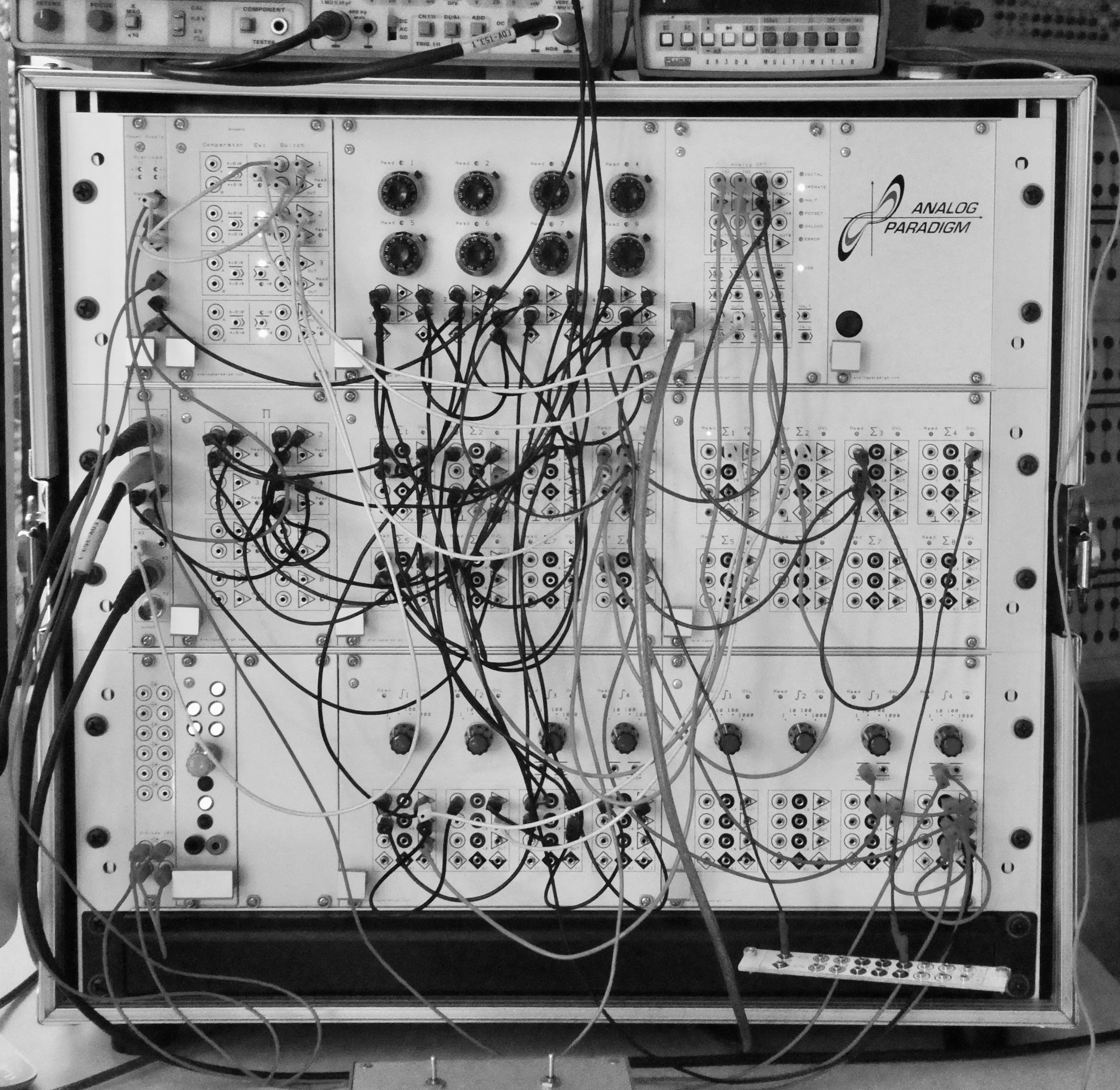
Figure 1: Analog computer setup

Both systems communicate using serial communication over a USB connection. Figure 2 shows the overall setup: The link between the digital computer on the right hand side and the analog computer is a hybrid controller, which controls all parts of the analog computer, such as the integrators, digital potentiometers for setting coefficients etc. This hybrid controller receives commands from the attached digital computer and returns values read from selected computing elements of the analog computer. The simulation and the learning algorithm both run in real-time.

Figure 2: Basic structure of the hybrid computer

Reinforcement learning takes place in episodes. One episode is defined as “balance the pendulum until it falls over or until the cart moves outside the boundaries of the environment”. The digital computer asks the analog computer for real-time simulation information such as the cart’s $x$ position and the pendulum’s angle $\varphi$. The learning algorithm then decides if the current episode, and therefore the current learning process, can continue or if the episode needs to be ended; ending the episode also resets the simulation running on the analog computer.

2 The analog simulation

Simulating an inverted pendulum mounted on a cart with one degree of freedom, as shown in figure 3, on an analog computer is quite straightforward. The pendulum mass $m$ is assumed to be mounted on top of a mass-less pole which in turn is mounted on a pivot on a cart which can be moved along the horizontal axis. The cart’s movement is controlled by applying a force $F$ to the left or right side of the cart for a certain time-interval $\delta t$. If the cart couldn’t move, the pendulum would resemble a simple mathematical pendulum described by

$$\ddot{\varphi}-\frac{g}{l}\sin(\varphi)=0$$

where $\ddot{\varphi}$ is the second derivative of the pendulums angle $\varphi$ with respect to time.

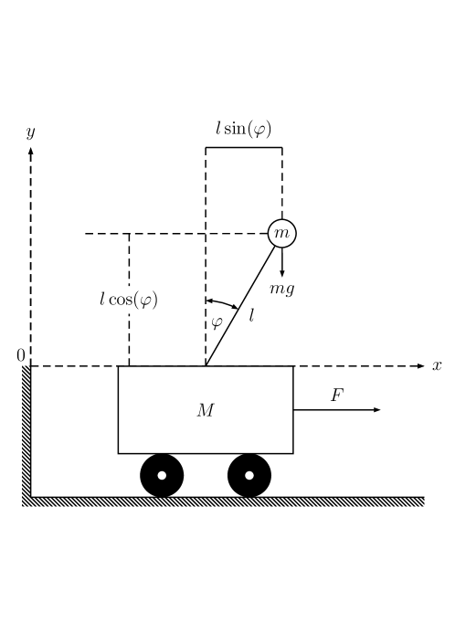
Figure 3: Configuration of the inverted pendulum

Since in this example the cart is non-stationary, the problem is much more complex and another approach has to be taken. In this case, the Lagrangian

$$L=T-V$$

is used, where $T$ and $V$ represent the total kinetic and potential energy of the overall system. With $g$ representing the gravitational acceleration the potential energy is

$$V=mgl\cos(\varphi),$$

the height of the pendulum’s mass above the cart’s upper surface.

The kinetic energy is the sum of the kinetic energies of the pendulum bob with mass $m$ and the moving cart with mass $M$:

$$T=\frac{1}{2}\left(Mv_{c}^{2}+mv_{p}^{2}\right),$$

where $v_{\text{c}}$ and $v_{\text{p}}$ represent the velocities of the cart and the pendulum, respectively. With $x$ denoting the horizontal position of the cart, the cart’s velocity $v_{\text{c}}$ is just the first derivative of its position $x$ with respect to time:

$$v_{\text{c}}=\dot{x}$$

The pendulum’s velocity is a bit more convoluted since the velocity of the pendulum mass has two components, one along the $x$- and one along the $y$-axis forming a two-component vector. The scalar velocity is then the Euclidean norm of this vector, i. e.

$$v_{p}=\sqrt{\left(\frac{\text{d}}{\text{d}t}\left(x-l\sin(\varphi)\right)\right)^{2}+\left(\frac{\text{d}}{\text{d}t}\left(l\cos(\varphi)\right)\right)^{2}}.$$

The two components under the square root are

$$\left(\frac{\text{d}}{\text{d}t}\left(x-l\sin(\varphi)\right)\right)^{2}=\left(\dot{x}-l\dot{\varphi}\cos(\varphi)\right)^{2}=\dot{x}^{2}-2\dot{x}l\dot{\varphi}\cos(\varphi)+l^{2}\dot{\varphi}^{2}\cos^{2}(\varphi)$$

and

$$\left(\frac{\text{d}}{\text{d}t}\left(l\cos(\varphi)\right)\right)^{2}=\left(-l\dot{\varphi}\sin(\varphi)\right)^{2}=l^{2}\dot{\varphi}^{2}\sin^{2}(\varphi)$$

resulting in

$$v_{p} =\dot{x}^{2}-2\dot{x}l\dot{\varphi}\cos(\varphi)+l^{2}\dot{\varphi}^{2}\cos^{2}(\varphi)+l^{2}\dot{\varphi}^{2}\sin^{2}(\varphi)$$

$$=\dot{x}^{2}-2\dot{x}\dot{\varphi}l\cos(\varphi)+l^{2}\dot{\varphi}^{2}.$$

This finally yields the Lagrangian

$$L =\frac{1}{2}M\dot{x}^{2}+\frac{1}{2}\left(\dot{x}^{2}-2\dot{x}\dot{\varphi}l\cos(\varphi)+l^{2}\dot{\varphi}^{2}\right)-mgl\cos{\varphi}$$

$$=\frac{1}{2}(M+m)\dot{x}^{2}+m\dot{x}\dot{\varphi}l\cos(\varphi)+\frac{1}{2}ml^{2}\dot{\varphi}^{2}-mgl\cos(\varphi).$$

As a next step, the Euler-Lagrange-equations

$$\frac{\text{d}}{\text{d}t}\left(\frac{\partial L}{\partial\dot{x}}\right)-\frac{\partial L}{\partial x} =F\text{~{}and}$$ (1)

$$\frac{\text{d}}{\text{d}t}\left(\frac{\partial L}{\partial\dot{\varphi}}\right)-\frac{\partial L}{\partial\varphi} =0$$ (2)

are applied. The first of these equations requires the following partial derivatives

$$\frac{\partial L}{\partial x} =0$$

$$\frac{\partial L}{\partial\dot{x}} =(M+m)\dot{x}-ml\dot{\varphi}\cos(\varphi)$$

$$\frac{\text{d}}{\text{d}t}\left(\frac{\partial L}{\partial\dot{x}}\right) =(M+m)\ddot{x}-ml\ddot{\varphi}\cos(\varphi)+ml\dot{\varphi}^{2}\sin(\varphi)$$

while the second equations relies on these partial derivatives:

$$\frac{\partial L}{\partial\varphi} =ml\dot{x}\dot{\varphi}\sin(\varphi)+mgl\sin(\varphi)$$

$$\frac{\partial L}{\partial\dot{\varphi}} =-ml\dot{x}\cos(\varphi)+ml^{2}\dot{\varphi}$$

$$\frac{\text{d}}{\text{d}t}\left(\frac{\partial L}{\partial\dot{\varphi}}\right) =-ml\ddot{x}\cos(\varphi)+ml\dot{x}\dot{\varphi}\sin(\varphi)+ml^{2}\ddot{\varphi}$$

Substituting these into equations (1) and (2) yields the following two Euler-Lagrange-equations:

$$\frac{\text{d}}{\text{d}t}\left(\frac{\partial L}{\partial\dot{x}}\right)=(M+m)\ddot{x}-ml\ddot{\varphi}\cos(\varphi)+ml\dot{\varphi}^{2}\sin(\varphi)=F$$ (3)

and

$$\frac{\text{d}}{\text{d}t}\left(\frac{\partial L}{\partial\dot{\varphi}}\right)=-ml\ddot{x}\cos(\varphi)+ml\dot{x}\dot{\varphi}\sin(\varphi)+ml^{2}\ddot{\varphi}-ml\dot{x}\dot{\varphi}\sin(\varphi)-mgl\sin(\varphi)=0.$$

Dividing this last equation by $ml$ and solving for $\ddot{\varphi}$ results in

$$\ddot{\varphi}=\frac{1}{l}\left(\ddot{x}\cos(\varphi)+g\sin(\varphi)\right)$$

which can be further simplified to

$$\ddot{\varphi}=\ddot{x}\cos(\varphi)+g\sin(\varphi)$$ (4)

by assuming the pendulum having fixed length $l=1$.

The two final equations of motion (3) and (4) now fully describe the behaviour of the inverted pendulum mounted on its moving cart, to which an external force $F$ may be applied in order to move the cart and therefore the pendulum due to its inertia.

To simplify things further, it can be reasonably assumed that the mass $m$ of the pendulum bob is negligible compared with the cart’s mass $M$, so that (3) can be rewritten as

$$M\ddot{x}=F.$$ (5)

This simplification comes at a cost: the movement of the pendulum bob no longer influences the cart, as it would have been the case with a non-negligible pendulum mass $m$. Nevertheless, this is not a significant restriction and is justified by the the resulting simplification of the analog computer program shown in figure 4.

As stated before, an analog computer program is basically an interconnection scheme specifying how the various computing elements are to be connected to each other. The schematic makes use of several standard symbols:

• Circles with inscribed values represent coefficients. Technically these are basically variable voltage dividers, so a coefficient must always lie in the interval $[0,1]$. The input value $\ddot{x}$ (the force applied to the cart in order to move it on the $x$-axis) is applied to two such voltage dividers, each set to values $\gamma_{1}$ and $\gamma_{2}$.

• Triangles denote summers, yielding the sum of all of its inputs at its output. It should be noted that summers perform an implicit sign inversion, so feeding two values $-h$ and $h\sin(\omega t)$ to a summer as shown in the right half of the schematic, yields an output signal of $-(h\sin(\omega t)-h)=h(1-sin(\omega t))$.

• Symbols labelled with $+\Pi$ denote multipliers while those labelled with $\cos(\dots)$ and $\sin(\dots)$ respectively are function generators.

• Last but not least, there are integrators denoted by triangles with a rectangle attached to one side. These computing elements yield the time integral over the sum of their respective input values. Just as with summers, integrators also perform an implicit sign-inversion.

Transforming the equations of motion (4) and (5) into an analog computer program is typically done by means of the Kelvin feedback technique.

\begin{overpic}[angle={90},width=505.89pt,unit=1mm,tics=10]{pictures/analog_cartpole.pdf} \put(0.5,35.0){$\ddot{x}$} \put(6.0,40.2){$\gamma_{1}$} \put(6.0,28.8){$\gamma_{1}$} \put(14.0,23.0){$\beta_{x}$} \put(16.0,28.0){$-\dot{x}$} \put(26.0,28.0){$x$} \put(33.0,28.0){$-x$} \put(11.0,48.0){$\cos(\varphi)$} \put(20.8,35.8){$g$} \put(32.4,46.4){$\beta_{\varphi}$} \put(23.0,34.0){$\sin(\varphi)$} \put(36.5,40.0){$\dot{\varphi}$} \put(43.5,42.5){$-\varphi$} \put(54.5,45.7){$\cos(\dots)$} \put(54.5,37.1){$\sin(\dots)$} \put(69.3,39.8){$h$} \put(69.3,42.7){$h$} \put(64.2,39.8){$-1$} \put(61.0,42.8){\small$\sin(\omega t)$} \put(99.0,47.7){$y$} \put(99.0,34.0){$x$} \end{overpic}

Figure 4: Modified setup for the inverted pendulum

The tiny analog computer subprogram shown in figure 5 shows how the force applied to the cart is generated in the hybrid computer setup. The circuit is controlled by two digital output signals from the hybrid controller, the interface between the analog computer and its digital counterpart. Activating the output D0 for a short time interval $\delta t$ generates a force impulse resulting in an acceleration $\ddot{x}$ of the cart. The output D1 controls the direction of $\ddot{x}$, thus allowing the cart to be pushed to the left or the right. Both of these control signals are connected to electronic switches which are part of the analog computer.

The outputs of these two switches are then fed to a summer which also takes a second input signal from a manual operated SPDT (single pole double throw) switch. This switch is normally open and makes it possible for an operator to manually disturb the cart, thereby unbalancing the pendulum. It is interesting to see how the RL system responds to such external disturbances.

\begin{overpic}[width=303.53267pt,unit=1mm,tics=10]{pictures/control.pdf} \put(16.0,61.4){\scriptsize push the cart manually} \put(5.5,48.8){$-1$} \put(5.5,54.3){$+1$} \put(0.0,37.7){{D0}} \put(0.0,43.3){{D1}} \put(43.0,60.0){$+1$} \put(43.0,62.7){$-1$} \put(71.0,58.5){$\ddot{x}$} \end{overpic}

Figure 5: Control circuit for the controlled inverted pendulum

3 The reinforcement learning system

Reinforcement learning, as defined in (Sutton, 2018, sec. 1.1),

“is learning what to do — how to map situations to actions — so as to maximize a numerical reward signal. The learner (agent) is not told which actions to take, but instead must discover which actions yield the most reward by trying them. In the most interesting and challenging cases, actions may affect not only the immediate reward but also the next situation and, through that, all subsequent rewards. These two characteristics — trial-and-error search and delayed reward — are the two most important distinguishing features of reinforcement learning.”

In other words, reinforcement learning utilizes the concept of an agent that can learn to perform certain actions depending on a given state of an enivronment in order to maximize some kind of long-term (delayed) reward. Figure 6 illustrates the interplay of the components of a RL system: In each episode, the agent observes the state $s\in\mathbb{S}$ of the system: position $x$ of the cart, speed $\dot{x}$, angle $\varphi$ of the pole and angular velocity $\dot{\varphi}$. Depending on the state, the agent performs an action that modifies the environment. The outcome of the action determines the new state and the short-term reward, which is the main ingredient in finding a value function that is able to predict the long-term reward.

\begin{overpic}[width=260.17464pt,unit=1mm,tics=10]{pictures/rl_basics_wikipedia.jpg} \put(41.5,72.0){Environment} \put(37.0,56.0){\rotatebox{-13.0}{Reward}} \put(6.0,39.0){Interpreter} \put(49.0,5.0){Agent} \put(90.0,45.0){\rotatebox{90.0}{Action}} \end{overpic}

Figure 6: Reinforcement learning

Figure 7 translates these abstract concepts into the concrete use-case of the inverted pendulum. The short-term reward is just a means to an end for finding the value function: Focusing on the short-term reward would only lead to an ever-increasing bouncing of the pendulum, equal to the control algorithm diverging. Instead, using the short-term reward to approximate the value function that can predict the long-term reward leads to a robust control algorithm (convergence).

Figure 7: Rewards in the use-case of the inverted pendulum

1 Value function

Roughly speaking, the state value function $V$ estimates “how benficial” it is to be in a given state. The action value function $Q$ specifies “how beneficial” it is to take a certain action while being in a given state. When it comes for an agent to choose the next best action $a$, one straightforward policy $\pi$ is to evaluate the action value function $Q(s,a)$ for all actions $a$ that are possible while being in state $s$ and to choose the action $a_{\text{best}}$ yielding the maximum value of the action value function:

$$\pi\leftarrow\text{always take}~{}\mathrm{argmax}_{a}(Q(s,a))~{}\text{as next action}$$

A policy like this is also called a greedy policy.

The value function $Q$ for a certain action $a$ given state $s$ is defined as the expected future reward $R$ that can be obtained when the agent is following the current policy $\pi$. The future reward is the sum of the discounted rewards $r$ for each step $t$ beginning from “now” ($s_{0}=s$ at $t=0$) and ranging to the terminal state. $\gamma\in[0,1]$ is implemented as a discount factor by exponentiating it by the number of elapsed steps $t$ in the current training episode.

$$Q(s,a)=E[R(s,a)]=E\Bigg{[}\sum_{t=0}^{\infty}\gamma^{t}r_{t}\Big{|}_{s_{0}=s,a_{0}=a}\Bigg{]}$$

Two important observations regarding the above-mentioned definition of $Q$ are:

1. In step $t=0$ given the state $s_{0}$, the reward $r_{0}$ only depends on the action $a_{0}$. But all subsequent rewards $r_{t}\big{|}_{t>0}$ are depending on all actions that have been previously taken.

2. $\pi$ and $Q(s,a)$ are not defined recursively, but iteratively.

Following the policy $\pi$ as defined here is trivial if $Q$ is given since all that needs to be done in each step is to calculate $\mathrm{argmax}_{a}(Q(s,a))$. So the main challenge of reinforcement learning is to calculate the state value function $V_{\pi}(s)$ and then derive the action value function $Q$ from it or to determine $Q$ directly. But often, $V$ or $Q$ cannot be calculated directly due to CPU or memory constraints. For example the state space $\mathbb{S}=\{(x,\dot{x},\varphi,\dot{\varphi})\in\mathbb{R}^{4}\}$ used here is infinitely large. And even if it is discretized, the resulting combinatorial explosion still results in an enormous state space. So it cannot be expected to find an optimal value function in the limit of finite CPU and memory resources as shown in (Sutton, 2018, Part II). Instead, the goal is to find a good approximate solution that can be calculated relatively quickly.

2 $Q$-learning algorithm

There are several approaches to find the (action) value function $Q$. The implementation described here uses the $Q$-learning algorithm, which is a model-free reinforcement learning algorithm. “Model-free” means, that it actually “does not matter for the algorithm”, what the semantics of the parameters/features of the environment are. It “does not know” the meaning of a feature such as the cart position $x$ or the pole’s angular velocity $\dot{\varphi}$. For the $Q$-learning algorithm, the set of the features $(x,\dot{x},\varphi,\dot{\varphi})$ is just what the current state within the environment comprises. And the state enables the agent to decide which action to perform next.

Chris Watkins introduced $Q$-learning in Watkins (1989) and in (Sutton, 2018, ch. 6). $Q$-learning is defined as a variant of temporal-difference learning (TD):

“TD learning is a combination of Monte Carlo ideas and dynamic programming (DP) ideas. Like Monte Carlo methods, TD methods can learn directly from raw experience without a model of the environment’s dynamics. Like DP, TD methods update estimates based in part on other learned estimates, without waiting for a final outcome (they bootstrap).”

One of the most important properties of $Q$-learning is the concept of explore vs. exploit: The learning algorithm alternates between exploiting what it already knows and exploring unknown territory. Before taking a new action, $Q$-learning evaluates a probability $\varepsilon$ which decides, if the next step is a random move (explore) or if the next move is chosen according to the policy $\pi$ (exploit). As described in section 1, in the context of this chapter the policy $\pi$ is a greedy policy that always chooses the best possible next action, i.e. $\mathrm{argmax}_{a}(Q(s,a))$.

Algorithm 1 $Q$-learning

1:procedure Find_Action_Value_Function_Q

2:     $\alpha\leftarrow\text{step size aka learning rate}\in(0,1]$

3:     $\gamma\leftarrow\text{discount rate}\in(0,1]$

4:     $\varepsilon\leftarrow\text{probability to explore, small and \textgreater~{}0}$

5:     $\text{Initialize}~{}Q(s,a)~{}\forall~{}s\in\mathbb{S},a\in\mathbb{A}(s),\text{arbitrarily}$

6:     $\text{~{}~{}~{}~{}except that}~{}Q(terminal~{}state,\cdot)=0$

7:     Loop for each episode:

8:     Initialize $s$

9:     while $s\neq terminal~{}state$ do

10:         if $random~{}number<\varepsilon$ then

11:              $a\leftarrow\text{random action}\in\mathbb{A}(s)$ $\triangleright$ means: Explore

12:         else

13:              $a\leftarrow\mathrm{argmax}_{a}(Q(s,a))$ $\triangleright$ means: Exploit          

14:         Take action $a$

15:         $r\leftarrow\text{reward for taking action}~{}a~{}\text{while in state}~{}s$

16:         $s^{\prime}\leftarrow\text{state that follows due to taking action}~{}a$

17:         $a_{\text{best}}\leftarrow\mathrm{argmax}_{a}(Q(s^{\prime},a))$

18:          $Q(s,a)\leftarrow Q(s,a)+\alpha[r+\gamma*Q(s^{\prime},a_{\text{best}})-Q(s,a)]$

19:         $s\leftarrow s^{\prime}$      

Algorithm 1 is a temporal difference learner based on Bellman’s equation and is inspired by (Sutton, 2018, sec. 6.5). The state space of the inverse pendulum is denoted as $\mathbb{S}=\{(x,\dot{x},\varphi,\dot{\varphi})\in\mathbb{R}^{4}\}$ and $\mathbb{A}:S\rightarrow 2^{A}$ describes all valid actions for all valid states.

In plain english, the algorithm can be described as follows. For each step within an episode: Decide, if the next action shall explore new territory or exploit knowledge, that has already been learned. After this decision: Take the appropriate action $a$, which means that the reward $r$ for this action is collected and the system enters a new state $s^{\prime}$ (see figure 6). After that: Update the action value function $Q(s,a)$ with an estimated future reward (line 18 of algorithm 1), but discount the estimated future reward with the learning rate $\alpha$.

In machine learning in general the learning rate is a very important parameter, because it makes sure, that new knowledge that has been obtained in the current episode does not completely “overwrite” past knowledge.

The calculation of the estimated future reward is obviously where the magic of $Q$-learning is happening:

$$Q(s,a)\leftarrow Q(s,a)+\alpha[r+\gamma*Q(s^{\prime},a_{\text{best}})-Q(s,a)]$$

$Q$-learning estimates the future reward by taking the short-term reward $r$ for the recently taken action $a$ and adding the discounted delta between the best possible outcome of a hypothetical next action $a_{\text{best}}$ (given the new state $s^{\prime}$) and the old status quo $Q(s,a)$. It is worth mentioning that adding the best possible outcome of $s^{\prime}$ aka $a_{\text{best}}=\mathrm{argmax}_{a}(Q(s^{\prime},a))$ can only be a guess, because it is unclear at the time of this calculation if action $a_{\text{best}}$ is ever being taken due to the “explore vs. exploit” strategy. Still, it seems logical that if $Q(s,a)$ claims to be a measure of “how beneficial” a certain action is, that “the best possible future” $a_{\text{best}}$ from this starting point onwards is then taken into consideration when estimating the future reward.

The discount rate $\gamma$ takes into consideration that the future is not predictable and therefore future rewards cannot be fully counted on. In other words, $\gamma$ is a parameter that balances the RL agent between the two opposite poles “very greedy and short-sighted” and “decision making based on extremely long-term considerations.” As such, $\gamma$ is one of many so called hyper parameters; see also section 3 et seq.

Given the size of $\mathbb{S}$ it becomes clear that many episodes are needed to train a system using $Q$-learning. A rigorous proof that $Q$-learning works and that the algorithm converges is given in Watkins (1992).

When implementing $Q$-learning, a major challenge is how to represent the function $Q(s,a)$. For small to medium sized problems that can be discretized with reasonable effort, tabular representations are appropriate. But as soon as the state space $\mathbb{S}$ is large, as in the case of the inverse pendulum, other representations need to be found.

3 Python implementation

The ideas of this chapter culminate in a hybrid analog/digital machine learning implementation that uses reinforcement learning, more specifically the $Q$-learning algorithm, in conjunction with linear regression, to solve the challenge of balancing the inverse pendulum.

This somewhat arbitrary choice by the authors is not meant to claim that using RL and $Q$-learning is the only or at least optimal way of balancing the inverse pendulum. On the contrary, it is actually more circuitous than many other approaches. Experiments performed by the authors in Python have shown that a simple random search over a few thousand tries yields such $\vec{\theta}=(\theta_{1},\theta_{2},\theta_{3},\theta_{4})$, that the result of the dot-multiplication with the current state of the simulation $\vec{s}=(x,\dot{x},\varphi,\dot{\varphi})$ can reliably decide if the cart should be pushed to the left or to the right, depending, on whether or not $\vec{\theta}\cdot\vec{s}$ is larger than zero.

So the intention of this chapter is something else. The authors wanted to show that a general purpose machine learning algorithm like $Q$-learning, implemented as described in this chapter, is suitable without change for a plethora of other (and much more complex) real world applications and that it can be efficiently trained using a hybrid analog/digital setup.

Python offers a vibrant Open Source ecosystem of building-blocks for machine learning, from which scikit-learn, as described in Pedregosa (2011), was chosen as the foundation of our implementation.

States

Each repetition of the While loop in line 9 of algorithm 1 represents one step within the current iteration. The While loop runs until the current state $s\in\mathbb{S}$ of the inverse pendulum’s simulation reaches a terminal state. This is when the simulation of one episode ends, the simulation is reset and the next episode begins. The terminal state is defined as the cart reaching a certain position $\left|x\right|$ which can be interpreted as “the cart moved too far and leaves the allowed range of movements to the left or to the right or bumps into a wall”. Another trigger for the terminal state is that the angle $\left|\varphi\right|$ of the pole is greater than a certain predefined value, which can be interpreted as “the pole falls over”.

In Python, the state $s\in\mathbb{S}$ is represented as a standard Python Tuple of Floats containing the four elements $(x,\dot{x},\varphi,\dot{\varphi})$ that constitute the state.

During each step of each episode, the analog computer is queried for the current state using the hc_get_sim_state() function (see also sec. 4). On the analog computer, the state is by the nature of analog computers a continuous function. As described in (Wiering, 2012, pp. 3–42) an environment in reinforcement learning is typically stated in the form of a Markov decision process (MDP), because $Q$-learning and many other reinforcement learning algorithms utilize dynamic programming techniques. As an MDP is a discrete time stochastic control process, this means that for the Python implementation, we need to discretize the continuous state representation of the analog computer. Conveniently, this is happening automatically, because the repeated querying inside the While loop mentioned above is nothing else than sampling and therefore a discretization of the continuous (analog) state.

Actions

In theory, one can think of an infinite number of actions that can be performed on the cart on which the inverted pendulum is mounted. As this would complicate the implementation of the $Q$-learning algorithm, the following two simplifications where chosen while implementing actions in Python:

• There are only two possible actions $a\in\{0,1\}$: “Push the cart to the left” and “push the cart to the right”.

• Each action $a$ is allowed in all states $s\in\mathbb{S}$

The actions $a=0$ and $a=1$ are translated to the analog computer simulation by applying a constant force from the right (to push the cart to the left) or the other way round for a defined constant period of time. The magnitude of the force that is being applied is configured as a constant input for the analog computer using a potentiometer, as described in section 2. The constant period of time for which the force is being applied can be configured in the Python software module using HC_IMPULSE_DURATION.

Modeling the action value function $Q(s,a)$

A straightforward way of modeling the action value function in Python could be to store $Q(s,a)$ in a Python Dictionary, so that the Python equivalent of line 18 in algorithm 1 would look like this:

  dictionary.py     1 Q_s_a = {} #create a dictionary to represent Q(s, a) 2  3 [...]      #perform the Q-learning algorithm 4  5 #learn by updating Q(s, a) using learning rate alpha 6 Q_s_a[((x, xdot, phi, phidot), a)] = old_q_s_a + 7                                      alpha * predicted_reward      dictionary.py  

There are multiple problems with this approach, where even the obviously huge memory requirement for trying to store $s\in\mathbb{S}$ in a tabular structure is not the largest one. An even greater problem is that Python’s semantics of Dictionaries are not designed to consider similarities. Instead, they are designated as key-value pairs. For a Python dictionary the two states $s_{1}=(1.0,1.0,1.0,1.0)$ and $s_{2}=(1.0001,1.0,1.0,1.0)$ are completely different and not at all similar. In contrast, for a control algorithm that balances a pendulum, a cart being at x-position $1.0$ is in a very similar situation (state) to a cart being at x-position $1.0001$. So Python’s Dictionaries cannot be used to model $Q(s,a)$. Also, trying to use other tabular methods such as Python’s Lists, creates many other challenges.

This is why linear regression has been chosen to represent and model the function $Q(s,a)$. As we only have two possible states $a\in\{0,1\}$, no general purpose implementation of $Q(s,a)$ has been done. Instead, two discrete functions $Q_{a=0}(s)$ and $Q_{a=1}(s)$ are modeled using a linear regression algorithm from scikit-learn called SGDRegressor, which is capable of performing online learning. In online machine learning, data becomes available step by step and is used to update the best predictor for future data at each step as opposed to batch learning, where the best predictor is generated by using the entire training data set at once.

Given $m$ input features $f_{i}~{}(i=1\dots m)$ and corresponding coefficients $\theta_{i}~{}(i=0\dots m)$, linear regression can predict $\hat{y}$ as follows:

$$\hat{y}=\theta_{0}+\theta_{1}f_{1}+\theta_{2}f_{2}+\dots+\theta_{m}f_{m}$$

The whole point of SGDRegressor is to iteratively refine the values for all $\theta_{i}$, as more and more pairs of $[\hat{y},f_{i}~{}(i=1\dots m)]$ are generated during each step of each episode of the $Q$-learning algorithm with more and more accuracy due to the policy iteration. Older pairs are likely less accurate estimates and are therefore discounted.

A natural choice of features for linear regression would be to set $m=4$ and to use the elements of the state $s\in\mathbb{S}$ as the input features $f$ of the linear regression:

$$Q_{a=n}(s)=\theta_{0}+\theta_{1}x+\theta_{2}\dot{x}+\theta_{3}\varphi+\theta_{4}\dot{\varphi}$$

Experiments performed during the implementation have shown that this choice of features does not produce optimal learning results, as it would lead to underfitting, i.e. the learned model makes too rough predictions for the pendulum to be balanced. The next section 3 explains this phenomenon.

SGDRegressor offers built-in mechanisms to handle the learning rate $\alpha$. When constructing the SGDRegressor object, $\alpha$ can be directly specified as a parameter. Therefore, line 18 of algorithm 1 on page 1 is simplified in the Python implementation, as ”the $\alpha$ used in the $Q$-learning algorithm” and ”the $\alpha$ used inside the SGDRegressor” are semantically identical: The purpose of both of them is to act as the learning rate. Thus, the ”the $\alpha$ used in the $Q$-learning algorithm” can be omitted (means $\alpha$ can be set to $1$):

$$Q_{\text{SGDReg}}(s,a)\leftarrow r+\gamma*Q(s^{\prime},a_{\text{best}})$$

It needs to be mentioned, that the SGDRegressor is not just overwriting the old value with the new value when the above-mentioned formula is executed. Instead, when its online learning function partial_fit is called, it improves the existing predictor for $Q(s,a)$ by using the new value $r+\gamma*Q(s^{\prime},a_{\text{best}})$ discounted by the learning rate $\alpha$.

In plain english, calling partial_fit is equivalent to “the linear regressor that is used to represent $Q(s,a)$ in Python updating its knowledge about the action value function $Q$ for the state $s$ in which action $a$ has been taken by a new estimate without forgetting what has been previously learned. The new estimate that is used to update $Q$ consists of the short-term reward $r$ that came as a result of taking action $a$ while being in step $s$ plus the discounted estimated long-term reward $\gamma*Q(s^{\prime},a_{\text{best}})$ that is obtained by acting as if after action $a$ has been taken, in future always the best possible future action will be taken.”

  analog-cartpole.py     1 # List of possible actions that the RL agent can perform in 2 # the environment. For the algorithm, it doesn’t matter if 0 3 # means right and 1 left or vice versa or if there are more 4 # than two possible actions 5 env_actions = [0, 1] 6  7 [...] 8  9 # we use one Linear Regression per possible action to model 10 # the Value Function for this action, so rbf_net is a list; 11 # SGDRegressor allows step-by-step regression using 12 # partial_fit, which is exactly what we need to learn 13 rbf_net = [SGDRegressor(eta0=ALPHA, 14                         power_t=ALPHA_DECAY, 15                         learning_rate=’invscaling’, 16                         max_iter=5, tol=float("-inf")) 17             for i in range(len(env_actions))] 18  19 [...] 20  21 # learn Value Function for action a in state s 22 def rl_set_Q_s_a(s, a, val): 23     rbf_net[a].partial_fit(rl_transform_s(s), 24                            rl_transform_val(val)) 25  26 [...] 27  28 # Learn the new value for the Value Function 29 new_value = r + GAMMA * max_q_s2a2 30 rl_set_Q_s_a(s, a, new_value)      analog-cartpole.py  

The source snippet shows that there is a regular Python List which contains two objects of type SGDRegressor. Therefore rbf_net[n] can be considered as the representation of $Q_{a=n}(s)$ in memory. For increasing the accuracy of $Q$ during the learning process, the function rl_set_Q_s_a(s, a, val) which itself uses SGDRegressor’s partial_fit function is called regularly at each step of each episode. Therefore lines 29–30 are equivalent to line 18 of algorithm 1.

Feature transformation to avoid underfitting

Underfitting occurs when a statistical model or machine learning algorithm cannot capture the underlying trend of the data. Intuitively, underfitting occurs when the model or the algorithm does not fit the data well enough, because the complexity of the model is too low. As shown in section 2, the inverse pendulum is a non-linear function so one might think that this is the reason that a simple linear regression which tries to match the complexity of a non-linear function using $s\in\mathbb{S}$ as feature set might be prone to underfitting.

In general, this is not the case. As shown at the beginning of this section on page 3 where a control algorithm is introduced, that is based on a randomly found $\vec{\theta}$ and that controls the cart via the linear dot multiplication $\vec{\theta}\cdot\vec{s}$ and where both vectors consist of mere four elements, simple linear functions can absolutely control a complex non-linear phenomenon. So linear control functions per se are not the reason for underfitting.

Instead, the reason why underfitting occurs in the context of the $Q$-learning algorithm is that the very concept of reinforcement learning’s value function, which is a general purpose concept for machine learning, creates overhead and complexity. And this complexity needs to be matched by the statistical model - in our case linear regression - that is chosen to represent $Q(s,a)$. The value function is more complex than a mere control policy like the one that is described on page 3, because it not only contains the information necessary to control the cart but it also contains the information about the expected future reward. This surplus of information needs to be stored somewhere (i.e. needs to be fitted by the model of choice).

The model complexity of linear regression is equivalent to the number $m$ of input features $f_{i}~{}(i=1\dots m)$ in the linear regression equation $\hat{y}=\theta_{0}+\theta_{1}f_{1}+\theta_{2}f_{2}+\dots+\theta_{m}f_{m}$ .

Finding out the optimal threshold of the model complexity necessary to avoid underfitting is a hard task that has not been solved in data science in general at the time of writing. Therefore the model complexity is another one of the many hyper parameters that need to be found and fine-tuned before the actual learning process begins. Finding the right hyper parameters often requires a combination of intuition and trial and error.

Consequently the challenge that had to be solved by the authors was: When the model complexity of linear regression needs to be increased, more features are needed. But how can more than four features be generated, given that $s\in\mathbb{S}$ only consists of the four features $x,\dot{x},\varphi,\dot{\varphi}$?

The solution is to perform a feature transformation, where the number of new features after transforming $s\in\mathbb{S}$ is significantly bigger than four:

$$(x,\dot{x},\varphi,\dot{\varphi})\rightarrow(f_{1},\dots,f_{m})~{}(i=1\dotsm,~{}m>>4)$$

Since the open question here is “how much means significantly?”, one of the requirements for a good feature transformation function is flexibility in the sense that it must be as easy to adjust the hyperparamter “model complexity $m$” as it is to adjust some constants in the Python code (versus finding a completely new feature transformation function each time $m$ needs to be increased or decreased).

It is a best practice of feature engineering that a feature transformation introduces a certain non-linearity. This can be done using many different options such as using a polynomial over the original features.

Radial Basis Functions (RBF) are another option and have been chosen as a means of feature transformation that allows to increase the model complexity $m$ of the linear regression. An RBF is a function that maps a vector to a real number by calculating (usually) the Euclidian distance from the function’s argument to a previously defined center which is sometimes also called an exemplar. This distance is then used inside a kernel function to obtain the output value of the RBF.

By using a large number of RBF transformations, where each RBF uses a different, randomly chosen, center, a high number $m$ of input features $f_{i}$ can be generated for the linear regression. In other words: A feature map of $s$ is generated by applying $m$ different RBFs with $m$ different random centers on $s$:

$$s =(x,\dot{x},\varphi,\dot{\varphi})$$

$$center_{i} =\text{random}(x_{i},\dot{x_{i}},\varphi_{i},\dot{\varphi_{i}})~{}\text{for all}~{}i=1\dots m,$$

$$\delta_{i} =\text{distance}_{euclid_{i}}=\left\lVert(s-center_{i})\right\rVert$$

$$RBF_{i} :s\in\mathbb{S}\rightarrow y_{i}\in\mathbb{R}$$

$$RBF_{i} :e^{-(\beta\delta_{i})^{2}}\rightarrow y_{i}$$ (6)

$\beta$ is a constant for all $i=1\dots m$ that defines the shape of the bell curve described by the Gaussian RBF kernel applied here. So in summary, the method described here is generating $m$ features from the original four features of $s$ where due to the fact that the Eucledian distance to the centers is used, similar states $s$ are yielding similar transformation results $y$. As long as this similarity premise holds and as long as the feature transformation is not just a linear combination of the original features but adds non-linearity, it actually does not matter for the purposes of adding more model complexity to the linear regression, what kind of feature transformation is applied. RBFs are just one example.

Due to the fact that it is beneficial in the context of the analog computer simulation to achieve near real-time performance of the Python software, the above-mentioned RBF transformation has not been implemented verbatim in Python. This would have been too slow. Instead, the scikit-learn class RBFSampler has been used, which generates the feature map of an RBF kernel using a Monte Carlo approximation of its Fourier transform. The experiments have shown that RBFSampler is fast enough and that the approximation is good enough.

  analog-cartpole.py     1 # The following four constants are tunable hyperparameters. 2 # Please note that the source code uses the term GAMMA for 3 # denoting what we are calling BETA in this chapter: The 4 # shape of the bell curve. 5 RBF_EXEMPLARS   = 250  # amount of exemplars per "gamma 6                        # instance" of the RBF network 7 RBF_GAMMA_COUNT = 10   # amount of "gamma instances", i.e. 8                        # RBF_EXEMPLARS*RBF_GAMMA_COUNT feat. 9 RBF_GAMMA_MIN   = 0.05 # minimum gamma, linear interpolation 10                        # between min and max 11 RBF_GAMMA_MAX   = 4.0  # maximum gamma 12  13 [...] 14  15 # create scaler and fit it to the sampled observation space 16 scaler = StandardScaler() 17 scaler.fit(clbr_res) 18  19 [...] 20  21 # the RBF network is built like this: create as many 22 # RBFSamplers as RBF_GAMMA_COUNT and do so by setting the 23 # "width" parameter GAMMA of the RBFs as a linear 24 # interpolation between RBF_GAMMA_MIN and RBF_GAMMA_MAX 25 gammas = np.linspace(RBF_GAMMA_MIN, 26                      RBF_GAMMA_MAX, 27                      RBF_GAMMA_COUNT) 28 models = [RBFSampler(n_components=RBF_EXEMPLARS, 29                      gamma=g) for g in gammas] 30  31 # we will put all these RBFSamplers into a FeatureUnion, so 32 # that our Linear Regression can regard them as one single 33 # feature space spanning over all "Gammas" 34 transformer_list = [] 35 for model in models: 36     # RBFSampler just needs the dimensionality, 37     # not the data itself 38     model.fit([[1.0, 1.0, 1.0, 1.0]]) 39     transformer_list.append((str(model), model)) 40     # union of all RBF exemplar’s output 41     rbfs = FeatureUnion(transformer_list) 42  43 [...] 44  45 # transform the 4 features (Cart Position, Cart Velocity, 46 # Pole Angle and Pole Velocity At Tip) into 47 # RBF_EXEMPLARS*RBF_GAMMA_COUNT distances from the 48 # RBF centers ("Exemplars") 49 def rl_transform_s(s): 50     # during calibration, we do not have a scaler, yet 51     if scaler == None: 52         return rbfs.transform( 53                np.array(s).reshape(1, -1)) 54     else: 55         return rbfs.transform( 56                scaler.transform( 57                np.array(s).reshape(1, -1))) 58  59 # SGDRegressor expects a vector, so we need to transform 60 # our action, which is 0 or 1 into a vector 61 def rl_transform_val(val): 62     return np.array([val]).ravel()      analog-cartpole.py  

Section 3 is missing an explanation for the two functions rl_transform_s and rl_transform_val used in lines 23 and 24 of the source code snippet shown there. The latter one is just a technical necessity, because SGDRegressor expects a vector. In our model, the action is not a vector but an integer, so rl_transform_val ensures, that we transform the integer $a$ into the vector $\vec{a}=\left(a\right)$.

The actual feature transformation is taking place in rl_transform_s. As described above, the scikit-learn class RBFSampler is used for performance reasons. The model complexety $m$ is defined by two constants in Python: RBF_EXEMPLARS and RBF_GAMMA_COUNT and $m$ is the product of both of them. As an enhancement to the formula $RBF_{i}:e^{-(\beta\delta_{i})^{2}}\rightarrow y_{i}$ explained on page 6, where the shape parameter $\beta$ of the Gaussian curve is kept constant, the solution here creates a linear interpolation between the value RBF_GAMMA_MIN and RBF_GAMMA_MAX consisting of RBF_GAMMA_COUNT distinct values for $\beta$. The overall result of $m$ RBF transformations is united in a Python FeatureUnion so that the function rl_transform_s can conveniently call the object rbfs to execute the transformation.

The experiments have shown, that the learning efficiency is higher, when the values that are coming from the analog computer are processed as they are instead of being scaled before. Therefore, the full source code on GitHub (see footnote 17) contains a boolean switch called PERFORM_CALIBRATION that is set to False in the final version. This means, that the if branch shown in lines 48 and 49 is the one performing the feature transformation.

Decaying $\alpha$ and $\varepsilon$ to improve learning and to avoid overfitting

Our experiments have shown that it makes sense to start with relatively high values for the learning rate $\alpha$ and the explore vs. exploit probability $\varepsilon$ and then to decay them over time. This is the equivalent of trying many different options at the beginning when there is still very little knowledge available (high $\varepsilon$ means to favor explore over exploit) and learning quickly from those explorations (high $\alpha$). Later when knowledge has accumulated, it takes more effort to modify facts that have been learned earlier (low $\alpha$).

SGDRegressor has a built in function to decay $alpha$ over time. The $\varepsilon$ decay has been implemented manually. The following code snippet shows the actual parameters used in the implementation.

  analog-cartpole.py     1 GAMMA            = 0.999 # discount factor for Q-learning 2 ALPHA            = 0.6   # initial learning rate 3 ALPHA_DECAY      = 0.1   # learning rate decay 4 EPSILON          = 0.5   # randomness for epsilon-greedy 5 EPSILON_DECAY_t  = 0.1   # decay parameter for epsilon 6 EPSILON_DECAY_m  = 10    # ditto      analog-cartpole.py  

Decaying $\alpha$ and $\varepsilon$ is not only used to improve the learning itself, but also to avoid overfitting the model. Overfitting is described as the “production of an analysis which corresponds too closely or exactly to a particular set of data, and may therefore fail to fit additional data or predict future observations reliably”.

Another mechanism that was used to avoid overfitting is to make sure that the system is “not learning for too long”. The concrete meaning of “too long” is - as many things in machine learning - another hyper parameter. For being able to persistently access the (near to) optimal learning state, the Python implementation supports a command line parameter, that forces the current state of the “brain” to be saved every PROBE episodes, whereas PROBE is a constant (hyper parameter).

4 Hybrid Interface

The Analog Paradigm Model-1 analog computer used by the authors incorporates a Hybrid Controller for connecting the Model-1 to digital computers. It uses an RS232 over USB mechanism that is compatible with most PC operating systems, in the sense that the PC operating system is able to provide a virtual serial port that behaves exactly as if the analog and the digital computer where connected by an RS232 cable instead of an USB cable. This is why, in Python, the communication uses the pySerial library. The following code snippet shows the setup parameters. Note that the Hybrid Controller is communicating at 250,000 baud.

  analog-cartpole.py     1 # Hybrid Controller serial setup 2 HC_PORT             = "/dev/cu.usbserial-DN050L1O" 3 HC_BAUD             = 250000 4 HC_BYTE             = 8 5 HC_PARITY           = serial.PARITY_NONE 6 HC_STOP             = serial.STOPBITS_ONE 7 HC_RTSCTS           = False 8 HC_TIMEOUT          = 2 9  10 [...] 11  12 hc_ser = serial.Serial( port=HC_PORT, 13                         baudrate=HC_BAUD, 14                         bytesize=HC_BYTE, 15                         parity=HC_PARITY, 16                         stopbits=HC_STOP, 17                         rtscts=HC_RTSCTS, 18                         dsrdtr=False, 19                         timeout=HC_TIMEOUT)      analog-cartpole.py  

Analog computers operate in different modes. In this machine learning implementation, the Python script controls the analog computer’s mode of operation according to the needs of the algorithm:

Initial Condition

marks the beginning of an episode. The pendulum is in an upright position.

Operate

is the standard mode of operation, where the analog computer is running the simulation in real-time.

Halt

means that the simulation is paused and that it can be resumed any time by returning to the Operate mode.

The Hybrid Interface accepts certain mode-change commands via the serial line to put the analog computer into the appropriate mode. Moreover, there are several commands to read data from the various computing elements in the analog computer. All the computing elements can be referenced by unique addresses. For being able to influence the calculations of the analog computer, the Hybrid Controller provides analog and digital inputs and outputs. For the purposes of this problem, only two digital outputs are needed to drive the model:

Digital Out #0

is used to set the direction from which the force is being applied when pushing the cart

Digital Out #1

makes sure that a force is applied to the cart as long as it is being set to 1

  analog-cartpole.py     1 # Addresses of the environment/simulation data 2 HC_SIM_X_POS        = "0223" # address cart x 3 HC_SIM_X_VEL        = "0222" # address cart x-velocity 4 HC_SIM_ANGLE        = "0161" # address pendulum angle 5 HC_SIM_ANGLE_VEL    = "0160" # address pend. angular vel. 6  7 HC_SIM_DIRECTION_1  = "D0"   # dout: cart direct. = 1 8 HC_SIM_DIRECTION_0  = "d0"   # dout: cart direct. = 0 9 HC_SIM_IMPULSE_1    = "D1"   # dout: apply force 10 HC_SIM_IMPULSE_0    = "d1"   # dout: apply NO force 11  12 # Model-1 Hybrid Controller: commands 13 HC_CMD_RESET        = "x"    # reset hybrid controller 14 HC_CMD_INIT         = "i"    # initial condition 15 HC_CMD_OP           = "o"    # start to operate 16 HC_CMD_HALT         = "h"    # halt/pause 17 HC_CMD_GETVAL       = "g"    # set address of analog 18                              # computing element and 19                              # return value and ID 20 HC_CMD_BULK_DEFINE  = "G"    # set addresses of multiple 21                              # elements to be returned 22                              # in a bulk transfer via "f" 23 HC_CMD_BULK_FETCH   = "f"    # fetch values of all 24                              # addresses defined by "G" 25 [...] 26  27 def hc_send(cmd): 28     hc_ser.write(cmd.encode("ASCII")) 29  30 def hc_receive(): 31     # HC ends each communication with "\n", 32     #so we can conveniently use readline 33     return hc_ser.readline(). 34                   decode("ASCII"). 35                   split("\n")[0]      analog-cartpole.py  

As described in section 3, the digital computer samples the analog computer’s continuous simulation by repeatedly reading the simulation state variables, to generate the discretization needed for $Q$-learning. The Hybrid Controller supports this effort by providing a bulk readout function that returns the simulation’s overall state with as little overhead as possible. This significantly reduces latency during the learn and control loop, and thus - as experiments have shown - improves the efficiency and convergence speed of the $Q$-learning algorithm.

The bulk mode is activated by sending a bulk definition command that defines a readout group on the Hybrid Controller. After this has been done, the bulk read is triggered by sending a short (single character) fetch command. The following code snippet illustrates the concept and the process.

  analog-cartpole.py     1 #define a readout group in the Hybrid Controller 2 hc_send(HC_CMD_BULK_DEFINE + HC_SIM_X_POS + ’;’ 3                            + HC_SIM_X_VEL + ’;’ 4                            + HC_SIM_ANGLE + ’;’ 5                            + HC_SIM_ANGLE_VEL + ’.’) 6  7 # when using HC_CMD_GETVAL, 8 #HC returns "<value><space><id/type>\n" 9 # we ignore <type> but we expect a well formed response 10 def hc_res2float(str): 11     f = 0 12     try: 13         f = float(str.split(" ")[0]) 14         return f 15     except: 16         [...] 17  18 # query the current state of the simulation, which consists 19 # of the x-pos and the the x-velocity of the cart, the angle 20 # and angle velocity of the pole/pendulum 21 def hc_get_sim_state(): 22     # bulk transfer: ask for all values that consitute the 23     # state in a bulk using a single fetch command 24     if HC_BULK: 25         hc_send(HC_CMD_BULK_FETCH) 26         (res_x_pos, res_x_vel, 27          res_angle, res_angle_vel) = hc_receive().split(’;’) 28         return (hc_res2float(res_x_pos), 29                 hc_res2float(res_x_vel), 30                 hc_res2float(res_angle), 31                 hc_res2float(res_angle_vel)) 32     else: 33         [...]      analog-cartpole.py  

The only way the environment in this example can be influenced by the reinforcement learning agent is via the predefined actions. In this case: “Push the cart to the left or push it to the right.” When looking at this situation from an analog computer’s viewpoint, this is a continuous operation: “To push” means that a force $F$ that does not necessarily need to be constant over time is applied for a certain period of time. As described in section 3 the implementation used here is heavily simplified: Two possible actions, one fixed and constant force $F$ and a constant period of time where the force is applied form the two possible impulses. As the magnitude $\left|F\right|$ of the force is configured directly at the analog computer, the Python code can focus on triggering the impulse using the two above-mentioned digital outputs.

  analog-cartpole.py     1 # duration [ms] of the impulse, that influences the cart 2 HC_IMPULSE_DURATION = 20 3  4 [...] 5  6 # influence simulation by using an impulse to 7 # push the cart to the left or to the right; 8 # it does not matter if "1" means left or right 9 # as long as "0" means the opposite of "1" 10 def hc_influence_sim(a, is_learning): 11     [...] 12  13     if (a == 1): 14         hc_send(HC_SIM_DIRECTION_1) 15     else: 16         hc_send(HC_SIM_DIRECTION_0) 17  18     hc_send(HC_SIM_IMPULSE_1) 19     sleep(HC_IMPULSE_DURATION / 1000.0) 20     hc_send(HC_SIM_IMPULSE_0) 21  22     [...]      analog-cartpole.py  

In summary it can be stated, that working with an analog computer like the Model-1 with its Hybrid Controller is quite straightforward. The serial communication can be encapsulated in some functions or objects and from that moment on, the only thing that one needs to keep in mind is the completely asynchronous and parallel nature of the setup. No assumptions on certain sequence properties can be made and all the typical challenges of asynchronous parallel setups like jitter, race conditions, latency, etc. can occur and need to be managed properly.

4 Results

Analog computers outperform digital computers with respect to raw computational power as well as with respect to power efficiency for certain problems, such as the simulation of dynamic systems that can be readily described by systems of coupled differential equations. This is due to the fact that analog computers are inherently parallel in their operation as they do not rely on some sort of an algorithm being executed in a step-wise fashion. Other advantages are their use of a continuous value representation and that fact that integration is an intrinsic function.

Typical analog computer setups tend to be extremely stable and are not prone to problems like numerical instabilities etc. Although the precision of an analog computer is quite limited compared with a stored-program digital computer employing single or even double precision floating point numbers (a precision analog computer is capable of value representation with about 4 decimal places), solutions obtained by means of an analog computer will always turn out to be realistic, something that cannot be said of numerical simulations where the selection of a suitable integration scheme can have a big effect on the results obtained.

In reinforcement learning scenarios, the actual simulation of the environment as shown in figure 6 on page 6 is one of the hardest and most time consuming things to do. A simulation implemented on an analog computer behaves much more realistically than one performed on a digital computer. It yields unavoidable measurement errors as would be present in a real-world-scenario, it is immune to numerical problems etc.

A plethora of RL algorithms such as (Deep) $Q$-learning are available and well understood, as for example shown in Sutton (2018). Many Open Source implementations are available for free use. So when it comes to practially apply RL to solve challenges in rapidly advancing fields such as autonomous cars, robot navigation, coupling of human nervous signals to artificial limbs and the creation of personalized medical treatments via protein folding, a new project very often starts with the question “how can we simulate the environment for our agent to learn from it?”

The authors have shown in this chapter that this challenge can be very successfully tackled using analog computers, so that a next generation of analog computers based on VLSI analog chips could help to overcome this mainstream challenge of reinforcement learning by propelling the speed and accuracy of environment simulation for RL agents to a new level. This would result in faster development cycles for RL enabled products and therefore could be one of many catalysts in transforming reinforcement learning from a research discipline to an economically viable building block for the truly intelligent device of the future.

References

- Brizard (2008) Alain J. Brizard, An Introduction to Lagrangian Mechanics, World Scientific Publishing Company, 2008
- Domingos (2012) Pedro Domingos, “A Few Useful Things to Know About Machine Learning”, in Communications of the ACM, October 2012, pp. 78–87,
- Domingos (2015) Pedro Domingos, The Master Algorithm: How the Quest for the Ultimate Learning Machine Will Remake Our World, Basic Books, 2015
- Pedregosa (2011) Fabian Pedregosa et al. “Machine Learning in Python”, in Journal of Machine Learning Research Vol. 12, 2011, pp. 2825–2830 doi:10.1145/2347736.2347755
- Sutton (2018) Richard S. Sutton et al., Reinforcement Learning: An Introduction, second edition, The MIT Press, 2018
- Ulmann (2020) Bernd Ulmann, Analog and Hybrid Computer Programming, DeGruyter, 2020
- Watkins (1989) Chris Watkins, Learning from Delayed Rewards, Ph.D. thesis, University of Cambridge, 1989
- Watkins (1992) Chris Watkins, P. Dayan “Q-learning”, in Machine Learning 8(3-4) 1992, pp. 279-292
- Wiering (2012) Marco Wiering et al., Reinforcement Learning, Springer, 2012