Attack as Defense: Characterizing Adversarial Examples using Robustness
Abstract.
As a new programming paradigm, deep learning has expanded its application to many real-world problems. At the same time, deep learning based software are found to be vulnerable to adversarial attacks. Though various defense mechanisms have been proposed to improve robustness of deep learning software, many of them are ineffective against adaptive attacks. In this work, we propose a novel characterization to distinguish adversarial examples from benign ones based on the observation that adversarial examples are significantly less robust than benign ones. As existing robustness measurement does not scale to large networks, we propose a novel defense framework, named attack as defense (A2D), to detect adversarial examples by effectively evaluating an example’s robustness. A2D uses the cost of attacking an input for robustness evaluation and identifies those less robust examples as adversarial since less robust examples are easier to attack. Extensive experiment results on MNIST, CIFAR10 and ImageNet show that A2D is more effective than recent promising approaches. We also evaluate our defence against potential adaptive attacks and show that A2D is effective in defending carefully designed adaptive attacks, e.g., the attack success rate drops to 0% on CIFAR10.
1. Introduction
Deep learning (DL) has arguably become a new programming paradigm which takes over traditional software programs in many areas. For instance, it has achieved state-of-the-art performance in real-world tasks such as autonomous driving (Apollo, ), medical diagnostics (SWS17, ) and cyber-security (SYLS18, ). Despite the success, DL software are still far from dependable (especially for safety- and security-critical systems) and, like traditional software, they must be properly tested, and defended in the presence of malicious inputs. In particular, DL software are known to be brittle to adversarial examples (Intriguing, ; FGSM15, ; CW, ), i.e., by adding a slight perturbation on an input, a well-trained DL model could be easily fooled.
There is a huge body of work proposing various attack and defense mechanisms with regard to adversarial examples, from both the security (FGSM15, ; KGB17, ; JSMA, ; BRB18, ) and software engineering community (wang2019adversarial, ; MJZSXLCSLLZW18, ; TPJR18, ; SWRHKK18, ; Wang2019Dissector, ). Since the adversarial attack L-BFGS was introduced (Intriguing, ), many sophisticated adversarial attacks have been proposed, such as Fast Gradient Sign Method (FGSM) (FGSM15, ), Iterative Gradient Sign Method (BIM) (KGB17, ), Jacobian-based Saliency Map Attack (JSMA) (JSMA, ), Local Search Attack (LSA) (NK17, ), Decision-Based Attack (DBA) (BRB18, ), DeepFool (DeepFool, ), and Carlini and Wagner’s attack (C&W) (CW, ). As countermeasures, defense mechanisms are proposed to improve robustness in the presence of adversarial attacks. Examples include adversarial training (FGSM15, ; MyMSTV17, ; ShafahiNG0DSDTG19, ), defensive distillation (PM0JS16, ) and feature squeezing (Xu0Q18, ). These works constitute important steps in exploring the defense mechanisms, yet have various limitations and are shown to be insufficient (CW, ; HeWCCS17, ; CW17a, ; athalye2018obfuscated, ; TCBM20, ).
Some efforts also have been made to distinguish adversarial examples from benign ones and reject those potentially adversarial ones (wang2019adversarial, ; Wang2019Dissector, ). A usual underlying assumption is that adversarial and benign examples differ in a certain subspace distribution, e.g., kernel density (feinman2017detecting, ), local intrinsic dimensionality (LID, ), manifold (MC17, ), logits values (RothKH19, ), etc. Although these characterizations provide some insights on the adversarial subspace, they are far from reliably discriminating adversarial examples alone. Worse yet, attackers can easily break existing defense mechanisms by specifically designed adaptive attacks (CW17a, ; carlini2017magnet, ; TCBM20, ).
In this work, we propose a novel characterization, i.e., robustness, to distinguish adversarial examples from benign ones. Our main observation is that adversarial examples (crafted by most existing attack methods) are significantly less robust than benign ones. Different from previous statistical characterizations (feinman2017detecting, ; LID, ; MC17, ; RothKH19, ), the difference in robustness comes from two inherent characteristics of model training and adversarial example generation. First, the model training progressively minimizes the loss of each example with respect to the model. Thus, a benign example is often trained to be robust against a model with good generalization. As a result, benign examples are in general relatively far away from the decision boundary. Second, most adversarial attacks aim to generate human-imperceptible perturbations which often result in much less robust just-cross-boundary adversarial examples. The contrasting robustness characteristics make it suitable to distinguish adversarial examples from benign ones.
However, it is still an open research problem on how to effectively measure an input’s robustness with respect to a DL model. Existing robustness measurement methods (e.g., CLEVER (Clever, ) which calculates a minimum perturbation required to change an input’s label) are often too computationally expensive. In this work, we propose to utilize the robustness difference from a reversed angle. Our intuition is that it is easier to employ a successful adversarial attack on an input that is less robust. Thus, we propose a novel defense, named attack as defense (A2D), to effectively detect adversarial examples from benign ones. Given an input example, we apply different kinds of attacks to attack the input and measure how ‘easy’ it is to employ a successful attack. An input example is considered less robust and thus more likely to be adversarial, if the attacks are easier to succeed. Note that the effectiveness of our defense (A2D) relies on a set of attacks whose attack cost (easiness) can be quantitatively measured, which will guide the selection of attacks from a large number of adversarial attacks in the literature.
Compared to existing adversarial example detection approaches (which are mostly proven to be ineffective (athalye2018obfuscated, ; CW, ; CW17a, ; carlini2017magnet, ; HeWCCS17, ; TCBM20, )), our A2D framework has the following advantages. First, A2D utilizes the inherent robustness difference caused by the contrasting characteristics of model training and adversarial example generation. To circumvent the defense, an attack needs to generate robust adversarial examples which in general might induce human-perceptible large distortion. Second, A2D is essentially an ensemble approach using the robustness information obtained from different kinds of attacks which is hard to bypass at once. We evaluated A2D with a carefully selected set of attacks on three popular datasets MNIST (MNIST98, ), CIFAR10 (Kri09, ) and ImageNet (TCBM20, ). Experiment results show that A2D can be more effective than recently proposed detection algorithms (feinman2017detecting, ; LID, ; wang2019adversarial, ; Wang2019Dissector, ) and remain effective even in the white-box adversarial setting. We further show that A2D is effective against adaptive attacks. That is, we show that A2D (combined with a complementary detection approach for detecting large-distortion adversarial examples (MC17, ) and adversarial training) is very effective against specifically designed adaptive attacks, e.g., the attack success rate (ASR) drops from 72% to 0% using our defense with adversarial training on CIFAR10, and the ASR drops from 100% to 0% on MNIST. We remark that many existing defenses combined with adversarial training result in lower robustness than adversarial training on its own (TCBM20, ).
In a nutshell, we make the following contributions:
-
•
We propose a novel characterization to distinguish adversarial examples from benign ones via robustness.
-
•
We present detection approaches based on the characterization, which can utilize existing attacks and do not need to modify or retrain the protected model.
-
•
We conduct extensive experiments to test our observations and our defense, which outperforms recent promising detection algorithms.
-
•
We thoroughly discuss possible adaptive attacks to our defense and evaluate them to our defense integrated with a complementary detection approach and adversarial training. The integrated defense is very promising.
2. Background
2.1. Adversarial Attacks
In this work, we target deep neural network (DNN) for classification tasks. We denote a DNN by , which maps each input to a certain label . We denote the ground-truth label of an input by . Given a DNN and a benign input (which means ), the attacker’s goal is to craft a perturbation (measured in different norms (CW, )) for the input such that the DNN classifies the example as a different label , i.e., . Such is called an adversarial example.
In the literature, an extensive number of adversarial attacks have been proposed (Intriguing, ; FGSM15, ; CW, ; JSMA, ; KGB17, ; EEF0RXPKS18, ; PMGJCS17, ; BRB18, ; DeepFool, ; DFA, ; TTCLZYC18, ; IEAL18, ; CSZYH18, ; NYC15, ; MFFF17, ). We briefly introduce some representative attacks that will be used for robustness evaluation in our work.
FGSM. Fast Gradient Sign Method (FGSM) (FGSM15, ) uses a loss function (e.g. the cross-entropy loss) describes the cost of classifying as label , and maximizes the loss to implement an untarget attack by performing one step gradient ascend from the input with a distance threshold . Formally, a potential adversarial example is crafted as follows:
where is the partial derivative of , and is a sign function such that is if , if and if .
BIM. Basic Iterative gradient Method (BIM) (KGB17, ) is an iterative version of FGSM. For each iteration, BIM performs FGSM with a small step size and clips the result so that it stays in the -neighbourhood of the input sample. The th iteration is updated by as follows:
where , and the iterative process can repeat several times.
The perturbation of FGSM and BIM is restricted by the norm, measuring the largest change between and (i.e. ). We could derive norm (i.e. ) attacks by,
Similarly, FGSM and BIM can be adapted from untarget attacks to target ones which specify the target label of an adversarial example.
Compared to fixed step size, there are some optimization-based attack methods that seek to find adversarial examples with the minimal perturbation, such as L-BFGS (Intriguing, ) and C&W (CW, ). In addition, JSMA (JSMA, ) seeks to modify the smallest number of pixels, which is an attack method with the norm.
2.2. Robustness
A DNN is (locally) robust with respect to an input and an norm distance threshold if for every example such that , holds. Several approaches have been proposed to certify robustness, based on SAT/SMT/MILP solving (Ehl17, ; KBDJK17, ), abstraction refinement (wang2018efficient, ; WPWYJ18, ; EGK20, ), and abstract interpretation (GMDTCV18, ; SGMPV18, ; SGPV19, ). Though these approaches feature theoretical guarantees, they are limited in scalability and efficiency, hence fail to work for large models in practice. To improve scalability, a few approaches aiming to achieve statistical guarantees, by claiming robustness with certain probability (Clever, ; BILVNC16, ; RHK18, ). Among them, CLEVER (Clever, ) score is an effective metric to estimate robustness by sampling the norm of gradients and fitting a limit distribution using extreme value theory. For each input , CLEVER is able to calculate a minimal perturbation needed such that becomes an adversarial example of . The CLEVER score is an attack-independent robustness metric for large scale neural networks. Readers can refer to (Clever, ) for details. In this work, we use the CLEVER score to compare the robustness of adversarial and benign examples.
2.3. Problem Formulation
We focus on the detection of adversarial examples as motivated by many relevant works (feinman2017detecting, ; LID, ; wang2019adversarial, ; Wang2019Dissector, ). The problem is: given an input example to a DNN model , how to effectively decide whether is benign or adversarial? The fundamental problem is how to better characterize adversarial examples. Our solution is to use robustness.
Threat Model. We consider a challenging defense scenario which assumes that the adversary knows all the information of the model under attack, namely, white-box attacks. Besides, we assume the detector has access to a set of benign examples, but knows nothing about how the adversary generates adversarial examples. We also assume the detector can use various attacks (for robustness evaluation). These assumptions are reasonable in practice, as there are many publicly available datasets and source of attacks.
3. Characterization
3.1. Robustness: Adversarial vs. Benign
Our detection approach is based on the observation that adversarial examples are much less robust than benign ones. To understand the underlying reason, we briefly recap the processes of DL model training and adversarial example generation. Training a DL model typically takes multiple epochs. For each epoch, the training dataset is partitioned into multiple batches and each batch of input examples is trained once. After each batch, the parameters are updated, e.g., via stochastic gradient descent. Once all the epochs finish, the DL model is ready for testing. During training, each example in the dataset goes through a number of epochs. Consequently, it is often the case that the trained DL model achieves good generalization results. Therefore, as illustrated in Figure 1 (left-part), under a reasonable distance threshold , most examples in the -neighborhood of a benign example are also benign while adversarial examples are relatively far away from the benign example .
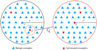
In the process of adversarial example generation, the attacker crafts a perturbation for a benign example such that the resulting example is adversarial. During the generation of adversarial examples, attackers often neglect robustness due to the pursuit of other attributes, such as minimal perturbation, invisibility, target label classification and query efficiency. These attributes and robustness are often incompatible, and thus difficult to achieve simultaneously. Consequently, adversarial examples with small distortion are very close to the decision boundary (wang2019adversarial, ) and most examples in the -neighbourhood of the adversarial example are benign (with respect to the original example ). This is illustrated in Figure 1 (right-part), which is the zoom in of the -neighbourhood of the adversarial example in Figure 1 (left-part).
The above observation can be quantified using robustness. We conduct a quantitative robustness comparison of benign and adversarial examples using the CLEVER score on MNIST and CIFAR10 datasets. For each dataset, we choose the first 100 images from the test dataset as subjects. Adversarial examples are generated by applying four representative attacks: FGSM, BIM, JSMA, and C&W. All the models and attack tools are taken from (feinman2017detecting, ; LID, ), where the parameters are presented in Table 5 in the supplementary material. The CLEVER scores, in the form of a confidence interval of 90% significance level (dekking2005modern, ), are shown in Table 1. Column Label for CLEVER shows the label type for computing the CLEVER scores, where Target-2/5 denotes the top-2/5 label of the example, and LLC (least likely class) is the label with the smallest probability. Column Benign examples shows the CLEVER scores of the benign examples. Columns FGSM, BIM, JSMA and C&W show the CLEVER scores of the adversarial examples generated by FGSM, BIM, JSMA and C&W, respectively. Columns show the ratio of the CLEVER scores of benign examples to that of the adversarial ones for each attack. The last column Avg. shows the ratio of the CLEVER scores of benign examples to that of all the adversarial examples.
| Dataset | Label for | Benign examples | Adversarial examples | Avg. | |||||||
|---|---|---|---|---|---|---|---|---|---|---|---|
| CLEVER | FGSM | BIM | JSMA | C&W | |||||||
| MNIST | Untarget | 3.5572 0.3342 | 0.1093 0.0506 | 32.55 | 0.0256 0.0031 | 138.95 | 0.0550 0.0060 | 64.68 | 0.0004 0.0001 | 8893 | 74.77 |
| Target-2 | 3.6711 0.3296 | 0.1148 0.0427 | 31.98 | 0.0258 0.0031 | 142.29 | 0.0558 0.0063 | 65.79 | 0.0004 0.0001 | 9178 | 74.62 | |
| Target-5 | 3.8303 0.3113 | 0.2047 0.0431 | 18.71 | 0.1582 0.0084 | 24.21 | 0.1898 0.0096 | 20.18 | 0.1384 0.0043 | 27.68 | 22.17 | |
| LLC | 3.8372 0.3097 | 0.2390 0.0421 | 16.06 | 0.1647 0.0071 | 23.30 | 0.2120 0.0076 | 18.10 | 0.1406 0.0045 | 27.29 | 20.29 | |
| CIFAR10 | Untarget | 0.3851 0.1850 | 0.2743 0.1627 | 1.40 | 0.0329 0.0033 | 11.71 | 0.0128 0.0021 | 30.09 | 0.0005 0.0002 | 770 | 4.81 |
| Target-2 | 0.4141 0.1806 | 0.2971 0.1675 | 1.39 | 0.0380 0.0044 | 10.90 | 0.0129 0.0021 | 32.10 | 0.0005 0.0002 | 828 | 4.75 | |
| Target-5 | 0.4657 0.1913 | 0.3389 0.1675 | 1.37 | 0.0971 0.0117 | 4.80 | 0.0610 0.0061 | 7.63 | 0.0925 0.0168 | 5.03 | 3.16 | |
| LLC | 0.4829 0.1913 | 0.3572 0.1713 | 1.35 | 0.1091 0.0132 | 4.43 | 0.0918 0.0095 | 5.26 | 0.1035 0.0180 | 4.67 | 2.92 | |
We can observe that the clever scores of benign examples are much larger than that of adversarial ones for both MNIST and CIFAR10 datasets, though the difference varies from attacks and datasets. This indicates that the difference of robustness between adversarial and benign examples is significant, thus confirms our observation. We also observe that the ratios using untarget/target-2 label for computing the CLEVER scores are larger than the ones using other labels. This is because that the label of untarget or target-2 for each adversarial example is often the label of its benign counterpart, which also confirms our observation that most examples in -neighbourhood of each adversarial example have the same label of the benign counterpart.
3.2. Attack Cost: Adversarial vs. Benign
Based on the above observation, one could design adversarial example detection approaches similar to other characterizations like label change rate (wang2019adversarial, ). However, existing techniques for robustness certification (with statistical guarantees) still have limited scalability, and hence are not able to handle large models efficiently. For instance, on a single GTX 1080 GPU, the cost of computing the CLEVER score is near: 450 seconds for each MNIST example and 1150 seconds for each CIFAR10 example using untarget, 50 seconds for each MNIST example and 128 seconds for each CIFAR10 example using target-2/5.
To effectively and efficiently detect adversarial examples, we propose a novel detection approach, named attack as defense (A2D for short), which uses the cost of attacking an example to test its robustness. The underlying assumption is that the more robust the example is, the more difficult (a larger attack cost) it is to attack. The implication is that we can decide whether an input example is likely to be adversarial by utilizing off-the-shelf attacks.
To leverage attack cost to detect adversarial examples, the first problem needs to be tackled is how to select attacks for defense. In general, the attack cost should be able to be quantified and reflect inputs’ robustness. As a result, FGSM is not suitable since it simply performs one-step perturbation. In contrast, iterative attacks (such as BIM, JSMA, and C&W) that iteratively search for adversarial examples with least distortion could be leveraged, as the costs of such attacks can be quantified and are relevant to inputs’ robustness.
We illustrate this observation using JSMA. JSMA calculates a saliency map based on the Jacobian matrix to model the impact that each pixel imposes on the classification result. During each iteration, JSMA uses a greedy algorithm that modifies certain pixels to increase the probability of the target label. The process is repeated until finding an adversarial example or reaching the termination criteria. The attack cost (time and iteration) of JSMA depends on the robustness of each example. For an example that is less robust than another one , an adversarial example of can be quickly constructed using less time/iteration than the one of . To further test this observation, we compare the attack time of JSMA on 100 MNIST and 100 CIFAR10 examples whose CLEVER scores range from to . The results are reported as scatter plots in Figure 2(a) and Figure 2(b), which confirm our observation.
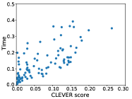
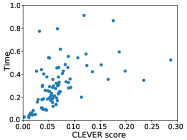
The next problem is then how to characterize attack costs for different kinds of attacks. The most direct indicator of attack costs is the attack time as demonstrated in Figure 2. The attack time of different examples can reflect their robustness. However, the attack time is easily affected by the real-time performance of computing devices in a physical environment, which makes the variance of attack time intolerable. Therefore, in this work, we propose to use the number of iterations of the attacks as the indicator of the attack costs. For an iterative attack, the number of iterations is positively correlated with attack time (cf. the supplementary material).
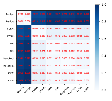
To demonstrate the effectiveness of the attack costs for characterizing adversarial examples, we choose 5 types of images (Benign, FGSM, BIM, DeepFool and C&W), each of which randomly select 1,000 samples, and divided each type of images into two independent sets. Then we use JSMA to attack these images and record the number of iterations required. To show the difference in attack costs, we calculate the average Euclidean distance of the number of iterations between each pair of sets of examples, the results are presented in Figure 3. We can see that for different types of examples (adversarial vs. benign), the distance is enormous. While for the same types of examples (adversarial vs. adversarial or benign vs. benign), the distance is close to zero. It is worth mentioning that for the examples generated by different attacks, the distance is also very similar, meaning that even if the adversarial examples are generated by different attacks, they are also “cognate” examples and have similar attack costs.
Utilizing the diversity of attack methods, an ensemble detection method can be constructed jointly. As we mentioned before, iterative attacks have the potential to be used as defense, so we can integrate multiple iterative attacks to derive a more robust defense. Different attacks have the ability to capture different characterizations. For example, JSMA crafts adversarial examples based on the norm, while BIM is based on the norm, thus they measure the robustness of inputs under different distance metrics. Thanks to various types of attacks, ensemble multiple attacks will make the defense more reliable and difficult to bypass.
4. Detection Approach
In this section, we consider how to detect adversarial examples by leveraging attack costs. In this work, we propose two effective detection approaches that are based on -nearest neighbors (K-NN) and standard score (Z-score), respectively. The former requires both benign and adversarial examples, while the latter requires only benign examples.
Hereafter, we sometimes denote by attackd the attack that is used as defense, i.e., to generate attack costs.
4.1. K-NN based Detection Approach
Assume that we have two disjoint sets: the set of benign examples and the set of adversarial examples.
Single detector. Let us consider the attackd . The attack cost of attacking an example using the attackd is regarded as the fingerprint of . We can generate a set of fingerprints from the examples by utilizing the attackd . For each unknown input and parameter , we first compute the attack cost of the input using the attackd and then identify the -nearest neighbors of from the set . The set is partitioned into two subsets: and . The input is classified as adversarial if , namely, the number of adversarial examples is larger than that of benign ones in K-neighbourhood of the input .
Ensemble detector. The K-NN based detection approach can be easily generalized from one attackd to multiply attacksd , leading to a more robust detector. Under this setting, the fingerprint of an example is a vector of attack costs, , where for every , is the attack cost of the example by utilizing the attackd . Consequently, we can generate a set of fingerprints from the examples by utilizing the attacksd . Similar to the single attack setting, for each unknown input and parameter , we identify the -nearest neighbors of the fingerprint of the input and partition into two subsets: and . The input is classified as adversarial if .
4.2. Z-Score based Detection Approach
Z-score is a well-known concept in statistics for measuring a sample in terms of its relationship to the mean and standard deviation of a dataset (LM11, ). The Z-score of a sample is defined by: , where is the sample mean and is the sample standard deviation. Intuitively, the score indicates how many standard deviations that the sample is far away from the sample mean. Our Z-Score based detection approach leverages the distribution of attack costs of benign examples to check whether an example is adversarial or not. Thus, it is likely more robust with respect to unseen attacks.
Single detector. Let us consider a set of benign examples and an attackd as defense. We can compute the distribution of attack costs of the examples in . Assume that the distribution is an approximately normal distribution . Otherwise, we can transform it by applying the Box-Cox power transformation (boxcox, ). Thus, the Z-score of an example is defined as: , where denotes the cost of attacking using the attackd . For a given ratio of the sample standard deviation as the threshold, based on our observation that adversarial examples are less robust than benign ones, an input is classified to adversarial if , i.e., is standard deviations away from the sample mean.
Ensemble detector. We can also generalize this approach from one attackd to multiply attacksd . For each attackd , we can construct a Z-Score based detector , resulting in detectors . The ensemble detector determines whether an input is adversarial or not by taking into account the results of all the detectors . Consider , the ensemble detector classifies an input to benign if detectors classify the input to benign, otherwise adversarial. The ensemble detector would have high true positive rates when , high true negative rates when .


5. Evaluation
In this section, we evaluate our approach on three widely used datasets MNIST, CIFAR10 and ImageNet. The experiments are designed to answer the following research questions:
-
RQ1.
How to select effective attacks for defense?
-
RQ2.
How effective are the selected attacks for defense?
-
RQ3.
How effective and efficient is A2D (i.e., detection)?
5.1. RQ1: Attack Selection
We answer RQ1 by comparing attack costs of adversarial and benign examples. Adversarial examples are crafted in the same setting as in Section 3.1, using the first 1,000 images from MNIST.
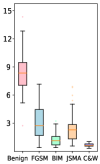
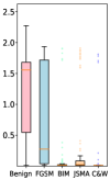
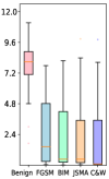
For defense, we choose eight attacks: FGSM, BIM, BIM2 (BIM under norm), JSMA, C&W, L-BFGS, LSA, DBA from Foolbox (RBB17, ), recommended by (TCBM20, ). For ease of reading, an attack used as a defense is marked by a subscript , e.g., FGSMd. According to the results of Table 1, we use untarget attack as defense, unless the attack only supports target attack for which we use target-2 attack. We use the default parameters of Foolbox except that BIMd and BIM2d immediately terminate when an adversarial example is found, and DBAd terminates when the MSE between the adversarial example and its original version is less than 0.02, otherwise the number of iterations is fixed, namely, the attack costs of all the examples will be similar.
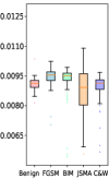
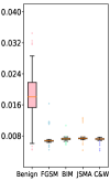
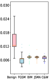
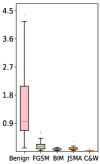
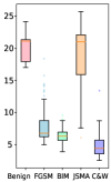
The results in terms of attack time are reported as box plots in Figures 4. It is not surprising that the attack time of adversarial and benign examples using FGMSd are similar, as it is a one-step attack. Though the results show the variation between different attacks and defenses, the differences are often significant when an iterative attack is used as defense, e.g., BIMd, BIM2d, JSMAd, L-BFGSd and DBAd. We find that the differences are not stable when C&Wd and LSAd are used. This is because that C&Wd implements a binary search to minimize distortion and may stop searching when there is a bottleneck, while LSAd suffers from the lower attack success rate which causes it to have many outliers.
Based on the above results, considering the efficiency and discrepancy in attack time between benign and adversarial examples, BIMd, BIM2d, JSMAd, and DBAd will be used as defense in the follow-up experiments. These four methods cover both white-box and black-box attacks, as well as different distance metrics , and . It should be noted that with an amount of adversarial attacks being proposed (more than 2,000 papers in 2020), it is impossible to evaluate all of them. In this work, we only analyze the pros and cons of the above methods and choose suitable attacks.
The above experiments demonstrate how to quickly select a suitable attack as defense. In order to ensure the reliability of BIMd, BIM2d, JSMAd, and DBAd, we also analyze the numbers of iterations. The results are reported as box plots in Figure 5, where the maximal number of iterations of BIMd and BIM2d is increased from the default value 10 to 500 in order to obtain a more significant difference. Remark that we did not tune parameters, these widely used parameters are sufficient to achieve expected results. Fine-tuning parameters may yield better results. We can observe that the differences in the numbers of iterations are consistent with that of attack time, therefore. Since the number of iterations does not depend on computing devices, thus, we will use the number of iterations as the indicator of attack costs in the follow-up experiments.
5.2. RQ2: Effectiveness of Attacks as Defense
We answer RQ2 by comparing our approach with four promising approaches as baselines. The evaluation metric used here is AUROC (area under the receiver operating characteristic curve), which is one of the most important evaluation metrics for measuring the performance of classification indicators. The large the AUROC, the better the approach for detecting adversarial examples.
The first one (feinman2017detecting, ), denoted by BL1, uses a Gaussian Mixture Model to model outputs from the final hidden layer of a CNN, which was considered to be the most effective defense on MNIST among ten detections in (CW17a, ). The second one (LID, ), denoted by BL2, uses local intrinsic dimension to represent and distinguish adversarial subspace and claims to be better than BL1. BL3 (wang2019adversarial, ) uses label change rate through model mutation testing to distinguish adversarial examples. BL4 (Wang2019Dissector, ) dissects the middle layer outputs to construct a fault tolerance approach. We emphasize that BL3 and BL4 (Wang2019Dissector, ) were published in ICSE’19 and ICSE’20, respectively. BL2 is implemented on BL1 which is implemented on Keras (called Env1), while BL3 and BL4 is implemented on Pytorch (called Env2). Since the performance of these four defenses may vary due to platforms, CNN models and attack settings, for a fair comparison, we implement our approach in both Env1 and Env2 and conduct comparison directly using the same target models and attacks provided by each of them. (Parameters are given in Tables 5 and 6 in the supplementary material.)
| Env1 | Attack | JSMAd | BIMd | BIM2d | DBAd | BL1 | BL2 |
| MNIST | FGSM | 0.9653 | 0.9922 | 0.9883 | 0.9504 | 0.8267 | 0.9161 |
| BIM | 0.9986 | 0.9996 | 0.9995 | 0.9625 | 0.9786 | 0.9695 | |
| JSMA | 0.9923 | 0.9922 | 0.9914 | 0.9497 | 0.9855 | 0.9656 | |
| C&W | 1.0 | 1.0 | 1.0 | 0.9672 | 0.9794 | 0.9502 | |
| CIFAR10 | FGSM | 0.6537 | 0.712 | 0.6474 | 0.6977 | 0.7015 | 0.7891 |
| BIM | 0.8558 | 0.8636 | 0.861 | 0.8276 | 0.8255 | 0.8496 | |
| JSMA | 0.9459 | 0.955 | 0.9526 | 0.9452 | 0.8421 | 0.9475 | |
| C&W | 0.9905 | 0.9984 | 0.9988 | 0.9833 | 0.9217 | 0.9799 | |
| Env2 | Attack | JSMAd | BIMd | BIM2d | DBAd | BL3 | BL4 |
| MNIST | FGSM | 0.9665 | 0.9883 | 0.9846 | 0.9595 | 0.9617 | - |
| JSMA | 0.9971 | 0.9984 | 0.9974 | 0.984 | 0.9941 | - | |
| DeepFool | 0.9918 | 0.9971 | 0.9951 | 0.9587 | 0.9817 | - | |
| C&W | 0.9456 | 0.9870 | 0.9769 | 0.8672 | 0.9576 | - | |
| BB | 0.9746 | 0.9895 | 0.9852 | 0.9535 | 0.9677 | - | |
| CIFAR10 | FGSM | 0.8808 | 0.8994 | 0.8998 | 0.8746 | 0.8617 | - |
| JSMA | 0.9774 | 0.9890 | 0.9873 | 0.9566 | 0.9682 | - | |
| DeepFool | 0.9832 | 0.9898 | 0.9902 | 0.9769 | 0.9614 | ||
| C&W | 0.8842 | 0.9176 | 0.9175 | 0.9004 | 0.9063 | - | |
| ImageNet | FGSM | 0.973 | 0.9763 | 0.9782 | 0.9625 | - | 0.9617 |
| JSMA | 0.9962 | 0.9805 | 0.99 | 0.9937 | - | 0.9695 | |
| DeepFool | 0.9958 | 0.9793 | 0.9892 | 0.9891 | - | 0.9924 | |
| C&W | 0.9873 | 0.9731 | 0.9801 | 0.9924 | - | 0.9636 |
Table 2 shows the results in AUROC, where the best one is highlighted in bold font. Note that BL1, BL2 and BL3 only support the MNIST and CIFAR10 datasets, thus there are no results on the ImageNet dataset. Though BL4 considered all these datasets, its open source tool only supports the ImageNet dataset when we conduct experiments. Overall, we can observe that our approach outperforms the baselines in most cases. It is worth mentioning that our defense parameters are the same in both environments, which shows its universality, namely, users do not need to adjust parameters for a specific DL model or platform.
Among the four defenses JSMAd, BIMd, BIM2d and DBAd on MNIST and CIFAR10, BIMd performs better than the others in almost all the cases, while DBAd performs worse than the others in most cases. This is due to that DBAd is a black-box attack which is less powerful than the other white-box attacks. An interesting phenomenon is that the AUROC of JSMAd and DBAd on ImageNet is better than on MNIST and CIFAR10. This is because that for images with large dimension, each perturbation generated by JSMA and DBA is smaller than that of BIM, resulting in a fine-grained attack as well as a fine-grained indicator of examples’ robustness. One may find that BL2 performs better than the others on CIFAR10 adversarial examples crafted by FGSM. This may be because that the performance of the model is too poor as its accuracy is only 80.3% on the testing dataset (cf. Table 5 in the supplementary material). Due to the poor performance of the CIFAR10 model, most attacks of benign examples can be achieved easily, hence the attack costs of adversarial examples generated by FGSM are close to benign examples. This problem could be alleviated by using state-of-the-art models (such as the model in Env2) or improving the robustness of the model (such as adversarial training, cf. Section 6.2.2).
5.3. RQ3: Effectiveness and Efficiency of A2D
We answer RQ3 by applying our K-NN and Z-score based detectors to check benign examples and adversarial examples generated by the attacks from BL3 in Env2. We do not consider other baselines, which only considered the results of AUROC or do not provide cost analysis. In order to avoid overfitting, we selected different data as the training set and the test set.
5.3.1. Effectiveness
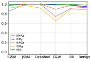
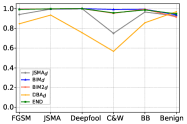
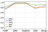
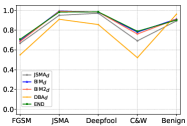
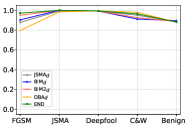
K-NN based detectors. For each dataset, each attackd of BIMd, BIM2d, JSMAd and DBAd as defense and each attack in Env2, we construct a K-NN based detector through the attack costs of 1,000 benign examples and 1,000 attack crafted adversarial examples using the defense attackd. We also construct a K-NN based ensemble detector END, which consists of 1,000 benign examples and 1,000 adversarial examples, where each attack of Env2 contributes 1000 / N adversarial examples (N is the number of attacks). We set . Results on tuning and ratio between benign, adversarial examples and classification algorithms are given in Section C in the supplementary material.
The results are shown in Figures 6(a), 6(c) and 6(e). In general, on average, the accuracies of detectors JSMAd, BIMd, BIM2d, DBAd and END are: 90.84%, 98.09%, 96.17%, 87.42% and 99.36% for MNIST, 86.31%, 87.90%, 87.55%, 85.23% and 92.31% for CIFAR10, 93.44%, 94.08%, 95.08%, 91.64% and 94.48% for ImageNet, We find that DBAd performs worse than others on most cases, which is consistent with AUROC (cf. Table 2). It is worth noting that though the ensemble detector END does not always achieve the best performance, it has the highest average accuracy. Thus, it balances the performances of individual detectors and is more robust.
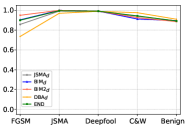
Z-score based detectors. For each dataset, and each attackd of BIMd, BIM2d, JSMAd and DBAd as defense, we construct a Z-score based detector using the normal distribution of attack costs of 1,000 benign examples via attackd, resulting in detectors BIMd, BIM2d, JSMAd and DBAd. The threshold is -1.281552, which yields 10% false positive rate on the 1,000 benign examples. The ensemble detector named by END consists of these four detectors. It classifies an input as benign if no less than 2 detectors classify the input as benign, otherwise adversarial, namely, . Results on tuning and are given in Section C in the supplementary material.
5.3.2. Efficiency
For a fair comparison with BL3, we report the detection costs of the Z-score based detectors here, although it may be slightly worse than K-NN based detector. The reason is that the threshold of Z-score detectors can be easily adjusted to ensure that detection accuracy on benign examples is close to the baseline. As both our method and the baseline BL3 are query-intensive, we compare the number of queries for efficiency comparison.
The results are reported in Table 3. Columns and give the number of queries to the model for adversarial and benign examples on average. Columns Acc and Acc respectively give the accuracy for adversarial and benign examples on average.
By limiting the accuracy on benign examples to the one of BL3, we observe that all the white-box defenses (i.e., JSMAd, BIMd and BIM2d) outperform BL3 in terms of the number of queries on both MNIST and CIFAR10. Furthermore, they also achieve better accuracy than BL3 on CIFAR10, while both BIMd and BIM2d achieve better accuracy than BL3 on MNIST. We also provide the results on ImageNet in Table 3. The results show that on ImageNet, A2D can still detect adversarial examples effectively and efficiently. BIMd/BIM2d are able to detect adversarial examples using one query. This demonstrates that our method is also efficient on high-resolution images. We finally remark that BL3 does not support ImageNet and the other baselines either provide only AUROC without constructing a detector or do not provide cost analysis.
It is not surprising that the cost of DBAd is the largest one, as it is a label-only black-box attack. It is important to mention that black-box attacks used as defense do not need any information of the models, hence using black-box attacks as defense preserve the privacy of the models while its effectiveness is still acceptable.
We emphasize that there is still space for optimization. One latent optimization is to add an upper bound on the number of iterations, as adversarial examples often need fewer iterations than benign. If the number of iterations reaches the bound and the attack fails, the input can be considered as benign. This optimization can reduce the number of iterations (hence queries) for benign examples and both true and false positive rates will not be affected.
| Dataset | Detector | Acc | Threshold | Acc | ||
| MNIST | BL3 | 66 | 96.4% | 463 | - | 89.7% |
| JSMAd | 20 | 95.4% | 240 | 53 | 89.7% | |
| BIMd | 16 | 99.8% | 148 | 122 | ||
| BIM2d | 38 | 99.6% | 352 | 189 | ||
| DBAd | 92 | 88.2% | 319 | 195 | ||
| CIFAR10 | BL3 | 67 | 90.6% | 376 | - | 74.0% |
| JSMAd | 6 | 92.6% | 33 | 13 | 74.0% | |
| BIMd | 14 | 93.0% | 65 | 35 | ||
| BIM2d | 29 | 92.7% | 129 | 71 | ||
| DBAd | 252 | 87.7% | 744 | 409 | ||
| ImageNet | BL3 | - | - | - | - | - |
| JSMAd | 6 | 95.4% | 67 | 11 | 88.6% | |
| BIMd | 1 | 95.2% | 4 | 2 | 89.6% | |
| BIM2d | 1 | 96.7% | 7 | 2 | 88.5% | |
| DBAd | 143 | 93.9% | 451 | 219 | 88.0% |
Discussion. Here we briefly discuss how our approach can be used in practice as different detectors have different accuracies. Considering the tradeoff between the efficiency and accuracy, one can use JSMAd, BIMd or BIM2d as defense according to the dimension of images. If one expects a more reliable and higher accurate detector, an ensemble detector such as the END detector can be used. If the privacy of the model matters, a black-box attack based detector such as DBAd is better.
5.4. Threats to Validity
The threats to validity of our study include external and internal threats. The selection of the subject datasets and target models could be one of the external threats. We tried to counter this issue by using 3 widely-used datasets and 5 pre-trained models from well-established works.
The second external threat is the works we chose for comparison. To mitigate this threat, we compare with the works from both the artificial intelligence community (e.g., BL1 and BL2) and the software engineering community (e.g., BL3 and BL4). BL1 is the most effective defense on MNIST among ten detections in (CW17a, ), while BL2 is claimed better than BL1 (LID, ). Both BL1 and BL2 are widely-used for comparison in the literature (shan2020gotta, ; ma2019nic, ; HeWCCS17, ; lee2018simple, ). BL3 and BL4 are state-of-the-art methods from the perspective of software engineering. It is worth noting that the comparison of baselines was conducted on the repositories and parameters provided by the original authors, to reproduce their best performance, although it may be unfair to our method.
A further external threat is the knowledge of the adversary. The same to baselines, we evaluated our approach against the original models and assume that the adversary is unaware of the existence of the detection. In practice, the adversary may learn that A2D has been used via social engineering or other methods, and use a more threatening, specified attack method, called adaptive attacks in (TCBM20, ). We discuss and evaluate adaptive attacks against our defense method in Section 6. We do not perform the same adaptive attack on the baselines, as adaptive attacks are usually designed for each specific defense method.
The internal threat mainly comes from the selection of attacks as defense. We approximate model robustness of examples by the cost of attacking them while attacks may differ in their capability. To mitigate this threat, we studied various attacks, covering white-box and black-box attacks, and , and norm based attacks. Experimental results indicate that our defense performs well regardless of the selected attacks, although a minor difference can be observed. Based on this, we conclude that our answers to research questions should generally hold.
6. On Adaptive Attacks
Lots of effective defenses have been shown to be ineffective in the presence of adaptive attacks (CW, ; CW17a, ; carlini2017magnet, ; HeWCCS17, ; TCBM20, ). Thus, adaptive attacks are the main threat to defense approaches. In this section, we study possible adaptive attacks to our defense.
6.1. Potential Bypass Approaches
6.1.1. Increasing Attack Costs
A straightforward approach that may be used to bypass our defense is to increase the attack costs so that the attack costs of adversarial and benign examples are similar. To increase attack costs of adversarial examples, one can incorporate attack costs into the loss function used to identify adversarial examples. For instance, the adversary could change the loss function to
where is the original loss function, is a parameter for balancing two terms of , is the expected attack cost such as the mean of attack costs of benign examples or even the threshold of our Z-score based detection approach, and denotes the attack cost of via some attacks. Minimizing the new loss increases the attack cost until exceeding .
Discussion. This adaptive attack to our defense is infeasible if not impossible. First, the function non-differentiable, consequently, the loss function cannot be solved via gradient-based algorithms. Second, non-gradient-based iterative attacks have to run some attacks internally during each iteration in order to check if the attack succeeds or not. This definitely results in high computational complexity, thus becoming infeasible .
6.1.2. Increasing Robustness
An alternative approach that may be used to bypass our defense is to increase the robustness of adversarial examples, aiming to indirectly increase the attack costs. However, it is non-trivial to directly control the robustness of adversarial examples. We propose to increase the confidence/strength of adversarial examples, initially considered by Carlini and Wagner (CW, ) for increasing transferability of adversarial examples between different models. Confidence is controlled by introducing a parameter into the loss function , thus, the loss function becomes
where the larger the parameter , the higher the confidence of the adversarial example.
The relation between robustness and confidence of adversarial examples is confirmed by the following experiment. We mount the C&W attack on the previous 100 MNIST and 100 CIFAR10 images under the same setting as (carlini2017magnet, ), by varying the value of and measuring the robustness using the CLEVER scores. The results are reported in Table 4. The experiment results show that the adversary is able to increase the robustness of adversarial examples by increasing the confidence. Therefore, high-confidence adversarial examples have the potential to bypass our defense.
| 0 | 2 | 4 | 6 | 8 | ||
|---|---|---|---|---|---|---|
| MNIST | CLEVER Score | 0.11 | 0.14 | 0.14 | 0.17 | |
| No. of Iterations | 1.01 | 10.36 | 20.28 | 31.29 | 42.59 | |
| distance | 1.71 | 1.91 | 2.11 | 2.32 | 2.53 | |
| CIFAR10 | CLEVER Score | 0.07 | 0.08 | 0.09 | 0.13 | |
| No. of Iterations | 1.37 | 8.53 | 17.29 | 24.47 | 34.4 | |
| distance | 0.41 | 0.52 | 0.67 | 0.82 | 0.99 | |
Discussion. This adaptive attack is feasible, but will introduce large distortion into adversarial examples when increases, observed from Table 4. As our defense changes neither inputs nor models, it can be seamlessly combined with other defenses to defend against this adaptive attack.
- •
-
•
The second method is to combine with adversarial training (Intriguing, ; FGSM15, ; MyMSTV17, ) which enhances the DL model. Indeed, a successful attack to an adversarially trained model often introduces large distortion while the adaptive attack also introduces large distortion to bypass our defense, consequently, the distortion becomes too large to be human-perceptible.
6.2. Evaluation of Adaptive Attacks
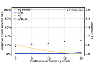
Since the first adaptive attack is infeasible, we only evaluate the second one which is implemented based on C&W (carlini2017magnet, ). We evaluate this adaptive attack by varying the parameter from 0 to 20.
To evaluate the effectiveness of our defense combined with other defenses, we consider the autoencoder based detector (AE for short) (MC17, ) and PGD adversarial training (AT for short) (MyMSTV17, ). The AE trains a classifier based on benign examples in order to detect any adversarial examples with large distortion by checking if is greater than a different threshold , where is a distance function, e.g., the mean squared error .
6.2.1. A2D with AE
For ease of evaluation, we conduct experiments using the MNIST dataset under the same settings as (MC17, ) which provides a trained AE. In our experiments, the maximal norm distortion is 8.4 which is approximated from the maximal norm distortion 0.3 in Madry’s challenges (mnistchallenge19, ). Note that our maximal distortion allows perturbations to be greater than the maximal distortion for some pixels. Such large perturbations are often challenging for defense. We use BIMd as defense and the corresponding Z-score based detector which only requires benign examples. Thus, it is a relatively weaker defense. We denote by A2D our detector and A2D + AE the combined detector.
Results. The results are reported in Figure 7(a). From Figure 7(a) , we can observe that without any defense, the attack success rate (ASR) is always 100%. With the increase of , the detection rate of our defense A2D decreases slightly. Specifically, A2D is able to detect all of the adversarial examples when , while only about 3% of adversarial examples can bypass A2D when . We also observe that both the distortion and detection rate of AE increase with the increase of . About 21% of adversarial examples can bypass AE when , while all adversarial examples can be detected by AE when . Therefore, the ASR is always 0% when the combined defense A2D + AE is applied.
Summary. The above results demonstrate the benefit of combining two complementary defenses. Although an adaptive attack can slightly reduce the effectiveness of A2D by increasing robustness of adversarial examples, the combination of A2D and AE is able to completely defend against such adaptive attack.
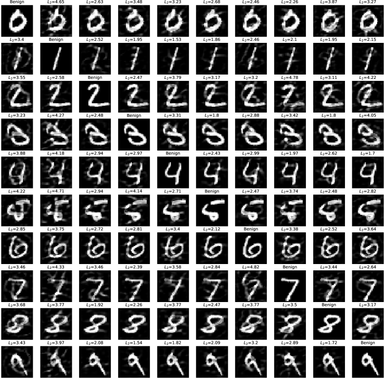
Case study. Figure 8 shows adversarial examples of a target attack from 4 to 0 with different . The perturbation for is about twice larger than that for and can be easily detected by AE. More images are given in Section D in the supplementary material.

6.2.2. A2D with AT
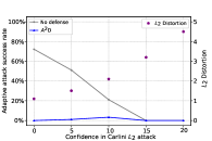
For ease of evaluation, we conduct experiments using the CIFAR10 dataset under the same settings as (MyMSTV17, ) which provides an adversarially trained DL model. In our experiments, the maximal norm distortion is 1.6 which is approximated from the maximal norm distortion 0.03 in Madry’s challenges (mnistchallenge19, ). We use the same Z-score based detector as in Section 6.2.1.
Results. The results are shown in Figure 7(b). Note that adversarial training (AT) is not a detector, so ‘No defense’ is equivalent to ‘AT’. We can observe that AT is not very promising when is smaller, e.g., 72% ASR for . With the increase of (i.e., increasing robustness of adversarial examples), the ASR drops to 21% when and 0% ASR when . This is because that finding adversarial examples with distortion limited to the maximal threshold becomes more difficult for the adversarially trained model. Recall that our defense A2D is good at detecting adversarial examples with small distortion (i.e., low-confidence). Therefore, the combined defense is very effective. For instance, all adversarial examples with can be detected by A2D, hence the ASR drops from 72% to 0%. The adaptive attack achieves no more than 3% ASR on the adversarially trained model.
Summary. To bypass our defense on adversarially trained models, the adversary has to introduce much large distortion. When perturbations are limited to human-imperceptible, it becomes difficult to bypass our defense on adversarially trained models.
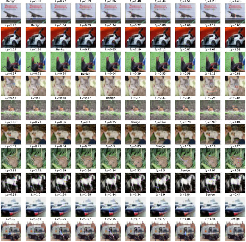
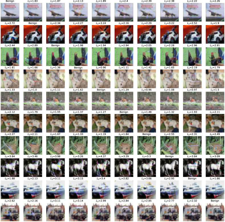
Case study. Figure 9 shows adversarial examples of a target attack from ‘airplane’ to ‘cat’. Without any defense, an adversarial example with less distortion can be crafted, cf. Figure 9(b). With AT, it requires more distortion to craft an adversarial example, cf. Figure 9(c). If both A2D and AT are enabled, it requires much more distortion to craft adversarial examples, cf. Figure 9(d). Now the distortion is too large to be human-perceptible, and we can clearly see the silhouettes of ‘cats’ on the adversarial example. More images are given in Section D in the supplementary material.


7. Related Work
As a new type of software system, neural networks have received extensive attention over the last five years. We classify existing works along three dimensions: adversarial attack, adversarial defense, and neural network testing & verification.
Adversarial attack. Adversarial attacks aim to misjudge the neural network by adding perturbations that are imperceptible to humans. We have introduced common attacks in Section 2. We selected multiple types of methods to generate adversarial examples, FGSM (FGSM15, ), BIM (KGB17, ), JSMA (JSMA, ), DeepFool (DeepFool, ), C&W (CW, ) and substitute model attack (PMG16, ). We also selected multiple attacks as defense. Meanwhile, several adversarial examples have the ability to carry out attacks in the real environment (KGB17, ; EEF0RXPKS18, ; JMLHW19, ), and pose threats to neural networks, which is a new programming paradigm.
Adversarial defense. A typical defense method is adversarial training (Intriguing, ; FGSM15, ; KGB17, ; MyMSTV17, ), which produces adversarial examples and injects them into training data. Another type of defenses protects models by pre-processing the input data (buckman2018thermometer, ; guo2017countering, ; xie2017mitigating, ) or projects potential adversarial examples onto the benign data manifold before classifying them (song2017pixeldefend, ; MC17, ). Detection is another defense approach to adversarial examples. If an input is detected as adversarial, it will be rejected without being fed to the model (feinman2017detecting, ; lee2018simple, ; LID, ; Xu0Q18, ). However, it has been shown that most defense methods except adversarial training can be easily bypassed by adaptive attack with backward pass differentiable approximation and expectation over transformation (athalye2018obfuscated, ; AEIK18, ; TCBM20, ; CW17a, ). Until today this problem is still of considerable interest. However, most detection methods are not effective on high-resolution images (e.g., ImageNet dataset) (wang2019adversarial, ; MC17, ; LID, ; feinman2017detecting, ) or do not consider adaptive attacks (wang2019adversarial, ; MC17, ; LID, ; feinman2017detecting, ; wang2019adversarial, ). Our defense method is effective on 3 widely-used datasets covering both low- and high-resolution images. We also evaluated our defense against potential adaptive attacks and demonstrate its effectiveness.
Neural network testing & verification. Some works look for vulnerabilities in neural networks from the perspective of software testing. For example, DeepXplore (PCYJ17, ) proposed a testing technique to find adversarial examples guided neuron coverage. After that, a series of coverage criteria have been proposed for neural network testing (SHK18, ; MJZSXLCSLLZW18, ; kim2019guiding, ). Other testing methods also have been adapted to test neural networks such as concolic testing (SWRHKK18, ), mutation testing (MZSXLJXLLZW18, ; shen2018munn, ), and so on (WHK18, ; MaJXLLLZ19, ). Some testing methods focus on different application scenarios of neural networks, including DeepTest (TPJR18, ), DeepRoad (zhang2018deeproad, ), Deepbillboard (zhou2020deepbillboard, ) and object-relevance metamorphic testing (tian2019testing, ). Some other works focus on testing the neural network at the architecture level (zhang2020detecting, ) or the deep learning library itself (wang2020deep, ). We do not use testing criteria to model the robustness of examples, as testing criteria are not necessarily correlated with robustness (yan2020correlations, ; dongempirical, ).
Various formal verification techniques have been proposed to verify robustness property against neural networks (HKWW17, ; GKPB18, ; PT10, ; KBDJK17, ; wang2018efficient, ; BILVNC16, ; DSGMK18, ; TXT18, ; EGK20, ; SGPV19, ; SGMPV18, ; WZCSHDBD18, ; Ehl17, ; GMDTCV18, ). Formal verification provides provable or theoretic guarantees, and robustness is also the source of our defense approach. However, formal verification suffers from the scalability problem, due to the high computational complexity. Therefore, we used attack cost instead.
(wang2019adversarial, ) and (Wang2019Dissector, ) are very close to our defense approach. They also considered the problem of identifying adversarial examples from the perspective of software engineering, by leveraging mutation testing and model anatomy respectively. However, both of them have to modify the original model, while our defense approach does not, hence is easy to deploy. When using white-box attacks as defense, the model only needs to provide an interface for logits and gradients, rather than model parameters. When using black-box attacks as defense, the model only needs to provide the classification results, thus protecting the privacy of the model. Inspired by (carlini2017magnet, ; HeWCCS17, ; TCBM20, ; ma2019nic, ), we discussed and evaluated adaptive attacks to our defense. However, (wang2019adversarial, ) and (Wang2019Dissector, ) do not consider adaptive attacks, hence it is unclear whether they are still effective under adaptive attacks.
8. Conclusion
We have proposed a novel characterization of adversarial examples via robustness. Based on the characterization, we proposed a novel detection approach, named attack as defense (A2D), which utilizes existing attacks to measure examples’ robustness. We conducted extensive experiments to evaluate our observations and detection approach A2D, showing that it outperforms four recent promising approaches. We also thoroughly discussed the main threat (i.e., adaptive attacks) to our defense and evaluated them to our defense. By combing our defense with an existing defense and adversarial training, the results are very promising, e.g., the ASR drops from 72% to 0% on CIFAR10, and drops from 100% to 0% on MNIST.
References
- (1) Apollo. An open, reliable and secure software platform for autonomous driving systems. http://apollo.auto, 2018.
- (2) Anish Athalye, Nicholas Carlini, and David A. Wagner. Obfuscated gradients give a false sense of security: Circumventing defenses to adversarial examples. In Proceedings of the 35th International Conference on Machine Learning, pages 274–283, 2018.
- (3) Anish Athalye, Logan Engstrom, Andrew Ilyas, and Kevin Kwok. Synthesizing robust adversarial examples. In Proceedings of the 35th International Conference on Machine Learning, pages 284–293, 2018.
- (4) Osbert Bastani, Yani Ioannou, Leonidas Lampropoulos, Dimitrios Vytiniotis, Aditya V. Nori, and Antonio Criminisi. Measuring neural net robustness with constraints. In NIPS, pages 2613–2621, 2016.
- (5) George EP Box and David R Cox. An analysis of transformations. Journal of the Royal Statistical Society: Series B (Methodological), 26(2):211–243, 1964.
- (6) Wieland Brendel, Jonas Rauber, and Matthias Bethge. Decision-based adversarial attacks: Reliable attacks against black-box machine learning models. In International Conference on Learning Representations, 2018.
- (7) Jacob Buckman, Aurko Roy, Colin Raffel, and Ian Goodfellow. Thermometer encoding: One hot way to resist adversarial examples. In International Conference on Learning Representations, 2018.
- (8) Nicholas Carlini and David Wagner. Magnet and “efficient defenses against adversarial attacks” are not robust to adversarial examples. CoRR, abs/1711.08478, 2017.
- (9) Nicholas Carlini and David A. Wagner. Adversarial examples are not easily detected: Bypassing ten detection methods. In Proceedings of the 10th ACM Workshop on Artificial Intelligence and Security, pages 3–14, 2017.
- (10) Nicholas Carlini and David A. Wagner. Towards evaluating the robustness of neural networks. In Proceedings of IEEE Symposium on Security and Privacy (S&P), pages 39–57, 2017.
- (11) Pin-Yu Chen, Yash Sharma, Huan Zhang, Jinfeng Yi, and Cho-Jui Hsieh. EAD: elastic-net attacks to deep neural networks via adversarial examples. In Proceedings of the Thirty-Second AAAI Conference on Artificial Intelligence (AAAI), pages 10–17, 2018.
- (12) Frederik Michel Dekking, Cornelis Kraaikamp, Hendrik Paul Lopuhaä, and Ludolf Erwin Meester. A Modern Introduction to Probability and Statistics: Understanding why and how. Springer Science & Business Media, 2005.
- (13) Yizhen Dong, Peixin Zhang, Jingyi Wang, Shuang Liu, Jun Sun, Jianye Hao, Xinyu Wang, Li Wang, Jinsong Dong, and Ting Dai. An empirical study on correlation between coverage and robustness for deep neural networks.
- (14) Yuchao Duan, Zhe Zhao, Lei Bu, and Fu Song. Things you may not know about adversarial example: A black-box adversarial image attack. CoRR, abs/1905.07672, 2019.
- (15) Krishnamurthy Dvijotham, Robert Stanforth, Sven Gowal, Timothy A. Mann, and Pushmeet Kohli. A dual approach to scalable verification of deep networks. CoRR, abs/1803.06567, 2018.
- (16) Rüdiger Ehlers. Formal verification of piece-wise linear feed-forward neural networks. In Proceedings of the 15th International Symposium on Automated Technology for Verification and Analysis, pages 269–286, 2017.
- (17) Yizhak Yisrael Elboher, Justin Gottschlich, and Guy Katz. An abstraction-based framework for neural network verification. In Proceedings of The 32nd International Conference on Computer-Aided Verification (CAV), 2020.
- (18) Kevin Eykholt, Ivan Evtimov, Earlence Fernandes, Bo Li, Amir Rahmati, Chaowei Xiao, Atul Prakash, Tadayoshi Kohno, and Dawn Song. Robust physical-world attacks on deep learning visual classification. In Proceedings of 2018 IEEE Conference on Computer Vision and Pattern Recognition, pages 1625–1634, 2018.
- (19) Reuben Feinman, Ryan R Curtin, Saurabh Shintre, and Andrew B Gardner. Detecting adversarial samples from artifacts. arXiv preprint arXiv:1703.00410, 2017.
- (20) Timon Gehr, Matthew Mirman, Dana Drachsler-Cohen, Petar Tsankov, Swarat Chaudhuri, and Martin T. Vechev. AI2: safety and robustness certification of neural networks with abstract interpretation. In Proceedings of the 2018 IEEE Symposium on Security and Privacy, pages 3–18, 2018.
- (21) Ian Goodfellow, Jonathon Shlens, and Christian Szegedy. Explaining and harnessing adversarial examples. In Proceedings of the 3th International Conference on Learning Representations (ICLR), 2015.
- (22) Divya Gopinath, Guy Katz, Corina S. Pasareanu, and Clark Barrett. Deepsafe: A data-driven approach for assessing robustness of neural networks. In Proceedings of the 16th International Symposium on Automated Technology for Verification and Analysis, pages 3–19, 2018.
- (23) Chuan Guo, Mayank Rana, Moustapha Cisse, and Laurens Van Der Maaten. Countering adversarial images using input transformations. arXiv preprint arXiv:1711.00117, 2017.
- (24) Warren He, James Wei, Xinyun Chen, Nicholas Carlini, and Dawn Song. Adversarial example defense: Ensembles of weak defenses are not strong. In Proceedings of the 11th USENIX Workshop on Offensive Technologies, 2017.
- (25) Xiaowei Huang, Marta Kwiatkowska, Sen Wang, and Min Wu. Safety verification of deep neural networks. In Proceedings of the 29th International Conference on Computer Aided Verification, pages 3–29, 2017.
- (26) Andrew Ilyas, Logan Engstrom, Anish Athalye, and Jessy Lin. Black-box adversarial attacks with limited queries and information. In Proceedings of the 35th International Conference on Machine Learning, pages 2142–2151, 2018.
- (27) Steve T.K. Jan, Joseph Messou, Yen-Chen Lin, Jia-Bin Huang, and Gang Wang. Connecting the digital and physical world: Improving the robustness of adversarial attacks. In AAAI, 2019.
- (28) Guy Katz, Clark W. Barrett, David L. Dill, Kyle Julian, and Mykel J. Kochenderfer. Reluplex: An efficient SMT solver for verifying deep neural networks. In Proceedings of the 29th International Conference on Computer Aided Verification, pages 97–117, 2017.
- (29) Jinhan Kim, Robert Feldt, and Shin Yoo. Guiding deep learning system testing using surprise adequacy. In 2019 IEEE/ACM 41st International Conference on Software Engineering (ICSE), pages 1039–1049. IEEE, 2019.
- (30) Alex Krizhevsky. Learning multiple layers of features from tiny images. Technical report, 2009.
- (31) Alexey Kurakin, Ian Goodfellow, and Samy Bengio. Adversarial examples in the physical world. In Proceedings of International Conference on Learning Representations, 2017.
- (32) Madry Lab. MNIST and cifar10 adversarial examples challenges. https://github.com/MadryLab, September 2020.
- (33) Richard J. Larsen and Morris L. Marx. An Introduction to Mathematical Statistics and Its Applications. Prentice Hall, 2011.
- (34) Yann LeCun, Corinna Cortes, and Christopher JC Burges. The mnist database of handwritten digits, 1998.
- (35) Kimin Lee, Kibok Lee, Honglak Lee, and Jinwoo Shin. A simple unified framework for detecting out-of-distribution samples and adversarial attacks. In Advances in Neural Information Processing Systems, pages 7167–7177, 2018.
- (36) Jiajun Lu, Theerasit Issaranon, and David A. Forsyth. Safetynet: Detecting and rejecting adversarial examples robustly. In Proceedings of the IEEE International Conference on Computer Vision, pages 446–454, 2017.
- (37) Lei Ma, Felix Juefei-Xu, Minhui Xue, Bo Li, Li Li, Yang Liu, and Jianjun Zhao. Deepct: Tomographic combinatorial testing for deep learning systems. In Xinyu Wang, David Lo, and Emad Shihab, editors, 26th IEEE International Conference on Software Analysis, Evolution and Reengineering, SANER 2019, Hangzhou, China, February 24-27, 2019, pages 614–618. IEEE, 2019.
- (38) Lei Ma, Felix Juefei-Xu, Fuyuan Zhang, Jiyuan Sun, Minhui Xue, Bo Li, Chunyang Chen, Ting Su, Li Li, Yang Liu, Jianjun Zhao, and Yadong Wang. Deepgauge: multi-granularity testing criteria for deep learning systems. In Proceedings of the 33rd ACM/IEEE International Conference on Automated Software Engineering, pages 120–131, 2018.
- (39) Lei Ma, Fuyuan Zhang, Jiyuan Sun, Minhui Xue, Bo Li, Felix Juefei-Xu, Chao Xie, Li Li, Yang Liu, Jianjun Zhao, and Yadong Wang. Deepmutation: Mutation testing of deep learning systems. In 29th IEEE International Symposium on Software Reliability Engineering, pages 100–111, 2018.
- (40) Shiqing Ma, Yingqi Liu, Guanhong Tao, Wen-Chuan Lee, and Xiangyu Zhang. NIC: detecting adversarial samples with neural network invariant checking. In 26th Annual Network and Distributed System Security Symposium, NDSS 2019, San Diego, California, USA, February 24-27, 2019, 2019.
- (41) Xingjun Ma, Bo Li, Yisen Wang, Sarah M. Erfani, Sudanthi N. R. Wijewickrema, Grant Schoenebeck, Dawn Song, Michael E. Houle, and James Bailey. Characterizing adversarial subspaces using local intrinsic dimensionality. In Proceedings of the 6th International Conference on Learning Representations, 2018.
- (42) Aleksander Madry, Aleksandar Makelov, Ludwig Schmidt, Dimitris Tsipras, and Adrian Vladu. Towards deep learning models resistant to adversarial attacks. In Proceedings of International Conference on Learning Representations, 2018.
- (43) Dongyu Meng and Hao Chen. Magnet: A two-pronged defense against adversarial examples. In Proceedings of the 2017 ACM SIGSAC Conference on Computer and Communications Security, pages 135–147, 2017.
- (44) Seyed-Mohsen Moosavi-Dezfooli, Alhussein Fawzi, Omar Fawzi, and Pascal Frossard. Universal adversarial perturbations. In Proceedings of 2017 IEEE Conference on Computer Vision and Pattern Recognition, pages 86–94, 2017.
- (45) Seyed-Mohsen Moosavi-Dezfooli, Alhussein Fawzi, and Pascal Frossard. Deepfool: A simple and accurate method to fool deep neural networks. In Proceedings of 2016 IEEE Conference on Computer Vision and Pattern Recognition, pages 2574–2582, 2016.
- (46) Nina Narodytska and Shiva Prasad Kasiviswanathan. Simple black-box adversarial attacks on deep neural networks. In 2017 IEEE Conference on Computer Vision and Pattern Recognition Workshops, pages 1310–1318, 2017.
- (47) Anh Mai Nguyen, Jason Yosinski, and Jeff Clune. Deep neural networks are easily fooled: High confidence predictions for unrecognizable images. In Proceedings of 2015 IEEE Conference on Computer Vision and Pattern Recognition, pages 427–436, 2015.
- (48) Nicolas Papernot, Patrick D. McDaniel, and Ian J. Goodfellow. Transferability in machine learning: from phenomena to black-box attacks using adversarial samples. CoRR, abs/1605.07277, 2016.
- (49) Nicolas Papernot, Patrick D. McDaniel, Ian J. Goodfellow, Somesh Jha, Z. Berkay Celik, and Ananthram Swami. Practical black-box attacks against machine learning. In Proceedings of the 2017 ACM on Asia Conference on Computer and Communications Security, pages 506–519, 2017.
- (50) Nicolas Papernot, Patrick D. McDaniel, Somesh Jha, Matt Fredrikson, Z. Berkay Celik, and Ananthram Swami. The limitations of deep learning in adversarial settings. In Proceedings of IEEE European Symposium on Security and Privacy (EuroS&P), pages 372–387, 2016.
- (51) Nicolas Papernot, Patrick D. McDaniel, Xi Wu, Somesh Jha, and Ananthram Swami. Distillation as a defense to adversarial perturbations against deep neural networks. In IEEE Symposium on Security and Privacy, pages 582–597, 2016.
- (52) Kexin Pei, Yinzhi Cao, Junfeng Yang, and Suman Jana. Deepxplore: Automated whitebox testing of deep learning systems. In Proceedings of the 26th Symposium on Operating Systems Principles, pages 1–18, 2017.
- (53) Luca Pulina and Armando Tacchella. An abstraction-refinement approach to verification of artificial neural networks. In Proceedings of the 22nd International Conference on Computer Aided Verification (CAV), pages 243–257, 2010.
- (54) Jonas Rauber, Wieland Brendel, and Matthias Bethge. Foolbox: A python toolbox to benchmark the robustness of machine learning models. arXiv preprint arXiv:1707.04131, 2017.
- (55) Kevin Roth, Yannic Kilcher, and Thomas Hofmann. The odds are odd: A statistical test for detecting adversarial examples. In Proceedings of the 36th International Conference on Machine Learning, pages 5498–5507, 2019.
- (56) Wenjie Ruan, Xiaowei Huang, and Marta Kwiatkowska. Reachability analysis of deep neural networks with provable guarantees. In Proceedings of the Twenty-Seventh International Joint Conference on Artificial Intelligence, pages 2651–2659, 2018.
- (57) Ali Shafahi, Mahyar Najibi, Amin Ghiasi, Zheng Xu, John P. Dickerson, Christoph Studer, Larry S. Davis, Gavin Taylor, and Tom Goldstein. Adversarial training for free! In Proceedings of the 32nd Annual Conference on Neural Information Processing Systems, pages 3353–3364, 2019.
- (58) Shawn Shan, Emily Wenger, Bolun Wang, Bo Li, Haitao Zheng, and Ben Y Zhao. Gotta catch’em all: Using honeypots to catch adversarial attacks on neural networks. In Proceedings of the 2020 ACM SIGSAC Conference on Computer and Communications Security, pages 67–83, 2020.
- (59) Dinggang Shen, Guorong Wu, , and Heung-Il Suk. Deep learning in medical image analysis. Annual Review of Biomedical Engineering, 19:221–248, 2017.
- (60) Weijun Shen, Jun Wan, and Zhenyu Chen. Munn: Mutation analysis of neural networks. In 2018 IEEE International Conference on Software Quality, Reliability and Security Companion (QRS-C), pages 108–115. IEEE, 2018.
- (61) Gagandeep Singh, Timon Gehr, Matthew Mirman, Markus Püschel, and Martin T. Vechev. Fast and effective robustness certification. In Proceedings of the Annual Conference on Neural Information Processing Systems (NeurIPS), pages 10825–10836, 2018.
- (62) Gagandeep Singh, Timon Gehr, Markus Püschel, and Martin T. Vechev. An abstract domain for certifying neural networks. Proc. ACM Program. Lang., 3(POPL):41:1–41:30, 2019.
- (63) Wei Song, Heng Yin, Chang Liu, and Dawn Song. Deepmem: Learning graph neural network models for fast and robust memory forensic analysis. In Proceedings of the 2018 ACM SIGSAC Conference on Computer and Communications Security, pages 606–618, 2018.
- (64) Yang Song, Taesup Kim, Sebastian Nowozin, Stefano Ermon, and Nate Kushman. Pixeldefend: Leveraging generative models to understand and defend against adversarial examples. arXiv preprint arXiv:1710.10766, 2017.
- (65) Youcheng Sun, Xiaowei Huang, and Daniel Kroening. Testing deep neural networks. CoRR, abs/1803.04792, 2018.
- (66) Youcheng Sun, Min Wu, Wenjie Ruan, Xiaowei Huang, Marta Kwiatkowska, and Daniel Kroening. Concolic testing for deep neural networks. In Proceedings of the 33rd ACM/IEEE International Conference on Automated Software Engineerin, pages 109–119, 2018.
- (67) Christian Szegedy, Wojciech Zaremba, Ilya Sutskever, Joan Bruna, Dumitru Erhan, Ian Goodfellow, and Rob Fergus. Intriguing properties of neural networks. In Proceedings of the 2nd International Conference on Learning Representations (ICLR), 2014.
- (68) Yongqiang Tian, Shiqing Ma, Ming Wen, Yepang Liu, Shing-Chi Cheung, and Xiangyu Zhang. Testing deep learning models for image analysis using object-relevant metamorphic relations. arXiv preprint arXiv:1909.03824, 2019.
- (69) Yuchi Tian, Kexin Pei, Suman Jana, and Baishakhi Ray. Deeptest: automated testing of deep-neural-network-driven autonomous cars. In Proceedings of the 40th International Conference on Software Engineering, pages 303–314, 2018.
- (70) Vincent Tjeng, Kai Xiao, and Russ Tedrake. Evaluating robustness of neural networks with mixed integer programming. 2019.
- (71) Florian Tramèr, Nicholas Carlini, Wieland Brendel, and Aleksander Madry. On adaptive attacks to adversarial example defenses. CoRR, abs/2002.08347, 2020.
- (72) Chun-Chen Tu, Pai-Shun Ting, Pin-Yu Chen, Sijia Liu, Huan Zhang, Jinfeng Yi, Cho-Jui Hsieh, and Shin-Ming Cheng. Autozoom: Autoencoder-based zeroth order optimization method for attacking black-box neural networks. In Proceedings of the 33rd AAAI Conference on Artificial Intelligence, pages 742–749, 2019.
- (73) Huiyan Wang, Jingwei Xu, Chang Xu, Xiaoxing Ma, and Jian Lu. Dissector: Input validation for deep learning applications by crossing-layer dissection. In The 42th International Conference on Software Engineering, 2020.
- (74) Jingyi Wang, Guoliang Dong, Jun Sun, Xinyu Wang, and Peixin Zhang. Adversarial sample detection for deep neural network through model mutation testing. In Proceedings of the 41st International Conference on Software Engineering, pages 1245–1256. IEEE Press, 2019.
- (75) Shiqi Wang, Kexin Pei, Justin Whitehouse, Junfeng Yang, and Suman Jana. Efficient formal safety analysis of neural networks. In Proceedings of Annual Conference on Neural Information Processing Systems (NeurIPS), pages 6367–6377, 2018.
- (76) Shiqi Wang, Kexin Pei, Justin Whitehouse, Junfeng Yang, and Suman Jana. Formal security analysis of neural networks using symbolic intervals. In Proceedings of the 27th USENIX Security Symposium on Security, pages 1599–1614, 2018.
- (77) Zan Wang, Ming Yan, Junjie Chen, Shuang Liu, and Dongdi Zhang. Deep learning library testing via effective model generation. In Proceedings of the 28th ACM Joint Meeting on European Software Engineering Conference and Symposium on the Foundations of Software Engineering, pages 788–799, 2020.
- (78) Tsui-Wei Weng, Huan Zhang, Hongge Chen, Zhao Song, Cho-Jui Hsieh, Luca Daniel, Duane S. Boning, and Inderjit S. Dhillon. Towards fast computation of certified robustness for relu networks. In Proceedings of the 35th International Conference on Machine Learning, pages 5273–5282, 2018.
- (79) Tsui-Wei Weng, Huan Zhang, Pin-Yu Chen, Jinfeng Yi, Dong Su, Yupeng Gao, Cho-Jui Hsieh, and Luca Daniel. Evaluating the robustness of neural networks: An extreme value theory approach. In Proceedings of the 6th International Conference on Learning Representations (ICLR), 2018.
- (80) Matthew Wicker, Xiaowei Huang, and Marta Kwiatkowska. Feature-guided black-box safety testing of deep neural networks. In Proceedings of the 24th International Conference on Tools and Algorithms for the Construction and Analysis of Systems, pages 408–426, 2018.
- (81) Cihang Xie, Jianyu Wang, Zhishuai Zhang, Zhou Ren, and Alan Yuille. Mitigating adversarial effects through randomization. arXiv preprint arXiv:1711.01991, 2017.
- (82) Weilin Xu, David Evans, and Yanjun Qi. Feature squeezing: Detecting adversarial examples in deep neural networks. In Proceedings of the 25th Annual Network and Distributed System Security Symposium, 2018.
- (83) Shenao Yan, Guanhong Tao, Xuwei Liu, Juan Zhai, Shiqing Ma, Lei Xu, and Xiangyu Zhang. Correlations between deep neural network model coverage criteria and model quality. In Proceedings of the 28th ACM Joint Meeting on European Software Engineering Conference and Symposium on the Foundations of Software Engineering, pages 775–787, 2020.
- (84) Mengshi Zhang, Yuqun Zhang, Lingming Zhang, Cong Liu, and Sarfraz Khurshid. Deeproad: Gan-based metamorphic testing and input validation framework for autonomous driving systems. In 2018 33rd IEEE/ACM International Conference on Automated Software Engineering (ASE), pages 132–142. IEEE, 2018.
- (85) Yuhao Zhang, Luyao Ren, Liqian Chen, Yingfei Xiong, Shing-Chi Cheung, and Tao Xie. Detecting numerical bugs in neural network architectures. In Proceedings of the 28th ACM Joint Meeting on European Software Engineering Conference and Symposium on the Foundations of Software Engineering, pages 826–837, 2020.
- (86) Husheng Zhou, Wei Li, Zelun Kong, Junfeng Guo, Yuqun Zhang, Bei Yu, Lingming Zhang, and Cong Liu. Deepbillboard: Systematic physical-world testing of autonomous driving systems. In 2020 IEEE/ACM 42nd International Conference on Software Engineering (ICSE), pages 347–358. IEEE, 2020.
Appendix A Environments
For reproductivity of this work, all the information of the target models and attack parameters used in our experiments are given below.
For Env1, we directly use models and attack methods provided by BL1 (feinman2017detecting, ), the DL model for MNIST is LeNet, the DL model for CIFAR10 is a deep 12-layer convnet. The accuracy of the target model on training/testing dataset is 99.6%/99.1% for MNIST and 87.3%/80.3% for CIFAR10. BL2 (LID, ) uses the models and attack code segments provided by BL1, so Env1 is the environment used by these two baselines. It should be noted that there are two slightly different BIM implementations in Env1, and we use the ‘bim-a’.
For Env2, we integrated the models and datasets used by BL3 (wang2019adversarial, ) and BL4 (Wang2019Dissector, ). These two papers were published in ICSE’19 and ICSE’20 respectively, and both use PyTorch as the platform. BL3 provides models of MNIST (LeNet) and CIFAR10 (GooglLeNet), the accuracy of the target model on training/testing dataset is 98.5%/98.3% for MNIST and 99.7%/90.5% for CIFAR10, and BL4 provides a model of ImageNet (ResNet101), which has a top-1 accuracy rate 77.36% on the validation set. In addition, BL4 only provides one attack that is norm adoption of FGSM with 0.016 as the attack step. In order to make the results more comprehensive, we used the three attacks JSMA, DeepFool and C&W, implemented in Foolbox, to generate adversarial examples with default parameters.
| Dataset | Attack Method | Parameters |
|---|---|---|
| MNIST | FGSM | |
| BIM | ||
| JSMA | ||
| C&W | ||
| CIFAR10 | FGSM | |
| BIM | ||
| JSMA | ||
| C&W |
| Dataset | Attack Method | Parameters |
|---|---|---|
| MNIST | FGSM | |
| JSMA | ||
| DeepFool | overshoot=0.02 | |
| C&W | ||
| BB | Sub model+FGSM, | |
| CIFAR10 | FGSM | |
| JSMA | ||
| DeepFool | overshoot=0.02 | |
| C&W | ||
| ImageNet | FGSM | , norm |
| JSMA | Foolbox default parameters | |
| DeepFool | ||
| C&W |
Appendix B Attack Time vs. Number of Iterations
For an iterative attack, the number of iterations is positively correlated with attack time. This is justified by the scatter plots shown in Figure 10(a) and Figure 10(b), which compare the attack time and number of iterations by JSMA on the 100 MNIST and 100 CIFAR10 examples.
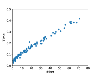
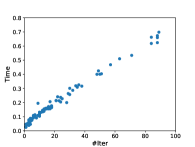
Appendix C Results of Parameter Tuning
We report results of turning parameters on the target model from Env1 using the MNIST images.
| Parameter | Value | Acc | Acc |
|---|---|---|---|
| K-value | 5 | 0.988 | 0.9373 |
| 10 | 0.986 | 0.9465 | |
| 25 | 0.986 | 0.9545 | |
| 50 | 0.985 | 0.962 | |
| 100 | 0.979 | 0.9685 | |
| 150 | 0.977 | 0.9715 | |
| 200 | 0.976 | 0.9753 | |
| Ratio between benign and adversarial examples | 1:0.5 | 0.981 | 0.9643 |
| 1:0.8 | 0.979 | 0.9658 | |
| 1:1 | 0.979 | 0.9685 | |
| 1:1.2 | 0.977 | 0.9705 | |
| 1:2 | 0.971 | 0.9768 | |
| Z-Score | -1 | 0.875 | 0.9918 |
| -1.281552 | 0.926 | 0.987 | |
| -1.644854 | 0.963 | 0.9763 | |
| -1.959964 | 0.979 | 0.9635 | |
| -2 | 0.98 | 0.962 | |
| Statistic Ensemble | 1 | 0.972 | 0.8835 |
| 2 | 0.926 | 0.987 | |
| 3 | 0.883 | 0.994 | |
| 4 | 0.775 | 0.9963 | |
| Classifier | K-NN | 0.979 | 0.9685 |
| SVM | 0.975 | 0.9643 | |
| DTC | 0.994 | 0.9078 | |
| RFC | 0.994 | 0.9068 |
We vary the value of from 5 to 200 for the K-NN based ensemble detector. The results are shown in Table 7, where the bold one denotes the value used in the previous experiments. Column Acc denotes the accuracy on adversarial examples. Column Acc denotes the accuracy on benign examples. We observe that both true and false positive rates slightly increase with the increase of . We also vary the ratio between benign and adversarial examples. As shown in Table 7, with the decrease of the ratio, both true and false positive rates slightly increase.
For the Z-score based ensemble detector, we vary the value of the threshold from -1, -1.281552, -1.644854 and -2, which respectively correspond to about 15%, 10%, 5% and 2.3% false positive rates of 1,000 benign samples. From Table 7, we observe that the smaller the threshold , the lower the false positive rate, but the higher the true positive rate. We also vary the parameter in the Z-score based ensemble detector. Recall that the ensemble detector classifies an input to benign if detectors classify the input to benign, otherwise adversarial. We observe from Table 7 that both true and false positive rates increase with the increase of .
In summary, the above parameters can be used to balance the true and false positive rates, namely, the true positive rate could be improved at the cost of false positive rate.
Finally, instead of K-NN, we also tried the support vector machine (SVM), decision tree (DTC) and random forest (RFC) classification algorithms. We use the implementations of scikit-learn with the default parameters111https://scikit-learn.org. The results in Table 7 show that similar accuracy can be obtained using different classification algorithms. This implies that our detection approach is generic in terms of classification algorithms.
Appendix D More Examples
Figure 11 shows adversarial examples under the attack in Section 6.2.1 with , where each of them except for the benign one targets one of the other labels. All these adversarial examples are successfully detected by A2D + AE.
Figures 12 and 13 show adversarial examples on the adversarially training model with and in Section 6.2.2, where each of them except for the benign ones targets one of the other labels. All the adversarial examples in Figure 12 (i.e., ) can be detected by our defense A2D. Only 3 adversarial examples in Figure 13 (i.e., ) cannot be detected by A2D + AT.
