Towards perturbative renormalization of $\phi^{2}(i\phi)^{\varepsilon}$ quantum field theory

Abstract

In a previous paper it was shown how to calculate the ground-state energy density $\mathcal{E}$ and the $p$-point Green’s functions $G_{p}(x_{1},x_{2},...,x_{p})$ for the $\mathcal{PT}$-symmetric quantum field theory defined by the Hamiltonian density $\mathcal{H}=\mbox{$\textstyle{\frac{1}{2}}$}(\nabla\phi)^{2}+\mbox{$\textstyle{\frac{1}{2}}$}\phi^{2}(i\phi)^{\varepsilon}$ in $D$-dimensional Euclidean spacetime, where $\phi$ is a pseudoscalar field. In this earlier paper $\mathcal{E}$ and $G_{p}(x_{1},x_{2},...,x_{p})$ were expressed as perturbation series in powers of $\varepsilon$ and were calculated to first order in $\varepsilon$. (The parameter $\varepsilon$ is a measure of the nonlinearity of the interaction rather than a coupling constant.) This paper extends these perturbative calculations to the Euclidean Lagrangian $\mathcal{L}=\mbox{$\textstyle{\frac{1}{2}}$}(\nabla\phi)^{2}+\mbox{$\textstyle{\frac{1}{2}}$}\mu^{2}\phi^{2}+\mbox{$\textstyle{\frac{1}{2}}$}g\mu_{0}^{2}\phi^{2}\big{(}i\mu_{0}^{1-D/2}\phi\big{)}^{\varepsilon}-iv\phi$, which now includes renormalization counterterms that are linear and quadratic in the field $\phi$. The parameter $g$ is a dimensionless coupling strength and $\mu_{0}$ is a scaling factor having dimensions of mass. Expressions are given for the one-, two, and three-point Green’s functions, and the renormalized mass, to higher-order in powers of $\varepsilon$ in $D$ dimensions ($0\leq D\leq 2$). Renormalization is performed perturbatively to second order in $\varepsilon$ and the structure of the Green’s functions is analyzed in the limit $D\to 2$. A sum of the most divergent terms is performed to all orders in $\varepsilon$. Like the Cheng-Wu summation of leading logarithms in electrodynamics, it is found here that leading logarithmic divergences combine to become mildly algebraic in form. Future work that must be done to complete the perturbative renormalization procedure is discussed. March 16, 2024

I Introduction

Since the publication of the first paper on $\mathcal{PT}$ symmetry in 1998 r1 , in which the $\mathcal{PT}$-symmetric quantum-mechanical Hamiltonian

$$H=p^{2}+x^{2}(ix)^{\varepsilon}$$ (1)

was introduced, this research area has become highly active. This model has been studied in detail r1-1 , and much theoretical research has been done on the mathematical structure of non-Hermitian quantum systems r1-2 . Beautiful experiments have been performed in diverse areas of physics including optics, photonics, lasers, mechanical and electrical analogs, graphene, topological insulators, superconducting wires, atomic diffusion, NMR, fluid dynamics, metamaterials, optomechanical systems, and wireless power transfer r2 ; r3 ; r4 ; r5 ; r6 ; r7 ; r8 ; r9 ; r10 ; r11 ; r12 ; r13 ; r14 ; r14a .

This paper considers the generalization of (1) to quantum field theory in $D$-dimensional Euclidean space. In an earlier paper r15 we examined the corresponding field-theoretic Lagrangian density

$$\mathcal{L}=\mbox{$\textstyle{\frac{1}{2}}$}(\nabla\phi)^{2}+\mbox{$\textstyle{\frac{1}{2}}$}\phi^{2}(i\phi)^{\varepsilon},$$ (2)

where $\phi$ is a (dimensionless) pseudoscalar field. Note that (2) is manifestly $\mathcal{PT}$-symmetric because $\phi\to-\phi$ under space reflection $\mathcal{P}$ and $i\to-i$ under time reversal $\mathcal{T}$. Just as (1) is a testbed of $\mathcal{PT}$-symmetric quantum mechanics, (2) is a natural model for the study $D$-dimensional $\mathcal{PT}$-symmetric bosonic field theories.

The Hamiltonian (1) launched the field of $\mathcal{PT}$-symmetric quantum theory because it has the surprising feature that if $\varepsilon\geq 0$, its eigenvalues are all discrete, real, and positive even though it is not Dirac-Hermitian r16 ; r17 . (A Dirac-Hermitian Hamiltonian obeys the symmetry constraint $H=H^{\dagger}$, where ${\dagger}$ indicates combined complex conjugation and matrix transposition.) Moreover, the quantum theory defined by (1) is unitary (probability conserving) with respect to the adjoint $\mathcal{CPT}$, where $\mathcal{C}$ is a linear operator satisfying the three simultaneous operator equations r18

$$\mathcal{C}^{2}=1,\quad[\mathcal{C},\mathcal{PT}]=0,\quad[\mathcal{C},H]=0.$$ (3)

Thus, while the constraint that a Hamiltonian be Dirac-Hermitian is sufficient to define a consistent quantum theory, it is not necessary. In short, $\mathcal{PT}$-symmetric quantum theory is not in conflict with the axioms of conventional Hermitian quantum theory; rather, it is a complex generalization of Hermitian quantum theory.

Almost all of the theoretical research on $\mathcal{PT}$ symmetry has focused on $\mathcal{PT}$-symmetric quantum mechanics and experimental studies of $\mathcal{PT}$-symmetric classical systems, but very few papers have focused on $\mathcal{PT}$-symmetric quantum field theory. We briefly review some of the earlier work on $\mathcal{PT}$-symmetric quantum field theory:

1. Early studies of $\mathcal{PT}$-symmetric quantum field theory considered the case $\varepsilon=1$ in (2) r19 ; r20 . This $i\phi^{3}$ quantum field theory had emerged in studies of Reggeon field theory r20a and the Lee-Yang edge singularity r20b . Conventional diagrammatic perturbation theory can be used to treat this cubic interaction: One introduces a coupling constant $g$ in the interaction term $ig\phi^{3}$ and expands the physical quantities in powers of $g$. However, one cannot use conventional perturbation theory for other values of $\varepsilon>0$, integer or noninteger.

2. $\mathcal{PT}$-symmetric electrodynamics also has a cubic interaction r21 . The Johnson-Baker-Willey (JBW) program for constructing a finite massless electrodynamics fails because the zero of the beta function yields at best a negative and perhaps a complex value of $\alpha$ because conventional Hermitian quantum electrodynamics (QED) is not asymptotically free. However, the JBW procedure works for the $\mathcal{PT}$-symmetric version of QED because this theory is asymptotically free and one obtains a reasonable positive numerical value for $\alpha$.

3. Renormalizing a Hermitian quantum field theory often causes the Hamiltonian of the theory to become non-Hermitian. This problem was observed in the Lee model r22 , which is again a theory with a cubic interaction. Pauli and Källén showed that upon renormalization, ghost states (states of negative norm) arise, and appear to violate unitarity in scattering processes. This problem remained unresolved until 2005, when it was shown that if one uses the appropriate $\mathcal{PT}$-symmetric inner product for the renormalized Lee-model Hamiltonian, there are no ghost states and the unitarity of the theory becomes manifest r23 .

4. Renormalizing the Hamiltonian for the Standard Model of particle physics induces what appears to be instability in the vacuum state. This is due to the contribution of the top-quark loop integral r24 . Once again, the renormalized Hamiltonian appears to be non-Hermitian. However, by using $\mathcal{PT}$-symmetric techniques it was shown by using a simple model-field-theory argument that the vacuum state and the next few higher-energy states are actually stable (have real energy) r25 .

5. Introducing higher-order derivatives in a quantum field theory in order to make Feynman integrals converge also makes the Hamiltonian appear to be non-Hermitian. (Higher-order derivatives induce Pauli-Villars ghosts.) However, $\mathcal{PT}$-symmetric techniques resolve this problem. The simplest field-theory model that exhibits this problem is the Pais-Uhlenbeck model and $\mathcal{PT}$-symmetric techniques demonstrate that this theory has no ghosts r26 .

6. The double-scaling limit in quantum field theory [a correlated limit in which the number $N$ of species in an ${\rm O}(N)$-symmetric field theory approaches infinity as the coupling constant approaches a critical value] appears to lead to an unstable field theory. For a quartic scalar field theory the value of $g_{\rm crit}$ is negative and one might think that the resulting $-\phi^{4}$ theory is unstable. However, the techniques of $\mathcal{PT}$-symmetric quantum theory demonstrate that such a theory is actually stable and has a real positive spectrum r27 ; r28 . It was observed by K. Symanzik that a $-\phi^{4}$ theory is asymptotically free even though it does not have a local gauge symmetry but he called this theory “precarious" because it appears to be unstable.

7. Time-like Liouville field theories appear to be unstable and non-Hermitian but the techniques of $\mathcal{PT}$-symmetric quantum field theory can be used to argue that the Hamiltonians of such theories have real spectra and induce unitary time evolution r29 .

8. Studies of the $\mathcal{PT}$-symmetric Dirac equation suggest that one may have species oscillations and still have massless neutrinos r30 ; r31 . Interestingly, recent measurements in Germany have halved the upper bound on the mass of the electron neutrino r31a .

In the studies above some striking results were obtained but many of these field-theory papers considered only simple zero-dimensional toy models and one-dimensional quantum-mechanical analogs that suggest the possible behaviors of $\mathcal{PT}$-symmetric field theories. Thus, there is strong motivation for developing general methods for solving quantum field theories defined by non-Hermitian $\mathcal{PT}$-symmetric Hamiltonians.

Until recently, $\mathcal{PT}$-symmetric quantum field theory has remained beyond the reach of comprehensive analytical study because of three technical problems that had to be overcome when trying to solve the $\mathcal{PT}$-symmetric quantum field theory in (2):

1. Feynman perturbation theory works for the cubic case $\varepsilon=1$ in (2) but for other integer values of $\varepsilon$ the Feynman diagrams must be supplemented by nonperturbative contributions, which are nontrivial. Moreover, when $\varepsilon$ is noninteger, there are no Feynman rules at all so one cannot perform a conventional coupling-constant expansion.

2. The functional integral for the partition function $Z=\int\mathcal{D}\phi\,\exp\big{(}-\int d^{D}x\,\mathcal{L}\big{)}$, does not converge if $\varepsilon>1$ unless the path of integration in function space lies in appropriate infinite-dimensional Stokes sectors in complex field space. Multidimensional Stokes sectors (Lefshetz thimbles r31b ) are unwieldy.

3. In $\mathcal{PT}$-symmetric quantum theory one must use the $\mathcal{C}$ operator, obtained by solving (3), in order to obtain matrix elements. It is difficult to calculate $\mathcal{C}$, so the prospect of calculating Green’s functions appears to be rather dim.

In Ref. r15 it is shown how to overcome these three problems by extending the methods developed in Refs. r32 ; r33 ; r34 for Hermitian quantum field theories to non-Hermitian $\mathcal{PT}$-symmetric quantum field theories. In brief, instead of using a coupling-constant expansion, a perturbation expansion in powers of the parameter $\varepsilon$, which is a measure of the nonlinearity of the theory, is performed and summation methods are then used to evaluate the $\varepsilon$ series. For small $\varepsilon$ the functional integral converges on the real axis in complex-field space, and thus multidimensional Stokes sectors are not required for convergence. This solves problems 1 and 2 above. Expanding in powers of $\varepsilon$ introduces complex logarithms in the functional integrand and $\mathcal{PT}$ symmetry is then enforced by defining the complex logarithm properly:

$$\log(i\phi)\equiv\mbox{$\textstyle{\frac{1}{2}}$}i\pi|\phi|/\phi+\mbox{$\textstyle{\frac{1}{2}}$}\log\big{(}\phi^{2}\big{)}.$$ (4)

The logarithms are now real, and the techniques for handling these logarithms to any order in powers of $\varepsilon$ are based on methods that were introduced in Refs. r32 ; r33 ; r34 .

The apparent problem with the $\mathcal{C}$ operator is actually not a problem if we are calculating Green’s functions. This is because in a theory with an unbroken $\mathcal{PT}$ symmetry the vacuum state is an eigenvalue of $\mathcal{C}$ with eigenvalue 1: $\mathcal{C}|0\rangle=|0\rangle$. Since the Green’s functions are vacuum expectation values, we may ignore problem 3 entirely. This observation was first made in Ref. r36 .

Why does ${\cal L}$ in (2) define an interesting theory? Let us first look at the cubic case. For a conventional $g\phi^{3}$ theory the ground-state energy density $\mathcal{E}$ is a sum of 3-vertex vacuum-bubble Feynman diagrams, and the Feynman perturbation expansion has the form

$$\mathcal{E}=\sum A_{n}g^{2n}.$$

This series diverges and the coefficients $A_{n}$ all have the same sign. Thus, if we perform Borel summation, we find a cut in the Borel plane, which implies that $\mathcal{E}$ is complex. Thus, the vacuum state is unstable. However, to obtain the $\mathcal{PT}$-symmetric cubic theory we replace $g$ by $ig$. Now, the perturbation expansion alternates in sign and the Borel sum of the series is real, the vacuum is stable, and the spectrum of the theory is bounded below.

The case of the quartic $\mathcal{PT}$-symmetric theory is more elaborate. The ground-state energy density for a conventional Hermitian quartic $g\phi^{4}$ quantum field theory has a Feynman perturbation expansion of the form

$$\mathcal{E}=\sum B_{n}(-g)^{n}.$$

Again, this series is divergent, and since the perturbation coefficients $B_{n}$ all have the same sign, the series is alternating and Borel summable. The Borel sum of the perturbation series yields a real value for the vacuum energy density. This implies that the conventional quartic theory has a stable ground state, as one would expect.

It may seem that the $\mathcal{PT}$-symmetric quartic theory obtained by replacing $g$ with $-g$ is problematic because the perturbation series no longer alternates in sign: If we Borel-sum the series, we find a cut in the Borel plane, which suggests that $\mathcal{E}$ is complex and that the vacuum state is unstable, as one might intuitively expect with an upside-down potential. This conclusion is false!

If one examines the functional integral for the partition function of the theory, one sees that the perturbative contribution to $\mathcal{E}$ (the Feynman diagrams) must be supplemented by imaginary nonperturbative contributions arising from two saddle points in complex function space. These additional pure-imaginary contributions exactly cancel the discontinuity in the Borel plane r35 . Consequently, the vacuum state for a $\mathcal{PT}$-symmetric $-g\phi^{4}$ theory is stable. We emphasize that Feynman diagrams alone are not sufficient to calculate the Green’s functions of a $\mathcal{PT}$-symmetric quantum field theory.

The research objectives in this paper are to extend the work in Ref. r15 and to study in depth the problem of renormalization. In Ref. r15 the Lagrangian (2) was examined to first order in $\varepsilon$. Treating $\varepsilon$ as a small perturbation parameter, $\mathcal{L}$ was expanded in a series, which to first order in $\varepsilon$ is

$$\mathcal{L}=\mbox{$\textstyle{\frac{1}{2}}$}(\nabla\phi)^{2}+\mbox{$\textstyle{\frac{1}{2}}$}\phi^{2}+\mbox{$\textstyle{\frac{1}{2}}$}\varepsilon\phi^{2}\log(i\phi)+{\rm O}\big{(}\varepsilon^{2}\big{)}.$$ (5)

Identifying the free Lagrangian as

$$\mathcal{L}_{0}=\mbox{$\textstyle{\frac{1}{2}}$}(\nabla\phi)^{2}+\mbox{$\textstyle{\frac{1}{2}}$}\phi^{2},$$ (6)

we developed techniques to evaluate the shift in the ground-state energy density $\Delta E$ and the Green’s functions $G_{p}$ to first order in $\varepsilon$. We found that

$$\Delta E = \mbox{$\textstyle{\frac{1}{4}}$}\varepsilon(4\pi)^{-D/2}\Gamma\big{(}1-\mbox{$\textstyle{\frac{1}{2}}$}D\big{)}$$ (7)

$$\times\,\big{\{}\log\big{[}2(4\pi)^{-D/2}\Gamma\big{(}1-\mbox{$\textstyle{\frac{1}{2}}$}D\big{)}\big{]}+\psi\big{(}\mbox{$\textstyle{\frac{3}{2}}$}\big{)}\big{\}},$$

$$G_{1} = -i\varepsilon\sqrt{\mbox{$\textstyle{\frac{1}{2}}$}\pi(4\pi)^{-D/2}\Gamma\big{(}1-\mbox{$\textstyle{\frac{1}{2}}$}D\big{)}}.$$ (8)

We then found that the two-point connected Green’s function in momentum space to first order in $\varepsilon$ is

$$\widehat{G}_{2}(p)=1/\big{[}p^{2}+1+\varepsilon K+{\rm O}\big{(}\varepsilon^{2}\big{)}\big{]},$$

where $K=\mbox{$\textstyle{\frac{3}{2}}$}-\mbox{$\textstyle{\frac{1}{2}}$}\gamma+\mbox{$\textstyle{\frac{1}{2}}$}\log\big{[}\mbox{$\textstyle{\frac{1}{2}}$}(4\pi)^{-D/2}\Gamma\big{(}1-\mbox{$\textstyle{\frac{1}{2}}$}D\big{)}\big{]}$. Thus, the renormalized mass to order $\varepsilon$ is

$$M_{R}^{2}=1+K\varepsilon+{\rm O}\big{(}\varepsilon^{2}\big{)}.$$ (9)

In addition, the higher-order connected Green’s functions were also calculated to first order in $\varepsilon$:

$$G_{p}(y_{1},...,y_{p})=-\mbox{$\textstyle{\frac{1}{2}}$}\varepsilon(-i)^{p}\Gamma(\tfrac{p}{2}-1)\big{[}\mbox{$\textstyle{\frac{1}{2}}$}(4\pi)^{-D/2}$$

$$\!\!\!\!\!\!\!\!\!\times\,\Gamma\big{(}1-\mbox{$\textstyle{\frac{1}{2}}$}D\big{)}\big{]}^{1-p/2}\int d^{D}x\prod_{k=1}^{p}\Delta_{1}(y_{k}-x),$$ (10)

where the free propagator $\Delta_{\lambda}(x)$ associated with $\mathcal{L}_{0}=\mbox{$\textstyle{\frac{1}{2}}$}(\nabla\phi)^{2}+\mbox{$\textstyle{\frac{1}{2}}$}\lambda^{2}\phi^{2}$ obeys the general $D$-dimensional Euclidean Klein-Gordon equation

$$\big{(}-\nabla^{2}+\lambda^{2}\big{)}\,\Delta_{\lambda}(x)=\delta^{(D)}(x).$$ (11)

The solution to (11),

$$\Delta_{\lambda}(x)=\lambda^{D/2-1}|x|^{1-D/2}(2\pi)^{-D/2}K_{1-D/2}(\lambda|x|),$$

has the property that

$$\textstyle{\int}d^{D}x\,\Delta_{\lambda}(x)=\lambda^{-2}.$$ (12)

The corresponding selfloop is then

$$\Delta_{\lambda}(0)=\lambda^{D-2}(4\pi)^{-D/2}\Gamma\big{(}1-\mbox{$\textstyle{\frac{1}{2}}$}D\big{)}.$$ (13)

Selfloop factors with $\lambda=1$, which is associated with $\mathcal{L}_{0}$ in (6), enter into (7), (8), and (10) and lead to the factors of $\Gamma\big{(}1-\mbox{$\textstyle{\frac{1}{2}}$}D\big{)}$ that occur in these expressions. This calculation is verified in $D=0$ and $D=1$ in Ref. r15 , where exact calculations are possible, and provides confidence in these perturbative results.

To proceed with the renormalization program we must overcome two problems. First, we must calculate the Green’s functions to higher order in $\varepsilon$. Second, we must show how to renormalize these Green’s functions perturbatively for $D\geq 2$. This paper is focused on renormalization in two dimensions. Specifically, we begin with the formulas for the one-point Green’s function $G_{1}$ in (8) and for the square of the renormalized mass $M_{R}^{2}$ in (9). These quantities are finite for $0\leq D<2$. However, as $D$ approaches $2$ from below ($D\to 2^{-}$) they diverge because $\Gamma(z)$ has a pole at $z=0$: $\Gamma(z)\sim\frac{1}{z}$ as $z\to 0$. Hence, $\Delta_{1}(0)$ in (13) becomes infinite. To study the behavior of $G_{1}$ and $M_{R}^{2}$ near $D=2$ we define $\delta\equiv 2-D$; near $D=2$,

$$\Delta_{1}(0)\sim\tfrac{1}{2\pi\delta}\quad(\delta\to 0)$$ (14)

and the formulas for $G_{1}(\varepsilon)$ and $M_{R}^{2}$ simplify to

$$G_{1}(\varepsilon) \sim -i\varepsilon\tfrac{1}{2\sqrt{\delta}}\quad(\delta\to 0),$$ (15)

$$M_{R}^{2} \sim -\mbox{$\textstyle{\frac{1}{2}}$}\varepsilon\log\delta+A\quad(\delta\to 0),$$ (16)

where $A=1+\varepsilon\big{[}\mbox{$\textstyle{\frac{3}{2}}$}-\frac{\gamma}{2}-\mbox{$\textstyle{\frac{1}{2}}$}\log(4\pi)\big{]}$. From (10) we see that the Green’s functions $G_{p}$ ($p>2$) vanish as $\delta\to 0$, so the theory becomes noninteracting to order $\varepsilon$ at $D=2$.

The question is whether perturbative renormalization can be accomplished in the context of an expansion in powers of the parameter $\varepsilon$. Ordinarily, for interacting bosonic field-theories, renormalization is performed in the context of a coupling-constant expansion. Here, we perform expansions in powers of $\varepsilon$, which is a measure of the nonlinearity of the selfinteraction. Series expansions of this type were introduced many years ago r32 (prior to the study of $\mathcal{PT}$ symmetry), but the problem of renormalization has not been addressed until now.

In our renormalization program, we use the information gained from (15) and (16). The one-point Green’s function $G_{1}$, which is not directly measurable, becomes infinite as $\delta\to 0$. We can remove this divergence by introducing in the Lagrangian a linear counterterm $iv\phi$, where $v$ has dimensions of $({\rm mass})^{1+D/2}$ and $v=v_{1}\varepsilon+v_{2}\varepsilon^{2}+v_{3}\varepsilon^{3}+\cdots$. Such a term is consistent with $\mathcal{PT}$ symmetry if $v$ is real: Under $\mathcal{PT}$ reflection both the pseudoscalar field $\phi$ and $i$ change sign. In addition, the divergence in (16) suggests that we should introduce an (infinite) mass counterterm $\mu$ (the unrenormalized mass) into the Lagrangian. Perturbative mass renormalization then consists of expressing the renormalized mass $M_{R}$ in terms of these Lagrangian parameters and absorbing into the parameter $\mu$ the divergence that arises as $\delta\to 0$.

Thus, we consider the Lagrangian density

$$\mathcal{L}=\mbox{$\textstyle{\frac{1}{2}}$}(\nabla\phi)^{2}+\mbox{$\textstyle{\frac{1}{2}}$}\mu^{2}\phi^{2}+\mbox{$\textstyle{\frac{1}{2}}$}g\mu_{0}^{2}\phi^{2}\big{(}i\mu_{0}^{1-D/2}\phi\big{)}^{\varepsilon}-iv\phi,$$ (17)

that now contains a dimensional field $\phi$, the dimensional parameters $\mu$, $v$, and $\mu_{0}$ (a fixed parameter having dimensions of mass), and the dimensionless unrenormalized coupling $g$. Our objective is to calculate Green’s functions for this quantum field theory as series in powers of the parameter $\varepsilon$ and then to carry out perturbative renormalization for the two-dimensional case. This is a nontrivial extension of the earlier work in which the Green’s functions were calculated to leading order in powers of $\varepsilon$ r15 for the dimensionless Lagrangian density (2).

We thus generalize (2)–(16) to first order in $\varepsilon$. The formula for $G_{1}$ in (8) is modified to read

$$G_{1}(\varepsilon)=-\tfrac{i\varepsilon g}{m^{2}}\mu_{0}^{D/2-1}\sqrt{\mbox{$\textstyle{\frac{1}{2}}$}\pi m^{D-2}\Delta_{1}(0)}+\tfrac{i\varepsilon v_{1}}{\mu_{0}^{2}m^{2}}$$ (18)

and the renormalized mass (9) becomes

$$M_{R}^{2}=(m\mu_{0})^{2}+\mbox{$\textstyle{\frac{1}{2}}$}\varepsilon g\mu_{0}^{2}\big{\{}3-\gamma+\log\big{[}\mbox{$\textstyle{\frac{1}{2}}$}m^{D-2}\Delta_{1}(0)\big{]}\big{\}},$$ (19)

where in both expressions we introduce the dimensionless quantity $m^{2}=g+\mu^{2}/\mu_{0}^{2}$ and we display the new parameters explicitly in terms of $\Delta_{1}(0)$, whose behavior as $\delta\to 0$ is given by (14).

The formulas for $G_{1}(\varepsilon)$ and $M_{R}^{2}$ simplify to

$$G_{1}(\varepsilon) \sim \tfrac{i\varepsilon}{g\mu_{0}^{2}+\mu^{2}}\Big{(}v_{1}-\tfrac{g\mu_{0}^{2}}{2\sqrt{\delta}}\Big{)}\quad(\delta\to 0),$$ (20)

$$M_{R}^{2} \sim \mu^{2}-\mbox{$\textstyle{\frac{1}{2}}$}\varepsilon g\mu_{0}^{2}\log\delta+A\quad(\delta\to 0),$$ (21)

where $A=g\mu_{0}^{2}\big{\{}1+\varepsilon\big{[}\mbox{$\textstyle{\frac{3}{2}}$}-\textstyle{\frac{\gamma}{2}}-\mbox{$\textstyle{\frac{1}{2}}$}\log(4\pi)\big{]}\big{\}}$ is a finite quantity having dimensions of $({\rm mass})^{2}$. By setting $v_{1}=g\mu_{0}^{2}/\big{(}2\sqrt{\delta})$, we remove the divergence in $G_{1}$ as $\delta\to 0$. Next, we see from (21) that the renormalized mass $M_{R}$ is logarithmically divergent as $D\to 2^{-}$. We absorb this divergence into the mass counterterm $\mu$ by setting

$$\mu^{2}=B+\mbox{$\textstyle{\frac{1}{2}}$}\varepsilon g\mu_{0}^{2}\log\delta,$$ (22)

where $B$ is a constant having dimensions of $({\rm mass})^{2}$. (Note that the $\mu^{2}$ counterterm is large and negative.) The renormalized mass is now finite, $M_{R}^{2}=A+B$, and the constant $B$ is in principle determined from the experimental value of the renormalized mass $M_{R}$.

In this paper we study the expansions of the Green’s functions to higher-order in $\varepsilon$ and examine perturbative renormalization in the limit $\delta\to 0$. In Sec. II we use techniques developed in r15 to calculate the connected Green’s functions to order $\varepsilon^{2}$. We examine the effects of the infinite linear and quadratic counterterms $iv\phi$ and $\mu^{2}\phi^{2}$ on the Green’s functions to second order in $\varepsilon$. In Sec. III we perform a multiple-scale analysis in which we obtain the leading contribution to each order in $\varepsilon$ and sum these terms to all orders in $\varepsilon$. We compare the results as $\delta\to 0$ with those obtained via perturbative renormalization. Conclusions are given in Sec. IV.

II Green’s functions to order $\varepsilon^{2}$

The $p$-point Green’s function $G_{p}$ is defined as

$$G_{p}(\varepsilon;y_{1},...,y_{p})=\frac{1}{Z}\int\mathcal{D}\phi\,e^{-\int d^{D}x\,\mathcal{L}}\phi(y_{1})...\phi(y_{p}),$$ (23)

where the Lagrangian (17) enters both in the exponential function in the numerator and in the partition function in the denominator. Expanding the interaction term in powers of $\varepsilon$, we get

$$G_{p}(\varepsilon;y_{1},...,y_{p})=\frac{1}{Z_{0}}\int\!\mathcal{D}\phi\,e^{-\int d^{D}x\,\mathcal{L}_{0}}\phi(y_{1})...\phi(y_{p})$$

$$\!\!\!\!\!\!\!\!\!\!\!\times\exp\bigg{[}\!-\frac{g\mu_{0}^{2}}{2}\sum_{n=1}^{\infty}\frac{\varepsilon^{n}}{n!}\!\int\!\!d^{D}x\,\phi^{2}(x)\log^{n}\big{(}i\mu_{0}^{1-D/2}\phi\big{)}\bigg{]},$$ (24)

where

$$\mathcal{L}_{0}=\mbox{$\textstyle{\frac{1}{2}}$}(\nabla\phi)^{2}+\mbox{$\textstyle{\frac{1}{2}}$}\mu_{0}^{2}m^{2}\phi^{2}.$$ (25)

The Green’s function $G_{p}$ is not connected and to solve the renormalization problem we require the connected $p$-point Green’s functions, which are constructed from cumulants. The procedure to order $\varepsilon$ is explained in detail in Ref. r15 but to second order the cumulants become quite complicated. Of course, the appropriate connected graphs are easy to identify if the expression for $G_{p}$ contains polynomials and not logarithms of the field $\phi$, and in this case standard techniques can then be used to evaluate the graphs. Our strategy here is to recast (24) into a form containing only products of the field $\phi$ at different space-time points. [The expression (24) does not include higher-order terms in $\varepsilon$ that arise from expanding the denominator $Z$ in powers of $\varepsilon$, as these lead to disconnected diagrams.] From here on, in our Green’s function calculations we always discard disconnected contributions to the Green’s functions, and we use the notation $G_{p}$ to represent the connected Green’s functions.

Let us consider terms in $G_{p}(\varepsilon;y_{1},...y_{p})$ to order $\varepsilon^{2}$:

$$G_{p}(\varepsilon;y_{1},...,y_{p}) = \frac{1}{Z_{0}}\int\mathcal{D}\phi\,e^{-\int d^{D}x\,\mathcal{L}_{0}}\phi(y_{1})...\phi(y_{p})$$ (26)

$$\times\big{[}1+\varepsilon g\mu_{0}^{2}I_{1}+\tfrac{1}{2}\varepsilon^{2}g\mu_{0}^{2}\big{(}I_{2}+g\mu_{0}^{2}I_{1}^{2}\big{)}+{\rm O}\big{(}\varepsilon^{3}\big{)}\big{]},$$

where

$$I_{n}=-\mbox{$\textstyle{\frac{1}{2}}$}{\textstyle\int}d^{D}x\,\phi^{2}(x)\log^{n}\big{[}i\mu_{0}^{1-D/2}\phi(x)\big{]}.$$ (27)

Thus, in the expansion of the connected Green’s functions in powers of $\varepsilon$,

$$G_{p}(\varepsilon;y_{1},...,y_{p})=\sum_{n=0}^{\infty}\varepsilon^{n}G_{p,n}(y_{1},...,y_{p}),$$

we identify

$$G_{p,0}\! = \!\frac{1}{Z_{0}}\int\!\!\mathcal{D}\phi\,e^{-\!\int d^{D}x\,\mathcal{L}_{0}}\phi(y_{1})...\phi(y_{p}),$$

$$G_{p,1}\! = \!\frac{g\mu_{0}^{2}}{Z_{0}}\int\!\!\mathcal{D}\phi\,e^{-\!\int d^{D}x\,\mathcal{L}_{0}}\phi(y_{1})...\phi(y_{p})I_{1},$$ (28)

$$G_{p,2}\! = \!\frac{g\mu_{0}^{2}}{2Z_{0}}\int\!\!\mathcal{D}\phi\,e^{-\!\int d^{D}x\,\mathcal{L}_{0}}\phi(y_{1})...\phi(y_{p})\big{(}I_{2}+g\mu_{0}^{2}I_{1}^{2}\big{)},$$

and so on, where we have suppressed the arguments $y_{1},...,y_{p}$ on the left sides.

II.1 One-point Green’s function to second order

The one-point Green’s function can be calculated by adopting the techniques developed in Ref. r15 . Terms odd under $\phi\to-\phi$ integrate to zero, so $G_{1,0}=0$, and $G_{1,1}$, the term proportional to $\varepsilon$, is a constant independent of $y_{1}$. The solution, generalized from Ref. r15 , is

$$G_{1,1}=-igm^{-2}\mu_{0}^{D/2-1}\sqrt{\pi m^{D-2}\Delta_{1}(0)/2},$$ (29)

which is given in (18). In Ref. r15 it is explained how to treat the term $I_{1}$ in (28). This term contains a complex logarithm in $I_{1}=-\mbox{$\textstyle{\frac{1}{2}}$}\int d^{D}x\,\phi^{2}(x)\log\big{[}i\mu_{0}^{1-D/2}\phi(x)\big{]}$ given in (27). The complex logarithm is converted to a real logarithm via (4) and the real logarithm is then treated by applying the replica trick R7

$$\log\big{(}\mu_{0}^{2-D}\phi^{2}\big{)}=\lim_{N\to 0}\,\tfrac{d}{dN}\big{(}\mu_{0}^{1-D/2}\phi\big{)}^{2N},$$ (30)

where the mass constant $\mu_{0}$ keeps the equation dimensionally consistent.

A second insight in r15 concerns terms containing the structure $i|\phi|/\phi$ in (4). Here, we use the integral identity $|\phi|/\phi=(2/\pi)\int_{0}^{\infty}(dt/t)\sin(t\phi)$ and then expand $\sin(t\phi)$ as a Taylor series in powers of $\phi$:

$$\frac{|\phi|}{\phi}=\frac{2}{\pi}\int_{0}^{\infty}dt\!\sum_{\omega=0}^{\infty}\frac{(-1)^{\omega}t^{2\omega}}{(2\omega+1)!}\,\phi^{2\omega+1}.$$ (31)

[Note that the integration variable $t$ has dimensions of $(\rm mass)^{1-D/2}$ so this equation is dimensionally consistent.] Thus, the leading term in the $\varepsilon$ expansion of $G_{1}(\varepsilon)$ is proportional to $\varepsilon$ and was determined to be (18).

The coefficient of $\varepsilon^{2}$ in the expansion of $G_{1}(\varepsilon)$ in (28) is a sum of two functional integrals $G_{1,2}=A_{1}+A_{2}$:

$$A_{1} = -\frac{g\mu_{0}^{2}}{4Z_{0}}\int\mathcal{D}\phi\,e^{-\int d^{D}x\,\mathcal{L}_{0}}\phi(y_{1})$$

$$\leavevmode\nobreak\ \leavevmode\nobreak\ \leavevmode\nobreak\ \times\int d^{D}x\,\phi^{2}(x)\log^{2}\big{[}i\mu_{0}^{1-D/2}\phi(x)\big{]},$$

$$A_{2} = \frac{g^{2}\mu_{0}^{4}}{8Z_{0}}\int\mathcal{D}\phi\,e^{-\int d^{D}x\,\mathcal{L}_{0}}\phi(y_{1})$$ (32)

$$\leavevmode\nobreak\ \leavevmode\nobreak\ \leavevmode\nobreak\ \times\Big{\{}\int d^{D}x\,\phi^{2}(x)\log\big{[}i\mu_{0}^{1-D/2}\phi(x)\big{]}\Big{\}}^{2}.$$

To evaluate $A_{1}$ we insert (4) into (32) to obtain real logarithms and then insert the factor of $\phi^{2}(x)$. Discarding terms odd in $\phi$, we get

$$A_{1} = -\frac{i\pi}{8Z_{0}}g\mu_{0}^{2}\int d^{D}x\int\mathcal{D}\phi\,e^{-\int d^{D}x\,\mathcal{L}_{0}}$$

$$\leavevmode\nobreak\ \leavevmode\nobreak\ \times\,\,\phi(y_{1})|\phi(x)|\phi(x)\log\big{[}\mu_{0}^{2-D}\phi^{2}(x)\big{]}.$$

Next, we use (30) and (31) to replace $|\phi(x)|$ and the logarithm by a sum over products of fields:

$$A_{1}=-\frac{i}{4Z_{0}}g\mu_{0}^{2}\int\!d^{D}x\int\mathcal{D}\phi\,e^{-\int d^{D}x\,\mathcal{L}_{0}}\phi(y_{1})\!\int_{0}^{\infty}\!\!\!dt$$

$$\!\!\!\!\times\,\sum_{\omega=0}^{\infty}\frac{(-1)^{\omega}t^{2\omega}}{(2\omega+1)!}\,\phi^{2\omega+3}(x)\lim_{N\to 0}\frac{d}{dN}\big{[}\mu_{0}^{1-D/2}\phi(x)\big{]}^{2N}.$$

We use graphical techniques to do the functional integral: $A_{1}$ contains products of the fields $\phi(y_{1})\phi^{2\omega+2N+3}(x)$ and represents a free propagator connecting $y_{1}$ to $x$ in $(2\omega+2N+3)$ ways, multiplied by products of selfloops from $x$ to $x$; there are $\omega+N+1$ selfloops. The functional integral yields the value $\Delta(y_{1}-x)\Delta^{\omega+N+1}(0)(2\omega+2N+3)!!$ [For brevity we suppress the mass subscript $\lambda=\mu_{0}m$ in the free propagator $\Delta$ defined in (11).]

We can now perform the $D$-dimensional integral over $x$ and use (12): $\int d^{D}x\,\Delta(y_{1}-x)=\mu_{0}^{-2}m^{-2}$. (Note that the translation invariance of $G_{1}(\varepsilon)$ holds to second order in $\varepsilon$.) Combining these results, we get

$$A_{1}=-\frac{i}{4}{gm^{-2}}\sum_{\omega=0}^{\infty}\int_{0}^{\infty}\!\!\!dt\,\frac{(-t^{2})^{\omega}}{(2\omega+1)!}\Delta^{\omega+1}(0)\lim_{N\to 0}\frac{d}{dN}\big{[}\mu_{0}^{2-D}\Delta(0)\big{]}^{N}(2\omega+2N+3)!!.$$

Taking the derivative with respect to $N$ and the limit $N\to 0$, this simplifies to

$$A_{1}=-\frac{i}{4}{gm^{-2}}\sum_{\omega=0}^{\infty}\int_{0}^{\infty}\!\!\!dt\,\frac{(-t^{2})^{\omega}}{(2\omega+1)!}\Delta^{\omega+1}(0)(2\omega+3)!!\big{\{}\log\big{[}2\mu_{0}^{2-D}\Delta(0)\big{]}+\psi\big{(}\omega+\tfrac{5}{2}\big{)}\big{\}},$$ (33)

where we use the duplication formula for the digamma function $\psi(2z)=\mbox{$\textstyle{\frac{1}{2}}$}\psi(z)+\mbox{$\textstyle{\frac{1}{2}}$}\psi\big{(}z+\mbox{$\textstyle{\frac{1}{2}}$}\big{)}+\log 2$. To evaluate the sum and integral we use r15

$$\int_{0}^{\infty}\!\!\!dt\,\sum_{\omega=0}^{\infty}\frac{(-t^{2})^{\omega}}{(2\omega+1)!}\Delta^{\omega+1}(0)(2\omega+3)!!=\Delta(0)\int_{0}^{\infty}\!\!\!dt\,\big{[}3-\Delta(0)t^{2}\big{]}e^{-\Delta(0)t^{2}/2}=\sqrt{2\pi\Delta(0)}.$$ (34)

To calculate the second term in (33) we insert the integral representation R8

$$\textstyle{\psi(a)=\int_{0}^{\infty}dz\Big{(}\frac{e^{-z}}{z}-\frac{e^{-az}}{1-e^{-z}}\Big{)}},$$

perform the sum over $\omega$ and the integral over $t$, and then note that the $z$ integral gives the factor $\psi(2)$. Thus,

$$\int_{0}^{\infty}\!\!\!\!dt\sum_{\omega=0}^{\infty}\!\!\frac{(-t^{2})^{\omega}}{(2\omega+1)!}\Delta^{\omega+1}(0)(2\omega+3)!!\psi\big{(}\omega+\tfrac{5}{2}\big{)}$$

$$\leavevmode\nobreak\ \leavevmode\nobreak\ \leavevmode\nobreak\ \leavevmode\nobreak\ =\sqrt{2\pi\Delta(0)}\,\psi(2).$$ (35)

Combining (34) and (35), we obtain $A_{1}$ from (33):

$$A_{1}=-\tfrac{i}{2}gm^{-2}\sqrt{\tfrac{\pi\Delta(0)}{2}}\Big{\{}\log\big{[}2\mu_{0}^{2-D}\Delta(0)\big{]}+\psi(2)\Big{\}}.$$ (36)

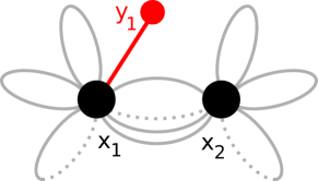
((a))

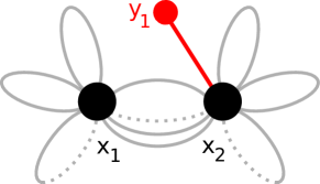
((b))

Figure 1: Graphical representation of terms contributing to the functional integrals in (37). In 1(a), the line joining the external point $y_{1}$ to the internal point $x_{1}$ is one of an odd number of lines meeting at $x_{1}$; an even number of lines are connected to the internal point $x_{2}$. In 1(b) the line from the external point $y_{1}$ is one of an even number of points at $x_{2}$; and odd number of lines connect to $x_{1}$. We integrate over the internal points $x_{1}$ and $x_{2}$.

Next, we evaluate $A_{2}$ in (32). Expanding $I_{1}^{2}$ produces fields $\phi$ at two points, say $x_{1}$ and $x_{2}$, which are integrated over. As before, we replace each occurrence of an imaginary logarithm by using (4) and retain terms that are even in $\phi$. (The functional integral vanishes for terms that are odd in $\phi$.) Only one term survives:

$$A_{2} = \tfrac{i\pi g^{2}\mu_{0}^{4}}{16Z_{0}}\int\mathcal{D}\,\phi e^{-\int d^{D}x\mathcal{L}_{0}}\phi(y_{1})\int\!d^{D}x_{1}\!\int\!d^{D}x_{2}$$

$$\leavevmode\nobreak\ \leavevmode\nobreak\ \times\,\phi(x_{1})|\phi(x_{1})|\phi^{2}(x_{2})\log\big{[}\mu_{0}^{2-D}\phi^{2}(x_{2})\big{]}.$$

Using (31) to replace $\phi(x_{1})|\phi(x_{1})|$ and the replica trick (30) to replace the logarithm, we express $A_{2}$ as:

$$A_{2} = \frac{ig^{2}\mu_{0}^{4}}{8Z_{0}}\int\!d^{D}x_{1}\!\int\!d^{D}x_{2}\int_{0}^{\infty}\!\!\!dt\!\sum_{\omega=0}^{\infty}\frac{(-t^{2})^{\omega}}{(2\omega+1)!}$$ (37)

$$\!\!\!\!\!\!\!\!\!\!\!\!\times\,\int\!\mathcal{D}\phi\,e^{-\int d^{D}x\,\mathcal{L}_{0}}\phi(y_{1})\phi^{2\omega+3}(x_{1})\phi^{2}(x_{2})$$

$$\!\!\!\!\!\!\!\!\!\!\!\!\times\lim_{N\to 0}\frac{d}{dN}\big{[}\mu_{0}^{1-D/2}\phi(x_{2})\big{]}^{2N}.$$

Here we must evaluate the functional integral that connects the field at the external point $y_{1}$ to one of the (odd number of) fields at the internal points $x_{1}$; the remaining (even number of) points must be connected to the even number of points at $x_{2}$. To this we must add the result of connecting the external point $y_{1}$ to the (even number of) points at $x_{2}$ leaving an odd number of connections from $x_{2}$ to $x_{1}$. This includes all connected diagrams illustrated schematically in Figs. 1(a) and 1(b).

The path integral corresponding to Fig. 1(a), for the field combinations $\phi(y_{1})\phi^{2\omega+3}(x_{1})\phi^{2N+2}(x_{2})$ allows $y_{1}$ to connect to one of the $2\omega+3$ replicas of $\phi$ at $x_{1}$. For the remaining points to be connected, $2l$ lines can connect the remaining $2\omega+2$ points at $x_{1}$ to the $2N+2$ points at $x_{2}$; the remainder of points $(2N+2-2l)+(2\omega+2-2l)$ are used to form $N+\omega+2-2l$ closed loops. Here, $l\geq 1$ for the graph to be connected. We assign to Fig. 1(a) the combinatoric factor

$$C_{a}=\textstyle{\frac{(2N+2)!(2\omega+3)!}{(2l)!(N+1-l)!(\omega+1-l)!2^{N+\omega+2-2l}}}.$$

For Fig. 1(b) there are $2N+2$ ways to connect $y_{1}$ to $x_{2}$. To create connected graphs an odd number, say $2l+1$, of lines must join the remaining $2N+1$ points at $x_{1}$ to the $2\omega+3$ points at $x_{2}$, where the minimum value of $l$ is zero. Closed loops can exist on $2N+1-(2l+1)=2N-2l$ points on $x_{2}$ and $2\omega+3-(2l+1)$ points on $x_{1}$, forming a total of $N+\omega-2l+1$ loops. The combinatoric factor assigned to this graph is

$$C_{b}=\textstyle{\frac{(2N+2)!(2\omega+3)!}{(2l+1)!(N-l)!(\omega+1-l)!2^{N+\omega+1-2l}}}.$$

It is best to examine the contributions from Fig. 1(a) and Fig. 1(b) separately. We use the combinatoric factor $C_{a}$ associated with Fig. 1(a) to evaluate its contribution to (37) and perform one spatial integral:

$$A_{2}^{\rm Fig.\,1a} = \frac{ig^{2}\mu_{0}^{2}}{8m^{2}}\lim_{N\to 0}\frac{d}{dN}(2N+2)!\big{[}\mbox{$\textstyle{\frac{1}{2}}$}\mu_{0}^{2-D}\Delta(0)\big{]}^{N}\int d^{D}x\int_{0}^{\infty}dt\sum_{\omega=0}^{\infty}(-t^{2})^{\omega}(2\omega+3)(2\omega+2)\big{[}\mbox{$\textstyle{\frac{1}{2}}$}\Delta(0)\big{]}^{\omega+2}$$ (38)

$$\times\sum_{l=1}^{min(N+1,\,\omega+1)}\frac{1}{(2l)!(N+1-l)!(\omega+1-l)!}\Big{[}2\tfrac{\Delta(x)}{\Delta(0)}\Big{]}^{2l}.$$

Exchanging the sums on $l$ and $\omega$ with $\omega\geq l-1$, we determine the sum over $\omega$:

$$\sum_{\omega=l-1}^{\infty}(-z)^{\omega}\frac{(2\omega+3)(2\omega+2)}{(\omega+1-l)!}=(-z)^{l-1}e^{-z}\big{[}4z^{2}-z(8l+6)+2l(2l+1)\big{]},$$

where we have shifted the summation variable to $p=\omega+1-l$, which runs from $0$ to $\infty$, and we have used the sums $\sum_{p}z^{p}/p!=e^{z}$, $\sum_{p}pz^{p}/p!=ze^{z}$, and $\sum_{p}p^{2}z^{p}/p!=(z^{2}+z)e^{z}$.

Setting $z=\mbox{$\textstyle{\frac{1}{2}}$}\Delta(0)t^{2}$ we evaluate the integral over $t$:

$$\int_{0}^{\infty}\!\!dt\sum_{\omega=l-1}^{\infty}\big{[}-\mbox{$\textstyle{\frac{1}{2}}$}\Delta(0)t^{2}\big{]}^{\omega}\frac{(2\omega+3)(2\omega+2)}{(\omega+1-l)!}=2\frac{(-1)^{l-1}}{\sqrt{2\Delta(0)}}\Gamma\big{(}l-\mbox{$\textstyle{\frac{1}{2}}$}\big{)}.$$ (39)

Thus, (38) becomes

$$A_{2}^{\rm Fig.\,1a}=\frac{ig^{2}\mu_{0}^{2}}{4\sqrt{2}m^{2}}[\Delta(0)]^{3/2}\lim_{N\to 0}\frac{d}{dN}(2N+2)!\big{[}\mbox{$\textstyle{\frac{1}{2}}$}\mu_{0}^{2-D}\Delta(0)\big{]}^{N}\int d^{D}x\sum_{l=1}^{\infty}\big{[}\tfrac{\Delta(x)}{\Delta(0)}\big{]}^{2l}\frac{(-1)^{l-1}\Gamma\big{(}l-\mbox{$\textstyle{\frac{1}{2}}$}\big{)}}{2^{2-2l}(2l)!(N+1-l)!}.$$ (40)

To evaluate the sum over $l$ we simplify the factorials and Gamma functions by using the duplication formula $\Gamma(2z)=\Gamma(z)\Gamma\big{(}z+\mbox{$\textstyle{\frac{1}{2}}$}\big{)}2^{2z-1}/\sqrt{\pi}$ and Euler’s reflection formula $\Gamma(z)\Gamma(1-z)=\pi/\sin(\pi z)$. Then (40) reduces to

$$A_{2}^{\rm Fig.\,1a}=\frac{ig^{2}\mu_{0}^{2}}{m^{2}}\big{[}\mbox{$\textstyle{\frac{1}{2}}$}\Delta(0)\big{]}^{3/2}\lim_{N\to 0}\frac{d}{dN}[2\mu_{0}^{2-D}\Delta(0)]^{N}\Gamma\big{(}N+\tfrac{3}{2}\big{)}\int d^{D}x\Big{\{}{}_{2}F_{1}\big{(}-\mbox{$\textstyle{\frac{1}{2}}$},-N-1;\mbox{$\textstyle{\frac{1}{2}}$};\Big{[}\tfrac{\Delta(x)}{\Delta(0)}\Big{]}^{2}\big{)}-1\Big{\}},$$ (41)

where ${}_{2}F_{1}\big{(}a,b;c;x^{2}\big{)}$ is a Gaussian hypergeometric function R8 . When $N=0$ this function becomes simply ${}_{2}F_{1}\big{(}-\mbox{$\textstyle{\frac{1}{2}}$},-1;\mbox{$\textstyle{\frac{1}{2}}$};x^{2}\big{)}=1+x^{2}$ and $\lim_{N\to 0}\frac{d}{dN}\,{}_{2}F_{1}\big{(}-\mbox{$\textstyle{\frac{1}{2}}$},-N-1;\mbox{$\textstyle{\frac{1}{2}}$};x^{2}\big{)}=(1+x)^{2}\log(1+x)+(1-x)^{2}\log(1-x)-2x^{2}$.

Next, evaluate the contribution from Fig. 1(b). Multiplying the combinatorial factor $C_{b}$ with the associated propagators in the evaluation of the functional integral of (37) and performing one spatial integration, we get

$$A_{2}^{\rm Fig.\,1b} = \frac{ig^{2}\mu_{0}^{2}}{8m^{2}}\lim_{N\to 0}\frac{d}{dN}(2N+2)!\big{[}\mbox{$\textstyle{\frac{1}{2}}$}\mu_{0}^{2-D}\Delta(0)\big{]}^{N}\int d^{D}x\int_{0}^{\infty}dt\sum_{\omega=0}^{\infty}(-1)^{\omega}t^{2\omega}(2\omega+3)(2\omega+2)\big{[}\mbox{$\textstyle{\frac{1}{2}}$}\Delta(0)\big{]}^{\omega}$$

$$\times\sum_{l=0}^{min(N,\omega+1)}[\Delta(x)]^{2l+1}\big{[}\mbox{$\textstyle{\frac{1}{2}}$}\Delta(0)\big{]}^{1-2l}\frac{1}{(2l+1)!(N-l)!(\omega+1-l)!}$$

Exchanging orders of summation over $l$ and $\omega$ and using (39) to sum over $\omega$ and integrate over $t$, we obtain

$$A_{2}^{\rm Fig.\,1b}=\frac{ig^{2}\mu_{0}^{2}}{4\sqrt{2}m^{2}}[\Delta(0)]^{3/2}\lim_{N\to 0}\frac{d}{dN}[\mbox{$\textstyle{\frac{1}{2}}$}\mu_{0}^{2-D}\Delta(0)]^{N}(2N+2)!\int d^{D}x\sum_{l=0}^{\infty}\Big{[}\tfrac{\Delta(x)}{\Delta(0)}\Big{]}^{2l+1}\frac{(-1)^{l-1}\Gamma(l-\tfrac{1}{2})}{2^{1-2l}(2l+1)!(N-l)!}.$$

Again, on applying the duplication and reflection formulas for the Gamma function, we find that this expression also simplifies to the compact form

$$A_{2}^{\rm Fig.\,1b}=\frac{2ig^{2}\mu_{0}^{2}}{m^{2}}\big{[}\mbox{$\textstyle{\frac{1}{2}}$}\Delta(0)\big{]}^{3/2}\lim_{N\to 0}\frac{d}{dN}[2\mu_{0}^{2-D}\Delta(0)]^{N}(N+1)\Gamma\big{(}N+\tfrac{3}{2}\big{)}\int d^{D}x\frac{\Delta(x)}{\Delta(0)}\,{}_{2}F_{1}\Big{(}-\mbox{$\textstyle{\frac{1}{2}}$},-N;\tfrac{3}{2};\big{[}\tfrac{\Delta(x)}{\Delta(0)}\big{]}^{2}\Big{)}.$$ (42)

When $N=0$, the hypergeometric function simplifies, ${}_{2}F_{1}\big{(}-\mbox{$\textstyle{\frac{1}{2}}$},0;\mbox{$\textstyle{\frac{3}{2}}$};x^{2}\big{)}=1$, and its derivative at $N=0$ is $\lim_{N\to 0}\,\frac{d}{dN}{}_{2}F_{1}\big{(}-\mbox{$\textstyle{\frac{1}{2}}$},-N;\,\mbox{$\textstyle{\frac{3}{2}}$};x^{2}\big{)}=\frac{1}{2x}[(1+x)^{2}\,\log(1+x)-(1-x)^{2}\,\log(1-x)-2x].$ Thus, $A_{2}=A_{2}\,[{\rm Fig.\,1a}]+A_{2}\,[{\rm Fig.\,1b}]$ is constructed by adding (41) and (42), yielding the formal result

$$A_{2} = \frac{ig^{2}\mu_{0}^{2}}{m^{2}}[\tfrac{1}{2}{\Delta(0)}]^{3/2}\lim_{N\to 0}\frac{d}{dN}[2\mu_{0}^{2-D}\Delta(0)]^{N}\,\Gamma\big{(}N+\mbox{$\textstyle{\frac{3}{2}}$}\big{)}$$

$$\times \int d^{D}x\Big{[}\big{(}{}_{2}F_{1}\Big{(}-\mbox{$\textstyle{\frac{1}{2}}$},-N-1;\mbox{$\textstyle{\frac{1}{2}}$};\big{[}\tfrac{\Delta(x)}{\Delta(0)}\big{]}^{2}\,\Big{)}-1\big{)}+2(N+1)\tfrac{\Delta(x)}{\Delta(0)}\,{}_{2}F_{1}\Big{(}-\mbox{$\textstyle{\frac{1}{2}}$},-N;\mbox{$\textstyle{\frac{3}{2}}$};\Big{[}\tfrac{\Delta(x)}{\Delta(0)}\Big{]}^{2}\Big{)}\Big{]}$$

$$= \tfrac{ig^{2}\mu_{0}^{2}\sqrt{\pi}}{2m^{2}}\big{[}\mbox{$\textstyle{\frac{1}{2}}$}\Delta(0)\big{]}^{3/2}\Big{\{}\big{[}\log[2\mu_{0}^{2-D}\Delta(0)]+\psi\big{(}\mbox{$\textstyle{\frac{3}{2}}$}\big{)}\big{]}\!\!\int d^{D}x\Big{(}\big{[}\tfrac{\Delta(x)}{\Delta(0)}\big{]}^{2}+2\tfrac{\Delta(x)}{\Delta(0)}\Big{)}$$

$$\quad+2\int d^{D}x\,\Big{[}\big{(}1+\tfrac{\Delta(x)}{\Delta(0)}\big{)}^{2}\log\big{[}1+\tfrac{\Delta(x)}{\Delta(0)}i\big{]}-\big{[}\tfrac{\Delta(x)}{\Delta(0)}\big{]}^{2}\Big{]}\Big{\}}.$$

The integrals containing linear and quadratic powers of $\Delta(x)$ are readily evaluated, the linear one following from (12), and the quadratic one from the solution to (10), using $\int_{0}^{\infty}dt\,tK^{2}_{\nu}(t)=\mbox{$\textstyle{\frac{1}{2}}$}\Gamma(1-\nu)\Gamma(1+\nu)$. This yields $\int d^{D}x\,[\Delta(x)]^{2}=(\mu_{0}m)^{D-4}2^{-D}\pi^{-D/2}\Gamma(2-D/2)$. Thus,

$$A_{2}=\tfrac{i}{8}g^{2}m^{-4}\sqrt{\pi\Delta(0)/2}\big{\{}\big{[}\log[2\mu_{0}^{2-D}\Delta(0)]+\psi(\tfrac{3}{2})\big{]}(6-D)+2D-4+4\Delta(0)\mu_{0}^{2}m^{2}\!\int\!d^{D}x\,\big{(}1+\tfrac{\Delta(x)}{\Delta(0)}\big{)}^{2}\log\big{[}1+\tfrac{\Delta(x)}{\Delta(0)}\big{]}\big{\}}.$$

The connected part of $G_{1}$ to order $\varepsilon^{2}$ is $A_{1}+A_{2}$, so we add the above result to (36) to get

$$G_{1,2} = -\mbox{$\textstyle{\frac{1}{2}}$}igm^{-2}\sqrt{\mbox{$\textstyle{\frac{1}{2}}$}\pi\Delta(0)}\Big{\{}\log[2\mu_{0}^{2-D}\Delta(0)]+\psi(2)\Big{\}}+\tfrac{1}{8}ig^{2}m^{-4}\sqrt{\mbox{$\textstyle{\frac{1}{2}}$}\pi\Delta(0)}\Big{\{}\big{(}\log[2\mu_{0}^{2-D}\Delta(0)]+\psi(\tfrac{3}{2})\big{)}(6-D)$$

$$\qquad+2D-4+4\Delta(0)\mu_{0}^{2}m^{2}\int d^{D}x\,\big{(}1+\tfrac{\Delta(x)}{\Delta(0)}\big{)}^{2}\log\big{[}1+\tfrac{\Delta(x)}{\Delta(0)}\big{]}\Big{\}}.$$

The first term is proportional to the dimensionless coupling strength $gm^{-2}$ while the second term is proportional to its square. In the second term the expression in curly brackets is a dimensionless number.

We now examine the limit $D\to 2$ (that is, $\delta\to 0$). From the solution to (11) and (13) we see that the combination $\Delta(x)/\Delta(0)\sim\delta K_{0}(\mu_{0}m|x|)$ to first order in $\delta$ as $\delta\to 0$. Thus, to lowest order in $\delta$ the last term containing the integral simplifies to

$$4\Delta(0)\mu_{0}^{2}m^{2}\int d^{D}x\,\Big{(}1+\frac{\Delta(x)}{\Delta(0)}\Big{)}^{2}\log\Big{[}1+\tfrac{\Delta(x)}{\Delta(0)}\Big{]}$$

$$\sim 4\mu_{0}^{2}m^{2}\int_{0}^{\infty}dx\,xK_{0}(\mu_{0}m|x|)=4$$

because $\int_{0}^{\infty}dt\,t^{\alpha-1}K_{\nu}(t)=2^{\alpha-2}\Gamma(\tfrac{\alpha-\nu}{2})\Gamma(\frac{\alpha+\nu}{2})$, ${\rm Re}\,\alpha>|{\rm Re}\,\nu|$. Thus, if $D\to 2$, the coefficient of $G_{1}$ at second order in $\varepsilon$ goes as

$$G_{1,2} \sim -\tfrac{i}{4}gm^{-2}\delta^{-1/2}[\psi(2)-\log(\pi\delta)]$$

$$\!\!\!\!\!\!+\tfrac{i}{4}g^{2}m^{-4}\delta^{-1/2}\big{[}1+\psi(\tfrac{3}{2})-\log\pi-\log\delta\big{]}+{\rm O}(\delta).$$

Taking the same limit in (29), the coefficient of $G_{1}$ to first order in $\varepsilon$ yields $G_{1,1}\to-\mbox{$\textstyle{\frac{1}{2}}$}igm^{-2}\delta^{-1/2}$. Putting these two last results together, we find that the divergence structure of $G_{1}$ in the $\varepsilon$ expansion has the form

$$G_{1}\to-ic_{1}\delta^{-1/2}\varepsilon-i\delta^{-1/2}(c_{2}+c_{3}\log\delta)\varepsilon^{2}+{\rm O}(\varepsilon^{3}),$$

where $c_{1}=\mbox{$\textstyle{\frac{1}{2}}$}gm^{-2}$, $c_{2}=\mbox{$\textstyle{\frac{1}{4}}$}gm^{-2}\big{[}\psi(2)-\log\pi-gm^{-2}\big{(}1+\psi\big{(}\tfrac{3}{2}\big{)}-\log\pi\big{)}\big{]}$, and $c_{3}=-\mbox{$\textstyle{\frac{1}{4}}$}gm^{-2}(1-gm^{-2})$ are constants. So, the algebraic divergence $\delta^{-1/2}$ occurs at each order in the $\varepsilon$ expansion. Our key result is that the second-order term in the $\varepsilon$ expansion introduces $\log\delta$ but does not alter the algebraic structure of the divergence.

Inclusion of the counterterm $-iv\phi$. As seen from the calculations above, $G_{1}$ is negative imaginary and diverges in two dimensions as $\delta\to 0$. Since $G_{1}$ is not a physically measurable quantity, it can be removed by introducing an appropriate counterterm $-iv\phi$ into the Lagrangian, where $v=v_{1}\varepsilon+v_{2}\varepsilon^{2}+{\rm O}(\varepsilon^{3})$.

To examine the effect of including such a term, we denote the one-point connected Green’s function associated with the full Lagrangian that includes $-iv\phi$ as $G_{1}(v)$. Its relation to the Green’s functions evaluated without $v$ is determined as follows. [We keep the notation of this section, without explicitly writing $v=0$; that is, $G_{1}(v=0)=G_{1}$ and similarly for the higher-order Green functions and all expansion coefficients.] We include the contributions to the path integral of $\exp\big{[}i\int d^{D}x\big{(}v_{1}\varepsilon+v_{2}\varepsilon^{2}\big{)}\phi(x)\big{]}$ to second order in $\varepsilon$. This multiplies the expansion in $\varepsilon$ of $G_{p}$ in (26). Identifying terms proportional to $\varepsilon$ and $\varepsilon^{2}$ and using the definitions in (28), we find that for any $p$

$$G_{p}(v) = G_{p,0}+\varepsilon\Big{[}G_{p,1}+iv_{1}\!\int\!\!d^{D}x\,G_{p+1,0}(y_{1},...y_{p},x)\Big{]}$$ (43)

$$+ \varepsilon^{2}\Big{[}G_{p,2}+iv_{2}\int d^{D}x\,G_{p+1,0}(y_{1},...,y_{p},x)$$

$$- \frac{1}{2}v_{1}^{2}\int d^{D}x_{1}\int d^{D}x_{2}G_{p+2,0}(y_{1},...,y_{p},x_{1},x_{2})$$

$$+ iv_{1}\int d^{D}xG_{p+1,1}(y_{1},...,y_{p},x)\Big{]}+{\rm O}\big{(}\varepsilon^{3}\big{)},$$

where we have suppressed the arguments $y_{1},...,y_{p}$ of $G_{p,n}$. Thus, the coefficients of the $\varepsilon$ expansion $G_{p}(v)=\sum_{n}\varepsilon^{n}G_{p,n}(v)$ are related to the coefficients of the expansion of $G_{p}$ through the above expression. In principle, if we calculate the coefficients in the $\varepsilon$ expansion of the Green’s function without $v$, we can easily determine the effects of including it.

Let us evaluate $G_{1}(v)$. From (43) we get

$$G_{1}(v) = \varepsilon\Big{[}G_{1,1}+iv_{1}\int d^{D}x\,G_{2,0}(y,x)\Big{]}+\varepsilon^{2}\Big{[}G_{1,2}$$

$$\!\!\!\!\!\!\!\!\!\!\!\!\!\!\!+iv_{2}\int d^{D}x\,G_{2,0}(y,x)+iv_{1}\int d^{D}x\,G_{2,1}(y,x)\Big{]},$$

since $G_{p,0}=0$ unless $p=2$. Thus, to evaluate $G_{1}(v)$ to second order in $\varepsilon$, we must know the expansion coefficients of the two-point Green’s function, calculated to first-order in $\varepsilon$ without $v$. But these are known; by definition, $G_{2,0}(y,x)=\Delta(y-x)$ while

$$G_{2,1}(y,x)=-g\mu_{0}^{2}K_{1}\int d^{D}z\,\Delta(y-z)\Delta(z-x),$$ (44)

with $K_{1}=3/2-\gamma/2+\mbox{$\textstyle{\frac{1}{2}}$}\log\big{[}\mu_{0}^{2-D}\Delta(0)/2\big{]}$ is a generalization of the result obtained in r15 that includes the mass parameter $\mu_{0}m$ of the Lagrangian $\mathcal{L}_{0}$ used here [see (25)]. In the limit $\delta\to 0$, $G_{1,1}\to-igm^{-2}/(2\sqrt{\delta})$ from (29), so in this limit

$$G_{1}(v) \sim i\varepsilon\Big{(}\frac{v_{1}}{\mu_{0}^{2}m^{2}}-\frac{g}{2m^{2}\sqrt{\delta}}\Big{)}$$ (45)

$$\!\!\!\!\!\!\!\!\!\!\!\!\!\!\!\!\!\!\!\!\!\!\!\!\!\!\!+i\varepsilon^{2}\Big{[}\frac{v_{2}}{\mu_{0}^{2}m^{2}}-\frac{gK_{1}v_{1}}{\mu_{0}^{2}m^{4}}-\delta^{-1/2}(c_{2}+c_{3}\log\delta)\Big{]}.$$

Setting $G_{1}(v)=0$, we obtain the first-order result in (20), which fixes $v_{1}\to g\mu_{0}^{2}/(2\sqrt{\delta})$. If we insert this into (45), then $v_{2}$ in turn is fixed to eliminate the ${\rm O}\big{(}\varepsilon^{2}\big{)}$ term. It too has the same divergence structure $v_{2}\to\delta^{-1/2}$.

In summary, from our ${\rm O}\big{(}\varepsilon^{2}\big{)}$ calculation of $G_{1}$, we find that the divergence structure obtained when $D\to 2$ has the same algebraic form that was determined from the ${\rm O}(\varepsilon)$ term; namely, $\delta^{-1/2}$. It is accompanied by a logarithmic divergence in $\delta$. This is a structure that persists for higher-order Green’s functions. We will see that as $D\to 2$, the algebraic structure of the lowest-order Green’s functions is accompanied by logarithmic divergences as one goes to higher orders in the $\varepsilon$ expansion.

II.2 Two-point Green’s function in second order

A general expression for the $p$-point Green’s functions and their coefficients in the $\varepsilon$ expansion, given in (26)–(28) can be formulated using the generalized form of the replica trick (30)

$$\log^{m}\big{[}\mu_{0}^{2-D}\phi^{2}\big{]}=\lim_{N\to 0}\,(\tfrac{d}{dN})^{m}\big{(}\mu_{0}^{1-D/2}\phi\big{)}^{2N}$$

and the generalization of (31),

$$\Big{(}\frac{|\phi|}{\phi}\Big{)}^{m}=\frac{2}{\pi}\int_{0}^{\infty}\!\!dt\sum_{\omega=0}^{\infty}\frac{\big{(}-t^{2}\big{)}^{\omega}}{(2\omega+1)!}\,\phi^{(2\omega+1)m}.$$

Before applying these, expressions containing $I_{n}$ will have the occurrence of $\log^{n}\big{[}i\mu_{0}^{1-D/2}\phi(x)\big{]}$ in (27) written in terms of real logarithms via (4) and expanded in a binomial series. As illustrated in detail in the previous section, the aim is to reduce the expressions that arise to products of functional integrals containing powers of $\phi$ multiplied by appropriate factors.

From (28) the lowest-order contribution to $G_{2}(y_{1},y_{2})$ is the free Green’s function $G_{2,0}(y_{1},y_{2})=\Delta(y_{1}-y_{2})$. Performing the operations delineated in the last section, the coefficient of $\varepsilon$ becomes

$$G_{2,1}(y_{1},y_{2}) = -\frac{g\mu_{0}^{2}}{4}\int d^{D}x\lim_{N\to 0}\frac{d}{dN}\mu_{0}^{(2-D)N}$$ (46)

$$\!\!\!\!\!\!\!\!\!\!\!\!\!\!\!\!\!\!\!\!\!\!\!\!\!\!\!\!\times\int\frac{\mathcal{D}\phi}{Z_{0}}\,e^{-\int d^{D}x\,\mathcal{L}_{0}}\phi(y_{1})\phi(y_{2})\phi^{2N+2}(x),$$

where the connected graph associated with the functional integral connects the two external points to one internal one (see Fig. 2). In this case the functional integral takes the value $[(2N+2)!/(2^{N}N!)][\Delta(0)]^{N}\Delta(y_{1}-x)\Delta(x-y_{2})$, leading to the final result given in (44).

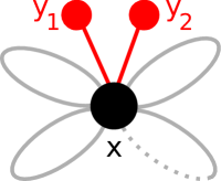
Figure 2: Graphical representation of connected terms contributing to the functional integrals in (46) and (47).

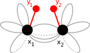
((a))

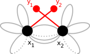
((b))

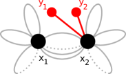
((c))

((d))

Figure 3: Graphical representation of terms contributing to the functional integrals in (48). In 3(a), $y_{1}$ ($y_{2}$) connects to the point $x_{1}$ ($x_{2}$), with the remaining number of points connecting $x_{1}$ to $x_{2}$. In 3(b) the connection of $y_{1}$ ($y_{2}$) is to the points at $x_{2}$ ($x_{1}$), with the remaining points connecting to $x_{1}$ to $x_{2}$. In 3(c) and 3(d) both $y_{1}$ and $y_{2}$ are connected to the same point, either $x_{1}$ or $x_{2}$, with these being connected. $x_{1}$ and $x_{2}$ are integrated over.

In the $\varepsilon$ expansion of $G_{2}(y_{1},y_{2})$, the coefficient proportional to $\varepsilon^{2}$, has the form $G_{2,2}=A_{2;1}+A_{2;2}$, where

$$A_{2;1} = -\frac{g\mu_{0}^{2}}{4Z_{0}}\int\mathcal{D}\phi\,e^{-\int d^{D}x\,\mathcal{L}_{0}}\phi(y_{1})\phi(y_{2})$$ (47)

$$\times\int d^{D}x\,\phi^{2}(x)\log^{2}\big{[}i\mu_{0}^{1-D/2}\phi(x)\big{]},$$

$$A_{2;2} = \frac{g^{2}\mu_{0}^{4}}{8Z_{0}}\int\mathcal{D}\phi\,e^{-\int d^{D}x\,\mathcal{L}_{0}}\phi(y_{1})\phi(y_{2})$$ (48)

$$\times\Big{\{}\int d^{D}x\,\phi^{2}(x)\log\big{[}i\mu_{0}^{1-D/2}\phi(x)\big{]}\Big{\}}^{2}.$$

For $A_{2;1}$ the even terms in the expansion of the imaginary logarithm give rise to the connected terms joining $y_{1}$ and $y_{2}$, and thus the functional integrals that arise correspond to those depicted in Fig. 2, where $x$ is an internal vertex that is integrated over. A detailed calculation gives

$$A_{2;1}=g\mu_{0}^{2}K_{2}\int d^{D}x\,\Delta(y_{1}-x)\Delta(x-y_{2}),$$

where

$$K_{2}=-\tfrac{1}{8}\Big{(}\log^{2}[2\mu_{0}^{2-D}\Delta(0)]+2\log[2\mu_{0}^{2-D}\Delta(0)]\big{[}\psi\big{(}\tfrac{3}{2}\big{)}+1\big{]}+\psi^{\prime}\big{(}\tfrac{3}{2}\big{)}+\psi^{2}\big{(}\tfrac{3}{2}\big{)}+2\psi\big{(}\tfrac{3}{2}\big{)}-\pi^{2}\Big{)}.$$

For $A_{2;2}$, the square of the integral in (48) leads to two internal points $x_{1}$ and $x_{2}$ to which $y_{1}$ and $y_{2}$ can be connected. The possible connected diagrams are shown in Fig. 3(a)-3(d). A detailed calculation yields

$$A_{2;2}=\frac{g^{2}\mu_{0}^{2}}{m^{2}}\Big{[}K_{3}\int\!d^{D}x\Delta(y_{1}-x)\Delta(x-y_{2})+\int\!\int d^{D}x_{1}\,d^{D}x_{2}\Delta(x_{1})\Delta(x_{2}+y_{1}-y_{2})f(x_{1}-x_{2})\Big{]},$$

where

$$K_{3} = \tfrac{m^{2}\mu_{0}^{2}\Delta(0)}{4}\int d^{D}x\Big{\{}\sin^{-1}\big{[}\tfrac{\Delta(x)}{\Delta(0)}\big{]}\big{(}\sin^{-1}\big{[}\tfrac{\Delta(x)}{\Delta(0)}\big{]}-\pi\big{)}+\tfrac{\Delta(x)}{\Delta(0)}\sqrt{1-\big{[}\tfrac{\Delta(x)}{\Delta(0)}\big{]}^{2}}\big{(}2\sin^{-1}\big{[}\tfrac{\Delta(x)}{\Delta(0)}\big{]}-\pi\big{)}$$

$$+\big{[}\tfrac{\Delta(x)}{\Delta(0)}\big{]}^{2}\big{(}\log[2\mu_{0}^{2-D}\Delta(0)]+\psi\big{(}\mbox{$\textstyle{\frac{3}{2}}$}\big{)}-2\big{)}\Big{\}},$$

is a dimensionless constant and

$$f(x) = \mbox{$\textstyle{\frac{1}{2}}$}m^{2}\mu_{0}^{2}\Delta(x)\Big{\{}\sin^{-1}\big{[}\tfrac{\Delta(x)}{\Delta(0)}\big{]}\big{(}\sin^{-1}\big{[}\tfrac{\Delta(x)}{\Delta(0)}\big{]}-\pi\big{)}+\mbox{$\textstyle{\frac{1}{2}}$}\big{(}\log\big{[}2\mu_{0}^{2-D}\Delta(0)\big{]}+{\psi\big{(}\mbox{$\textstyle{\frac{3}{2}}$}\big{)}}+1\big{)}^{2}-2\Big{\}}$$

$$+m^{2}\mu_{0}^{2}\Delta(0)\sin^{-1}\big{[}\tfrac{\Delta(x)}{\Delta(0)}\big{]}\sqrt{1-\big{[}\tfrac{\Delta(x)}{\Delta(0)}\big{]}^{2}}+\mbox{$\textstyle{\frac{1}{2}}$}{m^{2}\mu_{0}^{2}\Delta(0)}\pi\Big{(}1-\sqrt{1-\big{[}\tfrac{\Delta(x)}{\Delta(0)}\big{]}^{2}}\Big{)}$$

has dimension (mass)^D. Collecting all terms for $G_{2,0}$, $G_{2,1}$, and $G_{2,2}$, we obtain $G_{2}(y_{1},y_{2})=G_{2}(y_{1}-y_{2})$:

$$G_{2}(y_{1}-y_{2})=\Delta(y_{1}-y_{2})-\varepsilon g\mu_{0}^{2}K_{1}Q_{1}(y_{1}-y_{2})+\varepsilon^{2}g\mu_{0}^{2}\Big{(}(K_{2}+gm^{-2}K_{3})Q_{1}(y_{1}-y_{2})+gm^{-2}Q_{2}(y_{1}-y_{2})\Big{)}+{\rm O}(\varepsilon^{3}),$$ (49)

where we have abbreviated

$$Q_{1}(y_{1}-y_{2})=\textstyle{\int}d^{D}x\,\Delta(y_{1}-x)\Delta(x-y_{2}),$$

$$Q_{2}(y_{1}-y_{2}) = \textstyle{\int\!\int}d^{D}x_{1}\,d^{D}x_{2}\,\Delta(x_{1})$$

$$\times \Delta(x_{2}+y_{1}-y_{2})f(x_{1}-x_{2}).$$

Since $Q_{1}(y_{1}-y_{2})$ and $Q_{2}(y_{1}-y_{2})$ are convolutions, their Fourier transforms give products of the Fourier transforms of their components. Thus, the Fourier transform of $G_{2}(y_{1}-y_{2})$ takes the form

$$\hat{G}_{2}(p) = \widehat{\Delta}(p)-\varepsilon g\mu_{0}^{2}K_{1}\widehat{\Delta}^{2}(p)$$

$$\!\!\!\!\!\!\!\!\!\!\!+\varepsilon^{2}g\mu_{0}^{2}[K_{2}+gm^{-2}K_{3}+gm^{-2}\hat{f}(p)]\widehat{\Delta}^{2}(p).$$

The renormalized mass $M_{R}^{2}=\lim_{p\to 0}\hat{G}_{2}^{-1}(p)$ is then

$$M_{R}^{2} = (m\mu_{0})^{2}+\varepsilon g\mu_{0}^{2}K_{1}$$

$$+\varepsilon^{2}g\mu_{0}^{2}[gm^{-2}(K_{1}^{2}-K_{3}-\hat{f}(0))-K_{2}],$$

which reduces to (19) to first order in $\varepsilon$. On substituting $m^{2}=g+\mu^{2}/\mu_{0}^{2}$, we get

$$M_{R}^{2}=\mu^{2}+g\mu_{0}^{2}[1+\varepsilon K_{1}+\varepsilon^{2}(gm^{-2}(K_{1}^{2}-K_{3}-\hat{f}(0))-K_{2})].$$

Divergence structure as $D\to 2$. The divergence structure of $G_{2}(y_{1}-y_{2})$ when $D\to 2$ ($\delta\to 0$) can be determined from (49). In this limit, $\Delta(x)\to f_{1}(x)+\delta f_{2}(x)$ while $K_{1}$ diverges as $-\mbox{$\textstyle{\frac{1}{2}}$}\log\delta+\tfrac{3}{2}-\tfrac{\gamma}{2}-\tfrac{1}{2}\log(4\pi)$ and $K_{2}$ and $\hat{f}(0)$ introduce divergences of order $(\log\delta)^{2}$. Putting this together, we find that

$$G_{2}(y_{1}-y_{2}) \sim c_{1}+\varepsilon(c_{2}+\log\delta)$$

$$\!\!\!\!\!\!+\varepsilon^{2}[c_{3}+\log\delta+\log^{2}\delta+{\rm O}(\delta)],$$

where constant prefactors are suppressed and $c_{n}$ are constants. Evidently, higher-order terms in the $\varepsilon$ expansion for $G_{2}(y_{1}-y_{2})$ display the same algebraic divergence as the lowest-order term, with higher-order corrections being logarithmic. This was previously observed for $G_{1}$ and we believe it to be generally true.

In summary, if we expand $G_{2}(y_{1}-y_{2})$ first in terms of $\varepsilon$, treat $\delta$ as finite, perform a Fourier transform, and invert it to identify a renormalized mass, we see that each coefficient in the $\varepsilon$ expansion for $M_{R}^{2}$ also diverges. The term in $M_{R}^{2}$ proportional to $\varepsilon$ diverges as $\log\delta$, while the structure of the terms proportional to $\varepsilon^{2}$ introduces divergences of up to $\log^{2}\delta$. Thus, in such a perturbative calculation, the mass counterterm $\mu$ must absorb divergences that arise at each order of $\varepsilon$.

II.3 Three-point Green’s function in second order

The connected three-point Green’s function can also be calculated up to second order, using the techniques of the last sections. As this is tedious, we only give final results. The first-order coefficient in the $\varepsilon$ expansion is

$$G_{3,1}(y_{1},y_{2},y_{3})=-ig\mu_{0}^{2}\sqrt{\tfrac{\pi}{2\Delta(0)}}R(y_{1},y_{2},y_{3}),$$ (50)

where

$$R_{1}(y_{1},y_{2},y_{3})=\textstyle{\int}d^{D}x\Delta(x-y_{1})\Delta(x-y_{2})\Delta(x-y_{3}).$$

In the limit $D\to 2$, $\delta\to 0$, the behavior of $G_{3,1}$ is determined by the factor $[\Delta(0)]^{-1/2}\sim\delta^{1/2}$ in (50), since $R_{1}(y_{1},y_{2},y_{3})\sim{\textrm{constant}}+O(\delta)$.

The $\varepsilon^{2}$ coefficient of $G_{3}$ in the $\varepsilon$ expansion is

$$G_{3,2}(y_{1},y_{2},y_{3}) = -\tfrac{ig\mu_{0}^{2}}{2}\sqrt{\tfrac{\pi}{2\Delta(0)}}\Big{\{}\big{(}\log\big{[}2\mu_{0}^{2-D}\Delta(0)\big{]}+\psi(2)+2\big{)}R_{1}(y_{1},y_{2},y_{3})-g\mu_{0}^{2}R_{2}(y_{1},y_{2},y_{3})$$ (51)

$$-{g\mu_{0}^{2}}R_{1}(y_{1},y_{2},y_{3})\Big{[}\Delta(0)\textstyle{\int}d^{D}x\Big{(}1-\big{[}\tfrac{\Delta(x)}{\Delta(0)}\big{]}^{2}\Big{)}\log\big{[}1+\tfrac{\Delta(x)}{\Delta(0)}\big{]}$$

$$\qquad+(m\mu_{0})^{-2}\Big{(}1+\tfrac{1}{4}(2-D)\big{(}\log\big{[}2\mu_{0}^{2-D}\Delta(0)\big{]}+\psi\big{(}\tfrac{3}{2}\big{)}\big{)}\Big{)}\Big{]}\Big{\}},$$

where

$$R_{2}(y_{1},y_{2},y_{3}) = \textstyle{\int\int}d^{D}x_{1}\,d^{D}x_{2}\,\big{[}\Delta(x_{1}-y_{1})\Delta(x_{1}-y_{2})\Delta(x_{2}-y_{3})+\Delta(x_{1}-y_{1})\Delta(x_{2}-y_{2})\Delta(x_{1}-y_{3})$$

$$\qquad\qquad\qquad+\Delta(x_{2}-y_{1})\Delta(x_{1}-y_{2})\Delta(x_{1}-y_{3})\big{]}$$

$$\times\Big{\{}\Delta(x_{1}-x_{2})\big{[}\log\big{[}2\mu_{0}^{2-D}\Delta(0)\big{]}+\psi\big{(}\tfrac{3}{2}\big{)}-1\big{)}+2[\Delta(0)+\Delta(x_{1}-x_{2})]\log\big{[}1+\tfrac{\Delta(x_{1}-x_{2})}{\Delta(0)}\big{]}\Big{\}}$$

An analysis of (51) shows that the second-order contribution to the expansion of $G_{3}(y_{1},y_{2},y_{3})$ in $\varepsilon$ goes as $\sqrt{\delta}$ and introduces corrections of order $\sqrt{\delta}\log\delta$.

Thus, we see that if the first three connected Green’s functions, $G_{1}$, $G_{2}(y_{1}-y_{2})$, and $G_{3}(y_{1},y_{2},y_{3})$ are expanded as series in powers of $\varepsilon$, the coefficients in the series have the same algebraic behavior as $\delta\to 0$, but that the higher-order coefficients introduce additional powers of $\log\delta$. In general,

$$G_{p}(y_{1},\ldots,y_{p})\sim\delta^{p/2-1}\times[1+{\rm powers\leavevmode\nobreak\ of}\leavevmode\nobreak\ \log\delta].$$ (52)

This result is surprising: We are able to shift $G_{1}$ by adding a counterterm $iv(\varepsilon)\phi$ and we can perform mass renormalization of $G_{2}$ to second order but (52) implies that all other higher-order Green’s functions with $p\geq 3$ must vanish. As shown explicitly in Sec. II.1 for $G_{1}$, this behavior is unaffected by including the counterterm $iv(\varepsilon)\phi$. This suggests that the theory becomes noninteracting in the limit $D\to 2$ to any finite order in $\varepsilon$.

III Multiple-scale analysis as $\delta\to 0$

An alternative method of approaching the limit $D\to 2$ ($\delta\to 0$) is to perform the sums to all orders $n$ in $\varepsilon$ before taking the limit $\delta\to 0$. This approach is inspired by the techniques of multiple-scale perturbation theory (MSPT), which is a powerful perturbative technique that was first used in early calculations of planetary orbits. In conventional perturbative expansions higher orders depend resonantly on lower orders, and as a result, the higher orders in a perturbation expansion contain secular terms. Because secular terms are large they tend to violate rigorous bounds that can be established from general principles, such as conservation of energy.

A simple example is provided by the classical anharmonic oscillator, whose Hamiltonian is $p^{2}+x^{2}+\varepsilon x^{4}$. A conventional perturbative solution to the classical equation of motion has the form $x(t)=a_{0}(t)+a_{1}(t)\varepsilon+a_{2}(t)\varepsilon^{2}+...$. The coefficient $a_{0}(t)$ is oscillatory and thus is bounded. However, $a_{1}(t)$ is secular and grows linearly with time $t$, and this growth violates the energy conservation. The next term in the perturbation series grows quadratically with time, and in general $a_{n}(t)\sim t^{n}$ as $t\to\infty$. It is possible to repair this inconsistency by summing the most secular contributions to $a_{n}(t)$ to all orders in powers of $\varepsilon$, and when we do so we find that the sum exponentiates to give a term of the form $e^{-Ct}$, where $C$ is a constant, which no longer violates the conservation of energy BO and gives an accurate approximation to $x(t)$ that is valid for long times $t\gg 1$.

The techniques of MSPT can also be used for quantum systems. These techniques yield good numerical results when applied to the wave function for the quantum anharmonic oscillator W1 ; W2 . The MSPT approach has also been used in quantum field theory: It was used in perturbative QED by H. Cheng and T. T. Wu to sum over and eliminate leading-logarithm divergences that violate the high-energy Froissart bound W3 . It was also used by L. Dolan, R. Jackiw, E. Braaten, and R. Pisarski to sum leading infrared divergences W4 .

In this paper we apply MSPT techniques to the $\mathcal{PT}$-symmetric Lagrangian (17) and we show what happens if we sum to orders in $\varepsilon$ the most divergent perturbative contributions to the Green’s functions. These contributions are logarithmic; this is not surprising because we are expanding in powers of $\varepsilon$, which is a parameter in the exponent.

We can identify the leading terms in the $\varepsilon$ expansion of the Green’s functions by restricting our attention to evaluating terms for the $p$-point connected Green’s function that connect to only one internal point $x$. Then, the expansion for the Green’s function includes only those terms arising from

$$G_{p,0} \!=\! \frac{1}{Z_{0}}\int\!\mathcal{D}\phi\,e^{-\int d^{D}x\,\mathcal{L}_{0}}\phi(y_{1})\ldots\phi(y_{p}),$$

$$G_{p,n} \!\simeq\! \frac{g\mu_{0}^{2}}{n!Z_{0}}\int\!\mathcal{D}\phi\,e^{-\int d^{D}x\,\mathcal{L}_{0}}\phi(y_{1})\ldots\phi(y_{p})I_{n},$$

with $I_{n}=-\mbox{$\textstyle{\frac{1}{2}}$}{\textstyle\int}d^{D}x\,\phi^{2}(x)\log^{n}\big{[}i\mu_{0}^{1-D/2}\phi(x)]$ as used earlier. This corresponds to diagrams of the form given in Fig. 4. Converting the complex logarithm in $I_{n}$ to a sum of real and imaginary terms via (4), employing the binomial expansion, and replacing the real logarithm by using the replica trick, we arrive at the expression

$$G_{p,n}(y_{1},...,y_{p}) \simeq -\frac{g\mu_{0}^{2}}{2^{n+1}n!}\lim_{N\to 0}\int d^{D}x\sum_{m=0}^{n}(i\pi)^{m}\binom{n}{m}\Big{(}\frac{d}{dN}\Big{)}^{n-m}$$

$$\times\int\frac{\mathcal{D}\phi}{Z_{0}}e^{-\int d^{D}x\mathcal{L}_{0}}\phi(y_{1})...\phi(y_{p})\phi^{2}(x)\Big{(}\frac{|\phi(x)|}{\phi(x)}\Big{)}^{m}[\mu_{0}^{1-D/2}\phi(x)]^{2N}\quad(n\geq 1).$$

As in Sec. II.2 we can replace $(|\phi|/\phi)^{m}$ by a representation that only contains powers of $\phi$. The resulting functional integral can be evaluated, yielding

$$G_{p,n}(y_{1},...,y_{p}) \simeq -\frac{g\mu_{0}^{2}}{2^{n}n!}\frac{\Delta(0)}{\sqrt{\pi}}\Bigl{[}\frac{2}{\Delta(0)}\Bigr{]}^{p/2}\int d^{D}x\prod_{i=1}^{p}\Delta(y_{i}-x)$$ (53)

$$\times \lim_{N\to 0}\sum_{\begin{subarray}{c}m=0\\ m-p={\rm even}\end{subarray}}^{n}(i\pi)^{m}\binom{n}{m}\Big{(}\frac{d}{dN}\Big{)}^{n-m}[2\mu_{0}^{2-D}\Delta(0)]^{N}\frac{\Gamma(N+\mbox{$\textstyle{\frac{3}{2}}$})\Gamma(N+2)}{\Gamma(N+2-p/2)}.$$

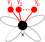
Figure 4: Graphical structure of contributions to the $n$th order coefficient $G_{p,n}(y_{1},...,y_{p})$ connected to one internal point $x$.

Now it is possible to sum all $n$ contributions in the expansion in $\varepsilon$ to form $G_{p}(\varepsilon)=\sum_{n}G_{p,n}\varepsilon^{n}$.

Case $p=1$. Evaluating (53) for $p=1$ we find that the coefficients can be expressed as

$$G_{1,n} = -\tfrac{igm^{-2}}{2^{n}n!}\big{[}\tfrac{2\Delta(0)}{\pi}\big{]}^{1/2}\lim_{N\to 0}\big{(}\tfrac{d}{dN}\big{)}^{n}$$ (54)

$$\!\!\!\!\times\leavevmode\nobreak\ \big{[}2\mu_{0}^{2-D}\Delta(0)\big{]}^{N}\sin(\pi N)\Gamma(N+2).$$

Thus, $G_{1}(\varepsilon)=\sum_{n}G_{1,n}\varepsilon^{n}$ follows immediately as

$$G_{1}(\varepsilon) = -\tfrac{igm^{-2}}{\sqrt{\pi}}\big{[}2\mu_{0}^{2-D}\Delta(0)\big{]}^{(\varepsilon+1)/2}\mu_{0}^{-1+D/2}$$

$$\quad\times\,\Gamma\big{(}2+\tfrac{\varepsilon}{2}\big{)}\sin\big{(}\tfrac{\pi\varepsilon}{2}\big{)}$$

because $G_{1,n}$ in (54) are the coefficients of a Taylor expansion about $N+\frac{\varepsilon}{2}$. [That is, the exponential of a derivative is a translation operator: $\exp\big{(}\frac{\varepsilon}{2}\frac{d}{dN}\big{)}f(N)=f\big{(}N+\frac{\varepsilon}{2}\big{)}$.]

Now, in the limit $\delta\to 0$, we get

$$G_{1}(\varepsilon)\sim-\frac{igm^{-2}}{\pi^{(\varepsilon+2)/2}}\delta^{-(\varepsilon+1)/2}\Gamma\big{(}2+\tfrac{\varepsilon}{2}\big{)}\sin\big{(}\tfrac{\pi\varepsilon}{2}\big{)}.$$

From this equation we see that in this multiple-scale approximation the summation leads to an algebraic structure for the divergence as $\delta\to 0$ that becomes more pronounced with increasing $\varepsilon$. As expected, expanding this result for small values of $\varepsilon$ gives the previously obtained result $G_{1}(\varepsilon)\to-igm^{-2}\delta^{-1/2}\varepsilon/2$ plus terms containing the same power of $\delta^{-1/2}$ multiplied by logarithms of $\delta$.

Similarly, we can evaluate $G_{2}(\varepsilon)$ in this limit. From (53) the expansion coefficients become

$$G_{2,n}=-\frac{g\mu_{0}^{2}}{2^{n-1}n!\sqrt{\pi}}\int d^{D}x\,\Delta(x-y_{1})\Delta(y_{2}-x)$$

$$\!\!\!\!\!\!\times\leavevmode\nobreak\ \lim_{N\to 0}\big{(}\tfrac{d}{dN}\big{)}^{n}(N+1)\big{[}2\mu_{0}^{2-D}\Delta(0)\big{]}^{N}\cos(\pi N)\Gamma\big{(}N+\mbox{$\textstyle{\frac{3}{2}}$}\big{)}$$

for $n\geq 1$. The closed-form solution for the connected two-point Green’s function in this approximation is then

$$G_{2}(\varepsilon) = \Delta(y_{1}-y_{2})+gm^{-2}\big{(}1-\tfrac{D}{2}\big{)}\Delta(0)$$

$$\!\!\!\!\!\!\!\!\!\!\!\!\!\!\!\!\!\!\times\leavevmode\nobreak\ \Big{[}1-\big{(}\tfrac{2+\varepsilon}{\sqrt{\pi}}\big{)}\big{[}2\mu_{0}^{2-D}\Delta(0)\big{]}^{\varepsilon/2}\cos\big{(}\mbox{$\textstyle{\frac{1}{2}}$}\pi\varepsilon\big{)}\Gamma\big{(}\tfrac{\varepsilon}{2}+\mbox{$\textstyle{\frac{3}{2}}$}\big{)}\Big{]},$$

where we have suppressed the spatial argument $(y_{1}-y_{2})$ of $G_{2}(\varepsilon)$. In the limit of small $\varepsilon$, we recover (49) to linear order and in particular in the double limit, taking $\delta\to 0$. This reconfirms the previous results, but also demonstrates that the two-point Green’s function has an algebraic $\delta$ dependence, given as

$$G_{2}(\varepsilon) = \tfrac{1}{2\pi}K_{0}(m\mu_{0}|y_{1}-y_{2}|)+\tfrac{1}{4\pi}{gm^{-2}}$$

$$\!\!\!\!\!\!\times\leavevmode\nobreak\ \Big{[}1-\tfrac{2+\varepsilon}{\sqrt{\pi}}(\pi\delta)^{-\varepsilon/2}\cos\big{(}\mbox{$\textstyle{\frac{1}{2}}$}\pi\varepsilon\big{)}\Gamma\big{(}\tfrac{\varepsilon}{2}+\mbox{$\textstyle{\frac{3}{2}}$}\big{)}\Big{]}$$

for arbitrary $\varepsilon$. As $\varepsilon$ increases, the divergence in $G_{2}(\varepsilon)$ also becomes more pronounced.

This procedure applies to higher-order Green’s functions. The summation over $n$ with coefficients $G_{p,n}$ from (53) can be performed, leading to

$$G_{p}(\varepsilon) \simeq -g\mu_{0}^{2}\frac{\Delta(0)}{\sqrt{\pi}}\Big{(}\frac{2}{\Delta(0)}\Big{)}^{p/2}\int d^{D}x\prod_{i=1}^{p}\Delta(x-y_{i})$$ (57)

$$\times \big{[}2\mu_{0}^{2-D}\Delta(0)\big{]}^{\varepsilon/2}\frac{\Gamma\big{(}\mbox{$\textstyle{\frac{1}{2}}$}\varepsilon+\mbox{$\textstyle{\frac{3}{2}}$}\big{)}\Gamma\big{(}\mbox{$\textstyle{\frac{1}{2}}$}\varepsilon+2\big{)}}{\Gamma\big{(}\mbox{$\textstyle{\frac{1}{2}}$}\varepsilon+2-\frac{p}{2}\big{)}}$$

$$\times \left\{\begin{array}[]{ll}i\sin(\pi\varepsilon/2)&p\quad{\rm odd}\\ \cos(\pi\varepsilon/2)&p\quad{\rm even}\end{array}\right.$$

in which the spatial arguments of $G_{p}(\varepsilon)$ have again been suppressed. From this, it is evident that for $p>2$

$$G_{p}(\varepsilon)\sim\delta^{p/2-1-\varepsilon/2}\quad(\delta\to 0).$$

IV Summary and outlook

The Euclidean Lagrangian $\mathcal{L}=\mbox{$\textstyle{\frac{1}{2}}$}(\nabla\phi)^{2}+\mbox{$\textstyle{\frac{1}{2}}$}\mu^{2}\phi^{2}+\mbox{$\textstyle{\frac{1}{2}}$}g\mu_{0}^{2}\phi^{2}\big{(}i\mu_{0}^{1-D/2}\phi)^{\varepsilon}$, as a field-theoretic generalization of the quantum-mechanical Lagrangian $\mathcal{L}_{qm}=\mbox{$\textstyle{\frac{1}{2}}$}(\nabla x)^{2}+\mbox{$\textstyle{\frac{1}{2}}$}x^{2}(ix)^{2}$, is a laboratory for the study of $\mathcal{PT}$-symmetric bosonic field theories. We have calculated the connected Green’s functions $G_{1}(\varepsilon)$, $G_{2}(\varepsilon;\,y_{1}-y_{2})$, and $G_{3}(\varepsilon;\,y_{1},y_{2},y_{3})$ to second order in an expansion in powers of $\varepsilon$, with an emphasis on examining the limit of this expansion as the spacetime dimension approaches 2 from below; that is as $\delta=2-D\to 0$. We have shown that divergences appear in this limit: Specifically, to first order in $\varepsilon$ the expansion coefficients in the sum $G_{p}=\sum G_{p,n}\varepsilon^{n}$ go as $G_{p,n}\sim\delta^{p/2-1}$. Thus, we observe algebraic divergences for $p=1$. To second order in $\varepsilon$, we find that the algebraic structure in $\delta$ remains intact and the only changes involve logarithmic corrections.

We have attempted a perturbative renormalization scheme in which a counterterm of the form $iv(\varepsilon)\phi$ is introduced. This introduces a shift that makes $G_{1}(\varepsilon)$ finite but evidently this does not modify the $\delta$-dependence of higher-order Green’s functions. We have demonstrated this explicitly with our calculation of $G_{2}(\varepsilon)$. On the other hand, including an explicit mass parameter $\mu_{0}$ allows for a mass renormalization, which is obtained from the two-point Green’s function $G_{2}$.

Taking a completely different approach, we have calculated $G_{p}(\varepsilon)$ to all orders in $\varepsilon$ in a leading-log expansion in the context of multiple-scale perturbation theory. In this approximation the logarithmic divergences in $\delta$ sum to yield an algebraic result.

Both results presented here, the perturbative calculation in $\varepsilon$ and the leading-logarithm sum to all powers in $\varepsilon$, can be reconciled for small values of $\varepsilon$. However, it does not yet answer the question as to why in the perturbative calculation the Green’s functions of the order $p\geq 3$ appear to vanish in the limit $\delta\to 0$. Of course, the work presented here does not imply that the full theory becomes noninteracting as $D\to 2$, but it is clear that additional work is required to develop a more robust procedural approach.

- (1) C. M. Bender and S. Boettcher, Phys. Rev. Lett. 80, 5243 (1998).
- (2) C. M. Bender, Rep. Prog. Phys. 70, 947 (2007).
- (3) C. M. Bender et al., PT Symmetry in Quantum and Classical Physics (World Scientific, Singapore, 2019).
- (4) J. Rubinstein, P. Sternberg, and Q. Ma, Phys. Rev. Lett. 99, 167003 (2007).
- (5) A. Guo, G. J. Salamo, D. Duchesne, R. Morandotti, M. Volatier-Ravat, V. Aimez, G. A. Siviloglou, and D. N. Christodoulides, Phys. Rev. Lett. 103, 093902 (2009).
- (6) C. E. Rüter, K. G. Makris, R. El-Ganainy, D. N. Christodoulides, M. Segev, and D. Kip, Nat. Phys. 6, 192-195 (2010).
- (7) K. F. Zhao, M. Schaden, and Z. Wu, Phys. Rev. A 81, 042903 (2010).
- (8) Z. Lin, H. Ramezani, T. Eichelkraut, T. Kottos, H. Cao, and D. N. Christodoulides, Phys. Rev. Lett. 106, 213901 (2011).
- (9) L. Feng, M. Ayache, J. Huang, Y.-L. Xu, M. H. Lu, Y. F. Chen, Y. Fainman, and A. Scherer, Science 333, 729 (2011).
- (10) J. Schindler, A. Li, M. C. Zheng, F. M. Ellis, and T. Kottos, Phys. Rev. A 84, 040101(R) (2011).
- (11) S. Bittner, B. Dietz, U. Günther, H. L. Harney, M. Miski-Oglu, A. Richter, and F. Schäfer, Phys. Rev. Lett. 108, 024101 (2012).
- (12) N. Chtchelkatchev, A. Golubov, T. Baturina, and V. Vinokur, Phys. Rev. Lett. 109, 150405 (2012).
- (13) C. Zheng, L. Hao, and G. L. Long, Phil. Trans. R. Soc. A 371, 20120053 (2013).
- (14) C. M. Bender, B. Berntson, D. Parker, and E. Samuel, Am. J. Phys. 81, 173 (2013).
- (15) B. Peng, Ş. K. Özdemir, F. Lei, F. Monifi, M. Gianfreda, G. L. Long, S. Fan, F. Nori, C. M. Bender, and L. Yang, Nat. Phys. 10, 394 (2014).
- (16) S. Assawaworrarit, X. Yu, and S. Fan, Nature 546, 387 (2017).
- (17) Y. Fu and H. Qin, arXiv:2002.12279.
- (18) C. M. Bender, N. Hassanpour, S. P. Klevansky, and S. Sarkar, Phys. Rev. D 98, 125003 (2018).
- (19) P. E. Dorey, C. Dunning, and R. Tateo, J. Phys. A: Math. Gen. 34, 5679 (2001).
- (20) P. E. Dorey, C. Dunning, and R. Tateo, J. Phys. A: Math. Theor. 40, R205 (2007).
- (21) C. M. Bender et al., PT symmetry in quantum and classical mechanics (World Scientific, Singapore, 2019).
- (22) C. M. Bender, D. C. Brody, and H. F. Jones, Phys. Rev. Lett. 93, 251601 (2004).
- (23) C. M. Bender, D. C. Brody, and H. F. Jones, Phys. Rev. D 70, 025001 (2004).
- (24) B. C. Harms, S. T. Jones, and C.-I Tan, Nucl. Phys. B 171, 392 (1980) and B. C. Harms, S. T. Jones, and C.-I Tan, Phys. Lett. B 91, 291 (1980).
- (25) J. L. Cardy and G. Mussardo, Phys. Lett. B 225, 275 (1989).
- (26) C. M. Bender and K. A. Milton, J. Phys. A: Math. Gen. 32, L87-L92 (1999)
- (27) T. D. Lee, Phys. Rev. 95, 1329 (1954).
- (28) C. M. Bender, S. F. Brandt, J.-H. Chen, and Q. Wang, Phys. Rev. D 71, 025014 (2005).
- (29) M. Sher, Phys. Rept. 179, 273 (1989).
- (30) C. M. Bender, D. W. Hook, N. E. Mavromatos, and S. Sarkar, J. Phys. A: Math. Theor. 49, 45LT01 (2016).
- (31) C. M. Bender and P. D. Mannheim, Phys. Rev. Lett. 100, 110402 (2008).
- (32) C. M. Bender, M. Moshe, and S. Sarkar, J. Phys. A: Math. Theor. 46, 102002 (2013).
- (33) C. M. Bender and S. Sarkar, J. Phys. A: Math. Theor. 46, 442001 (2013).
- (34) C. M. Bender, D. W. Hook, N. Mavromatos, and S. Sarkar, Phys. Rev. Lett. 113, 231605 (2014).
- (35) K. Jones-Smith and H. Mathur, Phys. Rev. A 82, 042101 (2010).
- (36) T. Ohlsson, Europhys. Lett. 113, 61001 (2016).
- (37) M. Aker et al. (KATRIN Collaboration), Phys. Rev. Lett. 123, 221802 (2019).
- (38) I. Aniceto, G. Başar, and R. Sciappa, Phys. Rep. 809, 1 (2019).
- (39) C. M. Bender, K. A. Milton, M. Moshe, S. S. Pinsky, and L. M. Simmons, Jr., Phys. Rev. Lett. 58, 2615 (1987).
- (40) C. M. Bender, K. A. Milton, M. Moshe, S. S. Pinsky, and L. M. Simmons, Jr., Phys. Rev. D 37, 1472 (1988).
- (41) C. M. Bender, K. A. Milton, S. S. Pinsky, and L. M. Simmons, Jr., J. Math. Phys. 30, 1447 (1989).
- (42) H. F. Jones and R. J. Rivers, Phys. Rev. D 75, 025023 (2007).
- (43) C. M. Bender, Rep. Prog. Phys. 70, 947-1018 (2007).
- (44) M. Sperling, D. Stöckinger and A. Voigt, JHEP 07, 132 (2013).
- (45) C. M. Bender, S. Boettcher, and P. N. Meisinger, J. Math. Phys. 40, 2201 (1999).
- (46) L. Comtet, Advanced Combinatorics: The Art of Finite and Infinite Expansions (Reidel, Dordrecht, 2010).
- (47) W. B. Gearhart and H. S. Shultz, The College Mathematics Journal Vol. 21(2), 90 (1990).
- (48) M. Mezard, G. Parisi, and M. Virasoro, Spin Glass Theory and Beyond: An Introduction to the Replica Method and its Applications (World Scientific, Singapore, 1987).
- (49) M. Abramowitz and I. A. Stegun, Handbook of Mathematical Functions (Dover, New York, 1972).
- (50) C. M. Bender and S. A. Orszag, Advanced Mathematical Methods for Scientists and Engineers (McGraw-Hill, New York, 1977), Chap. 11.
- (51) C. M. Bender and L. M. A. Bettencourt, Phys. Rev. Lett. 77, 4114 (1996).
- (52) C. M. Bender and L. M. A. Bettencourt, Phys. Rev. D 54, 7710 (1996).
- (53) H. Cheng and T. T. Wu, Phys. Rev. Lett. 24, 1456 (1970) and references therein.
- (54) L. Dolan and R. Jackiw, Phys. Rev D 9, 3320 (1974); E. Braaten and R. Pisarski, Nucl. Phys. B 337, 569 (1990).