eQE 2.0: Subsystem DFT Beyond GGA Functionals

Abstract

By adopting a divide-and-conquer strategy, subsystem-DFT (sDFT) can dramatically reduce the computational cost of large-scale electronic structure calculations. The key ingredients of sDFT are the nonadditive kinetic energy and exchange-correlation functionals which dominate it’s accuracy. Even though, semilocal nonadditive functionals find a broad range of applications, their accuracy is somewhat limited especially for those systems where achieving balance between exchange-correlation interactions on one side and nonadditive kinetic energy on the other is crucial. In eQE 2.0, we improve dramatically the accuracy of sDFT simulations by (1) implementing nonlocal nonadditive kinetic energy functionals based on the LMGP family of functionals; (2) adapting Quantum ESPRESSO’s implementation of rVV10 and vdW-DF nonlocal exchange-correlation functionals to be employed in sDFT simulations; (3) implementing “deorbitalized” meta GGA functionals (e.g., SCAN-L). We carefully assess the performance of the newly implemented tools on the S22-5 test set. eQE 2.0 delivers excellent interaction energies compared to conventional Kohn-Sham DFT and CCSD(T). The improved performance does not come at a loss of computational efficiency. We show that eQE 2.0 with nonlocal nonadditive functionals retains the same linear scaling behavior achieved in eQE 1.0 with semilocal nonadditive functionals.

PROGRAM SUMMARY
Program title: eQE
Licensing provisions: GNU
Distribution format: .tar.gz, git repository
Developer’s repository link: https://gitlab.com/Pavanello/eqe
Programming language: Fortran 90
External routines/libraries: BLACS, MPI
Operating system: Unix-like (Linux, macOS, Windows Subsystem for Linux)
Nature of problem: Solving the electronic structure of molecules and materials with subsystem density functional theory
Solution method: eQE
Additional comments: url of stable release http://eqe.rutgers.edu

1 Introduction

Kohn–Sham density functional theory (KS-DFT) [1, 2] is the most widely used approach for ab initio electronic structure simulations and has been employed for scientific discoveries across a broad range of disciplines such as chemistry, physics, and materials science. The success of KS-DFT is due to the good balance between computational cost and accuracy. However, due to its cubic scaling with respect to the number of electrons, $N_{e}$, KS-DFT calculations are limited in the system sizes they can approach.

Several alternative approaches have been proposed to access system sizes that relate to experimentally relevant microstates. Among them, we recall linear-scaling KS-DFT [3, 4, 5, 6], orbital-free DFT (OF-DFT) [7, 8, 9, 10, 11, 12, 13, 14], subsystem-DFT (sDFT) [15, 16, 17, 18, 19, 20, 21, 22], a combination of the two [23] and others [24, 25]. These approaches can achieve (quasi)-linear scaling by exploiting specific features, such as the “nearsightedness” of the electronic structure which arises in many non-conductive systems [3, 5].

sDFT adopts a divide-and-conquer strategy, whereby a system is split into smaller but interacting subsystems. In this way, the cubic scaling of conventional KS-DFT can be reduced. Linear scalability in sDFT is achieved by modeling the interactions between subsytems with pure density functionals: the nonadditive exchange-correlation (NAXC), the nonadditive kinetic energy (NAKE), and the long-range Coulomb interaction between the subsystems’ charge densities. Among them, the only available exact functional is the Coulomb interaction while the other two need to be approximated. Thus, the accuracy of sDFT is dictated by NAKE and NAXC.

In this work, we present version 2.0 of embedded Quantum ESPRESSO (eQE) [26], a code that implements sDFT based on Quantum ESPRESSO [27, 28, 29]. In the first release of eQE [26], we successfully implemented semilocal (GGA) level nonadditive functionals for both NAXC and NAKE with the following main features: (1) a scheme of parallel execution to distribute the workload across subsystems resulting in low data communication achieving high parallel efficiency, (2) ab initio molecular dynamics (AIMD), and (3) applicability to periodic systems. Many large systems currently outside KS-DFT’s realm of applicability have been successfully studied by eQE [30, 31, 32, 33, 34, 35, 36].

eQE 2.0 is capable of deploying nonlocal and meta-GGA (mGGA) XC and NAKE functionals yielding highly accurate simulations of weakly interacting subsystems. It is well known that, due to their dependence on the density and its derivative in only one point, semilocal XC functionals inherently lack the ability to capture intermediate-range and long-range dispersion interactions [37, 38, 39, 40, 41, 42, 43, 44, 45]. However, dispersion interactions play a crucial role in systems that are weakly bound and amenable to be treated by sDFT. mGGA and nonlocal XC functionals address these issues as mGGAs capture intermediate-range correlations due to their dependence on higher order derivatives of the density beyond the gradient or the kinetic energy density. Nonlocal functionals capture long-range dispersion interactions because they encode a dependency on the density on more than a single point at a time.

As mentioned, GGA NAKEs are widely used [18, 19, 16]. However, due to their inability to describe the inherent non-locality of the kinetic energy, GGAs work well only when the inter-subsystem density overlap is weak. In principle, nonlocal NAKEs have the potential to obtain more reliable results [8, 15] than GGAs. In practice, however, most of the available nonlocal functionals are not suitable to be used as NAKEs because they are optimized for bulk systems where the electron density is nonzero everywhere. Conversely, the subsystem densities in sDFT feature at least one non-periodic dimension where they decay to zero.

Recently, we have developed a new generation of nonlocal kinetic energy functionals [46, 12] and further adopted them as NAKEs [15] considerably improving the accuracy of sDFT in terms of both energy and electron density. However, the original implementation [15] is computationally very expensive compared to typical GGA NAKEs. In eQE 2.0, we implement a completely new scheme to evaluate nonlocal NAKEs that brings down the computational cost to almost GGA-level without sacrificing accuracy.

The remainder of this paper is organized as follows. A brief review of sDFT and the previous version of eQE is given in section 2. Details of the implementation of the new functionals and benchmark calculations are discussed in section 3. Finally, in section 4 we summarize this work and conclude with several potential future developments aimed to further increase the range of applicability of sDFT.

2 Brief review of sDFT and eQE

In sDFT, the system of interest is split into interacting subsystems of smaller size. Accordingly, the total electron density, $n({\mathbf{r}})$, is partitioned into subsystem contributions:

$$n(\mathbf{r})=\sum_{I}^{N_{s}}n_{I}({\mathbf{r}}),$$ (1)

where $N_{s}$ is the total number of subsystems and $n_{I}({\mathbf{r}})$ is the electron density of the subsystem $I$. In this way, the total energy functional of the system, $E_{\rm sDFT}[\{n_{I}\}]$, contains additive and nonadditive contributions encoding intra- and inter-subsystem interactions. Namely,

$$E_{\rm sDFT}[\{n_{I}\}]=\sum_{I}^{N_{s}}E_{KS}[n_{I},v_{ext}^{I}]+T_{s}^{\rm nadd}[\{n_{I}\}]+E_{\rm xc}^{\rm nadd}[\{n_{I}\}]+E_{\rm Coul}^{\rm nadd}[\{n_{I}\},\{v_{ext}^{I}\}]$$ (2)

where $v_{ext}^{I}$ is the external potential associated with subsystem $I$. The energy functional for each subsystem, $E_{KS}[n_{I},v_{ext}^{I}]$, is the same as the energy functional of typical KS-DFT with $v_{ext}^{I}$ as external potential and $n_{I}$ as electron density. $T_{s}^{\rm nadd}$, $E_{\rm xc}^{\rm nadd}$, and $E_{\rm Coul}^{\rm nadd}$ are the NAKE and NAXC energy functionals, and the nonadditive Coulomb energy, respectively. All these nonadditive energy functionals share the same definition:

$$F^{\rm nadd}[\{n_{I}\}]=F[n]-\sum_{I}^{N_{s}}F[n_{I}].$$ (3)

Among them only $E_{\rm Coul}^{\rm nadd}$ can be expressed exactly, the others need to be approximated.

Variational minimization of $E_{\rm sDFT}$ with respect to variations of the electron density of each subsystem leads to the following coupled KS-like equations,

$$\left[-\frac{1}{2}\nabla^{2}+v_{\rm KS}^{I}({\mathbf{r}})+v^{I}_{\rm emb}({\mathbf{r}})\right]\phi_{i}^{I}({\mathbf{r}})=\varepsilon^{I}_{i}\phi_{i}^{I}({\mathbf{r}}),$$ (4)

where $v_{\rm KS}^{I}$, $v_{\rm emb}^{I}$, $\phi_{i}^{I}$ are the KS–potential of the isolated subsystem, the embedding potential containing the functional derivatives of the nonadditive energy terms with respect to $n_{I}$, and the orbitals of subsystem $I$, respectively. The embedding potential can be written as follows:

$$\upsilon^{I}_{emb}({\mathbf{r}})=\sum^{N_{s}}_{J\neq I}\left[\int\frac{n_{J}({\mathbf{r}^{\prime}})}{|{\mathbf{r}}-{\mathbf{r}^{\prime}}|}d{\mathbf{r}^{\prime}}+v_{ext}^{J}({\mathbf{r}})\right]+\frac{\delta T_{\rm s}^{\text{nad}}[\{n_{I}\}]}{\delta n_{I}({\mathbf{r}})}+\frac{\delta E^{\text{nad}}_{\rm xc}[\{n_{I}\}]}{\delta n_{I}({\mathbf{r}})}.$$ (5)

The original version of eQE, implemented sDFT in the following way:

1. The construction of subsystem Hamiltonians and their diagonalizations are performed independently for each subsystem in parallel (all subsystems at the same time) and in a reduced subsystem-centered simulation cell.

2. Subsystems can be assigned a custom number of processors to optimize load balance.

3. The parallelization scheme is hierarchical designed to reduce inter-node communication.

4. An additional global DIIS layer [26, 47] to reduce the number of SCF cycles.

By adopting these steps, eQE achieved high parallel efficiency as showcased in several application works [30, 32, 33, 34]. We need to stress that the computational efficiency and accuracy of eQE is system dependent. In general, the larger the number of subsystems and the smaller their size, the better eQE performs compared to KS-DFT codes.

3 New Features and upgrades in eQE 2.0

In this section, We discuss the main features and updates of eQE since its original release in 2017 [26].

3.1 Nonlocal NAKEs

Recently, we developed fully nonlocal sDFT [15], which considerably improves on the accuracy of semilocal sDFT. However, in the original implementation, the computational cost was orders of magnitude larger than semilocal NAKEs. In this work, the issue was resolved by presenting a new implementation of nonlocal NAKE which achieves the same accuracy in the results at essentially the cost of semilocal functionals.

The typical form of a nonlocal kinetic energy functional is:

$$T_{s}[n]=\underbrace{T_{TF}[n]+T_{vW}[n]}_{T_{TV}[n]}+T_{NL}[n]$$ (6)

where, $T_{TF}[n]$, $T_{vW}[n]$, and $T_{NL}[n]$ are the Thomas-Fermi (TF) [48, 49] and von Weizsäcker (vW) [50] functionals, and lastly the nonlocal part of the functional, respectively. The nonlocal part is in practice a two-point functional defined by a double integration of the electron density at two different points in space. The interaction between two points is described by the so-called kernel, $\omega$:

$$T_{NL}[n]=\int\int n^{\alpha}({\mathbf{r}})\omega[n]({\mathbf{r}},{\mathbf{r}}^{\prime})n^{\beta}({\mathbf{r}}^{\prime})d{\mathbf{r}}d{\mathbf{r}}^{\prime}$$ (7)

where $\alpha$ and $\beta$ are positive numbers. The corresponding potential is obtained by functional derivative with respect to the density:

$$v_{T_{s}}({\mathbf{r}})=\frac{\delta T_{TV}[n]}{\delta n({\mathbf{r}})}+\frac{\delta T_{NL}[n]}{\delta n({\mathbf{r}})}=v_{TV}({\mathbf{r}})+v_{NL}({\mathbf{r}}).$$ (8)

As discussed in our previous work [15], direct implementation of this formalism for calculating the kinetic potential leads to numerical instabilities for both terms in the region of low electron density. In this region, the von Weizsäcker potential is inaccurate due to its dependence on the Laplacian of the electron density which is noisy for low density. The nonlocal part shares a similar issue. In eQE 2.0, we resolve these issues as follows.

For the $T_{TV}[n]=T_{TF}[n]+T_{vW}[n]$ term, the corresponding GGA formalism reads,

$$T_{TV}[n]=\int\tau_{TV}({\mathbf{r}})d{\mathbf{r}}\int\tau_{TF}({\mathbf{r}})F_{TV}[s]({\mathbf{r}})d{\mathbf{r}},$$ (9)

where $s$ is the dimensionless reduced density gradient, $s=\frac{1}{2(3\pi^{2})^{1/3}}\frac{|\nabla n({\mathbf{r}})|}{n^{3/4}({\mathbf{r}})}$, the enhancement factor $F_{TV}(s)=1+\frac{5}{3}s^{2}$, and $\tau_{TF}({\mathbf{r}})=\frac{3}{10}(3\pi^{2})^{\frac{2}{3}}n^{\frac{5}{3}}({\mathbf{r}})$. To eliminate the numerical inaccuracies arising at large $s$, we developed a numerically stable enhancement factor

$$F_{STV}(s)=1.0+\frac{5}{3}\left(\frac{s^{2}}{1.0+as^{2}}\right),$$ (10)

which is used in place of the original $F_{TV}[n]$, with $a=0.01$.

We choose the LMGP family of functionals [15] as the nonlocal kinetic energy functional in eQE 2.0. LMGP’s potential term, $v_{NL}({\mathbf{r}})$, can be written as follows:

$$v_{NL}({\mathbf{r}})=n^{-\nicefrac{{1}}{{6}}}({\mathbf{r}}){\mathcal{F}}^{-1}\bigg{[}\widetilde{n^{\nicefrac{{5}}{{6}}}}(\mathbf{q})\omega[n({\mathbf{r}})](q)\bigg{]}({\mathbf{r}}),$$ (11)

where $\widetilde{n^{\nicefrac{{5}}{{6}}}}(\mathbf{q})={\mathcal{F}}\big{[}n^{\nicefrac{{5}}{{6}}}({\mathbf{r}})\big{]}(\mathbf{q})$, $\omega[n({\mathbf{r}})](q)$ is the nonlocal kernel expressed in reciprocal space, ${\mathcal{F}}$ and ${\mathcal{F}}^{-1}$ represent forward and inverse Fourier transforms, respectively. There are two important details to note:

1. the nonlocal kinetic potential has a $n^{-\nicefrac{{1}}{{6}}}({\mathbf{r}})$ factor which can lead to numerical noise in the low electron density regions.

2. The kernel of LMGP is density-dependent and of spherical symmetry, e.g., $\omega[n]({\mathbf{r}},{\mathbf{r}^{\prime}})=\omega[n({\mathbf{r}})](|{\mathbf{r}}-{\mathbf{r}^{\prime}}|)$.

To eliminate issues related to point (1) above, a density weighted mix of GGA and nonlocal potentials was implemented [15]. Namely,

$$v_{T_{s}}[n](\mathbf{r})=\left(v_{NL}[n](\mathbf{r})+v_{STV}[n](\mathbf{r})\right)W[n](\mathbf{r})+v_{GGA}[n](\mathbf{r})(1-W[n](\mathbf{r}))$$ (12)

where $W[n]({\mathbf{r}})=\frac{n({\mathbf{r}})}{n_{max}}$, $n_{max}$ is the maximum value of electron density in the system and $v_{GGA}$ is the potential of a well-established GGA kinetic energy functional (we use revAPBEK [51]). The kinetic energy can be obtained by line integration [52, 15]:

$$T_{s}[n]=\int n(\mathbf{r})d\mathbf{r}\int_{0}^{1}v_{T_{s}}\left[n_{t}\right](\mathbf{r})dt,$$ (13)

where $n_{t}(\mathbf{r})=tn(\mathbf{r})$. This required using a set of 40 or more $t$ points to obtain the converged results and with that 40 or more kinetic potentials $\{v_{T_{s}}[n_{t}]({\mathbf{r}})\}$ needed to be evaluated.

To reduce the computational cost and still maintain numerical stability and accuracy, eQE 2.0 features a kinetic energy density mix where the total KEDF can be approximated as:

$$T_{s}[n] =\int\tau[n]({\mathbf{r}})d{\mathbf{r}}$$ (14)

$$=\int W[n]({\mathbf{r}})\bigg{[}\tau_{NL}[n](\mathbf{r})+\tau_{STV}[n]({\mathbf{r}})\bigg{]}+\bigg{(}1-W[n]({\mathbf{r}})\bigg{)}\tau_{GGA}[n]({\mathbf{r}})d{\mathbf{r}}$$

where $\tau[n]$, $\tau_{STV}[n]$, $\tau_{GGA}[n]$, $\tau_{NL}[n]$ are the kinetic energy density for total KEDF, $T_{STV}[n]$ and $T_{GGA}[n]$ (revAPBEk [51]), respectively. The corresponding kinetic potential is

$$v_{s}[n]({\mathbf{r}}) =\frac{\delta T_{s}[n]}{\delta n({\mathbf{r}})}=\frac{\partial W[n]}{\partial n({\mathbf{r}})}\bigg{[}\tau_{NL}[n]({\mathbf{r}})+\tau_{STV}[n]({\mathbf{r}})-\tau_{GGA}[n]({\mathbf{r}})\bigg{]}$$ (15)

$$+W[n]({\mathbf{r}})\bigg{[}v_{NL}[n]({\mathbf{r}})+v_{STV}[n]({\mathbf{r}})-v_{GGA}[n]({\mathbf{r}})\bigg{]}+v_{GGA}[n]({\mathbf{r}}).$$

where $\frac{\partial W[n]}{\partial n({\mathbf{r}})}=\frac{1}{n_{max}},\,v_{GGA}[n]({\mathbf{r}})=\frac{\partial\tau_{GGA}[n]}{\partial n({\mathbf{r}})}-\nabla\cdot\frac{\partial\tau_{GGA}[n]}{\partial\nabla n({\mathbf{r}})},\,v_{STV}[n]({\mathbf{r}})=\frac{\partial\tau_{STV}[n]}{\partial n({\mathbf{r}})}-\nabla\cdot\frac{\partial\tau_{STV}[n]}{\partial\nabla n({\mathbf{r}})}$

In practice, the above equations for both KEDF Eq. (14) and kinetic potential Eq. (15) can be further separated into three terms. Namely,

$$T_{s}[n] =E_{STV}[n]+E_{GGA}[n]+E_{NL}[n],$$ (16)

$$v_{s}[n]({\mathbf{r}}) =V_{STV}[n]({\mathbf{r}})+V_{GGA}[n]({\mathbf{r}})+V_{NL}[n]({\mathbf{r}})$$ (17)

and each part can be evaluated in the following way:

1. STV term

   $$V_{STV}[n]({\mathbf{r}}) =W[n]({\mathbf{r}})v_{STV}[n]({\mathbf{r}})+\frac{\tau_{STV}[n]({\mathbf{r}})}{n_{max}},$$ (18)

   $$E_{STV}[n] =\int W[n]({\mathbf{r}})\tau_{STV}[n]({\mathbf{r}})d{\mathbf{r}}.$$ (19)

2. GGA term

   $$V_{GGA}[n]({\mathbf{r}}) =\left[1-W[n]({\mathbf{r}})\right]v_{GGA}[n]({\mathbf{r}})-\frac{\tau_{GGA}[n]({\mathbf{r}})}{n_{max}},$$ (20)

   $$E_{GGA}[n] =\int\left[1-W[n]({\mathbf{r}})\right]\tau_{GGA}[n]({\mathbf{r}})d{\mathbf{r}}.$$ (21)

3. NL term

   $$V_{NL}[n]({\mathbf{r}})=W[n]({\mathbf{r}})v_{NL}[n]({\mathbf{r}})+\frac{\tau_{NL}[n]({\mathbf{r}})}{n_{max}}$$ (22)

   where the nonlocal kinetic density $\tau_{NL}$ needs to be approximated because the functional integration procedure in Eq. (13) is too expensive. From Eq. (11) notice that $v_{NL}[n]\sim n^{2/3}$, with $W[n]\propto n$, $\tau_{NL}$ can be approximated as $\tau_{NL}[n]({\mathbf{r}})\simeq\frac{3}{8}n({\mathbf{r}})v_{NL}[n]({\mathbf{r}})$. Thus, the nonlocal kinetic energy can be approximated as:

   $$E_{NL}[n]=\int\tau_{NL}[n]({\mathbf{r}})W[n]({\mathbf{r}})d{\mathbf{r}}.$$ (23)

In this way, each time the kinetic energy/potential is evaluated, only two GGA KEDFs and one fully nonlocal term need to be calculated, dramatically reducing the computational cost compared to the original eQE implementation.

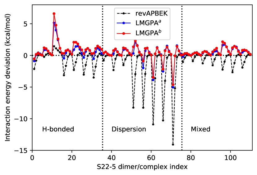
Figure 1: Interaction energy deviations against the corresponding KS-DFT results for the S22-5 test set obtained by eQE with the following NAKEs: revAPBEK (GGA), LMGPA^a (original, nonlocal), and LMGPA^b (this work, nonlocal). LMGPA is the LMGP functional with “arithmetically symmetrized” kernel as explained in [46]. PBE XC functional is adopted in all calculations. The indices on the $x$-axis correspond to complexes listed in Table S1 of the Supporting Information from Ref. [15]

The ability of nonlocal sDFT to predict interaction energies and electron densities for the S22-5 test set (noncovalently interacting complexes at equilibrium and displaced geometries[53]) has been demonstrated in our previous work [15]. To quantify the accuracy of the new implementation, we select the same test set with the same calculation settings as before. The interaction energy deviations between sDFT with different NAKEs, such as revAPBEK and LMGPA (i.e., LMGP with arithmetically symmetrized kernel [46] which we implemented in the original and new version of eQE) against the corresponding KS-DFT reference are shown in Figure 1.

The reason why we compare sDFT with KS-DFT is that in KS-DFT the total noninteracting kinetic energy is exact, while in sDFT the nonadditive part of the noninteracting kinetic energy is approximate. If the two methods deliver similar results for a given choice of exchange-correlation (we use PBE for this comparison) then it means that the approximate nonadditive functional used in sDFT is accurate. Later we will also compare against CCSD(T) benchmark values. As expected, the LMGPA nonlocal NAKE considerably improves on the results of semilocal sDFT, especially when the dimer distances are shorter than the equilibrium distance (i.e., for the S22-5(0.9) subset). Most importantly, the results from the new version of LMGPA are almost on top of the original version, showing that the new implementation maintains an excellent level of accuracy but is computationally much cheaper. A similar result is obtained when a different XC functional is used (such as a nonlocal XC functional) [15].

Hereafter, the new implementation of LMGPA (noted as LMGPA^b in the figure captions) is simply referred to as LMGPA.

3.2 Nonlocal NAXCs

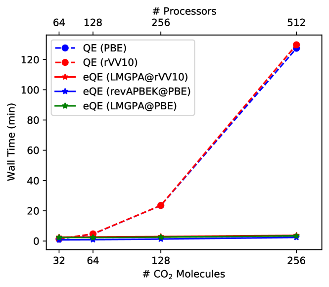
Figure 2: Wall times when simulating supercells containing 32, 64, 128, and 256 CO₂ molecules. The corresponding numbers of MPI tasks are 64, 128, 256, 512. Full lines are eQE simulations with different NAKE funtionals. Doted lines are KS-DFT (QE version 6.6) simulations for the same systems and same cutoff for the plane waves (i.e., 40 Ry for the wavefunctions and 400 Ry for the electron density).

It is well known that semilocal XC functionals struggle to describe long-range correlation effects such as dispersion interactions. However, dispersion interactions play a critically important role in a wide variety of materials, especially those composed of weakly interacting subsystems. Thus, it is necessary to adopt NAXC functionals that go beyond GGA to systematically improve the performance of sDFT.

Many nonlocal XC functionals have been proposed [54, 55, 56, 57, 58]. Among them, rVV10 [57] stands out for its accuracy across not only non-covalently bound complexes but also covalent, ionic, and metallic solids. Most importantly, the computational cost can remain low [59]. Thus, we adapted the existing rVV10 implementation of Quantum ESPRESSO [57] for eQE, where an evaluation of the functional and corresponding potential in the supersystem (physical cell) and in the subsystem-centered cells are needed. The resulting fully nonlocal sDFT compares favorably against CCSD(T) benchmark values for the interaction energies of the S22-5 set as can be seen in Figure 3.

To quantify the computational efficiency and scaling, we simulated supercells of 32, 64, 128, and 256 CO₂ molecules with the corresponding number of processors of 64, 128, 256, and 512. These calculations are performed in both KS-DFT (version 6.6 of Quantum ESPRESSO) and eQE 2.0 with both PBE and rVV10 XC functionals. Considering that the number of SCF iterations for different systems is not exactly the same, we report here the wall time for the first 20 iteration steps. As shown in Figure 2, eQE scales ideally when system size and resources are proportionally scaled. This is in contrast with version 6.6 of Quantum ESPRESSO which, as expected, scales polynomially with system size. Most importantly, The computational cost of nonlocal sDFT traces almost perfectly the scaling of semilocal sDFT. These results indicate that the implementation of nonlocal functionals for both NAKEs and NAXC are nearly ideal in eQE 2.0.

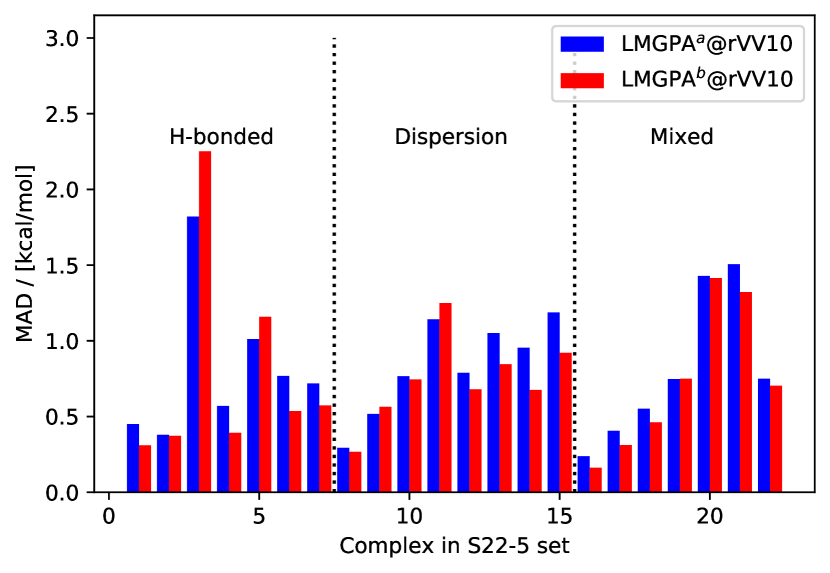
Figure 3: Interaction energy deviations against CCSD(T) benchmark values for the S22-5 test set. sDFT calculations carried out with eQE with the following NAKEs: revAPBEK (GGA), LMGPA^a (original, nonlocal), and LMGPA^b (this work, nonlocal). LMGPA is the LMGP functional with “arithmetically symmetrized” kernel as explained in [46]. rVV10 XC functional is adopted in all calculations. The indices on the $x$-axis correspond to complexes listed in Table S1 of the Supporting Information from Ref. [15]

3.3 Deorbitalized meta GGA functionals

A key challenge in DFT is the development of accurate and computationally affordable functionals for the XC energy. The so-called Perdew-Schmidt Jacob’s ladder [60, 61] provides a classification of the level of complication that goes in the formulation of the functional. The ladder leads to the “heaven of chemical accuracy”, starting from the local density approximation (LDA; dependence on $n({\mathbf{r}})$, only), generalized gradient approximations (GGA; dependent on $n({\mathbf{r}})$ and $|\nabla n({\mathbf{r}})|$), and meta-generalized gradient approximations (mGGA; dependent on $n({\mathbf{r}})$, $|\nabla n({\mathbf{r}})|$ as well as the noninteracting kinetic energy density, $\tau({\mathbf{r}})$, and possibly the density laplacian, $\nabla^{2}n({\mathbf{r}})$, and higher order derivatives). Generally, and particularly in this work, the functional dependencies of a mGGA functional can be expressed as follows

$$E_{xc}:=E_{xc}\Big{[}\xi[n,\nabla n],\tau\Big{]},$$ (24)

where the $\xi$ function represents the GGA component of the mGGA functional.

Among all functionals, GGAs dominate materials modeling mainly due to their computational efficiency and generally reliable description of various types of materials [62]. However, as mentioned, GGAs are severely limited because their description of long/intermediate-range electron-electron correlation, such as van der Waals interaction, is not satisfactory. Additionally, the presence of self-interaction [63] is detrimental for spin-polarized systems and fractional-spin systems (static correlation) [64, 65]. Among the various mGGA XC functionals, the strongly constrained and appropriately normed (SCAN) satisfies a record 17 exact conditions and can considerably improve GGAs for various systems (e.g., covalent, metallic, and even weak bonds) [66].

Unfortunately, because $\tau({\mathbf{r}})$ is typically defined in terms of the KS-DFT occupied orbitals $\{\psi_{i}\}$,

$$\tau({\mathbf{r}})=\frac{1}{2}\sum_{i=1}^{N_{e}}\left|\nabla\psi_{i}({\mathbf{r}})\right|^{2},$$ (25)

the mGGA XC potential,

$$v_{xc}({\mathbf{r}})=\frac{\delta E_{xc}\Big{[}\xi[n,\nabla n],\tau\Big{]}}{\delta n({\mathbf{r}}),}$$ (26)

cannot be directly evaluated by means of functional derivative unless expensive optimized effective potential (OEP) methods are employed [67, 68, 69].

To address this complication, a few workarounds have been proposed: (1) completely avoid the evaluation of the $\tau$-dependent mGGA potential. The mGGA functional is just used for non-self-consistent evaluation of the energy using the $n$ and $\tau$ obtained from a non-$\tau$-dependent potential [70, 71]. However, this approach is not self-consistent, i.e., the potential is not the derivative of the energy functional which can cause issues, for example, of energy conservation during an ab-initio molecular dynamics. (2) Evaluate the potential in the generalized Kohn-Sham (gKS) scheme. gKS only involves functional derivatives with respect to the KS orbitals [60, 72] (e.g., $\delta E_{xc}[\{\psi_{i}\}]/\delta\psi_{i}$) yielding an orbital-dependent XC potential. The computational cost of the gKS scheme is much cheaper than OEP, thus it is currently a widely-used approach for $\tau$-dependent mGGAs.

We note that sDFT cannot directly take advantage of the gKS scheme because only the KS orbitals of the subsystems are available. The KS orbitals of the global supersystem are never computed. This issue persists not only for mGGAs, but also for the Hartree-Fock (HF) exchange potential [73, 74].

In eQE 2.0, we decided to approach the problem from a different angle. Inspired by recent advances in the OF-DFT community, the kinetic energy density, $\tau$, can be approximated directly with a pure density functional [75, 76]. This strategy goes by the name of “deorbitalization” converting the explicit orbital-dependent mGGA XC energy functional to a pure density functional. As a result, the corresponding deorbitalized XC potential can be evaluated via Eq. (26) [76, 77].

With deorbitalization, the challenge is to approximate the kinetic energy density, not the potential or the energy. Thus, functionals that work well in OF-DFT and as nonadditive functionals in sDFT may in the end not work well for approximating the $\tau$ needed by mGGA XC functionals. GGAs might be considered, given their easy and cheap evaluation. However, many researchers [78, 79, 80] have shown that Laplacian-level functionals (i.e., those depending on $\nabla^{2}n$) are the most suitable functionals for this task.

Laplacian-level KEDF approximations can be written as follows

$$T_{s}[n,\nabla n,\nabla^{2}n]=\int\tau[n,\nabla n,\nabla^{2}n]({\mathbf{r}})d{\mathbf{r}}.$$ (27)

Thus, the deorbitalized mGGA functionals can be written as,

$$E_{xc}=\int\varepsilon_{xc}\Big{[}\xi[n,\nabla n],\tau[n,\nabla n,\nabla^{2}n]\Big{]}({\mathbf{r}})d{\mathbf{r}}=\int\varepsilon_{xc}[n,\nabla n,\nabla^{2}n]({\mathbf{r}})d{\mathbf{r}}.$$ (28)

In this way, the XC functional is an explicit density functional and the corresponding XC potential can be evaluated by Eq. (26). Namely,

$$v_{xc}=\frac{\delta E_{xc}}{\delta n}=\frac{\partial\varepsilon_{xc}}{\partial n}-\nabla\cdot(\frac{\partial\varepsilon_{xc}}{\partial\nabla n})+\nabla^{2}(\frac{\partial\varepsilon_{xc}}{\partial\nabla^{2}n}).$$ (29)

where we are omitting hereafter specific variable dependence of the density and other functions/functionals. Considering $\tau$ as a functional of $n$, $\nabla n$, and $\nabla^{2}n$ as shown in Eq. (27–28), the XC energy density partial derivatives with respect to $n$, $\nabla n$, and $\nabla^{2}n$ can be expressed as follows

$$\frac{\partial\varepsilon_{xc}}{\partial n}={\color[rgb]{1,0,0}\frac{\partial\varepsilon_{xc}}{\partial\xi}\frac{\partial\xi}{\partial n}}+{\color[rgb]{1,0,0}\frac{\partial\varepsilon_{xc}}{\partial\tau}}\frac{\partial\tau}{\partial n}$$ (30)

$$\frac{\partial\varepsilon_{xc}}{\partial\nabla n}={\color[rgb]{1,0,0}\frac{\partial\varepsilon_{xc}}{\partial\xi}\frac{\partial\xi}{\partial\nabla n}}+{\color[rgb]{1,0,0}\frac{\partial\varepsilon_{xc}}{\partial\tau}}\frac{\partial\tau}{\partial\nabla n}$$ (31)

$$\frac{\partial\varepsilon_{xc}}{\partial\nabla^{2}n}={\color[rgb]{1,0,0}\frac{\partial\varepsilon_{xc}}{\partial\tau}}\frac{\partial\tau}{\partial\nabla^{2}n}.$$ (32)

Here, the terms in red are independent of the choice of $\tau$. Thus, these operations are collected in a single subroutine for each mGGA XC functional.

To better show the formalisms of mGGA functionals related to $\tau$ parts implemented in eQE, we first define the following reduced gradient and reduced density Laplacian:

1. Reduced gradient

   $$s=\frac{|\nabla n|}{2(3\pi^{2})^{1/3}n^{4/3}}$$ (33)

   $$p=s^{2}=C_{p}\frac{|\nabla n|^{2}}{n^{8/3}}$$ (34)

2. Reduced density Laplacian

   $$q=\frac{\nabla^{2}n}{4(3\pi^{2})^{2/3}n^{5/3}}=C_{p}\frac{\nabla^{2}n}{n^{5/3}}$$ (35)

where $C_{p}=\frac{1}{4(3\pi^{2})^{2/3}}$.

In general, Laplacian-level kinetic energy density $\tau$ can be expressed as :

$$\tau=\tau_{\mathrm{TF}}F_{t}[p,q],$$ (36)

where $\tau_{\mathrm{TF}}=\frac{3}{10}(3\pi^{2})^{2/3}n^{5/3}$.

Using of Eq. (36), the kinetic energy density partial derivatives with respect to $n$, $\nabla n$, and $\nabla^{2}n$ can be further written as follows

$$\frac{\partial\tau}{\partial n}=\left({\color[rgb]{0,0,1}\frac{\partial F_{t}}{\partial p}}\frac{\partial p}{\partial n}+{\color[rgb]{0,0,1}\frac{\partial F_{t}}{\partial q}}\frac{\partial q}{\partial n}\right)\tau_{\mathrm{TF}}+\frac{\partial\tau_{TF}}{\partial n}{\color[rgb]{0,0,1}F_{t}}$$ (37)

$$\frac{\partial\tau}{\partial\nabla n}={\color[rgb]{0,0,1}\frac{\partial F_{t}}{\partial p}}\frac{\partial p}{\partial\nabla n}\tau_{\mathrm{TF}}$$ (38)

$$\frac{\partial\tau}{\partial\nabla^{2}n}={\color[rgb]{0,0,1}\frac{\partial F_{t}}{\partial q}}\frac{\partial q}{\partial\nabla^{2}n}\tau_{\mathrm{TF}},$$ (39)

where $\frac{\partial p}{\partial n}=-\frac{8}{3}p/n$, $\frac{\partial q}{\partial n}=-\frac{5}{3}q/n$, $\frac{\partial p}{\partial\nabla n}/\nabla n=\frac{2C_{p}}{n^{8/3}}$, $\frac{\partial q}{\partial\nabla^{2}n}=\frac{C_{p}}{n^{5/3}}$, and $\frac{\partial\tau_{TF}}{\partial n}=\frac{5}{3}C_{\mathrm{TF}}n^{2/3}$. The above equations (37–39) are independent of the particular mGGA XC functional used. The terms in blue color are determined only by the choice of KEDF, and the other terms are independent of the choice of both XC and KEDF. Thus, the terms in blue are evaluated in a separate, independent subroutine which is called by the subroutine that combines all terms together.

eQE 2.0 implements one of the best performing mGGA functionals, the SCAN functional [66] deorbitalized utilizing Laplacian-level KEDFs (PC [75], PCopt [76], TFLopt [76], GEA2L, L04 [78]).

3.4 A note on numerical stability

Previous works [76, 77] show that the use of the Laplacian operator can introduce noise in the results, especially when a plane-wave basis is adopted. To address this challenge we implemented a smooth Laplacian, $\hat{L_{s}}$, inspired by convolutions typically used for smoothing images. Consider $x({\mathbf{r}})$ as any physical quantity defined in real space (such as electron density $n({\mathbf{r}})$ and potential $v({\mathbf{r}})$), then, the smooth Laplacian operator, $\hat{L_{s}}$, operates on $x({\mathbf{r}})$ as,

$$\hat{L_{s}}x({\mathbf{r}})=-{\mathcal{F}}^{-1}\left[{\mathcal{F}}\left[\hat{S}\left[x({\mathbf{r}})\right]+\hat{S}\left[x({\mathbf{r}})-\hat{S}[x({\mathbf{r}})]\right]\right]|\mathbf{g}|^{2}e^{-\sigma|\mathbf{g}|^{2}}\right].$$ (40)

Where $\hat{S}$ is defined as,

$$\hat{S}x({\mathbf{r}})={\mathcal{F}}^{-1}\left[{\mathcal{F}}[x({\mathbf{r}})]e^{-\sigma|\mathbf{g}|^{2}}\right],$$ (41)

$\mathbf{g}$ is the reciprocal space vector, and $\sigma$ is a parameter. Based on our tests, $\sigma=0.02$ is a good choice to maintain numerical stability without over smoothing.

To verify the SCAN functional implemented in eQE, we implemented the subroutines we use in eQE for evaluation of SCAN functional in Quantum ESPRESSO 6.6. Our implementation of SCAN in Quantum ESPRESSO (using the gKS approach) reproduced exactly the same results as the latest version Quantum ESPRESSO with Libxc [81, 82]. This indicates that our implementation is correct. As previous work shows [78], the L04 mGGA KEDF outperforms other mGGA KEDFs when employed to approximate $\tau$ for mGGA XC functionals. Thus, here, we select L04 in all calculations. We note, however, that the PCopt KEDF has also been reported to be suitable for this task [77].

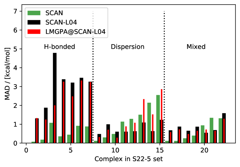
Figure 4: Mean absolute deviations (MADs) of interaction energies computed by several realizations of the SCAN functional: original (SCAN), deorbitalized SCAN with L04 KEDF for $\tau$ (SCAN-L04), and SCAN–L04 in sDFT coupled with nonlocal NAKE (LMGPA@SCAN-L04) in comparison to CCSD(T) for the S22-5 test set. The SCAN results are taken from Ref. 66. All values are given in kcal/mol. H-Bond, Dispersion and Mixed stand for hydrogen-bonded, dispersion-bonded and complexes bonded by a mix of hydrogen bonds and dispersion interactions, respectively.

Table 1: Summary of the Mean absolute deviations (MADs) of interaction energies computed with different approaches against CCSD(T) results. All values are given in kcal/mol. H-bonded, Dispersion and Mixed stand for hydrogen-bonded, dispersion-bonded and complexes bonded by a mix of hydrogen bonds and dispersion interactions, respectively.

Methods	H-bonded	Dispersion	Mixed	Total
SCAN	0.56	1.19	0.64	0.82
SCAN-L04	3.04	0.79	0.84	1.52
LMGPA@SCAN-L04	2.41	1.25	0.73	1.46

We again select the S22-5 test set with the same settings as before[15], except for the plane wave cutoffs which is increased to 500 Ry for the density and is kept to 70 Ry for the wavefunctions. As shown in Figure 4, we present the mean absolute deviations (MADs) of interaction energies obtained with different approaches in comparison to the benchmark CCSD(T) energies. These approaches include the SCAN functional implemented in the gKS scheme (SCAN), the SCAN-L04 functional (SCAN-L04), and the SCAN-L04 functional used in sDFT with the nonlocal LMGPA as NAKE (LMGPA@SCAN-L04). It is clear that SCAN-L04 delivers good interaction energies with MADs well below 5 kcal/mol. SCAN-L04 does not deteriorate the good performance of SCAN, except for the hydrogen bonded systems. Moreover, sDFT simulations with LMGPA@SCAN-L04 combination can deliver no worse results (even better for hydrogen bonded and Mixed bonded system) in comparison to SCAN-L04 results.

To further quantify the performance of SCAN-L04, we summarize the MADs of the interaction energies calculated with SCAN, SCAN-L04, and LMGPA@SCAN-L04 against CCSD(T) results in Table 1. It is clear that the performance of these three approaches are similar, since the total MAD for SCAN, SCAN-L04, and LMGPA@SCAN-L04 are 0.82, 1.52, 1.46 kcal/mol, respectively. For hydrogen-bonded systems, SCAN (0.56 kcal/mol) outperforms LMGPA@SCAN-L04 (2.41 kcal/mol) and SCAN-L04 (3.04 kcal/mol).

It is clear that deorbitalized mGGA functionals are competitive against the best pure functionals currently on the market. We envision further improvement for the deorbitalization strategy tackling the following weaknesses:

1. Deorbitalized mGGAs require larger plane-wave cutoffs to achieve converged results compared to typical GGA functionals.

2. The use of Laplacian-level KEDF for evaluating $\tau$ with plane-wave basis sets is numerically challenging. This can lead to an increase in the number of SCF iterations.

3. Currently available approximations to $\tau[n]({\mathbf{r}})$ are still fairly crude.

4 Conclusions and future directions

This work releases version 2 of embedded Quantum ESPRESSO – a code for running density embedding simulations of molecules and condensed-phase systems. Since its first release, eQE has been successfully employed for many large-scale simulations for condensed matter physics and chemistry. The new release allows the user to employ nonlocal functionals both for the kinetic energy (needed for density embedding) and exchange-correlation. Specifically, the new functionals include nonlocal nonadditive kinetic energy such as LMGPA, and nonlocal XC functionals such as rVV10. eQE version 2 also includes deorbitalized meta GGA XC functionals (i.e., where the kinetic energy density, $\tau$, is approximated by a pure density functional). Preliminary benchmark tests for the new nonlocal functionals indicate that they considerably improve on the performance of semilocal functionals in KS-DFT and subsystem DFT (embedding) calculations without increasing the computational cost significantly and, most importantly, maintaining eQE’s strong scalability with systems size.

Following this release, we will turn to further improve eQE’s performance implementing new features which may include (but not limited to) development of new nonadditive XC functionals, especially the latest SCAN variants (such as: r2SCAN [83, 84], r2SCAN+ [85, 86], SCAN+rVV10 [87]). We will also continue to develop more accurate KEDFs for both nonadditive functionals for embedding and for approximating the kinetic energy density used in deorbitalized meta GGA functionals.

5 Acknowledgments

This material is based upon work supported by the National Science Foundation under Grants No. CHE-1553993 and OAC-1931473. We thank the Office of Advanced Research Computing at Rutgers for providing access to the Amarel and Caliburn clusters.

References

- [1] P. Hohenberg, W. Kohn, Inhomogeneous Electron Gas, Phys. Rev. 136 (1964) 864–871.
- [2] W. Kohn, L. J. Sham, Self-Consistent Equations Including Exchange and Correlation Effects, Phys. Rev. 140 (1965) 1133–1138.
- [3] S. Goedecker, Linear scaling electronic structure methods, Reviews of Modern Physics 71 (4) (1999) 1085.
- [4] D. R. Bowler, T. Miyazaki, Methods in Electronic Structure Calculations, Rep. Prog. Phys. 75 (2012) 036503.
-
[5]
K.-H. Liou, C. Yang, J. R. Chelikowsky,
Scalable implementation of
polynomial filtering for density functional theory calculation in PARSEC,
Computer Physics Communications 254 (2020) 107330.
doi:10.1016/j.cpc.2020.107330.
URL https://doi.org/10.1016/j.cpc.2020.107330 -
[6]
A. M. P. Sena, T. Miyazaki, D. R. Bowler,
Linear Scaling Constrained
Density Functional Theory in CONQUEST, J. Chem. Theory Comput. 7 (2011)
884–889.
doi:10.1021/ct100601n.
URL http://dx.doi.org/10.1021/ct100601n - [7] Y. A. Wang, E. A. Carter, Orbital-Free Kinetic-Energy Density Functional Theory, in: S. D. Schwartz (Ed.), Theoretical Methods in Condensed Phase Chemistry, Kluwer, Dordrecht, 2000, pp. 117–184.
- [8] W. C. Witt, G. Beatriz, J. M. Dieterich, E. A. Carter, Orbital-free density functional theory for materials research, J. M. Res. 33 (7) (2018) 777–795.
- [9] W. Mi, X. Shao, C. Su, Y. Zhou, S. Zhang, Q. Li, H. Wang, L. Zhang, M. Miao, Y. Wang, Y. Ma, Atlas: A real-space finite-difference implementation of orbital-free density functional theory, Comput. Phys. Commun. 200 (2016) 87 – 95.
- [10] X. Shao, Q. Xu, S. Wang, J. Lv, Y. Wang, Y. Ma, Large-scale ab initio simulations for periodic system, Comput. Phys. Commun. 233 (2018) 78–83.
- [11] C. Huang, E. A. Carter, Nonlocal orbital-free kinetic energy density functional for semiconductors, Phys. Rev. B 81 (2010) 045206.
- [12] W. Mi, M. Pavanello, Orbital-free dft correctly models quantum dots when asymptotics, nonlocality and nonhomogeneity are accounted for, Phys. Rev. B Rapid Commun. 100 (2019) 041105.
- [13] K. Luo, V. V. Karasiev, S. Trickey, A simple generalized gradient approximation for the noninteracting kinetic energy density functional, Phys. Rev. B 98 (4) (2018) 041111.
- [14] V. V. Karasiev, S. B. Trickey, Issues and challenges in orbital-free density functional calculations, Comput. Phys. Commun. 183 (12) (2012) 2519–2527.
-
[15]
W. Mi, M. Pavanello,
Nonlocal subsystem density
functional theory, The Journal of Physical Chemistry Letters 11 (1) (2020)
272–279.
doi:10.1021/acs.jpclett.9b03281.
URL https://doi.org/10.1021/acs.jpclett.9b03281 -
[16]
T. A. Wesolowski, S. Shedge, X. Zhou,
Frozen-Density Embedding Strategy
for Multilevel Simulations of Electronic Structure, Chem. Rev. 115 (2015)
5891–5928.
doi:10.1021/cr500502v.
URL http://dx.doi.org/10.1021/cr500502v - [17] A. S. P. Gomes, C. R. Jacob, Quantum-chemical embedding methods for treating local electronic excitations in complex chemical systems, Annu. Rep. Prog. Chem., Sect. C: Phys. Chem. 108 (2012) 222–277.
-
[18]
C. R. Jacob, J. Neugebauer,
Subsystem density-functional
theory, WIREs: Comput. Mol. Sci. 4 (2014) 325–362.
doi:10.1002/wcms.1175.
URL http://dx.doi.org/10.1002/wcms.1175 -
[19]
A. Krishtal, D. Sinha, A. Genova, M. Pavanello,
Subsystem
Density-Functional Theory as an Effective Tool for Modeling Ground and
Excited States, their Dynamics, and Many-Body Interactions, J. Phys.:
Condens. Matter 27 (2015) 183202.
URL http://iopscience.iop.org/0953-8984/27/18/183202 -
[20]
J. Nafziger, A. Wasserman,
Density-Based Partitioning
Methods for Ground-State Molecular Calculations, J. Phys. Chem. A 118
(2014) 7623–7639.
arXiv:http://dx.doi.org/10.1021/jp504058s, doi:10.1021/jp504058s.
URL http://dx.doi.org/10.1021/jp504058s - [21] G. Senatore, K. Subbaswamy, Density dependence of the dielectric constant of rare-gas crystals, Phys. Rev. B 34 (8) (1986) 5754.
- [22] T. A. Wesolowski, A. Warshel, Frozen Density Functional Approach for ab Initio Calculations of Solvated Molecules, J. Chem. Phys. 97 (1993) 8050.
-
[23]
S. Andermatt, J. Cha, F. Schiffmann, J. VandeVondele,
Combining Linear-Scaling
DFT with Subsystem DFT in Born–Oppenheimer and Ehrenfest
Molecular Dynamics Simulations: From Molecules to a Virus in Solution, J.
Chem. Theory Comput. 12 (2016) 3214–3227.
URL http://dx.doi.org/10.1021/acs.jctc.6b00398 - [24] D. Porezag, T. Frauenheim, T. Köhler, G. Seifert, R. Kaschner, Construction of tight-binding-like potentials on the basis of density-functional theory: Application to carbon, Physical Review B 51 (19) (1995) 12947.
- [25] M. Elstner, D. Porezag, G. Jungnickel, J. Elsner, M. Haugk, T. Frauenheim, S. Suhai, G. Seifert, Self-consistent-charge density-functional tight-binding method for simulations of complex materials properties, Physical Review B 58 (11) (1998) 7260.
- [26] A. Genova, D. Ceresoli, A. Krishtal, O. Andreussi, R. DiStasio Jr., M. Pavanello, eQE — A Densitiy Functional Embedding Theory Code For The Condensed Phase, Int. J. Quantum Chem. 117 (2017) e25401. doi:10.1002/qua.25401.
-
[27]
P. Giannozzi, S. Baroni, N. Bonini, M. Calandra, R. Car, C. Cavazzoni,
D. Ceresoli, G. L. Chiarotti, M. Cococcioni, I. Dabo, A. Dal Corso,
S. de Gironcoli, S. Fabris, G. Fratesi, R. Gebauer, U. Gerstmann,
C. Gougoussis, A. Kokalj, M. Lazzeri, L. Martin-Samos, N. Marzari, F. Mauri,
R. Mazzarello, S. Paolini, A. Pasquarello, L. Paulatto, C. Sbraccia,
S. Scandolo, G. Sclauzero, A. P. Seitsonen, A. Smogunov, P. Umari, R. M.
Wentzcovitch, QUANTUM ESPRESSO: a
modular and open-source software project for quantum simulations of
materials, J. Phys.: Cond. Mat. 21 (2009) 395502.
URL http://www.quantum-espresso.org - [28] P. Giannozzi, O. Baseggio, P. Bonfà, D. Brunato, R. Car, I. Carnimeo, C. Cavazzoni, S. De Gironcoli, P. Delugas, F. Ferrari Ruffino, et al., Quantum espresso toward the exascale, J. Chem. Phys. 152 (15) (2020) 154105.
-
[29]
P. Giannozzi, O. Andreussi, T. Brumme, O. Bunau, M. B. Nardelli, M. Calandra,
R. Car, C. Cavazzoni, D. Ceresoli, M. Cococcioni, N. Colonna, I. Carnimeo,
A. D. Corso, S. de Gironcoli, P. Delugas, R. A. D. Jr, A. Ferretti,
A. Floris, G. Fratesi, G. Fugallo, R. Gebauer, U. Gerstmann, F. Giustino,
T. Gorni, J. Jia, M. Kawamura, H.-Y. Ko, A. Kokalj, E. Küçükbenli,
M. Lazzeri, M. Marsili, N. Marzari, F. Mauri, N. L. Nguyen, H.-V. Nguyen,
A. O. de-la Roza, L. Paulatto, S. Poncé, D. Rocca, R. Sabatini, B. Santra,
M. Schlipf, A. P. Seitsonen, A. Smogunov, I. Timrov, T. Thonhauser, P. Umari,
N. Vast, X. Wu, S. Baroni,
Advanced capabilities
for materials modelling with q uantum espresso, Journal of Physics:
Condensed Matter 29 (46) (2017) 465901.
URL http://stacks.iop.org/0953-8984/29/i=46/a=465901 -
[30]
A. Umerbekova, M. Pavanello,
Many-body response of benzene at
monolayer MoS2: Van der Waals interactions and spectral broadening,
International Journal of Quantum Chemistry (2020) e26243doi:10.1002/qua.26243.
URL https://doi.org/10.1002/qua.26243 -
[31]
A. Umerbekova, S.-F. Zhang, S. K. P., M. Pavanello,
Dissecting energy level
renormalization and polarizability enhancement of molecules at surfaces with
subsystem TDDFT, Eur. Phys. J. B 91 (2018).
doi:10.1140/epjb/e2018-90145-2.
URL https://doi.org/10.1140/epjb/e2018-90145-2 -
[32]
S. K. P., A. Genova, M. Pavanello,
Cooperation and
environment characterize the low-lying optical spectrum of liquid water, J.
Phys. Chem. Lett. 8 (2017) 5077–5083.
doi:10.1021/acs.jpclett.7b02212.
URL https://doi.org/10.1021/acs.jpclett.7b02212 -
[33]
W. Mi, P. Ramos, J. Maranhao, M. Pavanello,
Ab initio structure and
dynamics of CO2 at supercritical conditions, J. Phys. Chem. Lett.
10 (24) (2019) 7554–7559.
doi:10.1021/acs.jpclett.9b03054.
URL https://doi.org/10.1021/acs.jpclett.9b03054 -
[34]
A. Genova, D. Ceresoli, M. Pavanello,
Avoiding
Fractional Electrons in Subsystem DFT Based Ab-Initio Molecular Dynamics
Yields Accurate Models For Liquid Water and Solvated OH Radical, J. Chem.
Phys. 144 (2016) 234105.
doi:10.1063/1.4953363.
URL http://scitation.aip.org/content/aip/journal/jcp/144/23/10.1063/1.4953363 -
[35]
A. Genova, D. Ceresoli, M. Pavanello,
Periodic Subsystem Density-Functional
Theory, J. Chem. Phys. 141 (2014) 174101.
doi:10.1063/1.4897559.
URL http://arxiv.org/abs/1406.7803 - [36] A. Genova, M. Pavanello, Exploiting the Locality of Subsystem Density Functional Theory: Efficient Sampling of the Brillouin Zone, J. Phys.: Condens. Matter 27 (2015) 495501. doi:10.1088/0953-8984/27/49/495501.
- [37] A. J. Misquitta, B. Jeziorski, K. Szalewicz, Dispersion Energy from Density-Functional Theory Description of Monomers, Phys. Rev. Lett. 91 (2003) 033201.
-
[38]
K. Pernal, R. Podeszwa, K. Patkowski, K. Szalewicz,
Dispersionless
Density Functional Theory, Phys. Rev. Lett. 103 (2009) 263201.
doi:10.1103/PhysRevLett.103.263201.
URL http://link.aps.org/doi/10.1103/PhysRevLett.103.263201 -
[39]
J. Klimes, D. R. Bowler, A. Michaelides,
Chemical accuracy for
the van der Waals density functional, J. Phys.: Condens. Matter 22 (2010)
022201.
URL http://stacks.iop.org/0953-8984/22/i=2/a=022201 -
[40]
J. Klimeš, A. Michaelides,
Perspective: Advances and
challenges in treating van der Waals dispersion forces in density functional
theory, J. Chem. Phys. 137 (2012) 120901.
doi:10.1063/1.4754130.
URL http://link.aip.org/link/?JCP/137/120901/1 -
[41]
O. A. Vydrov, T. Van Voorhis,
Benchmark Assessment of
the Accuracy of Several van der Waals Density Functionals, J. Chem. Theory
Comput. 8 (2012) 1929–1934.
arXiv:http://pubs.acs.org/doi/pdf/10.1021/ct300081y, doi:10.1021/ct300081y.
URL http://pubs.acs.org/doi/abs/10.1021/ct300081y -
[42]
D. C. Langreth, M. Dion, H. Rydberg, E. Schröder, P. Hyldgaard, B. I.
Lundqvist, Van der Waals density
functional theory with applications, Int. J. Quantum Chem. 101 (2005)
599–610.
doi:10.1002/qua.20315.
URL http://dx.doi.org/10.1002/qua.20315 - [43] J. F. Dobson, T. Gould, Calculation of dispersion energies, J. Phys.: Condens. Matter 24 (2012) 073201.
- [44] N. Ferri, R. A. DiStasio, A. Ambrosetti, R. Car, A. Tkatchenko, Electronic Properties of Molecules and Surfaces with a Self-Consistent Interatomic van der Waals Density Functional, Phys. Rev. Lett. 114 (17) (apr 2015).
- [45] J. Hermann, R. A. DiStasio, A. Tkatchenko, First-principles models for van der waals interactions in molecules and materials: Concepts, theory, and applications, Chem. Rev. 117 (2017) 4714–4758. doi:10.1021/acs.chemrev.6b00446.
- [46] W. Mi, A. Genova, M. Pavanello, Nonlocal kinetic energy functionals by functional integration 148 (18) (2018) 184107.
- [47] P. Pulay, Improved SCF Convergence Acceleration, J. Comput. Chem. 3 (1982) 556–560.
- [48] E. Fermi, Un Metodo Statistico per la Determinazione di alcune Prioprietà dell’Atomo, Rend. Accad. Naz. Lincei 6 (1927) 602–607.
- [49] L. A. Thomas, The calculation of atomic fields, Proc. Camb. Phil. Soc. 23 (1927) 542–548.
- [50] C. F. von Weizsäcker, Zur Theorie der Kernmassen, Z. Physik 96 (1935) 431–458.
- [51] L. A. Constantin, E. Fabiano, S. Laricchia, F. Della Sala, Semiclassical neutral atom as a reference system in density functional theory, Phys. Rev. Lett. 106 (18) (2011) 186406.
-
[52]
J.-D. Chai, J. D. Weeks,
Orbital-free
density functional theory: Kinetic potentials and ab initio local
pseudopotentials, Phys. Rev. B 75 (2007) 205122.
doi:10.1103/PhysRevB.75.205122.
URL http://link.aps.org/doi/10.1103/PhysRevB.75.205122 -
[53]
L. Grafova, M. Pitonak, J. Rezac, P. Hobza,
Comparative Study of Selected Wave
Function and Density Functional Methods for Noncovalent Interaction Energy
Calculations Using the Extended S22 Data Set, J. Chem. Theory Comput. 6
(2010) 2365–2376.
doi:10.1021/ct1002253.
URL https://doi.org/10.1021/ct1002253 - [54] M. Dion, H. Rydberg, E. Schröder, D. C. Langreth, B. I. Lundqvist, Van der waals density functional for general geometries, Phys. Rev. Lett. 92 (24) (2004) 246401.
- [55] K. Lee, É. D. Murray, L. Kong, B. I. Lundqvist, D. C. Langreth, Higher-accuracy van der waals density functional, Physical Review B 82 (8) (2010) 081101.
- [56] O. A. Vydrov, T. Van Voorhis, Nonlocal van der waals density functional made simple, Phys. Rev. Lett. 103 (6) (2009) 063004.
- [57] R. Sabatini, T. Gorni, S. De Gironcoli, Nonlocal van der waals density functional made simple and efficient, Phys. Rev. B 87 (4) (2013) 041108.
- [58] O. A. Vydrov, T. Van Voorhis, Nonlocal van der waals density functional: The simpler the better, J. Chem. Phys. 133 (24) (2010) 244103.
-
[59]
G. Román-Pérez, J. M. Soler,
Efficient
Implementation of a van der Waals Density Functional: Application to
Double-Wall Carbon Nanotubes, Phys. Rev. Lett. 103 (2009) 096102.
doi:10.1103/PhysRevLett.103.096102.
URL http://link.aps.org/doi/10.1103/PhysRevLett.103.096102 -
[60]
J. Tao, J. P. Perdew, V. N. Staroverov, G. E. Scuseria,
Climbing the
density functional ladder: Nonempirical meta–generalized gradient
approximation designed for molecules and solids, Phys. Rev. Lett. 91 (2003)
146401.
doi:10.1103/PhysRevLett.91.146401.
URL https://link.aps.org/doi/10.1103/PhysRevLett.91.146401 -
[61]
J. P. Perdew, Jacob’s ladder of
density functional approximations for the exchange-correlation energy, in:
AIP Conference Proceedings, AIP, 2001.
doi:10.1063/1.1390175.
URL https://doi.org/10.1063%2F1.1390175 -
[62]
M. G. Medvedev, I. S. Bushmarinov, J. Sun, J. P. Perdew, K. A. Lyssenko,
Density functional theory is
straying from the path toward the exact functional, Science 355 (6320)
(2017) 49–52.
doi:10.1126/science.aah5975.
URL https://doi.org/10.1126/science.aah5975 - [63] J. P. Perdew, A. Zunger, Self-Interaction Correction To Density-Functional Approximations For Many-Electron Systems, Phys. Rev. B 23 (1981) 5048.
- [64] A. J. Cohen, P. Mori-Sanchez, W. Yang, Challenges for Density Functional Theory, Chem. Rev. 112 (2011) 289–318.
- [65] A. J. Cohen, P. Mori-Sanchez, W. Yang, Insights into Current Limitations of Density Functional Theory, Science 321 (2008) 792–794. doi:10.1126/science.1158722.
-
[66]
J. Sun, A. Ruzsinszky, J. P. Perdew,
Strongly constrained
and appropriately normed semilocal density functional, Phys. Rev. Lett.
115 (3) (2015).
doi:10.1103/physrevlett.115.036402.
URL https://doi.org/10.1103/physrevlett.115.036402 -
[67]
W. Yang, Q. Wu, Direct
method for optimized effective potentials in density-functional theory,
Physical Review Letters 89 (14) (sep 2002).
doi:10.1103/physrevlett.89.143002.
URL https://doi.org/10.1103/physrevlett.89.143002 -
[68]
A. Görling, Orbital- and
state-dependent functionals in density-functional theory, J. Chem. Phys.
123 (2005) 062203.
doi:10.1063/1.1904583.
URL http://link.aip.org/link/?JCP/123/062203/1 - [69] A. V. Arbuznikov, M. Kaupp, The self-consistent implementation of exchange-correlation functionals depending on the local kinetic energy density, Chemical physics letters 381 (3-4) (2003) 495–504.
- [70] J. P. Perdew, S. Kurth, A. Zupan, P. Blaha, Accurate density functional with correct formal properties: A step beyond the generalized gradient approximation, Phys. Rev. Lett. 82 (12) (1999) 2544.
- [71] M. Ernzerhof, G. E. Scuseria, Kinetic energy density dependent approximations to the exchange energy, J. Chem. Phys. 111 (3) (1999) 911–915.
- [72] J. C. Womack, N. Mardirossian, M. Head-Gordon, C.-K. Skylaris, Self-consistent implementation of meta-gga functionals for the onetep linear-scaling electronic structure package, J. Chem. Phys. 145 (20) (2016) 204114.
-
[73]
S. Laricchia, E. Fabiano, F. Della Sala,
Frozen density embedding
with hybrid functionals, J. Chem. Phys. 133 (2010) 164111.
doi:10.1063/1.3494537.
URL http://link.aip.org/link/?JCP/133/164111/1 -
[74]
S. Laricchia, E. Fabiano, F. Della Sala,
On the Accuracy of Frozen
Density Embedding Calculations with Hybrid and Orbital-Dependent Functionals
for Non-Bonded Interaction Energies, J. Chem. Phys. 137 (1) (2012) 014102.
doi:10.1063/1.4730748.
URL http://link.aip.org/link/?JCP/137/014102/1 - [75] J. P. Perdew, L. A. Constantin, Laplacian-level density functionals for the kinetic energy density and exchange-correlation energy, Physical Review B 75 (15) (2007) 155109.
- [76] D. Mejia-Rodriguez, S. Trickey, Deorbitalization strategies for meta-generalized-gradient-approximation exchange-correlation functionals, Physical Review A 96 (5) (2017) 052512.
- [77] D. Mejia-Rodriguez, S. Trickey, Deorbitalized meta-gga exchange-correlation functionals in solids, Physical Review B 98 (11) (2018) 115161.
- [78] S. Laricchia, L. A. Constantin, E. Fabiano, F. Della Sala, Laplacian-Level Kinetic Energy Approximations Based on the Fourth-Order Gradient Expansion: Global Assessment and Application to the Subsystem Formulation of Density Functional Theory, J. Chem. Theory Comput. 10 (1) (2014) 164–179.
-
[79]
S. Smiga, E. Fabiano, L. A. Constantin, F. D. Sala,
Laplacian-dependent models of the
kinetic energy density: Applications in subsystem density functional theory
with meta-generalized gradient approximation functionals, J. Chem. Phys.
146 (6) (2017) 064105.
doi:10.1063/1.4975092.
URL https://doi.org/10.1063/1.4975092 -
[80]
S. Laricchia, L. A. Constantin, E. Fabiano, F. D. Sala,
Laplacian-level kinetic energy
approximations based on the fourth-order gradient expansion: Global
assessment and application to the subsystem formulation of density functional
theory, ”J. Chem. Theory Comput.” 10 (2013) 164–179.
doi:10.1021/ct400836s.
URL https://doi.org/10.1021/ct400836s - [81] S. Lehtola, C. Steigemann, M. J. Oliveira, M. A. Marques, Recent developments in libxc–a comprehensive library of functionals for density functional theory, SoftwareX 7 (2018) 1–5.
- [82] M. A. Marques, M. J. Oliveira, T. Burnus, Libxc: A library of exchange and correlation functionals for density functional theory, Computer physics communications 183 (10) (2012) 2272–2281.
- [83] J. W. Furness, A. D. Kaplan, J. Ning, J. P. Perdew, J. Sun, Accurate and numerically efficient r2scan meta-generalized gradient approximation, The journal of physical chemistry letters 11 (19) (2020) 8208–8215.
- [84] D. Mejía-Rodríguez, S. Trickey, Meta-gga performance in solids at almost gga cost, Physical Review B 102 (12) (2020) 121109.
- [85] S. Ehlert, U. Huniar, J. Ning, J. W. Furness, J. Sun, A. D. Kaplan, J. P. Perdew, J. G. Brandenburg, r2scan-d4: Dispersion corrected meta-generalized gradient approximation for general chemical applications, arXiv preprint arXiv:2012.09249 (2020).
- [86] S. Grimme, A. Hansen, S. Ehlert, J.-M. Mewes, r2scan-3c: An efficient ”swiss army knife” composite electronic-structure method (2020).
- [87] H. Peng, Z.-H. Yang, J. P. Perdew, J. Sun, Versatile van der waals density functional based on a meta-generalized gradient approximation, Physical Review X 6 (4) (2016) 041005.