A resampling approach for causal inference on novel two-point time-series with application to identify risk factors for type-2 diabetes and cardiovascular disease

Abstract

[Abstract] Two-point time-series data, characterized by baseline and follow-up observations, are frequently encountered in health research. We study a novel two-point time-series structure without a control group, which is driven by an observational routine clinical dataset collected to monitor key risk markers of type-$2$ diabetes (T2D) and cardiovascular disease (CVD). We propose a resampling approach called ‘I-Rand’ for independently sampling one of the two time points for each individual and making inference on the estimated causal effects based on matching methods. The proposed method is illustrated with data from a service-based dietary intervention to promote a low-carbohydrate diet (LCD), designed to impact risk of T2D and CVD. Baseline data contain a pre-intervention health record of study participants, and health data after LCD intervention are recorded at the follow-up visit, providing a two-point time-series pattern without a parallel control group. Using this approach we find that obesity is a significant risk factor of T2D and CVD, and an LCD approach can significantly mitigate the risks of T2D and CVD. We provide code that implements our method.

1 Introduction

Cardiovascular disease (CVD) including stroke and coronary heart diseases, has become the most common non-communicable disease in the United States, and is also a severe problem globally ^{1, 2}. Type-2 diabetes (T2D) doubles the risk of CVD, which is the principal cause of death in T2D patients ³. CVD and T2D produce an immense economic burden on health care systems globally. Targeted intervention for individuals at increased risk of CVD and T2D plays a crucial role in reducing the global burden of these diseases⁴. Consequently, the identification of dietary and lifestyle risk factors for T2D and CVD has become a health priority ⁵. Since obesity is a substantial contributor to T2D, and consequently to the risk of CVD, ⁶ lowering obesity through diet control may help to alleviate the T2D and CVD epidemics.

In this work, we pursue two scientific goals. First, we seek to determine whether or not obesity is a significant risk factor for T2D and CVD. Second we ask if a low-carbohydrate diet (LCD) improves on standard care for T2D and CVD risk in patients with prediabetes or diabetes. We use causal inference tools, including the potential outcome model and mediation analysis, to quantify the impact of obesity and diet on T2D and CVD risk. To explore the link between obesity and T2D, we ask: what would the effect on T2D be if an individual were to change from a normal weight to an obese weight? Motivated by the impact of T2D in CVD risk, we seek to understand the role of T2D in mediating the effect of obesity on CVD risk. This mediation analysis is relevant to an individual with limited control over his or her T2D status and who wishes to identify factors that can be controlled. We perform mediation analysis to identify obesity as a significant risk factor for T2D and CVD and to disentangle cause-and-effect relationships in individuals with both conditions. Building on these questions, we are also interested in quantifying the effects of an LCD, which restricts the consumption of carbohydrates relative to the average diet⁷, on both T2D and CVD risk. Several systematic reviews and meta-analyses of randomized control trials suggest beneficial effects of LCD in T2D and CVD ^{8, 9, 10}. However, the impact of LCD in a primary care setting with observational data and its cause-and-effect inferences has not been thoroughly evaluated ^{2, 11, 12}. As we discuss in detail later in this article, our results indicate that obesity is a significant risk factor for T2D and CVD, and that LCD can significantly lower the risks of T2D and CVD risk.

We explore our scientific questions by analyzing clinical data from patients who visited a health clinic in the UK on two occasions. These patients began a low-carbohydrate diet subsequent to the first visit, and standard measurements of their health were taken at both visits. Data on these patients naturally comprise a panel dataset with two time points. In this two-point time-series dataset, there is no control group, which poses a challenge for causal inference. We propose a novel approach to dealing with this challenge, “I-Rand," which estimates average treatment effect and its significance on a collection of sub-samples of our dataset. Each subsample contains exactly one of the two observations corresponding to each individual. The average treatment effect within each subsample relies on propensity score matching, and statistical significance is estimated with a permutation test. Such subsampling has been used previously by Hahn ¹³ in the analysis of spatial point patterns. We benchmark I-Rand against two alternative estimation methods. The I-Rand algorithm meets the Stable Unit Treatment Value Assumption (SUTVA) of “no-interference” for valid causal inference, unlike the pooled approach^{14, 15}. On the other hand, I-Rand permits a nonparametric estimation of treatment effect and hence is robust to the model specification as compared with difference-in-differences method^{16, 17}. Moreover, I-Rand enables us to draw inference on the significance of the estimated average treatment effect. We demonstrate through simulations that the I-Rand algorithm reduces error in estimates of the treatment effect compared to the pooled approach and difference-in-differences.

The article is organized as follows. Section 2 introduces basic concepts from the potential outcomes model and matching methods, and propose the new I-Rand algorithm that we use to analyze the two-point time-series data. Section 3 compares the proposed I-Rand with benchmark methods such as the pooled approach and the difference-in-differences. Section 4 explains the use of I-Rand to understand the role of the LCD in reducing the risks of T2D and CVD risk. Section 5 investigates the relationship between obesity, T2D, and CVD risk. We discuss the limitations of our methods and indicate directions for future research in Section 6.

2 Motivation, Dataset, and Methodology

2.1 A motivating example

Cause-and-effect questions arise naturally in the context of nutrition or health, making causal analysis especially relevant. Consider the counterfactual question, If an individual changes from a regular diet to an LCD, would he / she be less likely to develop T2D? We can attempt to estimate the effect of diet on T2D from observational data. Any cause-and-effect inferences from observational data rely on restrictive assumptions and a specification of the underlying causal structure. In particular, we make the following assumptions. First, the treatment is a binary variable that indicates whether or not an individual follows an LCD. The binary treatment LCD abstracts away the degree of LCD as this data there is clinical consultation Second, body mass index (BMI) is a surrogate for obesity and mediates the effect of LCD on T2D ¹⁸. Gender is a binary variable and age is an ordinal variable. Finally, the medical outcome T2D is an ordinal variable indicating status at time of reporting: non-diabetics, pre-diabetics, and diabetics. T2D categories rely on glycated haemoglobin (HbA1c) value. We also note that the BMI, age and gender variables reflect only the case demographics, i.e., the BMI, age and gender distributions among the tested individuals, and not the general demographics. We assume the coarse-grained causal graph in Figure 1, and motivate it by thinking of the following data-generating process: (1) LCD affects both BMI and the risk of T2D based on established knowledge of causal effects in nutrition studies ^{7, 19, 20}; (2) Gender and age affect BMI and the risk of T2D, but not the treatment LCD; (3) Conditional on the status of LCD, BMI, gender and age, T2D status is sampled as the medical outcome; (4) There are no hidden confounders (i.e., causal sufficiency). We discuss the role of unobserved variables in Section 6. We use arrows from one variable to another in the causal graph in Figure 1 (and all other causal graphs) to indicate causal relationships. Under these assumptions, we can estimate the effect of LCD on T2D by adjusting for the confounders using the model of potential outcomes.

Figure 1: Assumed coarse-grained causal graph for the relationship between LCD, BMI, and the outcome T2D.

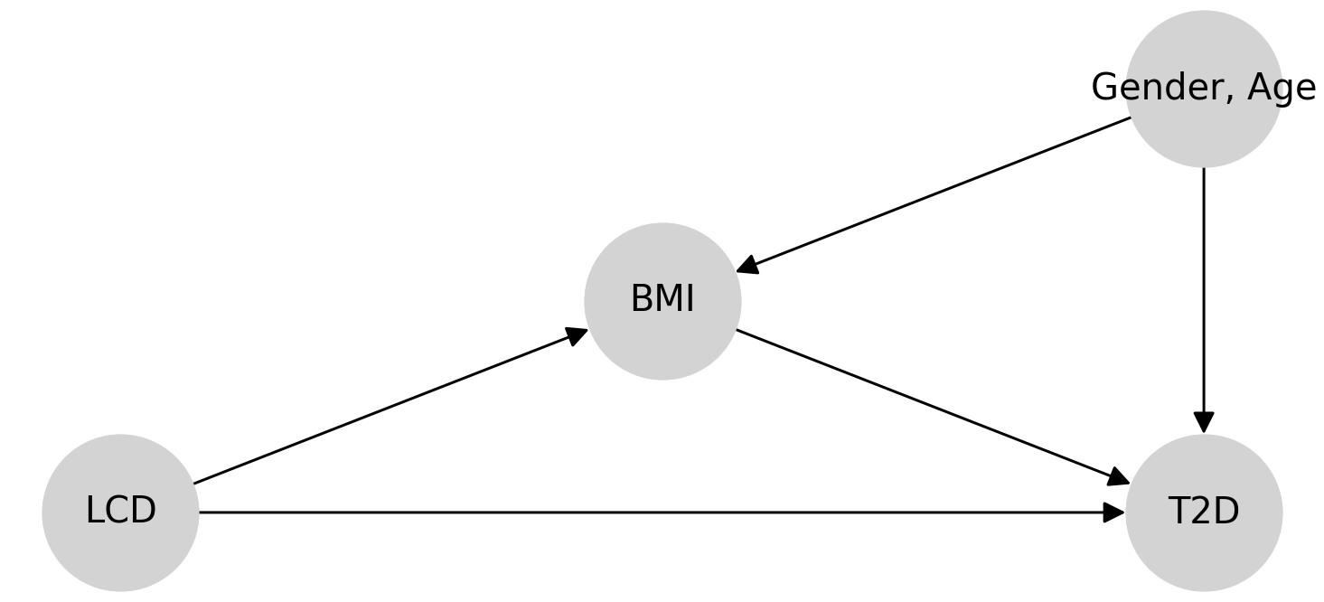
We will analyze the effect of LCD on the likelihood of developing T2D using Figure 1 after describing the structure of our dataset and reviewing causal inference basics.

2.2 Data

Our work is based on routine clinical data concerning 256 patients collected between 2013 and 2019 at the Norwood General Practice Surgery in the north of England ². As background, Norwood serves a stable population of approximately 9,800 patients, and an eight-fold increase in T2D cases was recorded over the last three decades.

Each patient visited the Norwood General Practice Surgery twice. The average time between visits was 23 months with a standard deviation of 17 months. Each patient is offered to start an LCD subsequent to the first visit. Measurements of standard indicators such as age, gender, weight, HbA1c, lipid profiles, and blood pressure were taken at both visits. Since CVD includes a range of clinical conditions such as stroke, coronary heart disease, heart failure, and atrial fibrillation ²¹, several different risk factors are recorded for CVD during individuals’ visits. We study four risk factors that indicate CVD risk. These are systolic blood pressure, serum cholesterol level, high-density lipoprotein, and a widely used measure of CVD risk called the Reynolds risk score, which is designed to predict the risk of a future heart attack, stroke, or other major heart disease. The Reynolds risk score is a linear combination of different risk factors such as age, blood pressure, cholesterol levels and smoking habits ²². A complete list of variables along with definitions and summary statistics is in Appendix C.

2.3 Model of potential outcomes

We use concepts and notations from the Neyman (or Neyman-Rubin) model of potential outcomes ^{23, 24}. The treatment assignment for individual $i$ is denoted by $T_{i}$, where $T_{i}=0$ and $T_{i}=1$ represent control and treatment. Let $Y_{i}$ be the observed outcome and $X_{i}$ be the observed confounders. For example, $X_{i}$ represents gender and age in the motivating example. The causal effect for individual $i$ is defined as the difference between the outcome if $i$ receives the treatment, $Y_{i}(1)$, and the outcome if $i$ receives the control, $Y_{i}(0)$. Since, in practice, an individual cannot be both treated and untreated, we work with two populations: a group of individuals exposed to the treatment and a group of individuals exposed to the control. It is important to distinguish between the observed outcome $Y_{i}$ and the counterfactual outcomes $Y_{i}(1)$ and $Y_{i}(0)$. The latter are hypothetical and may never be observed simultaneously; however, they allow a precise characterization of questions of interest. For example, the causal effect for individual $i$ can be written as the difference in potential outcomes:

$$\tau(X_{i})=\mathbb{E}[Y_{i}(1)|X_{i}]-\mathbb{E}[Y_{i}(0)|X_{i}].$$

Since the outcome surface $\tau(X)$ depends on confounders, we focus on the “average treatment effect" (ATE), $\mathbb{E}_{X}[\tau(X)]$, which is defined as the average causal effect for all individuals including both treatment and control.

1:Define a distance measure for determining whether or not an individual is a good match for another. For example, let the distance measure $D_{ij}=|e_{i}-e_{j}|$, which is based on propensity score $e_{i}(X_{i})=P(T_{i}=1|X_{i})$. We estimate $e_{i}$ by logistic regression for the case studies in Sections 5 and 4.

2:Given the distance measure, implement a matching method. For example, we apply matching with replacement and select a set of comparison units using the nearest-neighbor method in our case studies. Then we calculate ATE by

$$\frac{1}{n}\sum_{i}\left(Y_{i}-\frac{1}{|J_{i}|}\sum_{j\in J_{i}}Y_{j}\right),$$

where $n$ is the sample size, $J_{i}$ is the set of individuals that belong to a different group (i.e., treatment or control group) than the individual $i$ and are matched to $i$, and $|\cdot|$ denotes the number of elements in the set.

3:Assess the quality of the matched samples and iterate with steps 1 and 2 until samples are well matched. Output ATE.

Algorithm 1 Review of the propensity score matching algorithm

Matching methods attempt to eliminate bias in estimating the treatment effect from observational data by balancing observed confounders across treatment and control groups; see, e.g., Rubin and Thomas ²⁵ and Imbens ²⁶. These works identify two assumptions on data that are required in order to apply matching methods in an observational study.

• The strong ignorability condition (Rosenbaum and Rubin ²⁷) is referred to as the combination of exchangeability and positivity, which we discuss later that they are satisfied in our experiments.

  • Treatment assignment is independent of the potential outcomes given the confounders.

  • There is a non-zero probability of receiving treatment for all values of $X$: $0<\mathbb{P}(T=1|X)<1$.

  Weaker versions of the ignorability assumption exist; see, e.g., Imbens ²⁶.

• The stable unit treatment value assumption (SUTVA; Rubin ²⁸), which states that the outcomes of one individual are not affected by treatment assignment of any other individuals. There are two parts of the SUTVA assumption, which we rely on later in this paper.

  • No-interference: The outcome for individual $i$ cannot depend on which treatment is given to individual $i^{\prime}\neq i$. (Rubin ²⁸ attributes this to Cox ²⁹.)

  • No-multiple-versions-of-treatment: There can be only one version of any treatment, as multiple versions might give rise to different outcomes. (Rubin ²⁸ attributes this to Neyman ³⁰.)

“Version" refers to detailed information that is ignored as we coarsen a refined indicator to be used as a (typically binary) treatment. The assumptions mentioned above are complementary to the assumptions that determine causal models such as the one shown in Figure 1. To determine if treatment $T$ is ignorable relative to outcome $Y$, conditional on a set of matching variables, we require only that matching variables block all the back-door paths between $T$ and $Y$, and that no matching variable is a descendent of $T$ ³¹. For example, LCD in Figure 9 is ignorable since matching the confounders (i.e., gender and age) blocks all the back-door paths and the confounders are not descendants of LCD. The algorithm for propensity score matching is summarized in Algorithm 1. Detailed discussions of each step are deferred to Appendix A.

2.4 I-Rand algorithm

Two-point time-series datasets that are structurally similar to the nutrition dataset introduced in Section 2.2 arise frequently in medical and health studies. A dataset of this type consists of a baseline observation at time $t=0$ and a follow-up observation at $t=1$, where all individuals receive a treatment between the two time points. How do we apply matching methods to estimate the causal effect of a treatment that was taken between the two time points from a dataset of this type? To address this question, we look at what happens when we attempt to apply statistical methods to estimate the causal effect. Although there are many popular machine learning methods for causal estimation ^{32, 33}, we focus on two widely used approaches: pooling and difference-in-differences.

Pooling ^{14, 15} combines the baseline and the follow-up observations into a single dataset. This approach treats the measurements from individual $i$ at $t=0$ (before taking the treatment) and $t=1$ (after observing the outcome of the treatment) as distinct data points. This amounts to using observations at $t=0$ as a control group. Difference-in-differences ^{16, 17}, on the other hand, makes use of longitudinal data from both treatment and control groups to obtain an appropriate counterfactual to estimate causal effects. This approach compares the changes in outcomes over time between a population that takes a specific intervention or treatment (the treatment group) and a population that does not (the control group).

Consider the motivating example in Section 2.1, where every individual embarks on the LCD treatment at time 0. At time 1, we look at at how the outcome T2D is affected by the LCD between times 0 and 1, under numerous assumptions. Suppose we try to estimate the average treatment effect of the LCD by matching propensity scores on a dataset obtained by pooling observations at times 0 and 1. Since, for every $i$, the treatment $T_{i,t}$ determines the treatment $T_{i,1-t}$ the outcome for individual $i$ at time $t$ depends on the treatment of individual $i$ at time $1-t$. In other words, the pooled approach violates the no-interference assumption, and propensity score matching is not supported.^{14, 15}. As we illustrate with simulation in Section 3.1.1, the no-interference violation can lead to sub-par performance of causal estimates based on pooling. On the other hand, applying difference-in-differences to the motivating example would require us to make an assumption about what what would happen to individuals not treated between times $0$ and $1$. We explore this in Section 3.1.2.

The issues outlined above prompted us to develop I-Rand, a novel approach to estimating causal effects from two-point time-series data. As we show in simulation, I-Rand can reduce estimation error introduced by violations of the SUTVA assumption incurred by pooling data. There is some conceptional overlap between I-Rand and the synthetic control method ^{34, 35}, which provides a systematic way to choose comparison units (i.e., “synthetic control”) as a weighted average of all potential comparison units that best resembles the characteristics of the unit of interest (i.e., treatment unit). In I-Rand, both the control and treatments units are chosen from the data to form a “synthetic subsample” from which the causal effect is estimated using propensity score matching (i.e., the one control unit with the closest propensity score to the treatment unit of interest).

I-Rand samples one of the two visits for each patient, calculates the ATE on this selected subsample, and shuffles the treatment of the subsample to estimate the significance of the treatment. The estimation relies on the matching method described in Section 2.3 and applies a permutation test to the statistics estimated from the matching methods on the subsamples to infer the significance. Under the null hypothesis, the empirical ATEs are identically distributed. Formally, we construct a subsample in which each patient appears exactly once, either at $t=0$ or $t=1$ with the same probability, and then calculate the ATE from this sample. Then we construct additional $(M-1)$ subsamples, where each additional subsample should be drawn to have as few common observations with existing subsamples as possible. For example, one can apply the Latin hypercube sampling ³⁶ to draw the subsamples. We calculate the ATEs from the constructed $(M-1)$ subsamples and take the average ATE:

$$\frac{1}{M}\sum_{m=1}^{M}\text{ATE}^{(m)},$$ (1)

where $m$ indicates the $m$th generated subsamples. Then the i-Randomization estimator in Equation (1) gives the overall estimated ATE. To assess the significance of the treatment, we add another layer of randomization by permuting the treatments in the subsample. That is, given a subsample $m$ with corresponding estimand $\text{ATE}^{(m)}$, we shuffle the treatment vector of this subsample without changing the confounders or the outcome. We then estimate an average treatment effect $\text{ATE}^{(m,s)}$ for this shuffled treatment, where the superscript $(m,s)$ indicates that we have selected the subsample $m$ and the shuffle $s$. We repeat the experiment $S$ times (for a fixed subsample $m$), and obtain the distribution of average treatment effects., i.e., $(\text{ATE}^{(m,s)})_{s\in\{1,...,S\}}$. Then we calculate a p-value as the fraction of permuted average treatment effects that exceed the estimand $\text{ATE}^{(m)}$. The additional complexity of I-Rand is justified by the benefits that it brings relative to the pooled approach and difference-in-differences. I-Rand overcomes the SUTVA violation that is inherent in the pooled approach, and it creates a synthetic control group, which is absent in difference-in-differences. The I-Rand algorithm is summarized in Algorithm 2.

1:Input: $2n\times p$ data matrix where each row is attributes of an individual $i\in\{1,\ldots,n\}$ at time point $\in\{0,1\}$, and $p$ is the number of variables including the treatment, confounder, and outcome.

2:for $m=1,2,\ldots,M$ do

3:  Sample a binary vector of length $n$, where the index is the individual’s ID and the value is the time point (sampling without replacement). Select the corresponding subsample $m$;

4:  Calculate $\text{ATE}^{(m)}$ by the matching method;

5:  for $s=1,2,\ldots,S$ do

6:    Shuffle the vector of treatment;

7:    Calculate $\text{ATE}^{(m,s)}$ for the shuffle $s$ of the treatment from subsample $m$;

8:  end for

9:  Calculate $\text{p-val}^{(m)}=\frac{1}{S}\sum_{s=1}^{S}\mathbbm{1}_{\text{ATE}^{(m,s)}>(\text{resp. }<)\text{ATE}^{(m)}}$. That is, the p-value for the one-tailed test for the null hypothesis of no treatment effect.

10:end for

11:Output: The mean of ATEs $=\frac{1}{M}\sum_{m=1}^{M}\text{ATE}^{(m)}$; The mean of the p-values: $\frac{1}{M}\sum_{m=1}^{M}\text{p-val}^{(m)}$.

Algorithm 2 I-Rand algorithm

We note that the permutation test in I-Rand is valid only if the rearranged data are exchangeable under the null hypothesis ³⁷. In our two-sample test for the nutrition dataset, the exchangeability condition holds since the distributions of the two groups of data are the same under the null hypotheses that there is no treatment effect. The subsampling technique in I-Rand is similar to the one studied by Hahn ¹³ in the analysis of spatial point patterns. The difference, however, is that the normalization of test statistics (i.e., ATE) is unnecessary in I-Rand since the matching method has balanced the designs.

3 Comparison of I-Rand with Alternative Methods

We use simulation to compare errors in an I-Rand-based estimation of a treatment effect with errors from the pooled approach and difference-in-differences. We look at causal effect estimation under two types of treatment assignments inspired by our data and the questions considered in this article. First, we study the “LCD-like treatment", as in the motivating example in Section 2.1, where $T=0$ at $t=0$ and $T=1$ at $t=1$ for all individuals. The LCD-like treatment respects the two-point time series structure since the assignment of $T$ depends on time.

Next, we consider a study from Section 5.1: does obesity cause T2D? Here, treatment is a binary indicator based on the body-mass index (BMI), where obesity is indicated by ${\rm BMI}>30$. To avoid excess notation, we use the acronym “BMI" to indicate both the body mass index and the binary treatment derived from it. In this study, there is a control group consisting of individuals with BMI < 30. This treatment does not align with time, and we call treatments of this type “BMI-like." Here, it is natural to pool the data at the two time points, with a control group of non-obese individuals and a treatment group of obese individuals. To apply difference-in-differences, we split the data into two subsets. The first subset consists of individuals who are non-obese at time 0. The control group in the subset is individuals who are non-obese at time 1, while the treatment group consists of individuals who are obese at time 1. For this subset, the treatment, obesity, has a significant effect on T2D if change in T2D is significantly different in the treatment group than in the control group. The second subset consists of individuals who are obese at time 1. The control group in the subset is individuals who are obese at time 1, while the treatment group consists of individuals who are non-obese at time 1. Again, the treatment, obesity, causes T2D if the change in T2D is significantly different from zero in the treatment group than in the control group. As usual, the numerous assumptions on which our results rely include causal completeness. We note that, while it may be unintuitive, it is certainly possible that the effect of increased obesity on T2D could turn out to be negative. An overview of the comparison of I-Rand with two benchmark methods is given in Table 1.

Table 1: Overview of comparison of I-Rand with alternative methods given two-point time-series with novel structures

	Respect time structure	Ignore time structure
	(LCD-like treatment)	(BMI-like treatment)
Pooled approach vs. I-Rand	Section 3.1.1	Section 3.2.1
Difference-in-differences vs. I-Rand	Section 3.1.2	Section 3.2.2

All our simulations consider a panel dataset with two time points where outcomes are specified by the structural equation:

$$Y_{i,t} =\alpha+f(T_{i,t})+g(X_{i,t})+\varepsilon^{Y}_{i,t},$$ (2)

where the confounder vector $X_{i,t}$, such as age or gender, takes continuous or categorical values. The parameter $\alpha\in\mathbb{R}$, and $f(\cdot)$ and $g(\cdot)$ are unknown functions that satisfy the condition $\mathbb{E}_{T}[f(T)]=\mathbb{E}_{X}[g(X)]=0$ to ensure identifiability of model (2). Assuming the confounder satisfies the back-door criterion ³¹, we can interpret $f(\cdot)$ as the causal mechanism of $T$ affecting $Y$ ³⁹. The noise term $\varepsilon^{Y}_{i,t}$ is assumed to be i.i.d. for any $i$ and $t$, and has zero mean and bounded variance. The treatment $T_{i,t}$ is specified differently in different examples that we consider below.

3.1 Time-aligned (LCD-like) treatment

To complete the specification of the data generating process (2), we set the treatment variable as follows:

$$T_{i,t}=\mathbbm{1}_{t=1},\quad\forall i\in\{1,\ldots,n\}\text{ and }t\in\{0,1\},$$ (3)

where the treatment $T_{i,t}$ for individual $i$ at time $t$ is binary and depends only on time. For example, $T_{i,t}$ in the nutrition data of Section 2.2 indicates whether individual $i$ follows an LCD at time $t$. The outcome $Y_{i,t}$ is analogous to the HbA1c measure in the nutrition data of Section 2.2. We note that the strong ignorability condition in Section 2.3 is satisfied under the LCD-like treatment (3). Specifically, the first condition on exchangeability holds since the $T=1$ is independent of the potential outcomes given the confounders under (3). The second condition on positivity holds because for any given confounders $X$ that excludes the time $t$, the probability of receiving treatment satisfies $0<\mathbb{P}(T=1|X)<1$. However, the data-generating process under (3) violates SUTVA in Section 2.3.

3.1.1 Comparison to the pooled approach

The pooled approach breaches the “no-interference” assumption as $T_{i,t}$ determines $T_{i,t^{\prime}}$, where $t\neq t^{\prime}\in\{0,1\}$. Thus, each pair of distinct observations has the same probability of being matched, which violates the “no-interference” assumption of the SUTVA in Section 2.3. We refer readers to Appendix A for an overview of the propensity score matching.

We consider a numerical example that illustrates the consequence of breaching the “no-interference” assumption on the pooled data. We consider a correlated structure of confounders that simulates the age and gender in the nutrition data of Section 2.2, where

$$X_{i,0} =\varepsilon_{i}^{X},\quad\varepsilon_{i}^{X}\sim N(0,1),$$ (4)

$$X_{i,1} =\rho X_{i,0}+\sqrt{1-\rho^{2}}\xi_{i}^{X}+a^{X}t,\quad\xi_{i}^{X}\sim N(0,1),$$

where $\rho$ is the correlation between the confounder at $t=0$ and at $t=1$, and $a^{X}$ is a drift term. We set $\rho=1$ and $a^{X}=0$ in this simulation. It is the case when the confounder used is unchanged with the passage of time, i.e., fixed attributes like gender or ethnicity. The outcome $Y_{i,t}$ is generated by letting $f(\cdot)$ and $g(\cdot)$ in (2) be linear functions:

$$f(T)=T\delta,\quad g(X)=X\beta.$$ (5)

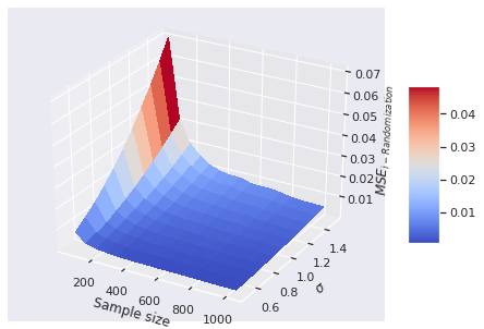
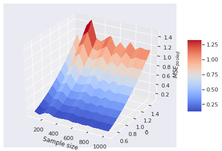
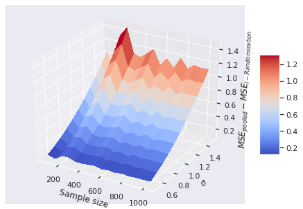
Here $\alpha$ in (2) is set to $0$, and $\beta=-1$ and $\delta=1$ in (5). The noise variable $\varepsilon^{Y}_{i,t}$ in (2) is independently drawn from $N(0,\sigma^{2})$. Under the pooled approach, we estimate the treatment effect based on the propensity score matching in Algorithm 1. Under I-Rand, we estimate the treatment effect by averaging over the estimates using $100$ subsamples using Algorithm 2. Figure 2 reports the mean squared errors (MSEs) for $\delta$ with varied sample sizes and noise levels. In our example, I-Rand outperforms the pooled approach, whose ATE estimate has inflated error due to the breach of “no-interference” assumption.

Figure 2: The MSE for the estimate of treatment effect when varying the sample size and noise level $\sigma$. Left plot: the MSE surface for the I-Rand; Middle plot: the MSE surface for the pooled approach; Right plot: $\text{MSE(pooled)}-\text{MSE(I-Rand)}$.

3.1.2 Comparison to difference-in-differences

The standard set up of difference-in-differences ^{16, 17} is one where outcomes are observed for two groups for two time periods. One of the groups is exposed to a treatment in the second period but not in the first period. The second group is not exposed to the treatment during either period. In the case where the same units within a group are observed in each time period, the average gain in the control group is substracted from the average gain in the treatment group, which gives an estimate to the average treatment effect:

ATE $$\equiv\mathbb{E}_{X}[\mathbb{E}[Y_{i}(t=1)-Y_{i}(t=0)|T_{i}(t=1)=1,T_{i}(t=0)=0,X]]$$ (6)

$$\quad-\mathbb{E}_{X}[\mathbb{E}[Y_{i}(t=1)-Y_{i}(t=0)|T_{i}(t=1)=0,T_{i}(t=0)=0,X]].$$

Difference-in-differences removes biases in second period comparisons between the treatment and control group that could be the result from permanent differences between those groups, as well as biases from comparisons over time in the treatment group that could be the result of trends. We note that this standard difference-in-differences approach does not require the knowledge of the functions $f(\cdot)$ or $g(\cdot)$ in (2). However, in our application with the LCD-like treatment design (3), the treatment effect (6) cannot be estimated from data using the aforementioned standard approach of difference-in-differences. The main reason is that LCD-like treatment design lacks the control group $\{i|T_{i}(t=1)=0,T_{i}(t=0)=0\}$. We summarize this result in the following theorem.

Theorem 3.1.

Under the two-point treatment design (3) and the structural equation (2), the treatment effect (6) is not identifiable by difference-in-differences if there is no prior knowledge on the parametric family of $f(\cdot)$ and $g(\cdot)$ in (2).

The proof of Theorem 3.1 is in Appendix B. The theorem suggests that the difference-in-differences is not applicable under the two-point treatment design (3). By contrast, the I-Rand in Algorithm 2 constructs a synthetic control group by randomly selecting one of the two points for each individual, and it can identify and estimate the treatment effect (6) from data.

A remedy for applying difference-in-differences to the treatment design (3) is assuming a parametric functional form of $f(\cdot)$ and $g(\cdot)$ in the structural equation (2). For example, one can assume $f(\cdot)$ and $g(\cdot)$ to be linear functions (5). The treatment effect $\delta$ can be estimated by regressing over the observational treatment group data $\{i|T_{i}(t=1)=1,T_{i}(t=0)=0\}$ under the design (3). Nonetheless, we demonstrate that even in a parametric structural equation, I-Rand can outperform difference-in-differences. We simulate data using formulas (2) to (5). The outcome $Y_{ij}$ is calculated using (5) with $\alpha=0$, $\beta=-1$, and $\delta=1$, whereas the errors $\varepsilon^{Y}_{i,t}$ are i.i.d drawn from $N(0,\sigma^{2})$. In (4), we set $\rho=0.99$ and $a^{X}=1/12$, leading to similar values of the covariates for each individual at the two time points as the nutrition data in Section 2.2, and a passage of time equal to one month. We take the difference in the variables in both sides of the equation (2) and obtains

$$DY_{i}=DT_{i}\delta+DX_{i}\beta+D\varepsilon_{i}^{Y},$$ (7)

where the operator $D$ denotes the difference in the variable between $t=1$ and $t=0$, i.e., $DZ_{i}=Z_{i,t=1}-Z_{i,t=0}$ for any variable $Z$. In this example, the propensity score matching is not applicable to difference-in-differences . We apply least squared regression to model (7) and use the observational treatment group data $\{i|T_{i}(t=1)=1,T_{i}(t=0)=0\}$ to estimate the parameter $\delta$. For I-Rand, we apply Algorithm 2 and obtain the treatment effect by averaging over $100$ subsamples. Difference-in-difference estimates are obtained by least squared regression on (7), as explained above.

Figure 3 reports the mean-squared errors to the true value $\delta=1$ (left panel), and the difference in MSEs between i-Rand and DiD, when varying sample sizes and noise levels. From the plots, we see that i-Rand has small MSEs and that MSEs for DiD are larger than MSEs for i-Rand. While linear regression is subject to large estimation error because of the high correlation between change in the treatment vector ($DT$) and change in age ($DX$), the absence of a control group ($DT=0$) makes the passage of time (increase in age) as likely to be responsible for the change in outcome as the treatment itself. While the poor performance of difference-in-differences can be traced to the lack of a control group, an estimation using regression does not always fail and could still give good results when the treatment and confounders are uncorrelated. Our example illustrates how regressions can fail to estimate a causal effect.

Figure 3: The MSE for the estimate of treatment effect when varying the sample size and noise level $\sigma$. Left plot: the MSE surface for the I-Rand; Middle plot: the MSE surface for the DiD approach; Right plot: $\text{MSE(difference-in-differences)}-\text{MSE(I-Rand)}$.

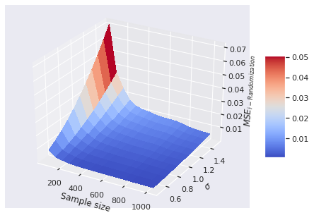
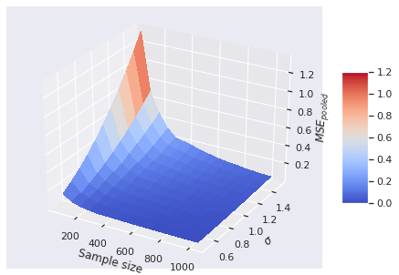
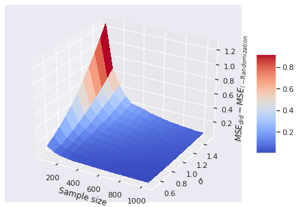
We summarize in Table 2 the advantages of I-Rand compared to two benchmark approaches for the LCD-like treatment.

Table 2: Comparison of three approaches in the case of the LCD-like treatment in Section 3.1

	Pooled approach	Difference-in-differences	I-Rand
SUTVA assumption	Fail	Hold	Hold
Control group	Yes	No	Yes

3.2 Time misaligned (BMI-like) treatment

To complete the specification of the data generating process (2), we set the treatment variable as follows:

$$T_{i,t}=h(X_{i,t}),\quad\forall i\in\{1,\ldots,n\}\text{ and }t\in\{0,1\}.$$ (8)

Here the treatment $T_{i,t}$ for individual $i$ at time $t$ is a binary function of the confounders $X_{i,t}$.

Our treatment is time misaligned because it ignores our two-point time-series structure, i.e., two observations for each patient with treatment administrated at $t=0$ and observed at $t=1$. It mimics the experiment in Section 2.2, where the treatment is a discrete version of BMI: $T_{i,t}$ is weight category (e.g., normal or overweight) of individual $i$ at time $t$. In this experiment $T_{i,t}$ depends on the confounders such as LCD, age and gender.

3.2.1 Comparison to the pooled approach

Unlike the LCD-like assignment in Section 3.1.1, the pooled approach ^{14, 15} meets the SUTVA assumption of “no-interference” under design (8). Moreover, the pooled approach provides an estimate to $\text{ATE}^{*}$ in (14) by treating the observations from an individual at $t=0,1$ as two distinct data points. We demonstrate through numerical examples that the pooled approach is a comparable alternative to I-Rand in the BMI-like treatment assignment (8).

Figure 4: The MSE for the estimate of treatment effect when varying the sample size and noise level $\sigma$. Left plot: the MSE surface for the I-Rand; Middle plot: the MSE surface for the pooled approach; Right plot: $\text{MSE(pooled)}-\text{MSE(I-Rand)}$.

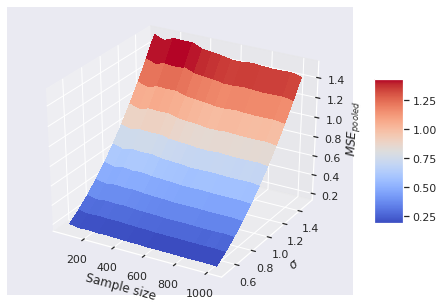
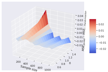
We specify the confounder $X=(X^{(1)},X^{(2)})$, where $X^{(1)}$ denotes an individual’s age and $X^{(2)}$ indicates whether or not an individual has followed an LCD. Age, $X^{(1)}$, follows the confounder generating process in (4) with correlation $\rho=0.99$ and passage of time $a^{X}=1/12={\rm one~{}month}$. (The parameter $a^{X}$ in (4) is analogous to the time trend in the nutrition data in section 2.2.) The LCD-indicating confounder $X^{(2)}$ is set to $X^{(2)}_{i,t}=\mathbbm{1}_{t=1}$. Treatment is assigned according to $T_{i,t}=\mathbbm{1}_{\varepsilon^{T}_{i,t}>0}$ where $\varepsilon^{T}_{i,t}=X^{(2)}_{i,t}+\xi^{T}_{i,t}$ where $\xi_{i,t}^{T}\sim N(0,1)$. We consider the linear model (5) for outcome $Y_{i,t}$, where $\varepsilon_{i,t}^{Y}\sim N(0,\sigma^{2})$, and $\alpha=0$, $\beta=(-1,1)$, and $\delta=1$. The results are displayed in Figure 4, where the MSE surface for I-Rand is shown with varying sample size and noise level $\sigma$. Also displayed is the difference between the MSE of I-Rand and the pooled approach. I-Rand performs similarly to the pooled approach in our simulation, lending support to the assertion that the approaches are comparable for the BMI-like treatment (8).

3.2.2 Comparison to difference-in-differences

In the time misaligned BMI-like treatment, difference-in-differences ^{16, 17} encounters the problem of having four different types of individuals; always-treated ($\{i|T_{i}(t=1)=1,T_{i}(t=0)=1\}$), never-treated ($\{i|T_{i}(t=1)=0,T_{i}(t=0)=0\}$), treated-to-untreated $\{i|T_{i}(t=1)=0,T_{i}(t=0)=1\}$, and untreated-to-treated $\{i|T_{i}(t=1)=1,T_{i}(t=0)=0\}$. To obtain an estimate of the treatment effect in this case, it is necessary to compare the outcomes of the group of never-treated to untreated-to-treated or the outcomes of the group of always-treated to treated-to-untreated. The idea is that the treatment state should be the same in both groups at $t=0$ and different at $t=1$. We illustrate our ideas on the former; the latter follows the same line of reasoning. Difference-in-differences gives an estimate of the causal effect in (6), which is the same as the target effect $\text{ATE}^{*}$ in (14) only if

$$\mathbb{E}_{X}[\mathbb{E}[Y_{i}(t=0)|T_{i}(t=1)=1,T_{i}(t=0)=0,X]]=\mathbb{E}_{X}[\mathbb{E}[Y_{i}(t=0)|T_{i}(t=1)=0,T_{i}(t=0)=0,X]],$$ (9)

$$\text{ or }\quad\mathbb{E}_{X}[\mathbb{E}[Y_{i}(t=1)|T_{i}(t=1)=0,T_{i}(t=0)=0,X]]=\mathbb{E}_{X}[\mathbb{E}[Y_{i}(t=0)|T_{i}(t=1)=0,T_{i}(t=0)=0,X]].$$ (10)

However, both (9) and (10) are strict and likely to fail in practice. Take the nutrition data in Section 2.2 as an example. Condition (9) requires that the expected outcome at the baseline is the same between two different groups: $\{i|T_{i}(t=1)=1,T_{i}(t=0)=0\}$ and $\{i|T_{i}(t=1)=0,T_{i}(t=0)=0\}$. However, the unobserved confounders such as lifestyle and genetic information in the two groups $\{i|T_{i}(t=1)=1,T_{i}(t=0)=0\}$ and $\{i|T_{i}(t=1)=0,T_{i}(t=0)=0\}$ are different (otherwise the treatment at $t=1$ should be the same in two groups), so that condition (9) is likely to fail. Moreover, condition (10) requires the expected outcomes be the same at the two time points, $t=0,1$, for the group $\{i|T_{i}(t=1)=0,T_{i}(t=0)=0\}$. However, since an individual does not take an LCD at $t=0$ and does take an LCD at $t=1$, the confounder LCD assignment differs between $t=0$ and $t=1$. Hence the condition (10) would fail for the nutrition data in Section 2.2.

Consequently,difference-in-differences (6) cannot be applied to the BMI-like treatment assignment (8). An alternative approach to implementing difference-in-differences is directly applying regression to a difference of parametric structural equation models. Specifically, we apply regression to (7). We consider the simulation setup in Section 3.2.1 and find that the estimate of the causal effect with difference-in-differences is unstable. The results are in Figure 5, where the MSE surface for I-Rand is shown with varying sample size and noise level $\sigma$. Also shown is the difference between the MSE of I-Rand and the MSE of the benchmark, difference-in-differences. We notice in the small sample size regime, I-Rand outperforms difference-in-differences.

Figure 5: The MSE for the estimate of treatment effect when varying the sample size and noise level $\sigma$. Left plot: the MSE surface for the I-Rand; Middle plot: the MSE surface for the DiD approach; Right plot: $\text{MSE(difference-in-differences)}-\text{MSE(I-Rand)}$.

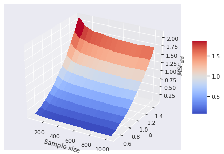
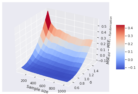
To conclude this section, we stress that the first argument in favor of the application of I-Rand is its verification of the SUTVA assumption in both the time-aligned and time-misaligned treatments we considered. The estimation of the causal effect is data dependent, but we find that I-Rand performs at least as well as the benchmark methods in the examples considered. Naturally, I-Rand is also subject to some limitations. One of them is the dependence of the estimates across subsamples inflate the variance estimate. This can be mitigated by minimizing overlaps in subsamples.

4 Case Study I: Can Diet Lower the Risk for T2D and CVD?

4.1 Treatment effect of LCD on T2D

We can now analyze the motivating example introduced in Section 2.1 and give an answer to the counterfactual question: If an individual changes from a regular diet to an LCD diet, would he / she be less likely to develop T2D? The LCD restricts consumption of carbohydrates relative to the average diet ⁷. Several systematic reviews and meta-analyses of randomized control trials suggest beneficial effects of LCD in T2D and CVD, including improving glycaemic control, triglyceride and HDL cholesterol profiles ^{8, 9, 10}. However, the impact of LCD in a “real world" primary care setting with observational data and its cause-and-effect inferences has not been fully evaluated ². The challenges of analyzing routine clinical data include the irregular treatment assignments. For example, our analysis relies on the two-point time-series data without control group described in Section 2.2, where all patients participated in the program are suggested to change from their regular diets to LCD after their initial visit to the clinic. The irregular design of treatments limit the applications of benchmark methods such as pooled approach and difference-in-differences as discussed Section 3. In this section, we apply the proposed I-Rand algorithm to analyze the real data described in Section 2.2.

The analysis using observation data utilizes the model of potential outcomes in Section 2.3. According to the causal graph in Figure 1, LCD takes the role of a treatment that affects the mediator BMI and outcome T2D. Gender and age affect BMI and T2D, but not the treatment LCD. To quantify the expected change in T2D if BMI were changed, we need to calculate the total causal effect of LCD on T2D, which can be characterized by the ATE:

$$\mathbb{E}[\tau_{1}(\text{Gender}_{i},\text{Age}_{i})],$$

where the potential outcome $\tau_{1}$ (with “$1$" indexing that this is the first of a series of nutrition questions) is defined as

$$\tau_{1}(\text{Gender}_{i},\text{Age}_{i})=\mathbb{E}[\text{T2D}_{i}(\text{LCD}=1)\ |\ \text{Gender}_{i},\text{Age}_{i}]-\mathbb{E}[\text{T2D}_{i}(\text{LCD}=0)\ |\ \text{Gender}_{i},\text{Age}_{i}].$$

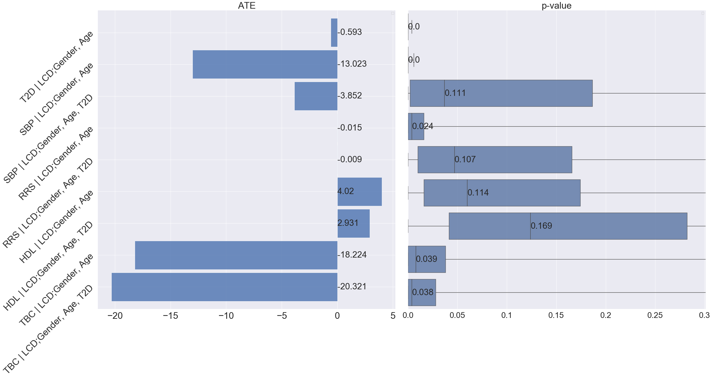
We control for the confounders (i.e., gender and age) ³¹ to estimate the ATE and assess the significance by the proposed I-Rand algorithm. We implement I-Rand by drawing $500$ subsamples and calculate the ATE of each subsample. Then, we perform the permutation test for each subsample to evaluate the significance level of the ATE. The result provided in Table 3 indicates that LCD would significantly decrease in the risk of T2D, which is also supported by the box plot of p-values in the first row of Figure 7, and the distributions of ATEs and p-values in Appendix D.1, where the results show the consistency of the significant causal effects across random subsamples. We make four remarks on the application of I-Rand and the experimental results of this example.

First, there is no control group with individuals on a regular diet at two visits. This is because all individuals were at risk of developing T2D or with T2D and thus suggested to begin the LCD after their first visit. The application of the I-Rand algorithm in this example not only avoids a violation of the SUTVA assumption, but more importantly, to artificially construct synthetic control group. The way that I-Rand constructs synthetic control group is different from the existing synthetic control method ³⁵. In particular, existing synthetic control method requires the available control individuals and constructs a synthetic control as a weighted average of these available control individuals. However, I-Rand does not require that there exists available control individuals. Instead, I-Rand constructs a synthetic control by subsampling one of the two time points of each individual.

Table 3: Causal analysis for the effect of LCD on T2D and Reynolds risk score for CVD

	LCD on T2D ($\mathbb{E}[\tau_{1}]$)		LCD on Reynolds risk score for CVD
		Total effect ($\mathbb{E}[\tau_{2}]$)	Direct effect ($\mathbb{E}[\tau_{3}]$)	Indirect effect ($\mathbb{E}[\tau_{4}]$)
ATE	-0.593	-0.015	-0.009	-0.005
p-value	0.001	0.024	0.107	0.003

Second, we note that under the null hypothesis of no causal effect, the p-values follow a uniform distribution on $(0,1)$ given sufficiently many subsamples. However, the box plot of p-values in the first row of Figure 7, corresponding to the causal graph in Figure 1, shows p-values are concentrated at the origin, which indicates a strong evidence for the alternative hypothesis. We note that the hypothesis testing is performed for each subsample independently, but the p-values are not independent across subsamples. This is because the subsamples are correlated although the correlation is weak given each subsample is randomly chosen from the pool of $2^{256}$ subsamples. If the concentration of the p-values is around $0$, we can say with confidence that a small p-value is not a coincidence of the subsample, if most p-values are large, we conclude that the significance of the treatment effect is questionable.

Third, for better appreciating the results in Table 3 we compare them with T2D risks from routine care without LCD suggestion. Some idea of the results that one might expect from routine care can be drawn from the data of control group in the DiRECT study ¹¹, which recently investigated a very low-calorie diet of less than $800$ calories and subsequent drug-free improvement in T2D, including T2D remission without anti-diabetic medication. At 12 months, DiRECT study gives $46\%$ of T2D remission, which is close the $45\%$ rate given in Table 3 from our dataset with LCD over an average of 23 months duration. As a comparison, DiRECT quotes a remission rate at 24 months of just $2\%$ for routine T2D care without dietary suggestion. This result emphasizes how rare remission is in usual care and the potential value of LCD to lower the T2D risk.

Finally, we note that our approach relies on individuals’ assertions of compliance to the LCD. For several years an LCD has generally been accepted as one containing less than 130 grams of carbohydrate per day ⁴⁰. However, it may not be realistic for individuals to count grams of carbohydrate in a regular basis. Our dataset collected from Norwood general practice surgery instead only give clear and simplified explanations of how sugar and carbohydrate affect glucose levels and how to recognize foods with high glycaemic loads ². The promising result in Table 3 shows that this simple and practical approach to lowering dietary carbohydrate leads to significant improvement in T2D without the need for precise daily carbohydrate or calorie counting.

4.2 Mediation analysis for the effect of LCD on CVD

Motivated by the fact that T2D was crucial in explaining CVD risk (Benjamin et al. ⁵), we seek to understand the role of T2D as a mediator of the effect of dietary on CVD risk. This is relevant from the perspective of clinical practice for an individual who is afflicted with both T2D and CVD, since he / she may be able to control factors besides T2D that contribute to CVD risk.

4.2.1 Causal graph of T2D as a mediator

We assume the causal graph in Figure 6. Note that the outcome CVD has many risk factors, including systolic blood pressure, serum cholesterol level, high-density lipoprotein (which is inversely correlated with CVD risk); see, e.g., Ridker et al. ²². We study these three well-known risk factors as well as the Reynolds risk score. We motivate Figure 6 with the following data-generating process: (1) Similar to Figure 1, choose the treatment LCD at random; Given a selected LCD, sample an individual with a corresponding BMI level; Conditional on the choice of LCD and BMI level, sample the T2D status as the medical outcome; (2) In addition to Figure 1: Conditional on the choice of LCD and T2D status, sample the medical outcome within a given CVD risk factor. The details are as follows. First, the arrows LCD $\to$ T2D and LCD $\to$ BMI encode that the distributions of T2D and BMI depend on LCD status. This dependence was quantified in Section 4.1. Second, the arrow T2D $\to$ CVD reflects the established knowledge in nutrition science that T2D influences CVD risk (Benjamin et al. ⁵, Martín-Timón et al. ⁴¹). Likewise, the arrow BMI $\to$ CVD translates the fact that obesity is a cardiovascular risk factor (Sowers ⁴²). Finally, since our model assumes causal sufficiency, the arrow LCD $\to$ CVD represents dietary-specific influences on CVD risk. In reality, there may be other mediators, such as socioeconomic status, culture occupation, and stress level. In addition to the causal graph in Figure 11, we assume there are no hidden confounders.

Figure 6: Assumed coarse-grained causal graph for the relationship between LCD, BMI, T2D, and the outcome CVD risk. Within this view, T2D acts as a mediator of the effect of LCD on CVD risk.

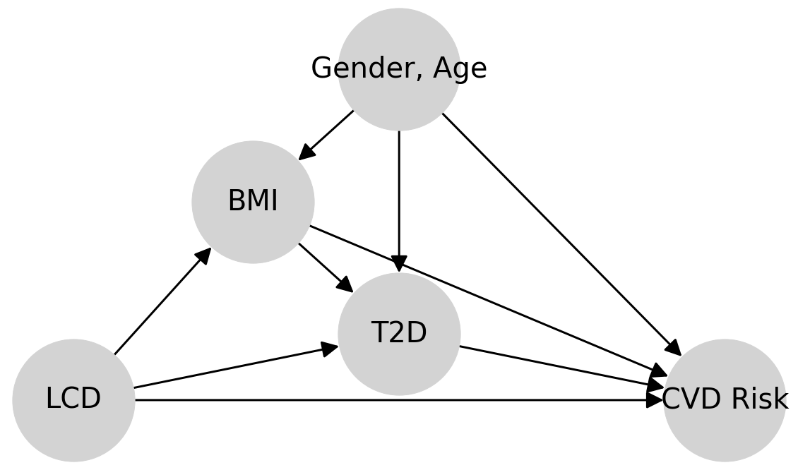
Given these assumptions, we see that LCD causally influences CVD risk along two different paths: a path LCD $\to$ CVD, giving rise to a direct effect, and two paths LCD $\to$ BMI $\to$ T2D $\to$ CVD and LCD $\to$ T2D $\to$ CVD, which are mediated by T2D and give rise to an indirect effect. Note that the direct effect of LCD on CVD risk is likely mediated by additional variables that are subsumed in LCD $\to$ CVD. We discuss this point further in Section 6. In mediation analysis, the goal is to quantify direct and indirect effects. We start with the total effect and then formulate the direct and indirect effects by allowing the treatment to propagate along one path while controlling the other path.

4.2.2 Total effect of LCD on CVD

Given the causal assumptions in the previous section, the first measure of interest is the total causal effect of LCD on CVD, i.e., the answer to the following question:

“What would be the effect on CVD if an individual changes from regular diet to LCD?"

We formulate the answer using the ATE:

$$\mathbb{E}[\tau_{2}(\text{Gender}_{i},\text{Age}_{i})],$$

where the potential outcome $\tau_{2}$ is defined as

$$\tau_{2}(\text{Gender}_{i},\text{Age}_{i})=\mathbb{E}[\text{CVD}_{i}(\text{LCD}=1)|\text{Gender}_{i},\text{Age}_{i}]-\mathbb{E}[\text{CVD}_{i}(\text{LCD}=0)|\text{Gender}_{i},\text{Age}_{i}].$$

Using the I-Rand algorithm, we report the results for the effect of LCD on the Reynolds risk score as measure of CVD risk. The total effect and the p-value are given in Table 3. Figure 7 summarizes the effects of LCD on all four measures of CVD risk. The LCD significantly lowered the Reynolds risk score (RRS), systolic blood pressure (SBP) and serum total cholesterol (TBC) but it did not have a statistically significant effect on good cholesterol (HDL). The promising result on the improvement of Reynolds risk score, systolic blood pressure and serum total cholesterol suggests that it may be a reasonable approach, particularly if an individual hopes to avoid medication, to offer LCD with appropriate clinical monitoring.

Figure 7: Mean ATE bar plot (left) and p-values box plot (right) for LCD as the treatment. Each row corresponds to a causal diagram:“Outcome $|$ Treatment; Confounders”. For example, “SBP $|$ LCD; Gender, Age” represents the causal diagram with the systolic blood pressure as the outcome, and gender and age as the confounders, and the LCD as the treatment.

4.2.3 Direct effect of LCD on CVD

We now study the natural direct effect (see, Pearl ⁴³) of LCD on CVD risk in the context of the following hypothetical question:

“For an individual of non-LCD taker, how would LCD affect the risk of CVD?"

We are asking what would happen if the treatment, LCD, were to change, but that change did not affect the distribution of the mediator, T2D. In that case, the change in treatment would be propagated only along the direct path LCD $\to$ CVD in Figure 6. We argue that the analysis in this situation should control for gender, age, and T2D, and a look at Figure 6 give an explanation ³¹. To disable all but the direct path, we need to stratify by T2D. This closes the indirect path LCD $\to$ T2D $\to$ CVD. But in so doing, it opens two paths LCD $\to$ T2D $\leftarrow$ (Gender, Age) $\to$ CVD, and LCD $\to$ BMI $\to$ T2D $\leftarrow$ (Gender, Age) $\to$ CVD. If we control for (Gender, Age) as well, we close these two paths, and therefore any correlation remaining must be due to the direct path LCD $\to$ CVD. We refer readers to Pearl ³¹ for an introduction to mediation analysis based on causal diagram.

To quantify the expected change in CVD if LCD status were changed, we need to control for calculate

$$\mathbb{E}[\tau_{3}(\text{Gender}_{i},\text{Age}_{i},\text{T2D})],$$

where the potential outcome $\tau_{3}$ is defined as

$$\tau_{3}(\text{Gender}_{i},\text{Age}_{i},\text{T2D}_{i}) =\mathbb{E}[\text{CVD}_{i}(\text{LCD}=1)|\text{Gender}_{i},\text{Age}_{i},\text{T2D}(\text{LCD}=0)]$$

$$\quad\quad-\mathbb{E}[\text{CVD}_{i}(\text{LCD}=0)|\text{Gender}_{i},\text{Age}_{i}].$$

The symbol T2D(LCD $=0$) is the counterfactual distributions of BMI and T2D given that the status of LCD is $0$. The expectations above are taken over the corresponding interventional (i.e., LCD $=0,1$) and counterfactual (i.e., T2D(LCD $=0$)) distributions. We implement I-Rand, which gives the direct effect for the Reynolds risk score in Table 3. Figure 7 summarizes the direct effects of LCD on all four measures of CVD risk. The LCD has a significant direct effect on lowering the Reynolds risk score (RRS) and serum total cholesterol (TBC) with the average p-value less than $10\%$. We complement the results shown in Figure 7 with the distributions of ATEs and p-values of the subsamples in Appendix D.2. The direct effect in this example represents a stable causal effect that, different from the total effect, is robust to T2D and any cause of CVD risk that is mediated via T2D. This robustness makes the natural direct effect a more actionable concept, and in principle, it can be transported to populations with different physical conditions such as T2D status.

4.2.4 Indirect effect of LCD on CVD

To isolate the indirect effect from the direct effect, we need to consider a hypothetical change in the mediator while keeping the treatment constant. In our CVD example, we may ask:

“How would the CVD risk of an individual without taking LCD be if his / her T2D status had instead following the T2D distribution of individuals taking LCD?"

The answer to this question is the average natural indirect effect (Pearl ⁴³). It can be written as

$$\mathbb{E}[\tau_{4}(\text{Gender}_{i},\text{Age}_{i},\text{T2D})],$$

where the potential outcome $\tau_{4}$ is defined as

$$\tau_{4}(\text{Gender}_{i},\text{Age}_{i}) =\mathbb{E}[\text{CVD}_{i}(\text{LCD}=0)|\text{Gender}_{i},\text{Age}_{i},\text{T2D}(\text{LCD}=1)]$$

$$\quad\quad-\mathbb{E}[\text{CVD}_{i}(\text{LCD}=0)|\text{Gender}_{i},\text{Age}_{i}].$$

The symbol $\text{T2D}(\text{LCD}=1)$ refers to the counterfactual distribution of T2D had LCD been 1, and the expectations are taken over the corresponding interventional (i.e., $\text{LCD}=0,1$) and counterfactual (i.e., $\text{T2D}(\text{LCD}=1)$) distributions. Under our assumptions, any changes that occur in an individual’s CVD risk are attributed to treatment-induced T2D and not to the treatment (i.e., LCD) itself.

Figure 8: Indirect Effect: Mean ATE bar plot (left) and p-values box plot (right) for the indirect effect of LCD on CVD risk factors with age, gender as confounders and diabetes as a mediator. Each row corresponds to a causal diagram:“Outcome $|$ Treatment; Confounders [Mediator]”. For example, “SBP $|$ LCD; Gender, Age [T2D]” represents the causal diagram with the systolic blood pressure as the outcome, gender, age, as the confounders, T2D as the mediator, and the LCD as the treatment.

For a linear model in which there is no interaction between treatment and mediator, the total causal effect can be decomposed into a sum of direct and indirect contributions (see, e.g., Pearl ⁴³):

$$\text{total effect}=\text{direct effect}+\text{indirect effect}.$$ (11)

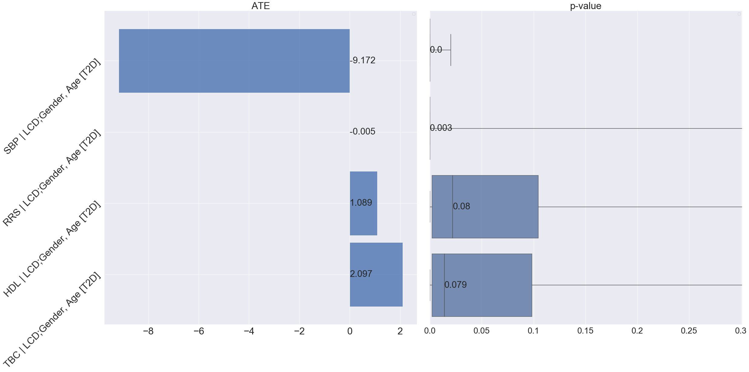
This decomposition can be applied to each permutation in each subsample. The estimates are averaged, yielding an estimate of the indirect effect and corresponding distribution of the p-values. Based on this result, we can assess the indirect effect of LCD on the Reynolds risk score, where the result is provided in Table 3. The negative sign on the indirect effect indicates that, in addition to its direct effect, the LCD lowered Reynolds risk score through the mediator T2D. We report the average ATEs and box plots for the distributions of p-values for other CVD risk factors in Figure 8. It shows that the LCD would also have a significant indirect causal effect on other risk factors of CVD, including a reduction in systolic blood pressure (SBP) and an improvement in good cholesterol (HDL). We found, however, that the LCD would have a significant indirect effect in the form of an increase in serum total cholesterol (TBC).

5 Case Study II: Is Obesity A Significant Risk Factor for T2D and CVD?

5.1 Causal effect of obesity on T2D

Figure 9: Assumed coarse-grained causal graph for the relationship between BMI and T2D, with gender and age as confounders.

Building on the queries in the previous section, we now want to quantify the causal effect of obesity on T2D and CVD ⁴⁴. Consider the counterfactual question,

“What would be the effect on T2D if an individual changes from normal weight to overweight?"

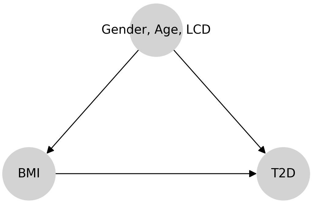
This question cannot be evaluated with a randomized controlled trial, which would require an experimenter to randomly assign individuals to be either obese or of normal weight. Instead, we can attempt to estimate the effect of obesity on T2D from observational data. We make the following assumptions and a specification of the underlying causal structure. First, the BMI is modeled as a categorical variable in this section: normal weight if $\text{BMI}<25$, overweight if $\text{BMI}\in[25,30)$, obese if $\text{BMI}\in[30,35)$), and severely obese if $\text{BMI}\geq 35$. In our analysis, we compare consecutive ordinal levels of obesity pairwise. At each time, we denote the higher level of obesity as 1 (treatment) and the lower level of obesity as 0 (control). Second, similar to the motivating example in Section 2.1, gender is a binary variable and age is an ordinal variable, and the medical outcome T2D is an ordinal variable indicating status at time of reporting: non-diabetics, pre-diabetics, and diabetics. Finally, we assume the causal graph shown in Figure 9, and motivate it by thinking of the following data-generating process: (1) BMI affects the risk of T2D; (2) Gender, age and LCD are unaffected by the BMI level; (3) Gender, age and LCD affect the risk of T2D and the BMI level. Thus gender, age and LCD are confounders of BMI and T2D. (4) Causal sufficiency: there are no hidden confounders. Under these assumptions, we can calculate an estimate of the effect of BMI on T2D, by adjusting for the confounders using the model of potential outcomes in Section 2.3.

Table 4: Average treatment effect of BMI on T2D: $\mathbb{E}[\tau_{5}]$

	Normal weight vs. overweight	Overweight vs. obese	Obese vs. severely obese
ATE	0.477	0.316	0.14
p-value	0.002	0.011	0.196

According to the causal graph in Figure 9, BMI takes the role of a treatment that affects the outcome T2D. To quantify the expected change in T2D if BMI were changed, we need to calculate

$$\mathbb{E}[\tau_{5}(\text{Gender}_{i},\text{Age}_{i},\text{LCD}_{i})],$$

where the potential outcome $\tau_{5}$ is defined as

$$\tau_{5}(\text{Gender}_{i},\text{Age}_{i},\text{LCD}_{i})=\mathbb{E}[\text{T2D}_{i}(\text{BMI}=1)|\text{Gender}_{i},\text{Age}_{i},\text{LCD}_{i}]-\mathbb{E}[\text{T2D}_{i}(\text{BMI}=0)|\text{Gender}_{i},\text{Age}_{i},\text{LCD}_{i}].$$

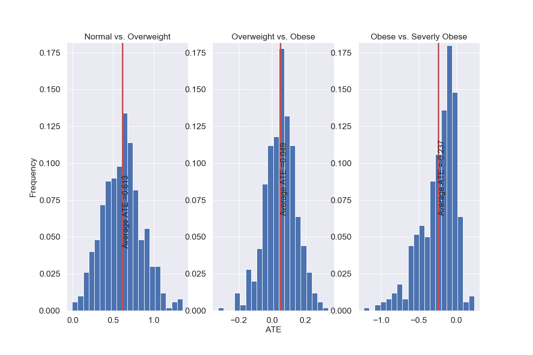
By I-Rand in Algorithm 2, we obtain the mean of ATEs $\mathbb{E}[\tau_{1}]$ over $500$ subsamples and the mean p-value (from the permutation tests) as follows (see, also Figure 10) for all three pairwise differences: (1) changing from normal weight to overweight; (2) changing from overweight to obese; (3) changing from obese to severely obese.

Figure 10: Mean ATE bar plot (left) and p-value box plot (right) for BMI as the treatment. Each row corresponds to a causal diagram: “Outcome $|$ Treatment; Confounders". For example, “SBP $|$ BMI; Gender, Age, T2D" represents the the causal diagram with the systolic blood pressure as the outcome, and the gender, age, T2D as the confounders, and the BMI as the treatment which takes three pairwise comparisons: normal weight vs. overweight (green), overweight vs. obesity (orange), obesity vs. severe obesity (blue).

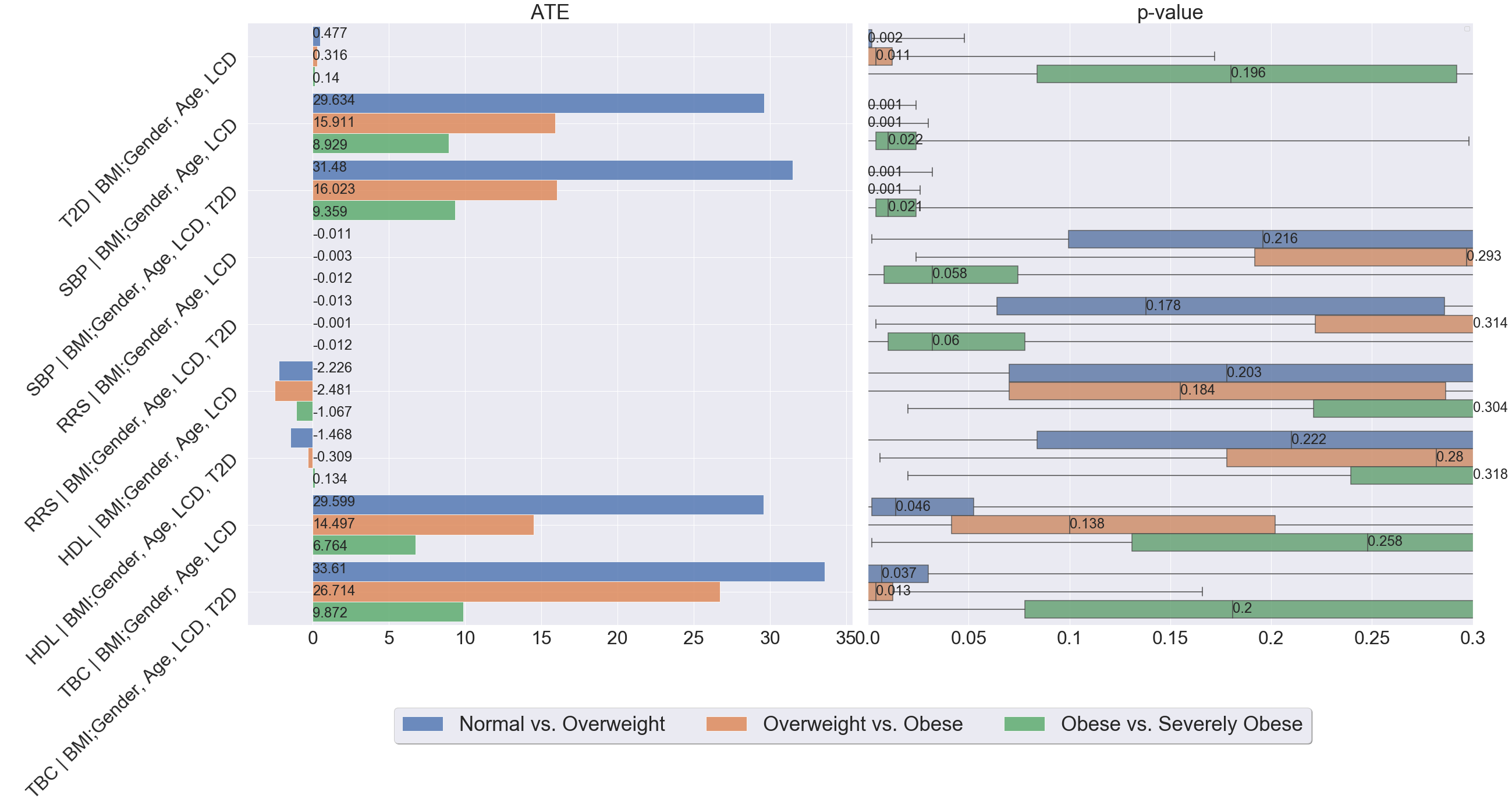
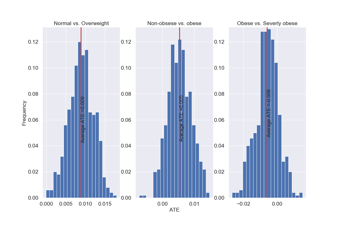
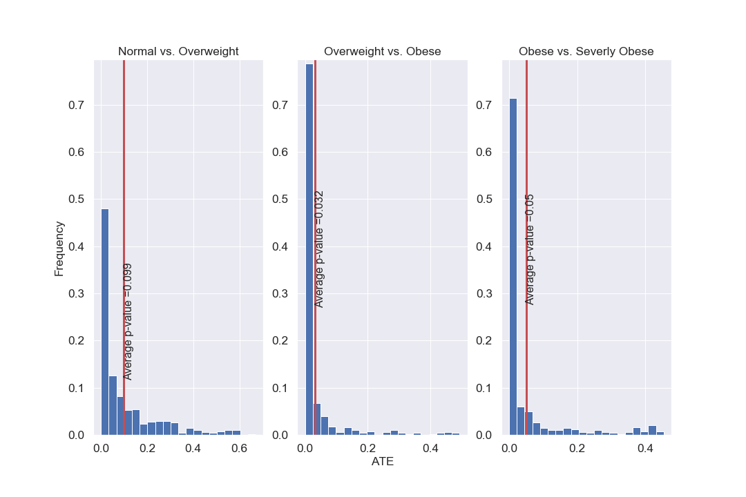
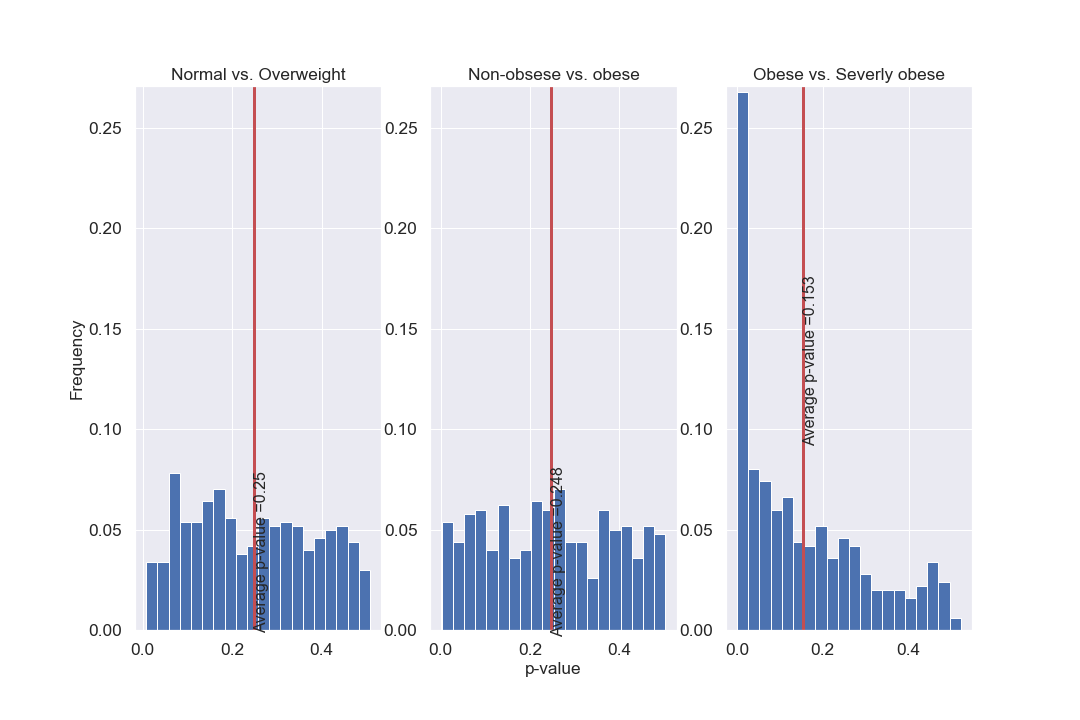
We summarize the results in Table 4, which suggests that the difference of T2D constitutes a causal effect, and changing BMI level from a lower level to a higher level would lead to an increased risk of T2D, where the results are subject to our modelling assumptions. We note that under the null hypothesis of no causal effect, the p-values follow a uniform distribution on $(0,1)$ given sufficiently many subsamples. However, the box plot of p-values in Figure 10, corresponding to the causal graph in Figure 9, shows p-values are concentrated at the origin, which indicates a strong evidence for the alternative hypothesis. In particular, the causal effect of the treatment (normal weight vs. overweight) with p-value $0.002$ is significant under the Bonferroni’s false discovery control at the $0.01$ level. The detailed distributions of ATEs and p-values are provided in Appendix D, which confirms the consistency of these results across subsamples.

5.2 Mediation analysis for the effect of obesity on CVD

We now seek to understand the role of T2D as a mediator of the effect of obesity on CVD risk. As discussed in Section 4.2, this mediation analysis is particularly relevant from the perspective of an individual with both T2D and CVD. We study four well-known risk factors of CVD: systolic blood pressure, serum cholesterol level, high-density lipoprotein, and Reynolds risk score; see, Ridker et al. ²².

5.2.1 Causal graph of T2D as a mediator

Figure 11: Assumed coarse-grained causal graph for the relationship between BMI, T2D, and the outcome CVD. Within this view, T2D acts as a mediator of the effect of BMI on CVD, with the gender, age and LCD as confounders.

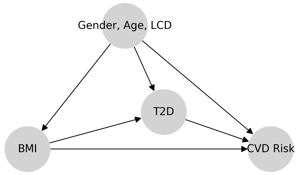
We assume the causal graph in Figure 11, and motivate Figure 11 with the following data-generating process: (1) Choose a BMI level at random; (2) Given a selected BMI level, sample an individual with a T2D status; (3) Conditional on the choice of BMI level and T2D status, sample the medical outcome within a given CVD risk factor. The details are as follows. First, the arrow BMI $\to$ T2D encodes that the distribution of T2D depends on BMI level. This dependence was quantified in Section 5.1. Second, the arrow T2D $\to$ CVD reflects the established knowledge in nutrition science that T2D influences CVD risk ^{41, 5}. Finally, since our model assumes causal sufficiency, and in particular, that T2D is the only mediator in the effect of BMI on CVD risk, the arrow BMI $\to$ CVD represents obesity-specific influences on CVD risk. In addition to the causal graph in Figure 11, we assume there are no hidden confounders. Given these assumptions, we see that BMI causally influences CVD risk along two different paths: a path BMI $\to$ CVD, giving rise to a direct effect, and a path BMI $\to$ T2D $\to$ CVD mediated by T2D, giving rise to an indirect effect. Note that the direct effect of BMI on CVD is likely mediated by additional variables that are subsumed in BMI $\to$ CVD Risk. We discuss this point further in Section 6. In mediation analysis, the goal is to quantify direct and indirect effects. We start with the total effect and then formulate the direct and indirect effects by allowing the treatment to propagate along one path while controlling the other path.

5.2.2 Total effect of BMI on CVD

Given the causal assumptions in the previous section, the first measure of interest is the total causal effect of obesity on CVD, i.e., the answer to the following question:

“What would be the effect on CVD if an individual changes from normal weight to overweight?"

As we did in Section 5.1, we formulate the answer using the ATE:

$$\mathbb{E}[\tau_{6}(\text{Gender}_{i},\text{Age}_{i},\text{LCD}_{i})],$$

where the potential outcome $\tau_{6}$ is defined as

$$\tau_{6}(\text{Gender}_{i},\text{Age}_{i},\text{LCD}_{i})=\mathbb{E}[\text{CVD}_{i}(\text{BMI}=1)|\text{Gender}_{i},\text{Age}_{i},\text{LCD}_{i}]-\mathbb{E}[\text{CVD}_{i}(\text{BMI}=0)|\text{Gender}_{i},\text{Age}_{i},\text{LCD}_{i}].$$

We now give a detailed result for one of the CVD risk factors, namely the systolic blood pressure, where the description and the summary statistics are deferred to Appendix C. It is known that increasing systolic blood pressure significantly increases the risk of CVD (e.g., Bundy et al. ⁴⁵). By the proposed I-Rand with $500$ subsamples and the corresponding permutation test for each subsample, we obtain the mean of ATEs $\mathbb{E}[\tau_{6}]$ given in Table 5.

Table 5: Mediation analysis for the effect of BMI on SBP

	Normal weight vs. overweight	Overweight vs. obese	Obese vs. severely obese
Total effect $\mathbb{E}[\tau_{6}]$ (p-value)	29.634 (0.001)	15.911 (0.001)	8.929 (0.022)
Direct effect $\mathbb{E}[\tau_{7}]$ (p-value)	31.48 (0.001)	16.023 (0.001)	9.359 (0.021)
Indirect effect $\mathbb{E}[\tau_{8}]$ (p-value)	-1.846 (0.112)	-0.112 (0.146)	-0.43 (0.231)

The results show that an individual changing from normal weight to overweight would significantly lead to an increase in systolic blood pressure. In contrast, the box plot of p-values in Figure 10 indicates only weak evidence that changing BMI would have a causal effect on other risk factors of CVD including serum total cholesterol (TBC), high-density lipoprotein (HDL), and Reynolds risk score (RSS). The observation is also supported by distributions of ATEs and p-values in Appendix D. The failure to reject the null hypothesis may also be due to unobserved confounders such as genetic information, smoking, and stress levels.

5.2.3 Direct effect of BMI on CVD

We now study the natural direct effect (see, Pearl ⁴³) of obesity on CVD risk in the context of the following hypothetical question:

“For an individual of normal weight, how would a weight gain affect the risk of CVD?"

We are asking what would happen if the treatment, BMI, were to change, but that change did not affect the distribution of the mediator, T2D. In that case, the change in treatment would be propagated only along the direct path BMI $\to$ CVD in Figure 11. To disable all but the direct path, we need to stratify by T2D. This closes the indirect path BMI $\to$ T2D $\to$ CVD. But in so doing, it opens the path BMI $\to$ T2D $\leftarrow$ (Gender, Age, LCD) $\to$ CVD since T2D is a collider in Figure 11. If we control for (Gender, Age, LCD) as well, we close the direct path, and therefore any correlation remaining must be due to the direct path BMI $\to$ CVD.

To quantify the expected change in T2D if BMI were changed, we need to calculate

$$\mathbb{E}[\tau_{7}(\text{Gender}_{i},\text{Age}_{i},\text{LCD}_{i},\text{T2D})],$$

and where the potential outcome $\tau_{7}$ is defined as follows:

$$\tau_{7}(\text{Gender}_{i},\text{Age}_{i},\text{LCD}_{i},\text{T2D}_{i}) =\mathbb{E}[\text{CVD}_{i}(\text{BMI}=1)|\text{Gender}_{i},\text{Age}_{i},\text{LCD}_{i},\text{T2D}(\text{BMI}=0)]$$

$$\quad\quad-\mathbb{E}[\text{CVD}_{i}(\text{BMI}=0)|\text{Gender}_{i},\text{Age}_{i},\text{LCD}_{i}].$$

The symbol $\text{T2D}(\text{BMI}=0)$ refers to the counterfactual distribution of T2D given that the value of BMI is 0, and the expectations are taken over the corresponding interventional (i.e., $\text{BMI}=0,1$) and counterfactual (i.e., $\text{T2D}(\text{BMI}=0)$) distributions. Hence, $\tau_{7}$ defines the influence that is not mediated by T2D in the sense that it quantifies the sensitivity of the CVD to changes in BMI while T2D is held fixed, as illustrated in Figure 11. By I-Rand algorithm, we obtain mean ATEs $\mathbb{E}[\tau_{7}]$ with $500$ subsamples and the mean p-value of permutation tests for systolic blood pressure in Table 5. See, also Figure 10 for other CVD risk factors. In addition to the summary statistics shown above, we provide the distributions of ATEs and p-values of the subsampling in Appendix D.4. We find, for example, that a change from normal weight to overweight would lead to a increase in systolic blood pressure of $31.48$ mmHg on average (see Appendix C for summary statistics of systolic blood pressure). The direct effect in this example represents a stable biological relationship that, different from the total effect, is robust to T2D and any cause of high systolic blood pressure that is mediated via T2D.

5.2.4 Indirect effect of BMI on CVD

We conclude this section by studying the indirect effect in the context that

“How would the CVD risk of a normal weight individual be if his / her T2D status had instead following the T2D distribution of overweight individuals?"

The answer is formulated by

$$\mathbb{E}[\tau_{8}(\text{Gender}_{i},\text{Age}_{i},\text{LCD}_{i},,\text{T2D})],$$

where the potential outcome $\tau_{8}$ is defined

$$\tau_{8}(\text{Gender}_{i},\text{Age}_{i}) =\mathbb{E}[\text{CVD}_{i}(\text{BMI}=0)|\text{Gender}_{i},\text{Age}_{i},,\text{LCD}_{i}\text{T2D}(\text{BMI}=1)]$$

$$\quad\quad-\mathbb{E}[\text{CVD}_{i}(\text{BMI}=0)|\text{Gender}_{i},\text{Age}_{i},\text{LCD}_{i}].$$

Under our assumptions, any changes that occur in an individual’s CVD risk are attributed to BMI-induced T2D and not to the BMI itself. The indirect effect of the treatment is the change of CVD risk obtained by keeping the BMI of each individual fixed and setting the distribution of T2D to the level obtained under treatment.

Figure 12: Indirect Effect: Mean ATE bar plot (left) and p-values box plot (right) for the indirect effect of BMI on CVD risk factors with age and gender as confounders and T2D as a mediator. Each row corresponds to a causal diagram: “Outcome $|$ Treatment; Confounders [Mediator]”. For example, “SBP $|$ BMI; Gender, Age, [T2D]” represents the causal diagram with the systolic blood pressure as the outcome, gender and age as the confounders, T2D as the mediator, and BMI as the treatment.

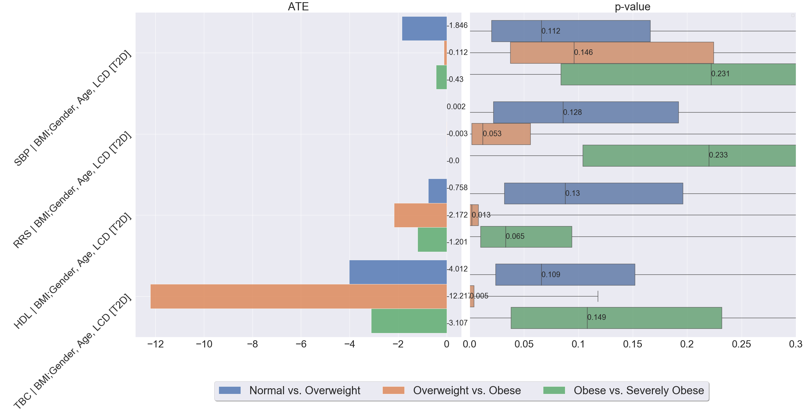
Consider a linear model in which there is no interaction between treatment and mediator. This yields the decomposition (11) and the indirect effect of BMI on the systolic blood pressure given in Table 5. We report the average ATEs and box plots for the distributions of p-values for other CVD risk factors in Figure 12 . We find that changing only the distribution of T2D that results from an increase in BMI from normal weight to overweight would lead to a decrease in systolic blood pressure of about $1.848$ mmHg on average. Notably, the sign of this indirect effect is opposite to the sign of the corresponding direct effect, which suggests that indirect and direct effects tend to offset one another. There are several possible explanations for this. For example, the offset may be due to missing BMI data, which results in selection bias. Further discussion of selection bias is in Section 6. Another possible explanation is the obesity paradox given the comorbidity conditions (see, e.g., Uretsky et al. ⁴⁶ and Lavie et al. ¹⁸) that overweight people may have a better prognosis, possibly because of the medication or overweight individuals having lower systemic vascular resistance compared to leaner hypertensive individuals.

6 Discussion on Assumptions and Models

We assume the causal relationships between variables of demographics, obesity, T2D, and CVD to be captured by causal graphs in the previous sections, which correspond to different nutrition-related questions. These causal graphs constitute a coarse-grained view, which neglects many potentially important risk factors. A strength of this coarse-grained approach is that it allows for quantitative reasoning about different causal effects including total, direct, and indirect effects in situations where the data do not allow a more fine-grained analysis. In the following, we discuss assumptions and limitations of our approach and point out some future directions.

6.1 Selection bias

The data we considered concerns only those patients who are from the Norwood general practice surgery in England and has opted to follow LCD by 2019 ². We can introduce an additional variable $V$ with $V=1$ meaning that an individual who is from the Norwood general practice surgery and follows LCD by 2019 and $V=0$ otherwise. In that case, our analysis is always conditioned on $V=1$. If the individual who follows LCD is randomly sampled from the population of Norwood general practice surgery with 9,800 patients, the implicit conditioning on $V=1$ would not introduce bias to an inference for the larger population. However, samples are generally not collected randomly. In particular, age and health conditions are causal factors on the participation in the LCD program, i.e., age $\to V$ and health condition $\to V$ and through self-selection. Moreover, due to the possible speciality and reputation of the LCD program, T2D$\to V$, CVD$\to V$. Finally, there may be complex interactions between office visit and T2D or CVD, where the process involves the feedback $V\to$ T2D and $V\to$ CVD. The fact that we consider only individuals who participate in the LCD program while the visit itself depends on multiple other factors inevitably leads to the problem of selection bias. Several approaches have been developed to decrease this bias under certain conditions; see, e.g., Bareinboim and Tian ⁴⁷, Bareinboim and Pearl ⁴⁸.

6.2 Unobserved confounders

An important assumption upon which relies our estimation of the causal effect, is the absence of hidden confounders, i.e., we assume that gender and age are the only confounders. In particular, it is the basis of our estimates of the direct and indirect effects. It may be possible to relax the absence of hidden confounders depending on the availability of experimental data. See Pearl ⁴³ for further discussion.

6.3 Additional mediators

In our coarse-grained view, the arrows possibly subsume many other potentially important risk factors within the causal paths. For example, the strength of the effect BMI $\to$ T2D in Section 2.1 is estimated without consideration of mediators.

6.4 Model selection

In this section, we compare the proposed I-Rand with the method of difference-in-differences (DD; e.g., Angrist and Pischke ¹⁶), which studies the impact of the differential effect of a treatment on a “treatment group" versus a “control group". Then we discuss some generalizations of the models used for analysis in the previous sections. The following analysis explores the impact of difference in treatment on difference in outcome (DD). For a given variable, we calculate the difference as the value on the second visit minus the value on the first visit. In our analysis, we set confounders (e.g., age and gender) to the values recorded at the first visits. We note two main differences between I-Rand and DD. First, when the LCD is the treatment, all individuals are LCD-takers and there is no control group. The I-Rand creates a control group by subsampling, while difference-in-differences relies on the null hypothesis of “no effect.” Second, when BMI is the treatment, I-Rand subsamples one of the two observations for each individual to avoid two types of unintended treatments. In DD, such subsampling is unnecessary since we have one observation for each individual. We perform two experiments: a decrease in BMI (i.e., $\Delta\text{BMI}<0$), or a change in BMI in excess of a threshold (e.g., $\Delta\text{BMI}$ $<\text{median of }|\Delta\text{BMI}_{i}|$). The latter choice of treatment splits the data into two equally-sized subgroups of treatment and control, and it is more robust than the first choice of treatment since the BMI of almost all individuals decreased between visits. For BMI with a median threshold, the causal effect for individual $i$ has the usual estimation formula, i.e., ATE $=\mathbb{E}|\tau(X_{i})]$, where $\tau(X_{i})=\mathbb{E}[Y_{i}(1)|X_{i}]-\mathbb{E}[Y_{i}(0)|X_{i}]$. In the case of LCD and decrease of BMI, the causal effect reduces to $\tau(X_{i})=\mathbb{E}[Y_{i}(1)|X_{i}]$. Note that the design of the experiment however, breaches the non-zero probability of receiving treatment assumption, i.e., $0<P(T=1|X)<1$, which is required by the causal effect estimation. As a matter of fact, all individuals are treatment-takers between the two observation dates. Hence, we add a hypothetical control group that does not take the treatment and has a $0$ valued outcome. To estimate the causal effect for the latter that is applicable to permutation analysis, we implement Algorithm 3 for difference-in-differences analysis.

1:Input: Observed data of confounders, treatment and outcome $(X_{i,t},T_{i,t},Y_{i,t})$ where $i$ is the individual’s ID and $t$ is the state.

2:Create the “treatment” difference-in-differences matrix with $T_{i,1}=T_{i,t=1}-T_{i,t=0}$, $Y_{i,1}=Y_{i,t=1}-Y_{i,t=0}$, $X_{i,1}=X_{i,t=0}$. Its “control” image with the following attributes: $T_{i,0}=0$, $Y_{i,t=0}=0$, $X_{i,0}=X_{i,t=0}$. Form the difference-in-differences matrix as the concatenation of the two.

3:Calculate ATE by the matching method over the concatenated matrix. Here, the estimation of the ATE leads to $\mathbb{E}[Y_{i}(1)|X_{i}]-\mathbf{0}$ since the control set consists of only $0$ valued outcomes. In the permutation analysis on the other hand, the estimation results in a difference of the two usual quantities.

4:Perform the permutation analysis: for $s=1,2,\ldots,S$ do

5:  Sample a binary vector of length $N$, where the index is the individual’s ID and the value is the state (sampling without replacement). Selecting the corresponding subsample $s$ as the shuffled vector of treatment. Note that the shuffling performed is equivalent to assigning each individual the treatment with probability 1/2 ($N$ independent Bernoulli variables with parameter $p=1/2$). This is a strong assumption that needs to be supported by data. However, this choice is consistent with our I-Rand algorithm and can further be adjusted to a better choice of $p$;

6:  Calculate $ATE^{(s)}$ for the shuffle $s$ of the treatment.

7:end for

8:Calculate the p-value$=\frac{1}{S}\sum_{s=1}^{S}\mathbbm{1}_{ATE^{(s)}>(\text{resp. }<)ATE}$ for the one-tailed test for the null hypothesis of no treatment effect.

9:Output: ATE and p-value.

Algorithm 3 Difference-in-difference with data re-organization of two-point time-series without control group

Figure 13: Bar plot of ATE for LCD as the treatment for the difference-in-differences analysis without threshold (we omit the p-values as they are all under a 1% significance level). Each row corresponds to a causal diagram:“Outcome $|$ Treatment; Confounders”. For example, “SBP|LCD; Gender, Age, BMI” represents the causal diagram with the systolic blood pressure as the outcome, and gender, age, BMI as the confounders, and LCD as the treatment.

Figure 14: Bar plot of ATE for BMI as the treatment for difference-in-differences analysis without threshold (we omit the p-values as they are all under a 1% significance level). Each row corresponds to a causal diagram:“Outcome $|$ Treatment; Confounders”. For example, “SBP $|$ BMI; Gender, Age” represents the causal diagram with the systolic blood pressure as outcome, gender and age as confounders, and BMI as treatment.

Figure 15: Bar plot of ATE (left) and p-value (right) for BMI as the treatment for the difference-in-differences analysis with threshold (median). Each row corresponds to a causal diagram:“Outcome $|$ Treatment; Confounders”. For example, “SBP $|$ BMI; Gender, Age” represents the causal diagram with the systolic blood pressure as the outcome, and gender, age as the confounders, and BMI as the treatment.

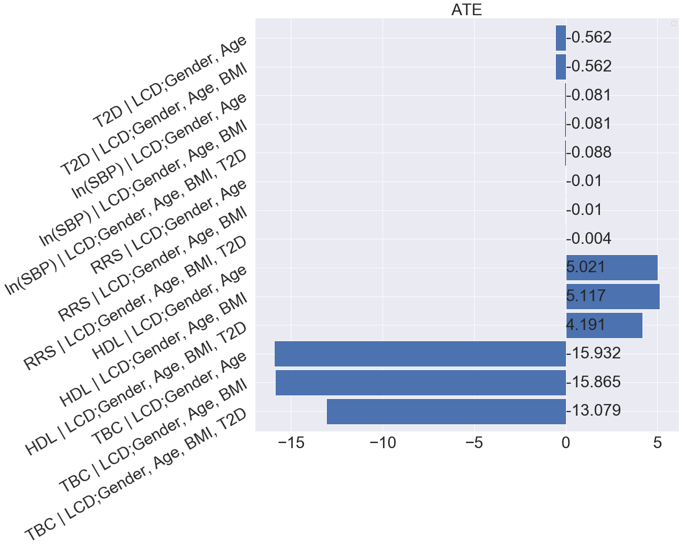
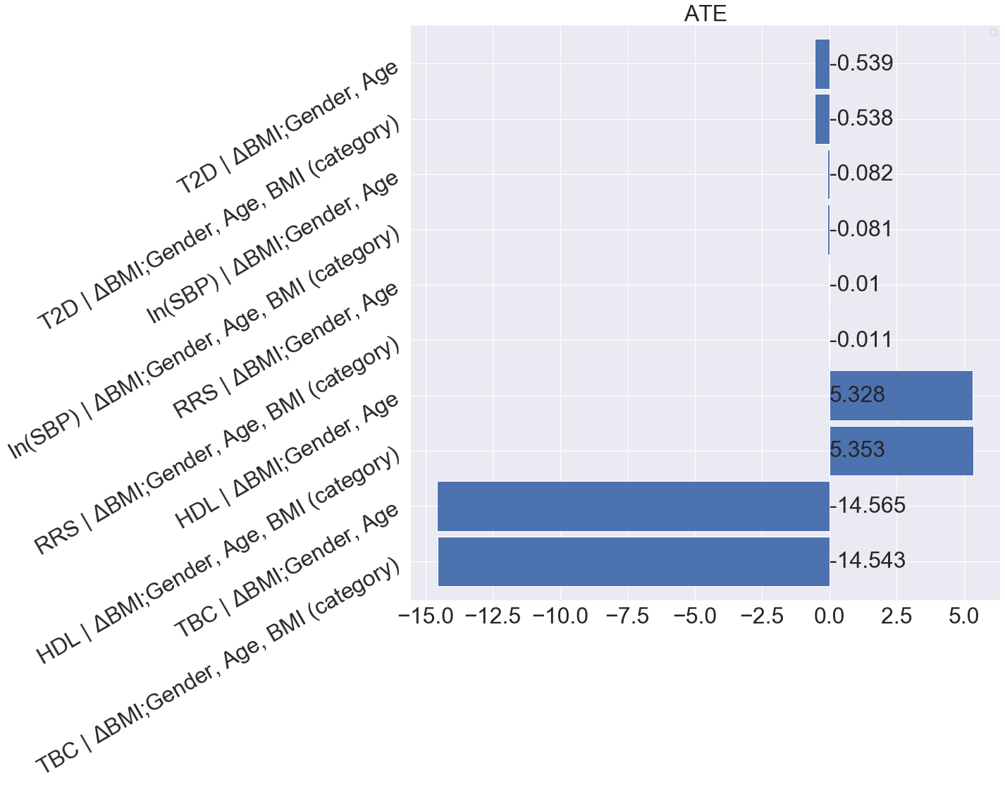
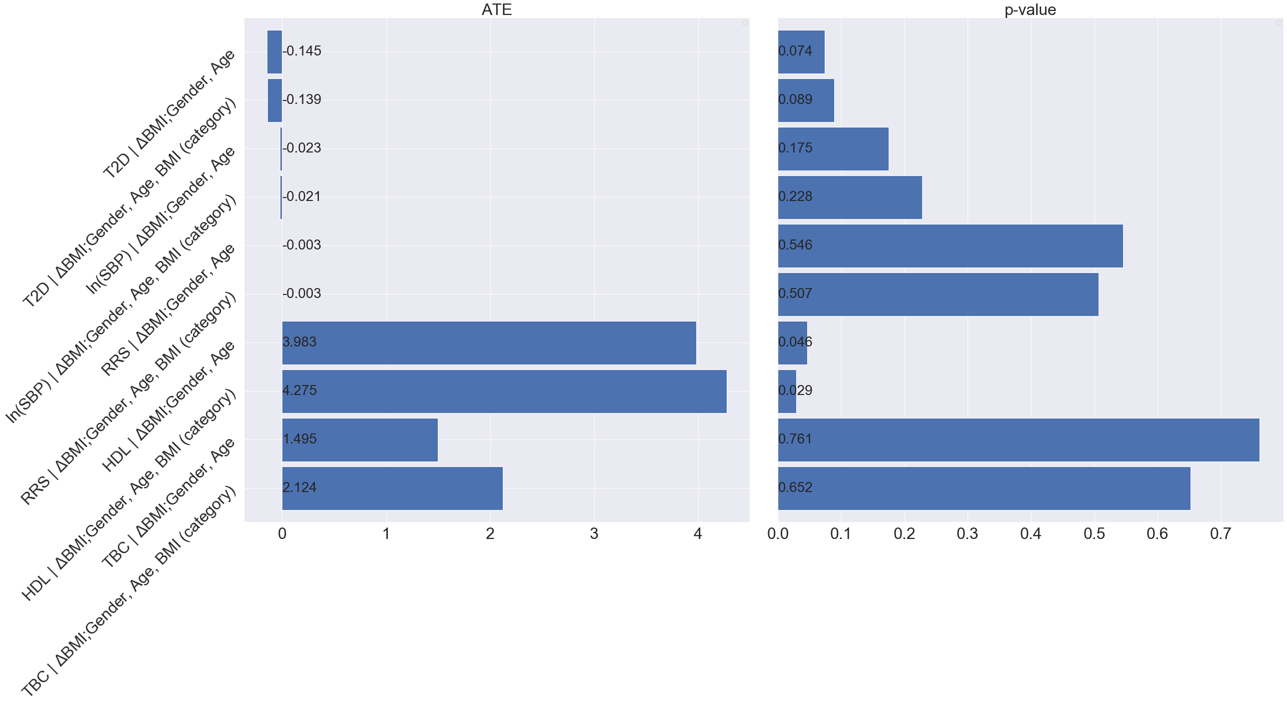
We summarize the results in Figures 13, 14, and 15. For a change in diet (i.e., $\Delta\text{LCD}=1$), we find that LCD diet significantly impacts the change in T2D status and CVD risk factors. The same applies to the first choice of treatment for BMI (i.e., $\Delta$ BMI $<0$). For the second choice of treatment for BMI (i.e., $\Delta$ BMI $<\text{Threshold}$), we find that a change in BMI has a significant causal effect on a change in T2D even when controlling for the BMI categories. Moreover, a decrease in BMI leads to an increase in HDL (ATE$=3.983$, p-value$<4.6\%$ without controlling for BMI categories and ATE$=4.275$, p-value$<2.9\%$ when controlling for BMI categories).

The limitation of the difference-in-differences in our dataset is that we do not have enough data for longitudinal analysis. As a result, variance across samples (noise) could be much larger than the variance within samples (signal). On the other hand, the results based on the difference-in-differences method with only two time points are always subject to biases (e.g., Raudenbush ⁴⁹).

There are different ways to generalize our linear models to nonlinear models. For example, it could be of interest to ask whether or not BMI above a certain threshold has a causal effect on CVD or T2D. Moreover, the linear models we used in this article cannot represent interactions among variables. It could also be of interest to assess the direct and indirect effects allowing for interactions between treatments and mediators ⁴³.

Appendix A Matching Methods

A.1 Distance measure based on propensity score

We need to determine which confounders to include for matching and to combine those variables into one measure. Under the strong ignorability assumption, it is necessary to include all variables known to be related to both treatment assignment and the outcome in the matching procedure ^{50, 25}. There is little cost to including variables that are not associated with treatment assignment. However, excluding a potentially important confounder can yield a large bias. In the other direction, variables such as colliders and mediators that may have been affected by the treatment should be excluding from the matching process, and should be used instead in the analysis model for outcomes (see, Greenland ⁵¹).

The propensity score, a popular measure to combine confounders, is defined for each individual $i$ as the probability of receiving the treatment, given the observed confounders ²⁷:

$$e_{i}(X_{i})=\mathbb{P}(T_{i}=1|X_{i}).$$

The propensity score has two well-known properties. First, a propensity score is a balancing score in the sense that at any level of the propensity score, the distributions of the confounders defining the propensity score in the treated and control groups are the same. Second, the treatment assignment is ignorable given the propensity score if treatment assignment is ignorable given the confounders. Hence, it is reasonable to match individuals on the basis of propensity score rather than the vector of multivariate confounders.

These properties imply that the difference in means for the outcomes between treated and control individuals with a particular propensity score value is an unbiased estimate of the treatment effect at that propensity score value. The distance between individuals $i$ and $j$ through the propensity score is $D_{ij}=|e_{i}-e_{j}|$. In practice, propensity scores are unknown and we use logistic regression to estimate $e_{i}$s for the case studies in Sections 5 and 4.

A.2 Propensity score matching

We apply the propensity score matching algorithm for our case studies in Sections 5 and 4. The simple weighted difference in means estimate for the ATE is given in the step 2 of the algorithm in Section 2.3.

We use matching with replacement to minimize the propensity score distance between the matched control individuals and the treatment individuals. This reduces bias, even if an individual in the control group is matched more than once. As a comparison, matching without replacement is sensitive to the order in which individuals are matched. This method may force us to match individuals whose propensity scores are far apart, leading to an increase in bias. Further, We also use the single-nearest-neighbor matching, which selects a single individual in the control group whose propensity scores are closest to those of the treated individual. Single-nearest-neighbor matching can be extended to $k\geq 1$ nearest-neighbors.

In addition to the simple weighted difference in means for estimating the treatment effect in the algorithm in Section 2.3, one can also use a weighted regression, which takes account of the number of times a control is matched (see, e.g., Dehejia and Wahba ⁵².)

A.3 Model diagnosis

The diagnosis of the quality of the resulting matched samples is an important step in using matching methods. In particular, we need to assess the covariate balance in terms of the similarity of the empirical distributions of the full set of confounders in the matched treated and control groups. Ideally, we want the empirical distribution of $X_{T=1}$ in the treatment group is the same as the empirical distribution of $X_{T=0}$ in control treatment group . That is, the treatment is unrelated to the confounders.

In our case studies in Sections 5 and 4, we apply the standardized difference in means as a balance measure: $(\bar{X}_{T=1}-\bar{X}_{T=0})/\sigma_{T=1}$, where $\bar{X}_{T=1}$ and $\bar{X}_{T=0}$ are sample means of the treatment and control groups, and $\sigma_{T=1}$ is the sample standard deviation for the treatment group. We calculate the standardized difference in means for each covariate and use the $(\bar{X}_{T=1}-\bar{X}_{T=0})/\sigma_{t}<0.25$ as a criteria to check that the matching gives balanced samples (see, e.g., Rubin ⁵³).

Appendix B Proofs

B.1 Proof of Theorem 3.1

Proof B.1.

We claim that under the LCD-like treatment design (3), it is not possible to obtain an accurate estimate of the treatment effect (6) if the parametric functional forms of $f(\cdot)$ and $g(\cdot)$ in (2) are unknown. This claim is explained as follows. Under the null hypothesis that there is no trend in the control group $\{i|T_{i}(t=1)=0,T_{i}(t=0)=0\}$, i.e.,

$$\mathbb{E}_{X}[\mathbb{E}[Y_{i}(t=1)|T_{i}(t=1)=0,T_{i}(t=0)=0,X]]=\mathbb{E}_{X}[\mathbb{E}[Y_{i}(t=0)|T_{i}(t=1)=0,T_{i}(t=0)=0,X]],$$ (12)

then the difference-in-differences leads to an estimate to the following effect:

$$\mathbb{E}_{X}[\mathbb{E}[Y_{i}(t=1)-Y_{i}(t=0)|T_{i}(t=1)=1,T_{i}(t=0)=0,X]]$$ (13)

$$=f(1)-f(0)+\mathbb{E}[g(X_{i}(t=1))]-\mathbb{E}[g(X_{i}(t=0))].$$

Here $f(1)-f(0)$ corresponds to the treatment effect in (6) and $\mathbb{E}[g(X_{i,1})]-\mathbb{E}[g(X_{i,0})]$ is the nuisance effect from the confounder. If the parametric functional forms of $f(\cdot)$ or $g(\cdot)$ is unknown, it is easy to show that for $g^{\prime}(\cdot)\equiv 2g(\cdot)$, the treatment effect $f^{\prime}(1)-f^{\prime}(0)$ defined as follows satisfies (13):

$$f^{\prime}(1)-f^{\prime}(0) \equiv\mathbb{E}_{X}[\mathbb{E}[Y_{i}(t=1)-Y_{i}(t=0)|T_{i}(t=1)=1,T_{i}(t=0)=0,X]]$$

$$\quad-\{\mathbb{E}[g^{\prime}(X_{i}(t=1))]-\mathbb{E}[g^{\prime}(X_{i}(t=0))]\}.$$

However, $f^{\prime}(1)-f^{\prime}(0)\neq f(1)-f(0)$. Hence, the treatment effect $f(1)-f(0)$ is unidentiable using difference-in-differences under the two-point structure (3).

B.2 Multiple treatment versions

Theorem B.2.

Suppose that for each individual, there is a fixed version that would have been received, had the individual been given $T\in\{0,1\}$. Then if Figure 16 is a causal graph, the average treatment effect is equivalent to

$$\text{ATE}^{*}\equiv\mathbb{E}_{X}[\mathbb{E}[Y|T=1,X]]-\mathbb{E}_{X}[\mathbb{E}[Y|T=0,X]].$$ (14)

The I-Rand Algorithm 2 gives an unbiased estimate of $\text{ATE}^{*}$ in (14) if the estimator $\text{ATE}^{(m)}$ in (1) is unbiased for ATE.

Figure 16: Causal graph illustrating relationship between treatment $T$, version of $T$, outcome $Y$, and $X$ consists of observed and unobserved confounders.

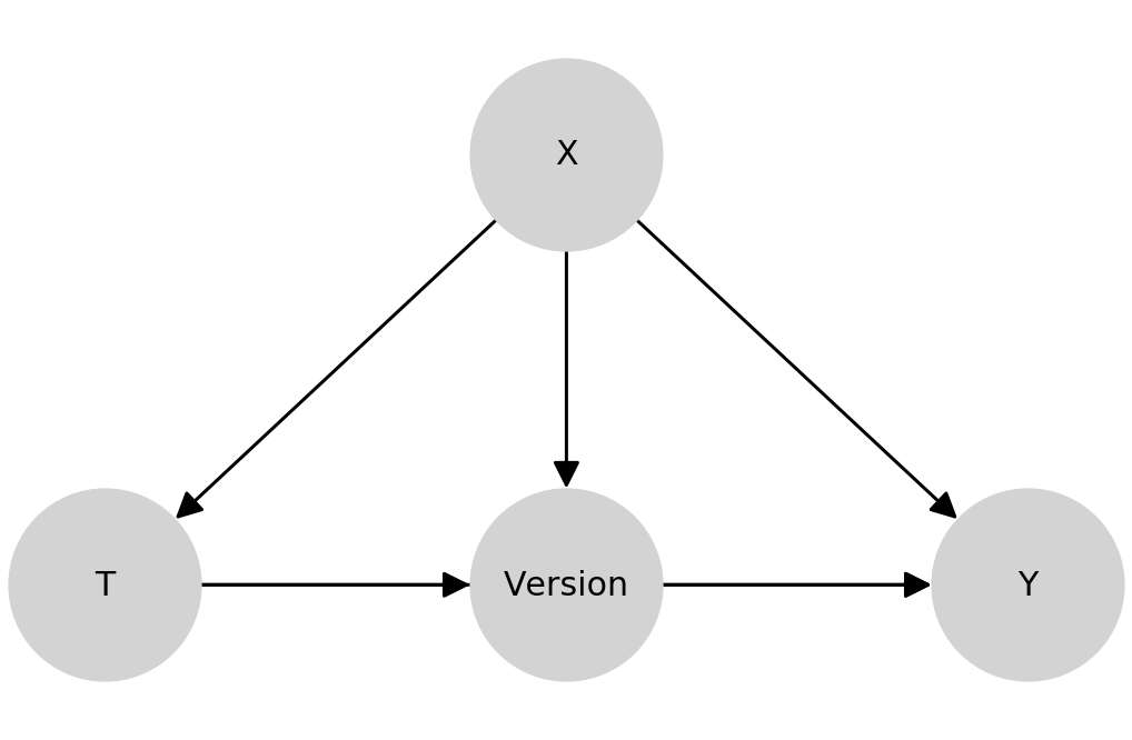
Proof B.3.

Since there is a fixed version of treatment that an individual would have been received if the individual has been given $T\in\{0,1\}$, we have

$$\mathbb{E}[Y(T)]=\mathbb{E}_{X}[\mathbb{E}[Y(T)|X]]=\mathbb{E}_{X}[\mathbb{E}[Y(T)|T,X]].$$

where the last step is due to the fact that given Figure 16, $T$ is ignorable relative to outcome $Y$, conditional on $X$ ³¹. Denote by $K^{T}(T)$ the counterfactual variable of which version of treatment that an individual would have been received if the individual has been given $T\in\{0,1\}$. Then

$$\mathbb{E}_{X}[\mathbb{E}[Y(T)|T,X]] =\mathbb{E}_{X}[\mathbb{E}[Y(T,K^{T}(T))|T,X]]$$

$$=\mathbb{E}_{k^{T},X}[\mathbb{E}[Y(T,k^{T})|T,K^{T}(T)=k^{T},X]]$$

$$=\mathbb{E}_{k^{T},X}[\mathbb{E}[Y(T,k^{T})|T,K^{T}=k^{T},X]]$$

$$=\mathbb{E}_{k^{T},X}[\mathbb{E}[Y|T,K^{T}=k^{T},X]]$$

$$=\mathbb{E}_{X}[\mathbb{E}[Y|T,X]].$$

where the third step is by the assumption that there is a fixed version of treatment that an individual would have been received, and the third step is by the consistency for $Y$. Therefore, $\mathbb{E}[Y(T)]=\mathbb{E}_{X}[\mathbb{E}[Y|T,X]]$ and we obtain the desired the average treatment effect

$$\mathbb{E}_{X}[\mathbb{E}[Y|T=1,X]]-\mathbb{E}_{X}[\mathbb{E}[Y|T=0,X]].$$

Suppose that $X=(X_{1},X_{2})$, where $X_{1}$ consists of observed confounders and $X_{2}$ represents unobserved confounders. Then

$$\mathbb{E}_{X}[\mathbb{E}[Y|T=1,X]]-\mathbb{E}_{X}[\mathbb{E}[Y|T=0,X]]=\sum_{x_{2}}\text{ATE}(X_{2}=x_{2})\mathbb{P}(X_{2}=x_{2}).$$

where

$$\text{ATE}(X_{2}=x_{2})=\mathbb{E}_{X_{1}}[\mathbb{E}[Y|T=1,X_{1},X_{2}=x_{2}]]-\mathbb{E}_{X_{1}}[\mathbb{E}[Y|T=0,X_{1},X_{2}=x_{2}]].$$

By the sampling strategy of the I-Rand estimator (1) yields that $\mathbb{P}(X_{2}=x_{2})=2^{-N}$ and $\text{ATE}^{(m)}$ is a matching method estimator for $\text{ATE}(X_{2}=x_{2})$. This completes the proof.

Appendix C Variables Definition and Summary Statistics of Data Used in the Paper

		count	mean	std	min	25%	50%	75%	max
LCD	Variable
	Gender	256	0.590	0.493	0.000	0.000	1.000	1.000	1.000
	Age	256	61.574	12.111	23.000	53.000	60.000	71.000	91.000
	Height	75	1.706	0.092	1.473	1.625	1.720	1.770	1.900
	Weight	251	96.160	18.621	55.300	83.700	95.000	107.000	159.000
	BMI	66	33.887	6.071	21.660	29.890	33.495	36.980	57.100
0	T2D	256	1.281	0.811	0.000	1.000	2.000	2.000	2.000
	HbA1c/ mmol/mol	202	61.376	20.652	37.000	45.000	54.500	71.000	135.000
	TBC	176	5.314	1.302	2.500	4.385	5.200	6.225	9.300
	HDL	195	1.280	0.421	0.600	1.000	1.200	1.450	3.500
	SBP	171	143.503	15.476	114.000	132.000	142.000	152.000	223.000
	Gender	256	0.590	0.493	0.000	0.000	1.000	1.000	1.000
	Age	256	63.424	12.387	23.167	54.750	62.750	73.500	91.500
	Height	75	1.706	0.092	1.473	1.625	1.720	1.770	1.900
	Weight	251	87.070	17.352	51.000	75.000	84.400	97.100	140.000
	BMI	65	30.356	5.923	19.240	27.040	29.270	32.470	53.620
1	T2D	256	0.719	0.867	0.000	0.000	0.000	2.000	2.000
	HbA1c/ mmol/mol	201	45.925	9.319	32.000	40.000	43.000	50.000	84.000
	TBC	174	4.892	1.247	2.400	4.025	4.700	5.700	8.800
	HDL	189	1.413	0.542	0.700	1.090	1.340	1.610	4.900
	SBP	170	132.100	11.021	108.000	125.000	132.000	139.500	170.000
	months	256	22.199	17.456	1.000	8.000	19.000	32.000	84.000

Table 6: Summary statistics of variables collected in the study. LCD=0 corresponds to data collected at the first visit and LCD=1 for data collected at the second visit.

Gender: a binary variable with “female”$=0$ and “male” $=1$.
Age: the age of the participants at their visit.
BMI: the body mass index of the participants. Here BMI is defined as the ratio of the weight squared height. We note that although recent studies on nutrition suggest that different obesity metrics can lead to different relationships between obesity to CVD risk, the consensus is that compared to BMI measures the more refined modalities (e.g., waist circumference, waist-to-hip ratio, waist-to-height ratio) do not add significantly to the BMI assessment from a clinical perspective ⁵⁴.
T2D: a three-states variable to inform of the type-2 diabetes status; 0 for non-diabetic, 1 for pre-diabetic and 2 for diabetic.
HbA1c: the glycated haemoglobin of the participants. It develops when haemoglobi, a protein within red blood cells that carries oxygen throughout the body, joins with glucose in the blood, becoming ‘glycated’. This measure allows to determine the T2D status.
LCD: a binary variable which equals to $1$ only if the participant is suggested to follow a low-carbohydrate diet.
TBC: the total blood cholesterol level of the participants. It is a measurement of certain elements in the blood, including the amount of high- and low-density lipoprotein cholesterol (HDL and LDL) in a person’s blood.
HDL: the high-density lipoprotein cholesterol of the participants. The HDL is the well-behaved "good cholesterol." This friendly scavenger cruises the bloodstream. As it does, it removes harmful “bad" cholesterol from where it doesn’t belong. A high HDL level reduces the risk for heart disease.
SBP: the systolic blood pressure of the participants. The SBP indicates how much pressure the blood is exerting against your artery walls when the heart beats. It is one of the CVD risk factors used to calculate the Reynolds risk score.
Months: the number of months between the two visits of participants to the clinic (end date – start date).

Appendix D Supplementary Numerical Results

D.1 Treatment effect of LCD on T2D

We provide details on assessing the significance of the reduction of the risk of T2D due to the LCD using the I-Rand algorithm, where the causal diagram is shown in Figure 1. We show the distribution of ATEs for the subsampling step in Figure 17 and the distribution of the p-value from the permutation test under the null hypothesis of no causal effect (ATE = 0) in Figure 18. The distributions confirm the consistency of these results across the subsamples.

Figure 17: Distribution of the ATE of the LCD on T2D in Figure 1. The results are based on 500 subsamples.

Figure 18: Distribution of p-values of the ATE of the LCD on T2D in Figure 1. The results are based on 500 subsamples.

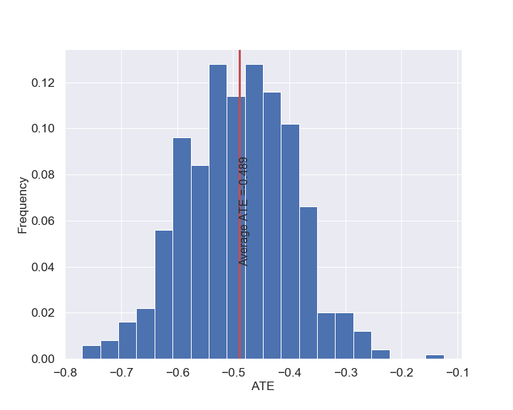
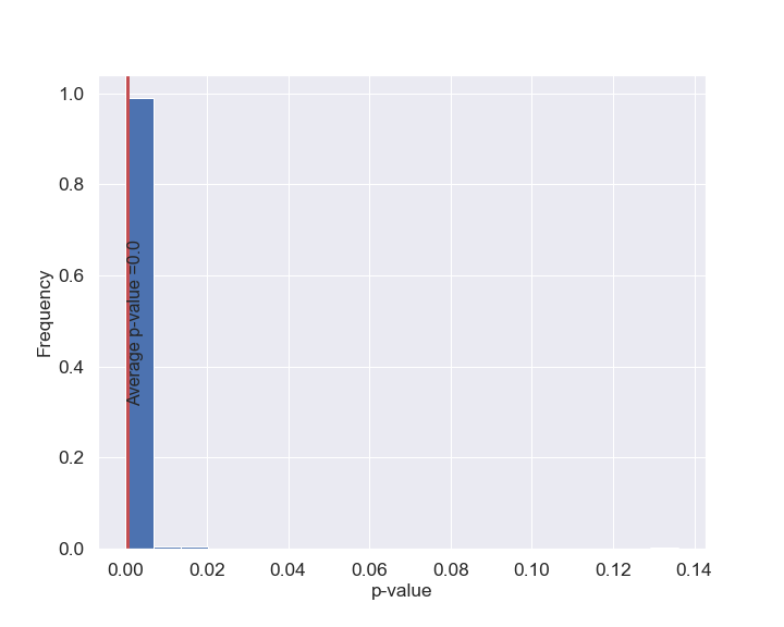
D.2 Mediation analysis for the effect of LCD on CVD

We provide details on assessing the significance of reduction in Reynolds risk score due to the low-carbohydrate using the I-Rand algorithm. The causal diagrams are shown in Figure 6 for the direct and indirect effects. We show the distribution of ATE for the subsampling step in Figure 19 and the distribution of the p-values from the permutation test under the null hypothesis of no causal effect (ATE = 0) in Figure 20, for the total effect (sum of direct and indirect effect); and correspondingly, Figures 21 and 22, for the direct effect. The distributions confirm the consistency of these results across the subsamples.

Figure 19: Distribution of total effect of the LCD on the Reynold risk score in Figure 6. The results are from 500 subsamples.

Figure 20: Distribution of p-values the total effect of the LCD on the Reynolds risk score in Figure 6. The results are based on 500 subsamples.

Figure 21: Distribution of the direct effect of the LCD on the Reynolds risk score in Figure 6. The results are based on 500 subsamples.

Figure 22: Distribution of p-values of the direct effect of the LCD on the Reynold risk score in Figure 6. The results are based on 500 subsamples.

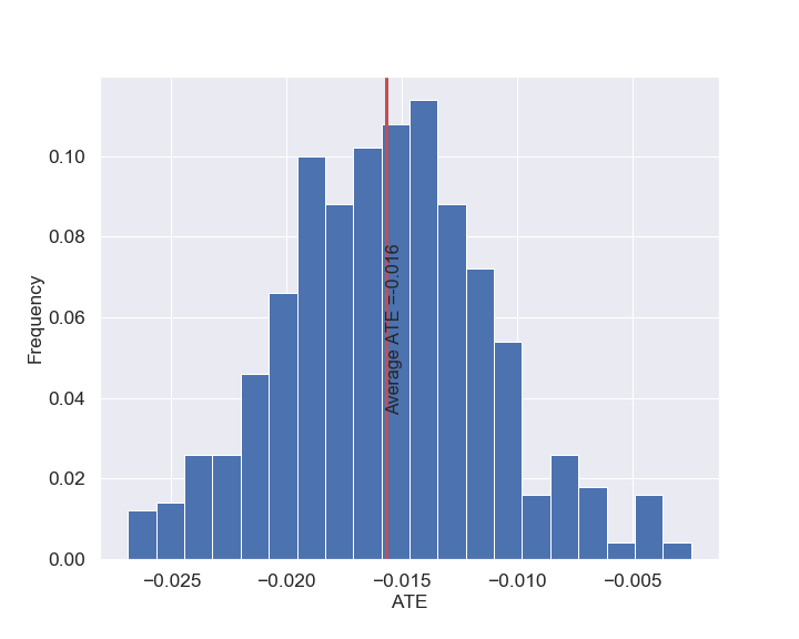
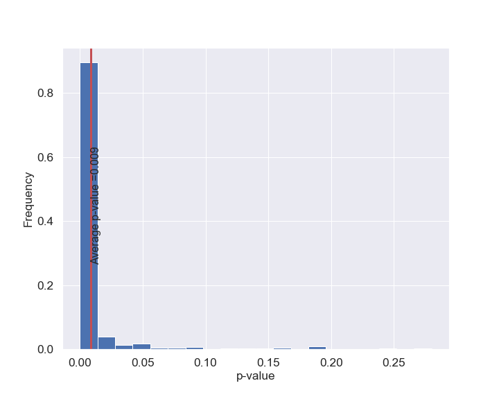
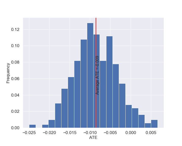
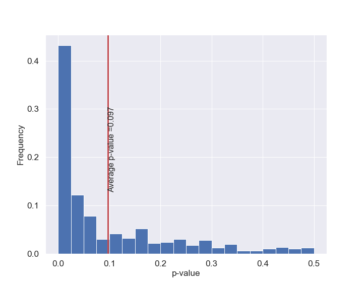
D.3 Causal effect of obesity on T2D

We provide additional details on testing the significance of obesity as a cause of T2D, where the causal diagram is shown in Figure 9. In particular, we show the distribution of ATE for the subsampling step in Figure 23 and the distribution of p-values from the permutation test under the null hypothesis of no causal effect (ATE = 0) in Figure 24, using the I-Rand algorithm. The distributions confirm the consistency of these results across the subsamples.

Figure 23: Distributions of ATE of obesity on T2D in Figure 9. The results are based on 500 subsamples with different BMI splits.

Figure 24: Distributions of p-values of the ATE of obesity on T2D in Figure 9. The results are based on 500 subsamples with different BMI splits.

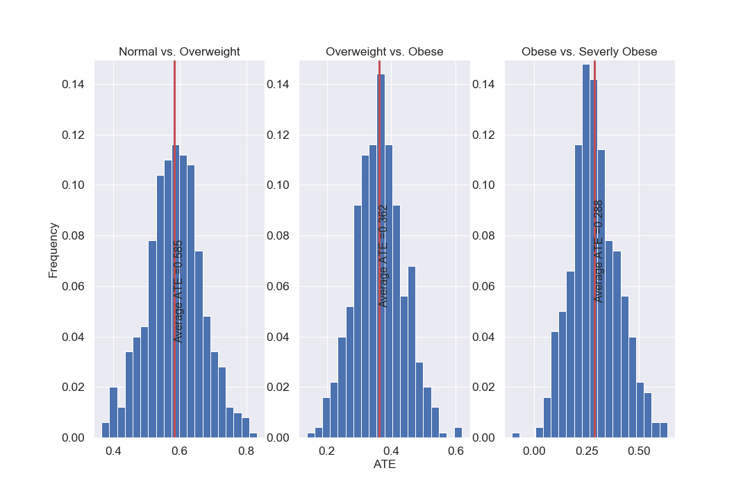
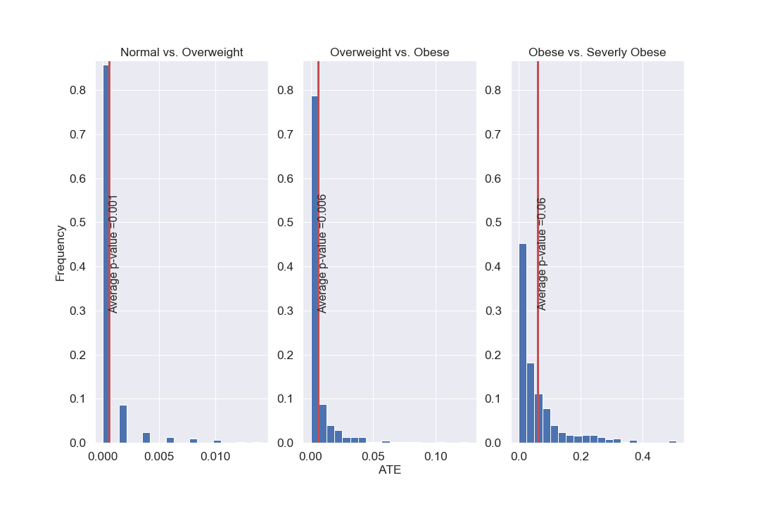
D.4 Mediation analysis for the effect of obesity on CVD

We provide results on testing the significance of. the effect of obesity on high systolic blood pressure, according to the proposed I-Rand algorithm. The causal diagrams are shown in Figure 11 for the direct and indirect effects. In particular, we show the distribution of ATE for the subsampling step in Figure 25 and the distribution of the p-value from the permutation test under the null hypothesis of no causal effect (ATE = 0) in Figure 26, for the total effect; and correspondingly, Figures 27 and 28, for the direct effect. The distributions confirm the causal effect of the obesity to CVD consistently across the subsamples.

Figure 25: Distributions of the total effect of obesity on the systolic blood pressure in Figure 11. The results are based on 500 subsamples with different BMI splits.

Figure 26: Distributions of p-values of the total effect of obesity on the systolic blood pressure in Figure 11. The results are based on 500 subsamples with different BMI splits.

Figure 27: Distributions of the direct effect of obesity on the systolic blood pressure in Figure 11. The results are based on 500 subsamples with different BMI splits.

Figure 28: Distribution of p-values of the direct effect of obesity on the systolic blood pressure in Figure 11. The results are based on 500 subsamples with different BMI splits.

References

- 1 Roth GA, Johnson CO, Abate KH, et al. The burden of cardiovascular diseases among US states, 1990-2016. JAMA Cardiology 2018; 3(5): 375–389.
- 2 Unwin D, Unwin J, Khalid AA, et al. Insights from a general practice service evaluation supporting a lower carbohydrate diet in patients with type 2 diabetes mellitus and prediabets. BMI Nutrition, Prevention and Health (accepted) 2020.
- 3 Morrish NJ, Wang SL, Stevens LK, Fuller JH, Keen H, Group WMS. Mortality and causes of death in the WHO Multinational Study of Vascular Disease in Diabetes. Diabetologia 2001; 44(2): S14.
- 4 Jan S, Laba TL, Essue BM, et al. Action to address the household economic burden of non-communicable diseases. The Lancet 2018; 391(10134): 2047–2058.
- 5 Benjamin EJ, Virani SS, Callaway CW, et al. Heart disease and stroke statistics—2018 update: a report from the American Heart Association. Circulation 2018.
- 6 Scheen AJ, Van Gaal LF. Combating the dual burden: therapeutic targeting of common pathways in obesity and type 2 diabetes. The Lancet Diabetes & Endocrinology 2014; 2(11): 911-922. doi: https://doi.org/10.1016/S2213-8587(14)70004-X
- 7 Bazzano LA, Hu T, Reynolds K, et al. Effects of low-carbohydrate and low-fat diets: a randomized trial. Annals of Internal Medicine 2014; 161(5): 309–318.
- 8 Meng Y, Bai H, Wang S, Li Z, Wang Q, Chen L. Efficacy of low carbohydrate diet for type 2 diabetes mellitus management: a systematic review and meta-analysis of randomized controlled trials. Diabetes Research and Clinical Practice 2017; 131: 124–131.
- 9 Gjuladin-Hellon T, Davies IG, Penson P, Amiri Baghbadorani R. Effects of carbohydrate-restricted diets on low-density lipoprotein cholesterol levels in overweight and obese adults: A systematic review and meta-analysis. Nutrition Reviews 2019; 77(3): 161–180.
- 10 Zuuren vEJ, Fedorowicz Z, Kuijpers T, Pijl H. Effects of low-carbohydrate-compared with low-fat-diet interventions on metabolic control in people with type 2 diabetes: A systematic review including GRADE assessments. The American Journal of Clinical Nutrition 2018; 108(2): 300–331.
- 11 Lean ME, Leslie WS, Barnes AC, et al. Primary care-led weight management for remission of type 2 diabetes (DiRECT): an open-label, cluster-randomised trial. The Lancet 2018; 391(10120): 541–551.
- 12 Vale dMRL, Buckner L, Mitrofan CG, et al. A synthesis of pathways linking diet, metabolic risk and cardiovascular disease: a framework to guide further research and approaches to evidence-based practice. Nutrition Research Reviews 2021: 1–27.
- 13 Hahn U. A studentized permutation test for the comparison of spatial point patterns. Journal of the American Statistical Association 2012; 107(498): 754–764.
- 14 Beck N, Katz JN. What to do (and not to do) with time-series cross-section data. American Political Science Review 1995: 634–647.
- 15 Wilson SE, Butler DM. A lot more to do: The sensitivity of time-series cross-section analyses to simple alternative specifications. Political Analysis 2007: 101–123.
- 16 Angrist JD, Pischke JS. Mostly Harmless Econometrics: An Empiricist’s Companion. Princeton University Press . 2008.
- 17 Bertrand M, Duflo E, Mullainathan S. How much should we trust differences-in-differences estimates?. The Quarterly Journal of Economics 2004; 119(1): 249–275.
- 18 Lavie CJ, Milani RV, Ventura HO. Obesity and cardiovascular disease: risk factor, paradox, and impact of weight loss. Journal of the American College of Cardiology 2009; 53(21): 1925–1932.
- 19 Halton TL, Liu S, Manson JE, Hu FB. Low-carbohydrate-diet score and risk of type 2 diabetes in women. The American Journal of Clinical Nutrition 2008; 87(2): 339–346.
- 20 Koning dL, Fung TT, Liao X, et al. Low-carbohydrate diet scores and risk of type 2 diabetes in men. The American Journal of Clinical Nutrition 2011; 93(4): 844–850.
- 21 Anderson KM, Odell PM, Wilson PW, Kannel WB. Cardiovascular disease risk profiles. American Heart Journal 1991; 121(1): 293–298.
- 22 Ridker PM, Buring JE, Rifai N, Cook NR. Development and validation of improved algorithms for the assessment of global cardiovascular risk in women: the Reynolds Risk Score. JAMA 2007; 297(6): 611–619.
- 23 Neyman J. On the application of probability theory to agricultural experiments. Essay on principles. Section 9. (Trans. Dorota M. Dabrowska and Terence P. Speed.). Statistical Science. 1923 [1990]: 465–472.
- 24 Rubin DB. Estimating causal effects of treatments in randomized and nonrandomized studies.. Journal of Educational Psychology 1974; 66(5): 688.
- 25 Rubin DB, Thomas N. Matching using estimated propensity scores: relating theory to practice. Biometrics 1996: 249–264.
- 26 Imbens GW. Nonparametric estimation of average treatment effects under exogeneity: A review. Review of Economics and Statistics 2004; 86(1): 4–29.
- 27 Rosenbaum PR, Rubin DB. The central role of the propensity score in observational studies for causal effects. Biometrika 1983; 70(1): 41–55.
- 28 Rubin DB. Bias reduction using Mahalanobis-metric matching. Biometrics 1980: 293–298.
- 29 Cox DR. Planning of Experiments. New York: John Wiley & Sons . 1958.
- 30 Neyman J. Statistical problems in agricultural experimentation. Journal of the Royal Statistical Society 1935; 2(2): 107–154.
- 31 Pearl J. Causality. Cambridge University Press . 2009.
- 32 Chernozhukov V, Chetverikov D, Demirer M, et al. Double/debiased machine learning for treatment and structural parameters. The Econometrics Journal 2018: C1–C68.
- 33 Dai X, Li L. Orthogonalized kernel debiased machine learning for multimodal data analysis. Journal of the American Statistical Association 2022: 1–15.
- 34 Abadie A, Gardeazabal J. The Economic Costs of Conflict: A Case Study of the Basque Country.. American Economic Review 2003; 93(1): 112–132.
- 35 Abadie A, Diamond A, Hainmueller J. Synthetic control methods for comparative case studies: Estimating the effect of California’s tobacco control program. Journal of the American statistical Association 2010; 105(490): 493–505.
- 36 McKay MD, Beckman RJ, Conover WJ. A comparison of three methods for selecting values of input variables in the analysis of output from a computer code. Technometrics 2000; 42(1): 55–61.
- 37 Edgington E, Onghena P. Randomization Tests. CRC Press . 2007.
- 38 VanderWeele TJ, Hernan MA. Causal inference under multiple versions of treatment. Journal of Causal Inference 2013; 1(1): 1.
- 39 Zhao Q, Hastie T. Causal interpretations of black-box models. Journal of Business & Economic Statistics 2019; 39.
- 40 Accurso A, Bernstein RK, Dahlqvist A, et al. Dietary carbohydrate restriction in type 2 diabetes mellitus and metabolic syndrome: Time for a critical appraisal. Nutrition & Metabolism 2008; 5(1): 9.
- 41 Martín-Timón I, Sevillano-Collantes C, Segura-Galindo A, Cañizo-Gómez dFJ. Type 2 diabetes and cardiovascular disease: have all risk factors the same strength?. World Journal of Diabetes 2014; 5(4): 444.
- 42 Sowers JR. Obesity as a cardiovascular risk factor. The American Journal of Medicine 2003; 115(8, Supplement 1): 37-41. Evaluating the Cardiovascular Effects of the Thiazolidinediones and Their Place in the Management of Type 2 Diabetes Mellitusdoi: https://doi.org/10.1016/j.amjmed.2003.08.012
- 43 Pearl J. Direct and indirect effects. Proceedings of the Seventeenth Conference onUncertainty in Artificial Intelligence 2001: 411–420.
- 44 Yoon KH, Lee JH, Kim JW, et al. Epidemic obesity and type 2 diabetes in Asia. The Lancet 2006; 368(9548): 1681–1688.
- 45 Bundy JD, Li C, Stuchlik P, et al. Systolic blood pressure reduction and risk of cardiovascular disease and mortality: a systematic review and network meta-analysis. JAMA Cardiology 2017; 2(7): 775–781.
- 46 Uretsky S, Messerli FH, Bangalore S, et al. Obesity paradox in patients with hypertension and coronary artery disease. The American Journal of Medicine 2007; 120(10): 863–870.
- 47 Bareinboim E, Tian J. Recovering causal effects from selection bias. Twenty-Ninth AAAI Conference on Artificial Intelligence 2015.
- 48 Bareinboim E, Pearl J. Causal inference and the data-fusion problem. Proceedings of the National Academy of Sciences 2016; 113(27): 7345–7352.
- 49 Raudenbush SW. Comparing personal trajectories and drawing causal inferences from longitudinal data. Annual Review of Psychology 2001; 52(1): 501–525.
- 50 Heckman JJ, Ichimura H, Todd P. Matching as an econometric evaluation estimator. Review of Economic Studies 1998; 65(2): 261–294.
- 51 Greenland S. Quantifying biases in causal models: classical confounding vs collider-stratification bias. Epidemiology 2003; 14(3): 300–306.
- 52 Dehejia RH, Wahba S. Propensity score-matching methods for nonexperimental causal studies. Review of Economics and Statistics 2002; 84(1): 151–161.
- 53 Rubin DB. Using propensity scores to help design observational studies: application to the tobacco litigation. Health Services and Outcomes Research Methodology 2001; 2(3-4): 169–188.
- 54 Gelber RP, Gaziano JM, Orav EJ, Manson JE, Buring JE, Kurth T. Measures of obesity and cardiovascular risk among men and women. Journal of the American College of Cardiology 2008; 52(8): 605–615.