Low-complexity graph-based traveling wave models for HVDC grids with hybrid transmission lines: Application to fault identification

Abstract

The fast protection of meshed HVDC grids requires the modeling of the transient phenomena affecting the grid after a fault. In the case of hybrid lines comprising both overhead and underground parts, the numerous generated traveling waves may be difficult to describe and evaluate. This paper proposes a representation of the grid as a graph, allowing to take into account any waves traveling through the grid. A relatively compact description of the waves is then derived, based on a combined physical and behavioral modeling approach. The obtained model depends explicitly on the characteristics of the grid as well as on the fault parameters. An application of the model to the identification of the faulty portion of an hybrid line is proposed. The knowledge of the faulty portion is profitable as faults in overhead lines, generally temporary, can lead to the reclosing of the line.

I Introduction

The integration of renewable energy sources leads to the evolution of the existing transmission and distribution power grids into a more interconnected system, known as smart grid [8]. For high voltage transmission, direct current (HVDC) technology may outperform HVAC for long distance interconnections, in particular for underground or undersea cables [1]. In Europe, cables, despite their more important cost, are more and more preferred to overhead lines (OHL) due to the difficulty to obtain new right-of-ways for aerial corridors. It is however possible to upgrade existing HVAC OHL to HVDC, thus increasing the transmission capacity [9]. The recourse to hybrid lines comprising portions of cables and overhead lines permits a better adaption to different terrains and configurations (offshore connection, populated areas, existing corridors etc.), see for instance [14]. Such hybrid lines can be further integrated into larger Multi-Terminal DC grids (MTDC) to increase the overall reliability while decreasing the investment costs.

The protection of MTDC grids against faults remain an open and challenging topic [10]. The selective clearing of faults by disconnecting only the affected line is usually the preferred solution as it allows to operate the healthy parts of the grid continuously. This requires DC Circuit Breakers (DCCB) at the extremity of each line. Each DCCB is then controlled by the neighboring relay which must be able to send the tripping orders as fast as possible (typically in less than 1 ms). The protection algorithm at the relay must thus be able to distinguish faults occurring in the protected line (internal faults) from faults occurring in other parts of the grid (external faults). Furthermore, in the case of hybrid lines, the identification of the faulty segment is of interest. While faults affecting cables are permanent, faults affecting OHL are often temporary and a re-closing of the line may be attempted. The identification of the faulty segment within an hybrid line is a difficult task. Many existing approaches involve distributed sensors at the junction between each portion and synchronized communication between distant sub-stations, as in [12]. On the other hand, single-ended algorithms only require sensors at the extremity of each line and are thus less sensitive to communication issues.

For HVAC lines, [2] proposed a double-ended method using the arrival times at the two extremities of the hybrid line to estimate the fault location. The method shows good localization performance and uncertainty in the line parameters is taken into account to assess the precision of the estimated fault distance.

In [5], a Support Vector Machine (SVM) algorithm is trained to classify the faults of a two segments hybrid line using single ended data. Voltage and current wavelet energies are used as inputs for the SVM. Once the faulty section is identified, a wavelet-based localization technique is applied. As it uses a binary classifier, this approach is limited to hybrid lines with only two segments. The SVM has also to be trained with sufficient fault scenarios. For a Point-to-Point (P2P) hybrid line, [4] showed that the presence of oscillations in the current evolution after the operation of the ACCBs is characteristic of a fault in the overhead part of the line. This kind of approach is not suited for meshed grid where ACCBs do not operate as primary protection.

The presence of sensors at the junction is considered in [11]. A differential protection criterion is then applied to identify the faulty section, assuming the primary protection is ensured through the control of full-bridge Modular Multilevel Converter (MMC). Distributed sensors are also assumed in [12] in the more general case of an hybrid link embedded in a MTDC grid. The primary protection is ensured by a differential current criterion formulated at the junction points. Localization is then performed using the arrival time difference at the different sensors, measured through a wavelet transform of the current.

Model-based approaches representing the transient behavior of the grid are beneficial as they allow one to exploit the information contained in the traveling waves appearing after a fault occurrence, see for instance [13]. In the case of hybrid lines, however, the presence of interconnections along the lines render the evaluation of a large number of traveling waves an arduous task.

This paper proposes a systematic description of the traveling waves appearing after a fault using a a graph description of the grid. For each wave, the proposed model combines a physical and a behavioral part to represent the propagation delays as well as the distortion due to the ground effects, as detailed in Section II. An application example of the model to identify the faulty segment within a hybrid line is presented in Section III. Simulation results using a test grid implemented in EMTP-RV [7] software are presented in Section IV.

In what follows, Laplace domain or frequency domain variables are in capital letters, whereas continuous and discrete time domain variables are in small letters. The convolution is represented by $\otimes$. $\mathcal{F}$ and $\mathcal{F}^{-1}$ stand for the direct and inverse Fourier transform.

II Systematic fault modeling

The section details the modeling of faults affecting hybrid transmission lines embedded in an MTDC grid with monopolar configuration. The main notations are introduced in Section II-A. The TW theory is briefly recalled in Section II-B and the proposed approach for the systematic modeling of TW is presented. The behavioral part of the proposed model to account for the soil resistivity is described in Section II-C.

II-A Overview and notations

The considered network is described as an undirected graph $\mathcal{G}=(\mathcal{Q},\mathcal{E})$. Each vertex $q\in\mathcal{Q}$ represents an interconnection between two or more line segments. Nodes may correspond to bus-bars or junctions between overhead line and underground cable segments. Each segment is represented by an edge $e\in\mathcal{E}$ of the graph. The edge between the nodes $q_{i}$ and $q_{j}$ is denoted $e_{q_{i}q_{j}}$, or $e_{i,j}$ to lighten the notations. Since the graph is undirected, $e_{i,j}=e_{j,i}$. The length of the segment represented by the edge $e_{i,j}$ is $d_{i,j}$.

We assume that at $t=t_{\text{f}}$ a fault occurs in edge $e_{\text{f}}=e_{i,j}\in\mathcal{E}$ and is modeled as a switch closing in series with the fault resistance $R_{\text{f}}$ and a constant voltage source. The voltage source accounts for the collapse of voltage and is set to the opposite of the pre-fault voltage $V_{\text{bf}}$ at the fault location.

The fault leads to a modification of the graph $\mathcal{G}$. A node $q_{\text{f}}$ is added to $\mathcal{Q}$ and the faulty edge $e_{\text{f}}=e_{i,j}\in\mathcal{E}$ is replaced by the edges $e_{i,\text{f}}$ and $e_{\text{f},j}$ of lengths $d_{\text{f},i}$ and $d_{\text{f,}j}$. Formally, the graph $\mathcal{G}_{\text{f}}=\big{(}\mathcal{Q}_{\text{f}},\mathcal{E}_{\text{f}}\big{)}$, once the fault has occurred, is such that $\mathcal{Q}_{\text{f}}=\mathcal{Q}\cup\left\{q_{\text{f}}\right\}$ and $\mathcal{E}_{\text{f}}=\mathcal{E}\textbackslash\{e_{\text{f}}\}\cup\big{\{}e_{i,\text{f}},e_{j,\text{f}}\big{\}}$. The fault can thus be characterized by the vector of fault parameters $\mathbf{p}=\left(t_{\text{f}},e_{\text{f}},d_{\text{f},i},d_{\text{f},j},R_{\text{f}}\right)$, where $R_{\text{f}}$ is the fault resistance between the transmission line and the ground. The two fault distances $d_{\text{f},i}$ and $d_{\text{f},j}$ are linked through the total length of the line $d_{\text{f},i}+d_{\text{f},j}=d_{i,j}$, which is known. Thus only one unknown fault distance is kept, for a fault located on the edge $e_{i,j}$, the fault distance is arbitrarily defined as

$$d_{\text{f}}=\left\{\begin{array}[]{cc}d_{\text{f},i}&\text{ if }i<j\\ d_{\text{f},j}&\text{ if }j<i\end{array}\right..$$ (1)

II-B DC fault physical modeling

This section presents a model describing the transient behavior after the occurrence of a fault. Preliminaries on traveling waves are first recalled in Section II-B1. The proposed systematic modeling approach to describe any wave traveling from the fault through the grid is presented in Section II-B2.

II-B1 Traveling waves

Consider an edge $e_{i,j}$ belonging to a meshed grid such as that presented in Figure 4. The evolution with time of the current and voltage at a given point of $e_{i,j}$ can be described using traveling waves, as shown in [16]. Along the line, current and voltage satisfy the telegraph equations, expressed in the Laplace domain as

$$\frac{\partial^{2}V}{\partial x^{2}} =Z(s)Y(s)V(x,s),$$ (2)

$$\frac{\partial^{2}I}{\partial x^{2}} =Z(s)Y(s)I(x,s),$$ (3)

where $Z(s)=R+sL$ and $Y(s)=G+sC$ are the transfer functions of the distributed series impedance and shunt admittance, respectively. In what follows, the distributed parameters $R,L,C$, and $G$ are considered at a fixed given frequency.

Consider a fault occurring on edge $e_{i,j}$. Two voltage and current waves $V_{i,1}$ and $V_{j,1}$ travel from the fault location along the line towards node $q_{i}$ and $q_{j}$, respectively. They undergo attenuation and distortion described by some propagation function $H$

$$V_{i,1}\left(s,d_{\text{f},i}\right) =H\left(s,d_{\text{f},i}\right)V_{\text{init}}(s)$$ (4)

$$V_{j,1}\left(s,d_{\text{f},j}\right) =H\left(s,d_{\text{f},j}\right)V_{\text{init}}(s),$$ (5)

where $V_{\text{init}}$ is the initial surge at fault location. $H$ can be expressed, for a traveled distance $d$ along the line, as

$$H\left(s,d\right)=\exp\left(-\sqrt{Y(s)Z(s)}d\right).$$ (6)

Any voltage traveling wave $V$ has an associated current wave defined as

$$I(s,d)=Z_{\text{s}}^{-1}(s)V(s,d),$$ (7)

where

$$Z_{\text{s}}\left(s\right)=\sqrt{Z(s)/Y(s)}$$ (8)

is the surge (or characteristic) impedance. Similar computations can be performed for the current.

Getting explicit expressions of the surge impedance and propagation function requires several approximations. Considering a low-loss approximation, one has

$$Z_{\text{s}}\left(s\right)=\sqrt{\frac{R+sL}{G+sC}}\simeq\sqrt{\frac{L}{C}}\left(1+\frac{1}{2}\left(\frac{R}{sL}-\frac{G}{sC}\right)\right).$$

Further neglecting the shunt admittance $G$, one gets

$$Z_{\text{s}}\left(s\right)\simeq\sqrt{\frac{L}{C}}\left(1+\frac{1}{2}\frac{R}{sL}\right).$$ (9)

For the propagation constant $\gamma\left(s\right)=\sqrt{Y(s)Z(s)}$, the low-loss approximation leads to

$$\gamma\left(s\right)\simeq s\sqrt{LC}\left[1+\frac{1}{2}\left(\frac{R}{sL}+\frac{G}{sC}\right)\right]$$

and neglecting again the shunt admittance $G$,

$$\gamma\left(s\right)\simeq s\sqrt{LC}\left[1+\frac{1}{2}\frac{R}{sL}\right].$$ (10)

Considering the lossless approximation, one gets

$$Z_{\text{s}} \simeq\sqrt{\frac{L}{C}}$$ (11)

$$\gamma\left(s\right) \simeq s\sqrt{LC}$$ (12)

In that case, the surge impedance is real and the propagation function $H\left(s,d\right)=\exp\left(-\gamma\left(s\right)d\right)$ is a pure delay.

In practice, the lossless approximations appears to be sufficient in the considered fault localization context. Nevertheless, the characteristic impedance of underground cables still require a low-loss approximation to provide results of sufficient accuracy.

When a change of propagation medium occurs (typically at the junction between a line and a station), the incident wave $V_{\text{f}}$ induces a transmitted wave $V_{\text{t}}$ and a reflected wave $V_{\text{r}}$. The associated voltage $V_{\text{tot}}$ at the junction is

$$V_{\text{tot}} =V_{\text{t}}=V_{\text{f}}+V_{\text{r}}$$

$$=\left(1+K\right)V_{\text{f}}$$

$$=TV_{\text{f}}.$$ (13)

The transmission and reflection coefficients $T$ and $K$ depend on the characteristic admittance $Y_{\text{s}}=Z_{\text{s}}^{-1}$ of the media. Consider a node $q$ connected to $n+1$ edges $e_{0},e_{1},\dots e_{n}$, the reflection coefficient for a wave traveling from edge $e_{0}$, reflected at node $q$, an traveling backwards $e_{0}$ is

$$K_{e_{0}\hookleftarrow q} =\frac{Y_{e_{0}}-\sum_{\ell=1}^{n}Y_{s,e_{\ell}}}{\sum_{\ell=0}^{n}Y_{s,e_{\ell}}}.$$ (14)

The transmission coefficient from edge $e_{0}$ through node $q$, $i=1,\dots,n$ is

$$T_{e_{0}\shortrightarrow q}=1+K_{e_{0}\hookleftarrow q}=\frac{2Y_{s,e_{0}}}{\sum_{\ell=0}^{n}Y_{s,e_{\ell}}}.$$ (15)

Since the fault is modeled as a switch closing at $t=t_{\text{f}}$ in series with the fault resistance $R_{\text{f}}$ and a constant voltage source of amplitude $V_{\text{bf}}$, the initial surge at the fault location $V_{\text{init}}$ is thus modeled as

$$V_{\text{init}} =\underbrace{\frac{-1/R_{\text{f}}}{2/Z_{\text{s}}+1/R_{\text{f}}}}_{K_{e_{i,\text{f}}\hookleftarrow e_{\text{f}}}}V_{\text{bf}}\exp\left(-st_{\text{f}}\right)$$ (16)

which can also be expressed using the reflection coefficient from the line to the fault $K_{e_{i,\text{f}}\hookleftarrow e_{\text{f}}}.$ The voltage at the fault location just before the fault occurrence $V_{\text{bf}}$ can be approximated by the measured pre-fault voltage at the relay $q$.

For reflection and transmission at sub-stations comprising MMCs, we adopt an RLC equivalent model [3], which is valid before the blocking of the station

$$Z_{\text{mmc}}\left(s\right)=R_{\text{mmc}}+sL_{\text{mmc}}+\frac{1}{sC_{\text{mmc}}}.$$ (17)

The propagation equations (4) and (5) combined with the reflection and transmission equations (13), (14), and (15) allow one to model any particular wave traveling from the fault to the grid. Nevertheless, a faulty grid comprising hybrid lines will host many reflected waves due to the multiple junctions. A systematic approach describing these traveling waves is thus required and detailed in Section II-B2.

II-B2 Systematic model of traveling waves within a grid

Consider a node $q_{\text{s}}\in\mathcal{Q}_{\text{f}}$ at which voltage and current are observed. This node may, for instance, connect multiple transmission lines to a converter station. The aim in what follows is to propose a physical model of the TWs caused by the fault and reaching $q_{\text{s}}$. A TW is entirely determined by its path, i.e., the sequence of nodes it has traversed. Formally, all possible paths from $q_{\text{f}}$ to $q_{\text{s}}$ can be defined as

$$\mathcal{P}_{q_{\text{f}}\shortrightarrow q_{\text{s}}}=\left\{\left(q_{n_{1}},..,q_{n_{m}}\right)|\right.\\ \left.q_{n_{1}}=q_{\text{f}},q_{n_{m}}=q_{\text{s}},\left(q_{n_{i}},q_{n_{i+1}}\right)\in\mathcal{E}_{\text{f}},m>1\right\}$$ (18)

A path $\pi\in\mathcal{P}_{q_{\text{f}}\shortrightarrow q_{\text{s}}}$ may comprise the same node several times, including the faulty node $q_{\text{f}}$ and the observation node $q_{\text{s}}$. Due to the reflections occurring at the junctions, a TW is indeed likely to pass several times via the same nodes. Considering the lossless approximation and constant distributed parameters, as in Section II-B1 when a wave travels on an edge, only the propagation delay has to be taken into account. Consequently, when modeling traveling waves, one has to account for

• the different delays due to the propagation along the edges,

• the effect of junctions on the incident wave.

Consider a path $\pi=\left(q_{n_{1}},..,q_{n_{m}}\right)\in\mathcal{P}_{q_{\text{f}}\shortrightarrow q_{\text{s}}}$ traveled by a given wave. The total propagation delay along $\pi$ is

$$\tau_{\pi}(d_{\text{f}})=\sum_{i=1}^{m}\Delta t_{n_{i},n_{i+1}}=\sum_{i=1}^{m-1}\frac{d_{n_{i},n_{i+1}}}{c_{n_{i},n_{i+1}}}$$ (19)

where $c_{n_{i},n_{i+1}}$ is the wave propagation speed along the edge $\left(q_{n_{i}},q_{n_{i+1}}\right)$, depending on the propagation medium. The total delay thus depends on the fault distances $d_{\text{f},i}$ or $d_{\text{f,}j}$ as at least the first traversed edge is necessarily connected to the fault.

At each junction along $\pi$, the voltage wave is subject to a transmission and a reflection. The resulting coefficient depends on the propagation direction before and after the junction. Consequently, the impact of reflections and transmissions at junctions is described by

$$V_{\pi,\text{j}}(s,t_{\text{f}},R_{\text{f}})=\prod_{i=1}^{m}J_{e_{n_{i-1},n_{i}}\shortrightarrow q_{n_{i}}}(s,R_{\text{f}})\frac{\exp(-t_{\text{f}}s)}{s}V_{\text{bf}}$$ (20)

where $J$ is either a reflection (14) or transmission (15) coefficient

$$J_{e_{n_{i-1},n_{i}}\shortrightarrow q_{n_{i}}}=\left\{\begin{array}[]{cc}T_{e_{n_{i-1},n_{i}}\shortrightarrow q_{n_{i}}}&\text{ if }n_{i-1}\neq n_{i+1}\\ K_{e_{n_{i-1},n_{i}}\hookleftarrow q_{n_{i}}}&\text{ if }n_{i-1}=n_{i+1}\end{array}\right.$$

for $i=2,\dots,m-1$. The first term in the product (20) accounts for the initial surge at the fault location $J_{e_{n_{0},n_{i}}\shortrightarrow q_{n_{1}}}=K_{q_{{}_{n_{1}},},q_{{}_{n_{2}},}\hookleftarrow q_{\text{f}}}\left(R_{\text{f}}\right)$ and depends thus on the fault resistance, see (16). The voltage at node $q_{\text{s}}$ due to the arrival of an incident wave corresponds to the transmitted wave to the node $q_{\text{s}}$ (13). This transmission coefficient is thus included as the last term in the product (20), hence $J_{e_{n_{m-1},n_{m}}\shortrightarrow q_{m}}=T_{e_{n_{m-1},n_{m}}\shortrightarrow q_{\text{s}}}$. Consequently, for a given path $\pi$, considering the propagation delay (19) and the transmissions and reflections occurring along $\pi$ via (20), one gets the following physical model

$$V_{\pi}^{0}\left(s,\mathbf{p}\right)=\exp\left(-\tau_{\pi}(d_{\text{f}})s\right)V_{\pi,\text{j}}(s,t_{\text{f}}R_{\text{f}})$$ (21)

of the voltage caused by a TW along $\pi$.

The different paths taken by the TW can be represented via a Bewley lattice diagram. Figure 1 illustrates such diagram on a point-to-point link consisting of an OHL and a cable segment. Even in this relatively simple case, the presence of the OHL-cable junction creates a large number of reflected TWs. The propagation speed of the TWs in the underground part is slower than in the overhead line.

The waveform in the time domain is obtained through the inverse Fourier transform.

$$v_{\pi}^{0}(t,\mathbf{p}) =\mathcal{F}^{-1}\left\{\left.V_{\pi}^{0}(s,\mathbf{p})\right|_{s=j\omega}\right\}$$

$$=\mathcal{F}^{-1}\left\{V_{\pi,\text{j}}(\omega,R_{\text{f}})\right\}\otimes\delta_{\tau_{\pi}\left(d_{\text{f}}\right)}\left(t\right)$$

$$=v_{\pi,\text{j}}(t,R_{\text{f}})\otimes\delta_{\tau_{\pi}}\left(d_{\text{f}},t\right)$$

$$=v_{\pi,\text{j}}(t-\tau_{\pi}\left(d_{\text{f}}\right),R_{\text{f}})$$ (22)

where $\delta_{\tau_{\pi}\left(d_{\text{f}}\right)}\left(t\right)=\delta_{0}\left(t-\tau_{\pi}\left(d_{\text{f}}\right)\right)$ is the Dirac distribution corresponding to the propagation delay $\tau_{\pi}$ along the path. In practice, $\mathcal{F}^{-1}$ is computed numerically using the inverse discrete Fourier transform. Considering a sampling period $T_{\text{s}}$, the obtained discrete-time voltage model at time $kT_{\text{s}}$ is thus written as $v_{\pi}^{0}\left(k,\mathbf{p}\right)$.

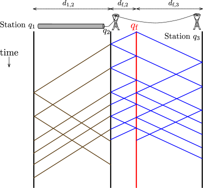
Figure 1: Example of Bewley lattice diagram for a hybrid point-to-point link when a fault occurs as $q_{\text{f}}$ located in an overhead portion of the line.

II-C Behavioral modeling of the ground effects

The physical model developed in Sections II-B1 and II-B2 assumes the distributed line parameters as independent of the frequency. With this approximation, distortions of the waves cannot be described. In particular, the soil resistivity effects for the OHL portions as well as the screen resistance for the cable portions are not taken into account.

To account for such effects, a behavioral model is proposed in this section. It extends to hybrid lines a model previously introduced for overhead lines in [13]. From the geometry of the transmission lines and the characteristics of the conductors, the response for a voltage step propagating along a given edge $e$ can be obtained using EMT simulation software. In particular, the step response depends on the length of the considered segment $d_{e}$ and on the value of the soil resistivity $\rho_{e}$. The latter is considered as a known constant characteristic of the considered line. The propagation delay is removed from the step responses as it is already accounted for by the propagation constant (12).

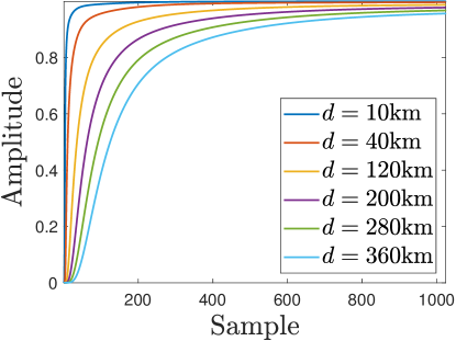
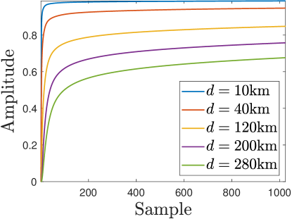
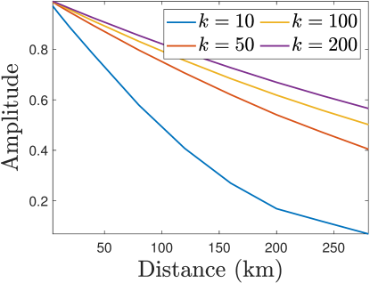
Figure 2: Unit step response for overhead lines (top-left) and cables (bottom-left) of different lengths; The variation of amplitude with the distance for specific sample points is detailed for OHL (top-right) and cables (bottom-right); The sampling frequency is $f_{\text{s}}=1\,\text{MHz}$.

Assume that a set of known step responses $u_{d,\rho}(k)$ for various edge lengths $\left\{d_{1},d_{2},\dots d_{n}\right\}$ is available for a given conductor and line geometry, as presented in Figure 2. The different step responses have smooth variations with respect to the line length. Thus, to obtain a step response $u_{d}$ for any length $d$ such that $d_{i}<d<d_{i+1}$, $i=1,\dots,n-1$ , we propose an interpolation using the step responses obtained for fault distances $d_{i}$ and $d_{i+1}$

$$u_{d}(k)=\frac{u_{d_{i+1}}(k)-u_{d_{i}}(k)}{(d_{i+1}-d_{i})}(d-d_{i})+u_{d_{i}}(k).$$ (23)

The step response of a given edge $e$ is differentiated to obtain the impulse response $h_{e}$

$$h_{e}(k)=\frac{u_{d,\rho}(k+1)-u_{d,\rho}\left(k\right)}{T_{\text{s}}}.$$ (24)

If the step response for the soil resistivity $\rho_{e}$ of the edge $e$ is unknown, it can be interpolated from the step responses at known soil resistivities $\rho_{1},\dots,\rho_{m}$ similarly to (23).

The evolution of a wave traveling through an edge $e$ of length $d_{e}$ is obtained as the output of the finite impulse response filter excited by the output of the physical model (21) of the edge $e$

$$v_{e}^{\text{m}}\text{$\left(k,\mathbf{p}\right)$}=h_{e}\left(k,d_{e}\right)\otimes v_{e}^{0}\left(k,\mathbf{p}\right).$$ (25)

For a wave traveling through a path $\pi\in\mathcal{P}$ comprising several edges, the total voltage evolution at node $q_{\text{s}}$ is obtained by cascading the impulse responses of the different edges, see for example Figure 3

$$v_{\pi}^{\text{m}} \left(k,\mathbf{p}\right)=\underbrace{\bigotimes_{e\in\pi}h_{e}\left(k,d_{e}\right)}_{=h_{\pi}\left(k,d_{\text{f}}\right)}\otimes v_{\pi}^{0}(k,\mathbf{p})$$ (26)

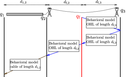
Figure 3: Example of cascaded behavioral model to take into account segmented transmission lines

The global model of the voltage at the node of interest $q_{\text{s}}$ has thus to gather all possible traveling waves between the faulty node $q_{\text{f}}$ and $q_{\text{s}}$

$$v_{q_{\text{s}}}^{\text{m}}\left(\mathbf{p},k\right)=\sum_{\pi\in\mathcal{P}_{q_{\text{f}}\shortrightarrow q_{\text{s}}}}v_{\pi}^{\text{m}}\left(\mathbf{p},k\right).$$ (27)

When considering a finite observation window of duration $\tau_{\text{max}}$ after the occurrence of a fault, only a finite number of traveling waves may reach the node $q_{\text{s}}$ within this time observation window. This reduces the set of paths to consider for simulation

$$\mathcal{P}_{q_{\text{f}}\shortrightarrow q_{\text{s}},\tau_{\text{max}}}=\left\{\pi\in\mathcal{P}_{q_{\text{f}}\shortrightarrow q_{\text{s}}}|\tau_{\pi}<\tau_{\text{max}}\right\}.$$ (28)

An alternative approach to limit the computational complexity is to simulate a maximum number $n_{\text{max}}$ of TWs and to consider as many paths.

III Faulty segment identification

This section describes an extension of the fault identification algorithm presented in [13] in the case of overhead lines only. The estimation of the fault parameters is first summarized in Section III-A. For hybrid lines, the fault identification algorithm must determine whether the line under protection is faulty and assert which of the segments is affected by the fault. Thus leads to a multiple hypothesisis approach, as presented in Section III-B.

III-A Fault parameter estimation

Consider a relay at some node $q$ monitoring a line $L$ described by $m$ edges $\left(e_{1,2},\dots,e_{m-1,m}\right)$ of lengths $\left(d_{1,2},\dots,d_{i,i+1},\dots,d_{m-1,m}\right)$. A fault occurs at time $t_{\text{f}}$ in an edge $e_{\text{f}}=e_{i,i+1}$ within line $L$. The vector of the fault parameters to be estimated is $\mathbf{p}=\left(t_{\text{f}},d_{\text{f}},R_{\text{f}},e_{\text{f}}\right)$. The time at which the first wave induced by the fault reaches node $q$ is related to $t_{\text{f}}$ as

$$t_{\text{d},q}=t_{\text{f}}+\sum_{k=1}^{i-1}\frac{d_{k}}{c_{k}}+\frac{d_{\text{f}}}{c_{i,i+1}}.$$ (29)

We assume that the detection time $t_{\text{d},q}=k{}_{\text{d},q}T_{\text{s}}$ can be accurately measured at the station $q$.

The parametric model developed in Section II is employed to estimate the fault parameters. As, this model requires the faulty edge to be fixed, several hypotheses related to the faulty edge $e_{\text{\text{f}}}$ have to be considered in parallel to estimate the fault parameters $\mathbf{p}=\left(d_{\text{f}},R_{\text{f}},e_{\text{f}}\right)$, where $t_{\text{f}}$ is deduced from $t_{\text{d},q}$ and $d_{\text{f}}$ using (29). Under hypothesis $\mathcal{H}_{\ell}$, the fault is assumed to be located in the edge $e_{\ell,\ell+1}\in\mathcal{E_{\text{f}}}$, $\ell=1,\dots,m-1$ and the vector of parameters to be estimated boils down to $\mathbf{p}_{\ell}=\left(d_{\ell,\text{f}},R_{\text{f}}\right)$.

The algorithm evaluates a maximum likelihood estimate $\mathbf{\widehat{p}}_{\ell}$ of the vector of fault parameters $\mathbf{p}_{\ell}$ using the voltage and current measurements $\left(v_{q}\left(k\right),i_{q}\left(k\right)\right)$ and the model $\left(v_{q,\ell}^{\text{m}}\left(\mathbf{p},k\right),i_{q,\ell}^{\text{m}}\left(\mathbf{p},k\right)\right)$ associated to the hypothesis $\mathcal{H}_{\ell}$. Considering that the voltage and current measurement noises are realizations of independent and identically distributed zero-mean Gaussian variables of respective variances $\sigma_{v}^{2}$ and $\sigma_{i}^{2}$, when $n$ measurements are available, evaluating $\mathbf{\widehat{p}}_{\ell}$ amounts to minimizing the following cost function [15]

$$c_{\ell}^{\left(n\right)}\left(\mathbf{p}\right)=\frac{1}{\sigma_{v}^{2}}\sum_{k=k_{\text{d},q}}^{k_{\text{d},q}+n-1}\left(v_{q,\ell}^{\text{m}}\left(\mathbf{p},k\right)-v_{q}\left(k\right)\right)^{2}+\\ \frac{1}{\sigma_{i}^{2}}\sum_{k=k_{\text{d},q}}^{k_{\text{d},q}+n-1}\left(i_{q,\ell}^{\text{m}}\left(\mathbf{p},k\right)-i_{q}\left(k\right)\right)^{2}.$$ (30)

The algorithm evaluates iteratively an estimate $\mathbf{\widehat{p}}_{\ell}$ of the fault parameters. The estimation algorithm starts when an abnormal behavior is detected at the relay and the estimate

$$\mathbf{\widehat{p}}_{\ell}^{\left(n\right)}=\arg\min_{\mathbf{p}}c_{\ell}^{\left(n\right)}\left(\mathbf{p}\right)$$

is updated when $\Delta n$ new measurements are available. This minimization is performed considering Levenberg-Marquadt’s algorithm, which requires an evaluation of the partial derivatives of $c_{\ell}^{\left(n\right)}\left(\mathbf{p}\right)$ with respect to $d_{\text{f}}$ and $R_{\text{f}}$. This may be done by finite differences, leading to a computational cost which is twice that of evaluating the cost. Appendices -A and -B detail an explicit evaluation of these partial derivatives. Several simplifications are possible, which reduces the complexity of the computations.

III-B Fault identification

For a given hypothesis $\mathcal{H}_{\ell}$, the algorithm determines after each iteration whether $\mathbf{\widehat{p}}_{\ell}^{\left(n\right)}$ is a satisfying estimate of the fault parameters, i.e., if it is compliant with $\mathcal{H}_{\ell}$ regarding the geometry of the edge and if the estimate has been obtained with a sufficient level of confidence. Two tests are employed to confirm or reject the hypothesis $\mathcal{H}_{\ell}$ that the segment $e_{\ell}$ is faulty.

First, a validity test determines whether or not $\mathbf{\widehat{p}}_{\ell}^{\left(n\right)}$ is included in some domain of interest. For instance, the estimated fault distance should be less than the total length of the assumed faulty edge $e_{\ell,\ell+1}$. This domain of interest thus depends on the assumed faulty edge as well as the type of segment, as for instance fault resistances in cables are much lower than in overhead lines.

Second, an accuracy test determines whether the area of the $\alpha$ confidence region of the estimated parameters, $\mathcal{R}^{(\alpha)}(\mathbf{\widehat{p}}_{\ell}^{\left(n\right)})$, is less than a threshold $t_{\alpha}$. The $\alpha=95\%$ confidence region is considered. The confidence region is computed based on the Fisher information matrix, assuming usual statistical properties such as normal independent distribution of the measurement noises, [15]. If both tests are satisfied, the fault is deemed to potentially affect edge $e_{\ell,\ell+1}$. Otherwise, the algorithm waits until $\Delta n$ additional measurements are available to update $\mathbf{\widehat{p}}_{\ell}^{\left(n\right)}$ and $\mathcal{R}^{(\alpha)}(\mathbf{\widehat{p}}_{\ell}^{\left(n\right)})$. Once enough measurements have been made available without allowing to conclude, the hypothesis $\mathcal{H}_{\ell}$ is rejected.

After considering $n$ measurements, several edges $e_{\ell,\ell+1}$ may be deemed to be affected by a fault. Assuming there is a single fault, the algorithm determines which segment is actually faulty by considering the hypothesis with the smallest cost (30)

$$\widehat{e}_{\text{f}}=\arg\min_{e_{\ell,\ell+1}}\left\{c^{\left(n\right)}(\mathbf{p},e_{\ell,\ell+1})|\text{fault is identified on }e_{\ell,\ell+1}\right\}.$$

IV Simulation results

This section presents the results of the fault identification algorithm implementing the hybrid model considering the EMT software EMTP-RV [6] to simulate the behavior of a grid affected by a fault. The test grid is described in Section IV-A. The model proposed in Section II is implemented in Matlab and compared against EMT simulations in Section IV-B. An illustrative example of the fault identification approach is detailed in Section IV-C.

IV-A Test grid

The considered test grid is a four station meshed grid, represented in Figure 4, implemented in the EMT software. Lines $e_{1,2}$ and $e_{1,3}$ are overhead lines. Lines $e_{1,4}$ and $e_{2,4}$ are hybrid lines comprising sections of underground cables and overhead lines. Each transmission line is protected by two relays located at its extremities. The EMT simulations are performed at a sampling frequency $f_{\text{s}}=1\,\text{MHz}$ which also corresponds to the frequency of the measurements.

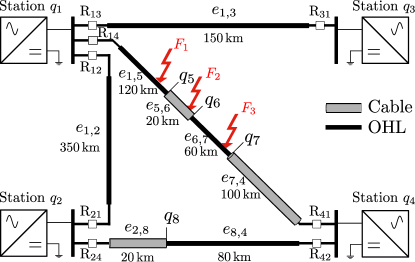
Figure 4: Meshed grid of four converter stations considered for the simulation tests.

The MMC stations are simulated with parameters from Table I and the corresponding equivalent RLC approximation used in the parametric model is given in Table IV. The underground cable and overhead line characteristics are displayed in Tables II and III respectively. The corresponding distributed parameters employed in the parametric model are in Table V.

TABLE I: Characteristics of the MMC stations used for the EMT simulations

Rated power (MVA)	1000
DC rated voltage (kV)	320
Arm inductance (p.u.)	0.15
Capacitor energy in each submodule (kJ/MVA)	40
Conduction losses of each IGBT/diode ($\Omega$)	0.001
Number of sub-modules per arm	400

TABLE II: Underground cable characteristics for the EMT simulations

	Core	Screen
Vertical distance (m)	1.33
Outer radius (mm)	63.9
Inside radius (mm)	0	56.9
Outside radius (mm)	32	58.2
Resistivity (n$\Omega$m)	17.2	28.3

TABLE III: Overhead-line characteristics for the EMT simulations

DC resistance (m$\Omega$/km)	24
Outside diameter (cm)	4.775
Horizontal distance (m)	5
Vertical height at tower (m)	30
Vertical height at mid-span (m)	10
Soil resistivity ($\Omega$m)	100

TABLE IV: Equivalent parameters of the MMC stations used in the parametric model

Equivalent inductance (mH)	8.1
Equivalent resistance ($\Omega$)	0.4
Equivalent capacitance ($\mu$F)	391

TABLE V: Transmission line distributed parameters at $1\,\text{kHz}$ used in the parametric model

	Underground cable	Overhead lines
Series resistance $R$ (m$\Omega$/km)	102	872
Series inductance $L$ (mH/km)	0.123	1.84
Shunt capacitance $C$ (nF/km)	241	7.68
Shunt conductance $G$ (nS/km)	-0.4	0.2

IV-B Modeling results

This section presents the modeling results of the approach proposed in Section II and compares them with EMT simulations. Faults in an underground cable section as well as in an aerial part are both investigated.

IV-B1 Fault in an overhead line section

Consider the fault $F_{1}$ in Figure 4 affecting the line between stations $q_{1}$ and $q_{4}$, on the edge $e_{1,5}$ corresponding to an overhead line section. The fault is located at a distance $d_{\text{f}}=100\,\text{km}$ from the station $q_{1}$ and has an impedance $R_{\text{f}}=5\,\Omega$. The model of the evolution of the voltage and current at the relay $R_{14}$ monitoring this line, located at station $q_{1}$ is compared with the EMT data in Figure 6. The proposed model presents a very good accuracy compared to the EMT simulations for both the current and voltage. The norm of the error in voltage and current are less than 3 kV and 40 A respectively for the considered observation window.

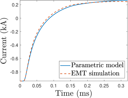
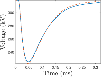
Figure 5: Current and voltage simulation for overhead line fault occurring at $d_{\text{f}}=100\,\text{km}$ from the station $q_{1}$, with a resistance of $R_{\text{f}}=5\,\Omega$, as seen from relay $R_{14}$.

IV-B2 Fault in underground cable section

Consider the fault $F_{2}$ in Figure 4 affecting the line between stations $q_{1}$ and $q_{4}$, on the edge $e_{5,6}$ corresponding to an underground section. The fault is located at a distance $d_{\text{f}}=15\,\text{km}$ from the junction $q_{5}$ and has an impedance of $R_{\text{f}}=0.1\,\Omega$. The obtained model of the evolution of the voltage and current at the relays $R_{14}$ and $R_{41}$ monitoring this line is compared with the EMT simulation result in Figure 6. The norm of the error in voltage and current are less than 6 kV and 50 A respectively for the considered observation window. The fault located $15\,\text{km}$ away from $q_{5}$ and $5\,\text{km}$ from $q_{6}$ results in 3 significant TWs that must be taken into account in the model (the small fault resistance makes the waves reflected at the junction $q_{6}$ negligible).

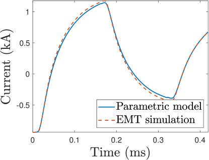
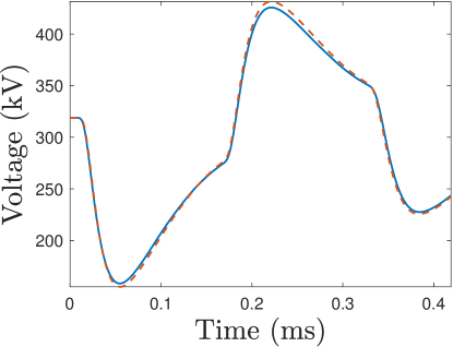
Figure 6: Current (left) and voltage (right) simulation for cable fault occurring at $d_{\text{f}}=135\,\text{km}$ from station 1, with resistance of $R_{\text{f}}=0.1\,\Omega$, as seen from relay $R_{14}$.

The model proposed in Section II is thus able to accurately represent the current and voltage TWs for both underground and overhead line faults.

IV-C Fault localization example

Consider the fault $F_{3}$ in Figure 4 affecting the line between stations $q_{1}$ and $q_{4}$, on the edge $e_{6,7}$ corresponding to an overhead section. The fault is located at $d_{\text{f}}=50\,\text{km}$ from the node $q_{6}$ and has an impedance of $R_{\text{f}}=70\,\Omega$. The behavior of the fault identification approach at the relay $R_{14}$ is analyzed. In the least-squares criterion (30) the voltage and current variances are set such that $\frac{\sigma_{i}^{2}}{\sigma_{v}^{2}}=4$.

Four algorithms are launched in parallel, each corresponding to a different hypothesis relative to the faulty segment. Each algorithm performs similarly: one iteration is performed in the minimization of the cost function (30) every $\Delta n=10$ available new measurements.

The area of the 95% confidence region for the estimated parameters for the four different hypotheses are plotted in Figure 7 (left) and compared with the predetermined threshold $t_{95}=10$. Three different hypotheses satisfy the accuracy test as the area of their confidence region goes below the threshold. Nevertheless, the validity test is not satisfied for the hypothesizes corresponding to the faulty edges $e_{5,6}$ and $e_{7,8}$, as their estimated fault resistances are above $R_{\text{max}}=5\,\Omega$ for the cables, see Figure 7 (right). Considering the assumption that $e_{6,7}$ is the faulty edge, the estimated fault parameters satisfy the validity test as the estimated resistance stays below the maximum fault resistance $R_{\text{max}}=200\,\Omega$ for an overhead section fault.

Thus, the fault is correctly identified after 16 iterations on the edge $e_{6,7}$ when the area of the confidence region for this hypothesis goes below the threshold, see Section III-B. The estimated fault parameters after considering a measurement window of $160\,\mu s$ are $\widehat{R}_{\text{f}}=47\,\Omega,\ \widehat{d}_{\text{f}}=54\,\text{km}$.

In this case, the localization of the fault in an overhead segment indicates it is probably non-permanent and a reclosing of the line may be attempted after some time.

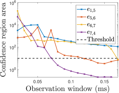
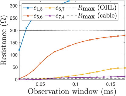
Figure 7: Evolution of the area of the 95% confidence ellipse (left) and value of the estimated fault resistance (right) for each hypothesis.

Figure 8 represents the evolution with the number of iterations of the estimated fault distance and resistance considering the hypothesis of a fault in the (actual faulty) edge $e_{6,7}$.

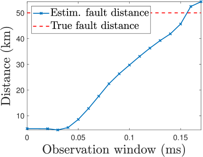
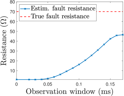
Figure 8: Evolution with time of the estimated fault distance (left) and resistance (right) considering the hypothesis of a fault in the edge $e_{6,7}$ (actual faulty edge).

The waveform of the voltage and current for the EMT simulation and parametric model with the estimated fault parameters are compared in Figure 9. The difference between the model and the EMT data is always less than 10 A for the current and 1 kV for the voltage and is mostly related to the difference between the estimated and actual fault resistance.

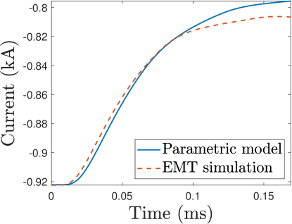
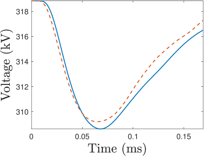
Figure 9: Comparison of the modeled and simulated voltage (right) and current (left) at the relay $R_{14}$. The fault parameters used in the parametric model are the ones obtained after 16 iterations: $\widehat{R}_{\text{f}}=47\,\Omega$ and $\widehat{d}_{\text{f}}=54\,\text{km}$.

V Conclusion

This paper addresses the problem of traveling wave modeling in mixed HVDC lines consisting of both overhead and underground parts. Though EMT tools give an accurate representation of the transient phenomenon occurring in case of a fault, they are ill-suited for protection applications that require the fast evaluation of the transients. A model that describes the transient behavior of the grid is proposed for single conductor overhead lines and underground cables. A representation of the grid and its components as a graph is considered. This allows one to formally describe the multiple traveling waves generated after the fault occurrence due to the reflections and transmissions occurring at each junction within the grid. The obtained model depends explicitly on the grid parameters as well as on the parameters of the fault such as the fault distance and resistance.
When a fault is suspected, the model can be employed for the identification and localization of the faulty segment of the line based on the estimation of the fault parameters. The reclosing of the faulty line can then be attempted if the line affects an overhead line where faults are generally temporary.

In this section the computation of the partial derivatives of the voltage with respect to the fault distance and fault resistance are established in a general case. The obtained expressions can be employed in place of a finite difference approach for gradient evaluations to reduce the computational burden of the parameter estimation algorithm introduced in Section III-A.

A fault is assumed to occur on an edge $e_{\text{f}}$ between nodes $q_{k}$ and $q_{\ell}$ within a grid. The two edges connected to the fault node $q_{\text{f}}$ are denoted as $e_{\text{f},k}$ and $e_{\text{f},\ell}$ and are of lengths $d_{\text{f},k}$ and $d_{\text{f},\ell}$, respectively. Assuming, without loss of generality, that $k<\ell$, according to the fault distance convention 1: $d_{\text{f}}=d_{\text{f},k}$. The computations are detailed for a wave traveling though a path $\pi=\left(q_{n_{1}},\dots,q_{n_{m}}\right)$ where $q_{n_{i}}\in\mathcal{Q}_{\text{f}},\ i=1,\dots,m$ and $q_{n_{1}}=q_{\text{f}}$.

-A Partial derivative with respect to the fault distance

According to (22) and (26), the model of the voltage observed at node $q_{n_{m}}$ resulting from a wave that traveled through the path $\pi$ can be expressed in the times domain as

$$v_{\pi}^{\text{m}}\left(\mathbf{p},k\right)=v_{\pi,\text{j}}\left(R_{\text{f}},\left(k-f_{\text{s}}\tau\left(d_{\text{f}}\right)\right)\right)\varotimes h_{\pi}\left(d_{\text{f}},k\right),$$

where $\tau$ corresponds to the total propagation time through the path $\pi$. The delay $\tau$ only depends on the fault distance $d_{\text{f}}$.

The derivative with respect to the fault distance $d_{\text{f}}$ is then given by (31).

$$\frac{\partial v_{\pi}^{\text{m}}\left(\mathbf{p},k\right)}{\partial d_{\text{f}}} =v_{\pi,\text{j}}\left(R_{\text{f}},k-f_{\text{s}}\tau\left(d_{\text{f}}\right)\right)\varotimes\frac{\partial\left[h_{\pi}\left(d_{\text{f}},k\right)\right]}{\partial d_{\text{f}}}$$ (31)

$$+h_{\pi}\left(d_{\text{f}},k\right)\varotimes\frac{\partial\left[v_{\pi,\text{j}}^{\text{}}\left(R_{\text{f}},k-f_{\text{s}}\tau\left(d_{\text{f}}\right)\right)\right]}{\partial d_{\text{f}}}$$

$$=v_{\pi,\text{j}}^{\text{}}\left(R_{\text{f}},k-f_{\text{s}}\tau\left(d_{\text{f}}\right)\right)\varotimes\frac{\partial\left[h_{\pi}\left(d_{\text{f}},k\right)\right]}{\partial d_{\text{f}}}$$

$$-h_{\pi}\left(d_{\text{f}},k\right)\varotimes f_{\text{s}}\frac{\partial\tau}{\partial d_{\text{f}}}\frac{\partial\left[v_{\pi,\text{j}}^{\text{}}\left(R_{\text{f}},k-f_{\text{s}}\tau\left(d_{\text{f}}\right)\right)\right]}{\partial\left(k-f_{\text{s}}\tau\left(d_{\text{f}}\right)\right)}.$$

The delay $\tau$ due to the propagation along the path $\pi$ can be expended as

$$\tau\left(d_{\text{f}}\right)=\!\sum_{\begin{subarray}{c}i\\ q_{n_{i}}\neq q_{\text{f}}\\ q_{n_{i+1}}\neq q_{\text{f}}\end{subarray}}\tau_{e_{n_{i},n_{i+1}}}+\sum_{\begin{subarray}{c}\begin{subarray}{c}i\\ e_{n_{i},n_{i+1}}=e_{\text{f},k}\end{subarray}\end{subarray}}\tau_{e_{n_{i},n_{i+1}}}+\sum_{\begin{subarray}{c}\begin{subarray}{c}\begin{subarray}{c}i\\ e_{n_{i},n_{i+1}}=e_{\text{f},\ell}\end{subarray}\end{subarray}\end{subarray}}\tau_{e_{n_{i},n_{i+1}}},$$ (32)

where we have isolated the delays due to propagation along the edges $e_{\text{f},k}$ and $e_{\text{f},\ell}$. Introducing $m_{\text{f},k}$ and $m_{\text{f},\ell}$ as the number of times the wave traveled through the two edges connected to the fault $e_{\text{f},k}$ and $e_{\text{f},\ell}$, one gets

$$\tau\left(d_{\text{f}}\right)=\sum_{\begin{subarray}{c}i\\ q_{n_{i}}\neq q_{\text{f}}\\ q_{n_{i+1}}\neq q_{\text{f}}\end{subarray}}\tau_{e_{n_{i},n_{i+1}}}+m_{\text{f},k}\frac{d_{\text{f}}}{c_{e_{\text{f}}}}+m_{\text{f},\ell}\frac{d_{e_{\text{f}}}-d_{\text{f}}}{c_{e_{\text{f}}}}$$

The first sum correspond to propagation times along edges not connected to the faulty node. Hence, assuming the propagation speed does not depend on the fault distance

$$\frac{\partial\tau}{\partial d_{\text{f}}}=\frac{m_{\text{f},k}-m_{\text{f},\ell}}{c_{e_{\text{f}}}}.$$ (33)

Consider now the finite impulse response filter $h_{\pi}$ that represents the total distortion along the considered path $\pi$. The filter is expressed in the frequency domain in (34), where the same decomposition as in (32) has been performed,

$$H_{\pi}\left(d_{\text{f}},\omega\right)= \prod_{\begin{subarray}{c}i=1\\ q_{n_{i}}\neq q_{\text{f}}\\ q_{n_{i+1}}\neq q_{\text{f}}\end{subarray}}H_{(q_{n_{i}},q_{n_{i+1}})}\left(\omega\right)\times\prod_{\begin{subarray}{c}i=1\\ (q_{n_{i}},q_{n_{i+1}})=e_{\text{f,}k}\end{subarray}}H_{(q_{n_{i}},q_{n_{i+1}})}\left(d_{\text{f}},\omega\right)\times\prod_{\begin{subarray}{c}i=1\\ (q_{n_{i}},q_{n_{i+1}})=e_{\text{f, $\ell$}}\end{subarray}}H_{(q_{n_{i}},q_{n_{i+1}})}\left(d_{\text{f}},\omega\right)$$ (34)

$$= \prod_{\begin{subarray}{c}i=1\\ q_{n_{i}}\neq q_{\text{f}}\\ q_{n_{i+1}},\neq q_{\text{f}}\end{subarray}}H_{(q_{n_{i}},q_{n_{i+1}})}\left(\omega\right)\times H_{e_{\text{f,}k}}^{m_{\text{f},k}}\left(d_{\text{f}},\omega\right)\times H_{e_{\text{f,}\ell}}^{m_{\text{f},\ell}}\left(d_{\text{f}},\omega\right).$$

Taking the derivative with respect to the fault distance, and omitting the dependency in $\omega,$ one gets (35)

$$\frac{\partial H_{\pi}\left(d_{\text{f}},\omega\right)}{\partial d_{\text{f}}} =\prod_{\begin{subarray}{c}i=1\\ q_{n_{i}}\neq q_{\text{f}}\\ q_{n_{i+1}}\neq q_{\text{f}}\end{subarray}}H_{(q_{n_{i}},q_{n_{i+1}})}\left[m_{\text{f},k}H_{e_{\text{f,}\ell}}^{m_{\text{f},\ell}}H_{e_{\text{f,}k}}^{m_{\text{f},k}-1}\frac{\partial H_{e_{\text{f,}k}}}{\partial d_{\text{f}}}+m_{\text{f},\ell}H_{e_{\text{f,}\ell}}^{m_{\text{f},\ell}-1}H_{e_{\text{f,}k}}^{m_{\text{f},k}}\frac{\partial H_{e_{\text{f,}\ell}}}{\partial d_{\text{f}}}\right]$$ (35)

$$=\underbrace{\prod_{\begin{subarray}{c}i=1\\ q_{n_{i}}\neq q_{\text{f}}\\ q_{n_{i+1}}\neq q_{\text{f}}\end{subarray}}H_{(q_{n_{i}},q_{n_{i+1}})}H_{e_{\text{f,}k}}^{m_{\text{f},k}}H_{e_{\text{f,}k}}^{m_{\text{f},\ell}}}_{H_{\pi}}\left[m_{e_{\text{f},k}}H_{e_{\text{f,}k}}^{-1}\frac{\partial H_{e_{\text{f,}k}}}{\partial d_{\text{f}}}+m_{e_{\text{f},\ell}}H_{e_{\text{f,}\ell}}^{-1}\frac{\partial H_{e_{\text{f,}\ell}}}{\partial d_{\text{f}}}\right]$$

Moreover, we assume that a wave that travels successively through $e_{\text{f},k}$ and $e_{\text{f},\ell}$ is prone to the same distortion as a wave that travels through $e_{\text{f}}$, i.e.,

$$H_{e_{\text{f,}k}}\left(d_{\text{f}},\omega\right)H_{e_{\text{f,}\ell}}\left(d_{\text{f}},\omega\right)=H_{e_{\text{f}}}\left(\omega\right)$$

Where $H_{e_{\text{f}}}$ does not depend on the fault distance. Hence,

$$\frac{\partial H_{e_{\text{f,}\ell}}\left(d_{\text{f}},\omega\right)}{\partial d_{\text{f}}}=-\frac{\partial H_{e_{\text{f,}k}}\left(d_{\text{f}},\omega\right)}{\partial d_{\text{f}}}\frac{H_{e_{\text{f}}}\left(\omega\right)}{H_{e_{\text{f,}k}}\left(d_{\text{f}},\omega\right)^{2}}$$

The expression of $\frac{\partial H_{\pi}\left(d_{\text{f}},\omega\right)}{\partial d_{\text{f}}}$ can thus be further simplified

$$\frac{\partial H_{\pi}(d_{\text{f}},\omega)}{\partial d_{\text{f}}} =H_{\pi}\left[m_{e_{\text{f},k}}H_{e_{\text{f,}k}}^{-1}\frac{\partial H_{e_{\text{f,}k}}}{\partial d_{\text{f}}}+m_{e_{\text{f},\ell}}H_{e_{\text{f,}\ell}}^{-1}\frac{\partial H_{e_{\text{f,}\ell}}}{\partial d_{\text{f}}}\right]$$

$$=H_{\pi}\left[m_{e_{\text{f},k}}H_{e_{\text{f,}k}}^{-1}\frac{\partial H_{e_{\text{f,}k}}}{\partial d_{\text{f}}}-\frac{m_{e_{\text{f},\ell}}H_{e_{\text{f}}}}{H_{e_{\text{f,}\ell}}H_{e_{\text{f,}k}}^{2}}\frac{\partial H_{e_{\text{f,}k}}}{\partial d_{\text{f}}}\right]$$

$$=H_{\pi}\left[m_{e_{\text{f},k}}H_{e_{\text{f,}k}}^{-1}\frac{\partial H_{e_{\text{f,}k}}}{\partial d_{\text{f}}}-m_{e_{\text{f},\ell}}H_{e_{\text{f,}k}}^{-1}\frac{\partial H_{e_{\text{f,}k}}}{\partial d_{\text{f}}}\right]$$

$$=H_{\pi}H_{e_{\text{f,}k}}^{-1}\frac{\partial H_{e_{\text{f,}k}}}{\partial d_{\text{f}}}\left[m_{e_{\text{f},k}}-m_{e_{\text{f},\ell}}\right].$$

Taking the inverse Fourier transform

$$\frac{\partial h_{\pi}\left(d_{\text{f}},k\right)}{\partial d_{\text{f}}}=\left[m_{e_{\text{f},k}}-m_{e_{\text{f},\ell}}\right]\mathcal{F}^{-1}\left\{\frac{H_{\pi}\left(d_{\text{f}},\omega\right)}{H_{e_{\text{f,}k}}}\frac{\partial H_{e_{\text{f,}k}}}{\partial d_{\text{f}}}\right\}$$ (36)

The derivative of the impulse response $H_{e_{\text{f,}k}}=\mathcal{F}\left(h_{e_{\text{f,}k}}\right)$ can be obtained from (24)

$$h_{e}(k)=f_{\text{s}}\cdot\left(u_{d,\rho}(d_{\text{f}},k+1)-u_{d,\rho}(d_{\text{f}},k)\right)$$

and the linear interpolation (23),

$$u_{d,\rho}(d_{\text{f}},k)=\frac{u_{d_{2},\rho}(k)-u_{d_{1},\rho}(k)}{(d_{2}-d_{1})}(d_{\text{f}}-d_{1})+u_{d_{1},\rho}(k)$$

where $d_{1}<d_{\text{f}}<d_{2}$. Hence,

$$\frac{\partial u_{d,\rho}(k)}{\partial d_{\text{f}}}=\frac{u_{d_{2},\rho}(k)-u_{d_{1},\rho}(k)}{(d_{2}-d_{1})}.$$

The last derivative to compute in (31) is

$$\frac{\partial v_{\pi,\text{j}}\left(R_{\text{f}},k-f_{\text{s}}\tau\left(d_{\text{f}}\right)\right)}{\partial\left(k-f_{\text{s}}\tau\left(d_{\text{f}}\right)\right)}=\left.\frac{\partial v_{\pi,\text{j}}\left(R_{\text{f}},k^{\prime}\right)}{\partial k^{\prime}}\right|_{k^{\prime}=k-f_{\text{s}}\tau},$$

which may be approximated by the finite difference

$$\frac{\partial v_{\pi,\text{j}}\left(R_{\text{f}},k^{\prime}\right)}{\partial k^{\prime}}\simeq\left(v_{\pi,\text{j}}\left(R_{\text{f}},k^{\prime}+1\right)-v_{\pi,\text{j}}\left(R_{\text{f}},k^{\prime}\right)\right).$$ (37)

The final voltage derivative 38 is obtained combining (33), (36) and (37),

$$\frac{\partial v_{\pi}^{\text{m}}\left(\mathbf{p},k\right)}{\partial d_{\text{f}}}=\left[v_{\pi,\text{j}}^{\text{}}\left(R_{\text{f}},k-f_{\text{s}}\tau\left(d_{\text{f}}\right)\right)\varotimes\frac{\partial\left[h_{\pi}\left(d_{\text{f}},k\right)\right]}{\partial d_{\text{f}}}-f_{\text{s}}\frac{\partial\tau}{\partial d_{\text{f}}}h_{\pi}\left(d_{\text{f}},k\right)\varotimes\frac{\partial\left[v_{\pi,\text{j}}^{\text{}}\left(R_{\text{f}},k-f_{\text{s}}\tau\left(d_{\text{f}}\right)\right)\right]}{\partial\left(k-f_{\text{s}}\tau\left(d_{\text{f}}\right)\right)}\right].$$ (38)

The evaluation of (33) is simple as it only requires counting how many times the wave traveled through the edges connected to the fault. Similarly, (37) involves a discrete differentiation. The computation of (36) is more demanding but still relatively efficient as $h_{\pi}$ is already available from the computations of the voltage. This approach thus leads to a direct evaluation of the derivative with respect to the fault distance more effective than a finite difference approach.

-B Partial derivative with respect to the fault resistance

The parametric model (22), (26) depends on the fault resistance $R_{\text{f}}$ only through the interactions at the fault location, appearing in the reflection and transmission coefficients (14) and (15). Furthermore, in the loss–less transmission line model, the surge impedance is a real number. Since the fault impedance is considered as purely resistive, the reflection and transmission coefficients at the fault location are thus also real numbers.

The part of the model that computes the reflection and transmission at the different interfaces $V_{\pi,\text{j}}^{\text{}}\left(R_{\text{f}},s\right)$ is

$$V_{\pi,\text{j}}^{\text{}}(R_{\text{f}},s)=\prod_{i=1}^{n}J_{e_{n_{i-1},n_{i}}\shortrightarrow q_{n_{i}}}(s,R_{\text{f}})\frac{\exp(-t_{\text{f}}s)}{s}V_{\text{bf}}$$

where the first term accounts for the initial surge at the fault location $J_{e_{n_{0},n_{1}}\shortrightarrow q_{n_{1}}}=K_{q_{{}_{n_{1}},},q_{{}_{n_{2}},}\hookleftarrow q_{\text{f}}}$. One can separate the reflections and transmissions at the fault location, which involves the fault resistance, and the interactions at the other junctions

$$V_{\pi,\text{j}}^{\text{}}(R_{\text{f}},s)=e^{-st_{\text{f}}}V_{\text{bf}}K_{q_{{}_{n_{1}},},q_{{}_{n_{2}},}\hookleftarrow q_{\text{f}}}\left(R_{\text{f}}\right)\prod_{\begin{subarray}{c}i\\ q^{i}\neq q_{\text{f}}\end{subarray}}J_{e_{n_{i-1},n_{i}}\shortrightarrow q_{n_{i}}}$$

$$\times\prod_{\begin{subarray}{c}i=1\\ q_{n_{i}}=q_{\text{f}}\\ q_{n_{i+1}}=q_{n_{i-1}}\end{subarray}}\underbrace{J_{e_{n_{i-1},n_{i}}\shortrightarrow q_{n_{i}}}}_{=K_{q_{{}_{n_{1}},},q_{{}_{n_{2}},}\hookleftarrow q_{\text{f}}}}\times\prod_{\begin{subarray}{c}i=1\\ q_{n_{i}}=q_{\text{f}}\\ q_{n_{i+1}}\neq q_{n_{i-1}}\end{subarray}}\underbrace{J_{e_{n_{i-1},n_{i}}\shortrightarrow q_{n_{i}}}}_{=T_{q_{{}_{n_{1}},},q_{{}_{n_{2}},}\rightarrow q_{\text{f}}}}.$$

The reflection and transmission coefficients at the fault location are noted $K_{\text{f}}$ and $T_{\text{f}}$ to lighten notations. Consider the numbers $m_{\text{K}_{\text{f}}}$ and $m_{T_{\text{T}_{\text{f}}}}$ of the reflections and transmissions at the fault location. Hence,

$$V_{\pi,\text{j}}^{\text{}}(R_{\text{f}},s)=e^{-st_{\text{f}}}V_{\text{bf}}K_{\text{f}}^{1+m_{K_{\text{f}}}}\left(R_{\text{f}}\right)T_{\text{f}}^{m_{T_{\text{f}}}}\left(R_{\text{f}}\right)\prod_{\begin{subarray}{c}i\\ q_{n_{i}}\neq q_{\text{f}}\end{subarray}}J_{e_{n_{i-1},n_{i}}\shortrightarrow q_{n_{i}}}.$$

The derivative with respect to the fault resistance is detailed in (39)

$$\frac{\partial V_{\pi,\text{j}}^{\text{}}(R_{\text{f}},s)}{\partial R_{\text{f}}} =\exp(-st_{\text{f}})V_{\text{bf}}\prod_{\begin{subarray}{c}i\\ q^{i}\neq q_{\text{f}}\end{subarray}}J_{e_{n_{i-1},n_{i}}\shortrightarrow q_{n_{i}}}$$ (39)

$$\times \left[\left(1+m_{K_{\text{f}}}\right)K_{\text{f}}^{m_{K_{\text{f}}}}\frac{\partial K_{e_{\text{f}\shortrightarrow f}}}{\partial R_{\text{f}}}\times T_{\text{f}}^{m_{T_{\text{f}}}}+m_{T_{\text{f}}}T_{\text{f}}^{m_{K_{\text{f}}}-1}\frac{\partial T_{e_{\text{f}\shortrightarrow f}}}{\partial R_{\text{f}}}\times K_{\text{f}}^{1+m_{T_{\text{f}}}}\right]$$

$$=\underbrace{\exp(-st_{\text{f}})V_{\text{bf}}\ast\prod_{\begin{subarray}{c}i\\ q^{i}\neq q_{\text{f}}\end{subarray}}J_{e_{n_{i-1},n_{i}}\shortrightarrow q_{n_{i}}}\times K_{\text{f}}^{1+m_{K_{\text{f}}}}\times T_{\text{f}}^{m_{T_{\text{f}}}}}_{=V_{\pi,\text{j}}^{\text{}}(R_{\text{f}},s)}$$

$$\times \left[\left(1+m_{K_{\text{f}}}\right)K_{\text{f}}^{-1}\frac{\partial K_{\text{f}}}{\partial R_{\text{f}}}+m_{T_{\text{f}}}T_{\text{f}}^{-1}\frac{\partial T_{\text{f}}}{\partial R_{\text{f}}}\right].$$

Hence, one gets

$$\frac{\partial V_{\pi,\text{j}}^{\text{}}(R_{\text{f}},s)}{\partial R_{\text{f}}}=V_{\pi,\text{j}}^{\text{}}(R_{\text{f}},s)\left[\left(1+m_{K_{\text{f}}}\right)K_{\text{f}}^{-1}\frac{\partial K_{\text{f}}}{\partial R_{\text{f}}}+m_{T_{\text{f}}}T_{\text{f }}^{-1}\frac{\partial T_{\text{f}}}{\partial R_{\text{f}}}\right]$$

The reflection and transmission at the fault location are

$$K_{\text{f}}= \frac{R_{\text{f}}}{0.5Z_{\text{s},e_{\text{f}}}+R_{\text{f}}}$$

$$T_{\text{f}}= \frac{-Z_{\text{s},e_{\text{f}}}}{Z_{\text{s},e_{\text{f}}}+2R_{\text{f}}}$$

whose derivatives are

$$\frac{\partial T_{\text{f}}}{\partial R_{\text{f}}}= \frac{0.5Z_{e_{\text{f}}}}{\left(0.5Z_{e_{\text{f}}}+R_{\text{f}}\right)^{2}}=\frac{K_{\text{f}}T_{\text{f}}}{R_{\text{f}}}$$

$$\frac{\partial K_{\text{f}}}{\partial R_{\text{f}}} =\frac{\partial\left(T_{\text{f}}-1\right)}{\partial R_{\text{f}}}=\frac{\partial T_{\text{f}}}{\partial R_{\text{f}}}$$

Hence the previous expressions can be even further simplified

$$\frac{\partial V_{\pi,\text{j}}^{\text{}}(R_{\text{f}},s)}{\partial R_{\text{f}}}=V_{\pi,\text{j}}^{\text{}}(R_{\text{f}},s)\frac{\left[(1+m_{K_{\text{f}}})T_{\text{f}}+m_{T_{\text{f}}}K_{\text{f}}\right]}{R_{{}_{\text{f}}}}.$$

The voltage derivative with respect to the fault resistance hence amounts to a multiplication by a real coefficient of the voltage expression. Thus the same coefficient can be applied in time domain, i.e.,

$$\frac{\partial v_{\pi}^{\text{m}}\left(\mathbf{p},t_{k}\right)}{\partial R_{\text{f}}}=v_{\pi}^{\text{m}}\left(\mathbf{p},t_{k}\right)\frac{\left[(1+m_{K_{\text{f}}})T_{\text{f}}+m_{T_{\text{f}}}K_{\text{f}}\right]}{R_{{}_{\text{f}}}}.$$ (40)

References

- [1] A. Kalair, N. Abas, and N. Khan. Comparative study of HVAC and HVDC transmission systems. Renewable and Sustainable Energy Reviews, 59:1653–1675, 2016.
- [2] Eduardo Jorge Silva Leite, Felipe V. Lopes, Flávio Bezerra Costa, and Washington Luiz Araujo Neves. Closed-Form Solution for Traveling Wave-Based Fault Location on Non-Homogeneous Lines. IEEE Transactions on Power Delivery, 34(3):1138–1150, 2019.
- [3] Willem Leterme and Dirk Van Hertem. Reduced Modular Multilevel Converter Model to Evaluate Fault Transients in DC Grids. In Proc. 12th IET International Conference on Developments in Power System Protection (DPSP), Copenhagen, 2014.
- [4] Patrick T. Lewis, Brandon M. Grainger, Hashim A. Al Hassan, Ansel Barchowsky, and Gregory F. Reed. Fault Section Identification Protection Algorithm for Modular Multilevel Converter-Based High Voltage DC with a Hybrid Transmission Corridor. IEEE Transactions on Industrial Electronics, 63(9):5652–5662, 2016.
- [5] Hanif Livani and C. Yaman Evrenosoglu. A machine learning and wavelet-based fault location method for hybrid transmission lines. IEEE Transactions on Smart Grid, 5(1):51–59, 2014.
- [6] J Mahseredjian, S Dennetière, L Dubé, B Khodabakhchian, and L Gérin-Lajoie. On a new approach for the simulation of transients in power systems. Electric Power Systems Research, 77(11):1514–1520, 2007.
- [7] J Mahseredjian, S Lefebvre, and X Dai Do. A New Method for Time-Domain Modelling of Nonlinear Circuits in Large Linear Networks. In Proc. of 11th Power Systems Computation Conference (PSCC), pages 915–922, Avignon, 1993.
- [8] Irina Oleinikova and Emil Hillberg. micro vs MEGA : trends influencing the development of the power system. Technical Report May, 2020.
- [9] Liza Reed, M. Granger Morgan, Parth Vaishnav, and Daniel Erian Armanios. Converting existing transmission corridors to HVDC is an overlooked option for increasing transmission capacity. Proceedings of the National Academy of Sciences of the United States of America, 116(28):13879–13884, 2019.
- [10] P Tünnerhoff, C Brantl, and R Puffer. Impacts of the mixed usage of cables and overhead lines on selective fault detection methods in multi-terminal HVDC grids. In Proc. CIGRE International Symposium: Going Offshore - Challenges of the Future Power Grids, pages 1–9, Aalborg, 2019.
- [11] P. Tünnerhoff, M. Stumpe, and A. Schnettler. Fault analysis of HVDC systems with partial underground cabling. In Proc. 13th IET International Conference on AC and DC Power Transmission (ACDC 2017), pages 1–6, 2017.
- [12] Dimitrios Tzelepis, Grzegorz Fusiek, Adam Dysko, Pawel Niewczas, Campbell Booth, and Xinzhou Dong. Novel Fault Location in MTDC Grids with Non-Homogeneous Transmission Lines Utilizing Distributed Current Sensing Technology. IEEE Transactions on Smart Grid, 9(5):5432–5443, 2018.
- [13] Paul Verrax, Alberto Bertinato, Michel Kieffer, and Bertrand Raison. Transient-based fault identification algorithm using parametric models for meshed HVDC grids. Electric Power Systems Research, 185(April), 2020.
- [14] O. Vestergaard and P. Lundberg. Maritime link the first bipolar VSC HVDC with overhead line. 2019 AEIT HVDC International Conference, AEIT HVDC 2019, pages 2–5, 2019.
- [15] Eric Walter and Luc Pronzato. Identification of parametric models from experimental data. Springer-Verlag London, 1997.
- [16] Mian Wang, Jef Beerten, and Dirk Van Hertem. Frequency domain based DC fault analysis for bipolar HVDC grids. Journal of Modern Power Systems and Clean Energy, 5(4):548–559, 2017.