Fractional Burgers wave equation on a finite domain
Abstract
Dynamic response of the one-dimensional viscoelastic rod of finite length, that has one end fixed and the other subject to prescribed either displacement or stress, is analyzed by the analytical means of Laplace transform, yielding the displacement and stress of an arbitrary rod’s point as a convolution of the boundary forcing and solution kernel. Thermodynamically consistent Burgers models are adopted as the constitutive equations describing mechanical properties of the rod. Short-time asymptotics implies the finite wave propagation speed in the case of the second class models, contrary to the case of the first class models. Moreover, Burgers model of the first class yield quite classical shapes of displacement and stress time profiles resulting from the boundary forcing assumed as the Heaviside function, while model of the second class yield responses that resemble to the sequence of excitation and relaxation processes.
Key words: thermodynamically consistent fractional Burgers models, fractional Burgers wave equation, initial-boundary value problem, stress relaxation and creep including dynamics
1 Introduction
The fractional Burgers wave equation is considered in [48] for the Cauchy initial value problem on the unbounded domain, and here the aim is to solve and analyze the initial-boundary value problem in space during time , i.e., to consider the wave propagation in a viscoelastic rod of finite length fixed at one of its ends and free on the other, that has either prescribed displacement or it is subject to a given stress The particular interest is the behavior of displacement and stress, obtained as a response to the boundary conditions assumed as the Heaviside step function, since the stress for prescribed displacement of rod’s free end correspond to the relaxation modulus, while displacement for prescribed stress acting on rod’s free end correspond to the creep compliance, that are studied in [47] for the thermodynamically consistent Burgers models. Writing the constitutive equation of viscoelastic body in terms of relaxation modulus found application in proving the dissipativity properties of the hereditary fractional wave equations using a priori energy estimates in [59]. Note, the relaxation modulus represents the time-evolution of stress, obtained from the constitutive equation for strain prescribed as the step function, while the creep compliance represents the time-evolution of strain, obtained from the constitutive equation for stress prescribed as the step function.
Therefore, in order to model the wave propagation in one-dimensional deformable viscoelastic body, the equation of motion and strain for small local deformations
| (1) |
are coupled with the thermodynamically consistent fractional Burgers model either of the first class
| (2) |
or of the second class
| (3) |
where denotes the operator of Riemann-Liouville fractional differentiation of order defined by
through the convolution in time: see [35].
Fractional Burgers wave equation, represented by the system of equations (1) and either (2) or (3), is subject to zero initial conditions
| (4) |
as well as to the boundary conditions
| (5) |
corresponding to a rod fixed at one end and forced on the other. Wave propagation in a rod of finite length, i.e., the initial-boundary value problem (1), subject to initial and boundary conditions (4) and (5), is considered in [7, 8] for the case of viscoelastic material modeled by the fractional distributed-order equation with power type constitutive function, while in [4] a fluid-like model of viscoelastic body is employed.
Thermodynamical consistency analysis of the fractional Burgers model
| (6) |
containing model parameters: with and , performed in [46], implied two classes of thermodynamically consistent models, represented by (2) and (3). In the case of models belonging to the first class, the highest differentiation order of strain with is greater than the highest differentiation order of stress, that is either in the case of Model I, in addition to and or in the case of Models II - V, in addition to and while for models belonging to the second class differentiation orders of stress and coincide with the highest differentiation orders of strain in addition to so that in the case of Model VI; in the case of Model VII; and and in the case of Model VIII. Similar forms of the fractional Burgers models are checked for the thermodynamical consistency in [3, 10], while the classical and different variants of fractional Burgers models, describing the flow of viscoelastic fluids in various geometries, are considered in [27, 28, 29, 30, 31, 32, 33, 34].
In [25, 36, 58], the classical Burgers model is used for description of polymer dynamics, viscoelastic material behavior of asphalts, and molding of glass, while in [2, 38] the micromechanical approach is adopted for asphalt mixtures modeling. Fractional version of the Burgers constitutive equation is used in [56] for modeling polymers, while [13, 45, 57] found optimal model parameters in fractional Burgers model by using data from creep and creep-recovery experiments, performed on asphalt concrete mixtures. Experimental data from creep and stress relaxation of biological tissues is also used in [17, 19]. On the other hand, theoretical investigation of the creep compliance and relaxation modulus, corresponding to fractional viscoelastic models having differentiation orders below the first order, is presented in [9, 42, 43], where it is found that creep compliance is a Bernstein function and relaxation modulus is a completely monotonic function, while in [47] thermodynamically consistent Burgers models (2) and (3) proved to have the same properties of creep compliance and relaxation modulus if the thermodynamical requirements are narrowed. The creep compliances corresponding to the classical models of viscoelasticity are reviewed in [44].
The damped oscillations and wave propagation problems on bounded and semi-bounded domain are considered in [49, 50, 51, 52, 53] by modeling viscoelastic materials using Zener, modified Zener, and modified Maxwell constitutive equations. The question of wave propagation speed, asymptotics of solution near the wavefront, wave dispersion and attenuation properties, accounted for by the fractional wave equation, are considered in [20, 21, 22, 23, 24], while in [15, 16] Buchen-Mainardi wavefront solution expansion, introduced in [11], is used in examining fractional wave equations in media modeled by the Bessel, integer and fractional order Maxwell and Kelvin-Voigt constitutive equations. More on the Bessel model can be found in [14, 18]. Wave propagation for a class of thermodynamically consistent fractional models of viscoelastic body is accounted for in [37]. Solution’s peak propagation speed is considered in [39, 40, 41] as the wave propagation speed. Fractional wave equations found their applications in modeling seismic wave propagation, see [55], as well as in the acoustics of complex media, see [12]. The overview of fractional order models of viscoelastic materials, wave propagation problems including dispersion and attenuation processes are found in [5, 6, 26, 42, 54].
2 Solution of fractional Burgers wave equation
The system of governing equations (1) with either (2) or (3), representing the fractional Burgers wave equation, subject to initial and boundary conditions (4) and (5), transforms into
| (7) | |||
| (8) | |||
| (9) |
subject to
| (10) | |||
| (11) |
after introducing dimensionless quantities
where for the first and for the second class of Burgers models and after omitting bars over dimensionless quantities. By applying the Laplace transform, defined by
and by taking into account zero initial conditions (10), the governing equations, i.e., either (7), (8), or (7), (9), become
| (12) |
where the complex modulus is
| (13) | |||
| (14) | |||
| (15) |
for the first, respectively second class of Burgers models, so that system of equations (12) solved with respect to reduce to the ordinary differential equation with constant coefficients
whose solution is
| (16) |
since the first boundary condition in (11), corresponding to fact that rod’s end is fixed, ensures that while the Laplace transform of the displacement (16) combined with (12)2,3 yields the Laplace transform of stress in the form
| (17) |
2.1 Solution for prescribed displacement of rod’s free end
Displacement and stress in the Laplace domain for the prescribed displacement of rod’s free end, according to (16) and (17), take the following forms
| (18) |
since the function is determined from the Laplace transform of displacement (16) and boundary condition (11)2 as
2.1.1 Displacement for given
Displacement in the Laplace domain, given by (18)1, can be expressed either through the solution kernel image in the case of Burgers models of the first class, or through the regularized solution kernel image in the case of models belonging to the second class, that are defined as
| (19) |
Considering the asymptotics of solution kernel image and its regularized version as one obtains
| (20) |
because of the asymptotics of complex modulus given by (13), that yields
| (21) |
Therefore, the short-time asymptotics of solution kernel for models of the first class is obtained as
| (22) |
by inverting the Laplace transform of (20)1 using the definition and integration in the complex plane, while the short-time asymptotics of regularized solution kernel corresponding to models of the second class, yields
| (23) |
On the other hand, the asymptotics of regularized solution kernel image as yields
| (24) |
since the asymptotics of complex modulus given by (13), yields
| (25) |
Using the inverse Laplace transform of the derivative of function in (19)2 one obtains
| (26) |
since the asymptotics of as yields see (20) and by the initial value Tauber theorem More precisely, the solution kernel is
| (27) | |||||
since the regularized solution kernel is zero up to and non-zero afterwards, according to (23).
The solution kernel is calculated by the definition of inverse Laplace transform in Section 3 using the Cauchy residues theorem, since complex valued function has infinite number of poles, each of them of the first order, that are obtained as zeros of its denominator, i.e., as solutions of the equation
| (28) |
More precisely, as proved in Section 4, there is a pair of complex conjugated poles and for each lying in the left complex half-plane. In addition to poles, function may have branch points other than due to the square root of function , since its denominator has either one negative real zero or a pair of complex conjugated zeros with negative real part, while in the case when function does not have zeros, then function has no branch points other than . The explicit form of solution kernel and its regularized form in the case when function either has no branch points other then or has one negative real branch point are given by
| (29) | |||
| (30) |
while the solution kernel and its regularized form take the form
| (31) | |||
| (32) |
in the case when function has a pair of complex conjugated branch points with negative real part and in addition to . Note, the form (31) of solution kernel is more general, since it reduces to (29) for .
The solution kernel according to either (29) or (31), consist of two terms: the first is at most non-monotonic in both space and time and the second one is a superposition of standing waves oscillating in time with angular frequency and amplitude decreasing in time. Note, values of and are not independent in the case of the second model class, since for according to (23), implying the finite velocity of disturbance propagation, which is not the case for the first model class, due to the short-time asymptotics of solution kernel , see (22).
Having the solution kernel calculated either by (29) and (31) in the case of the first model class, or by (27) in the case of the second model class, the displacement in the case of prescribed displacement of rod’s free end is
| (33) |
by the inverse Laplace transform of (18)1, with the solution kernel image defined by (19).
2.1.2 Stress for given
Stress in the Laplace domain, given by (18)2, can be expressed either through the solution kernel image in the case of Burgers models of the first class, or through the regularized solution kernel image in the case of models belonging to the second class, that are defined as
| (34) |
Considering the asymptotics of solution kernel image and its regularized version as one obtains
| (35) | |||||
| (36) |
because of the asymptotics of complex modulus given by (21), so that the short-time asymptotics of solution kernel for models of the first class is obtained as
| (37) |
by inverting the Laplace transform of (35) using the definition and integration in the complex plane, while the short-time asymptotics of regularized solution kernel corresponding to models of the second class, reads
| (38) | |||||
since when
Applying the inverse Laplace transform to the regularized solution kernel image given by (34) one has
since because of
Similarly as done in Section 3, the calculation of regularized solution kernel is also performed by the inverse Laplace transform formula, so that it takes the following form
| (39) |
in the case when function , given by (34) has a pair of complex conjugated branch points and in addition to while by putting in (39) one obtains the form of solution kernel analogous to (29), corresponding to case when function except for has either no branch points or has one negative real branch point. Note, the form of solution kernel corresponding to the Burgers models of the first class, is obtained by putting into expression (39) for , since regularization is not required.
Having the solution kernel calculated by (39), either with in the case of the first model class, or with in the case of the second model class, the stress in the case of prescribed displacement of rod’s free end is
| (40) |
by the inverse Laplace transform of (18)2, with the solution kernel image defined by (34).
2.1.3 Numerical examples
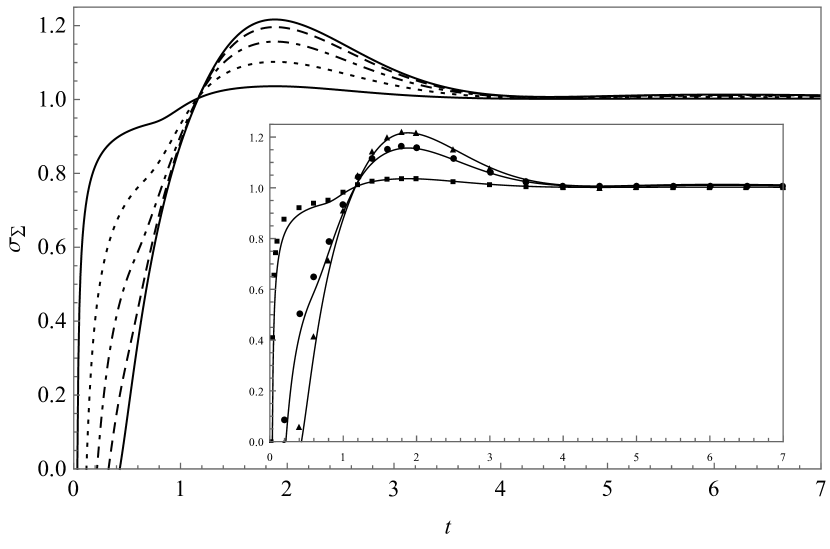
Figures 1 and 2 present displacements of several points of the rod for displacement of rod’s free end given as the Heaviside step function, i.e., for boundary condition (11)2 taken as The regularized solution kernel actually represents the step response, due to defining relation (19)2 for regularized solution kernel image that yields
after performing the inverse Laplace transform, see also (33).
The step response displays damped oscillatory behavior that settles at the value of point’s position, i.e.,
| (41) |
as predicted by the large-time asymptotics of regularized solution kernel given by (24). The time profiles of step response in the case of Model V have quite classical shapes of the oscillatory behavior with pronounced damping, see Figure 1a. On the other hand, the profiles in the case of Model VII, being also damped oscillatory, resemble to the sequence of excitation and relaxation processes, since profiles repeatedly change their convexity from concave to convex, as clearly visible from Figure 1b. Nevertheless, curves obtained by analytical expressions are consistent with curves represented by dots, that are obtained by numerical Laplace transform inversion using fixed Talbot method, see [1]. Regarding the short-time asymptotics, step response differs for Burgers models of the first and second class, since in the case of first class models time profiles continuously increase from zero, obtaining non-zero values depending on point’s position, see short-time asymptotics (22) of solution kernel and Figure 1a, while in the case of second class models time profiles jump from zero depending on point’s position, since the short-time asymptotics is represented by the Heaviside function, see (23) and Figure 1b.
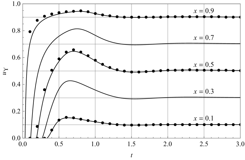
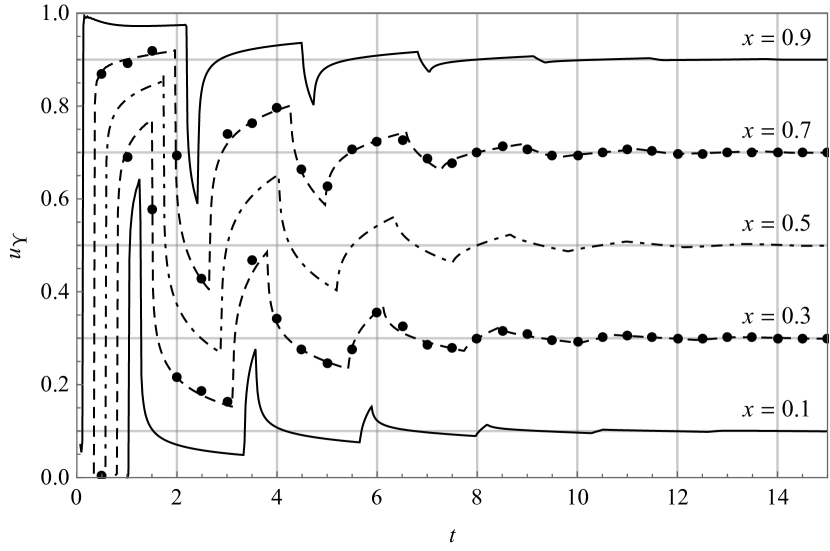
Plots from Figure 1 correspond to the case when solution kernel image and its regularization have no branch points except for so that the step responses are obtained using (30) with model parameters as in Table 1, while time profiles from Figure 2 correspond to the case when kernel image additionally has a pair of complex conjugated branch points with negative real part, hence the step responses are calculated by (32) using model parameters from Table 1. Although model parameters in the case of complex conjugated branch points do not satisfy narrowed thermodynamical restrictions, required in the proof that kernel image has a pair of complex conjugated poles this requirement is checked numerically, so as the fact that the argument of branch point is greater than the arguments of poles. Time profiles of the step response from Figure 2 are peculiarly shaped, as if two vibrations with different frequencies are superposed, since there is a relaxation process instead of peak, that is followed by another faster relaxation process, appearing after two successive excitation processes having different speeds. Moreover, responses have an envelope, that is typical for damped oscillations.
| Model | Branch points | |||||||||
| Model V | ||||||||||
| , , | ||||||||||
| Model VII | - | - |
Figures 3 and 4 present time profiles displaying stress at several points of the rod in the case of displacement of rod’s free end taken in the form of Heaviside step function, i.e., for as the boundary condition (11)2, so that, by (40), one has
| (42) |
In the case of Model V, as clearly visible from Figures 3a - 3c, step responses display damped oscillatory character, taking even negative values, with the pronounced first peak whose amplitude increases as positions are closer to rod’s free end, which is expected since the free end is subject to a sudden displacement. Note the good agreement between curves obtained through analytical expression and through ab initio numerical Laplace transform inversion. Time profiles in the case of Model VII resemble to a sequence of relaxation processes interrupted by sudden jumps decreasing in amplitude as time increases, see Figures 3d and 3e. Models V and VII differ in step responses regarding the short-time asymptotics, since in the case of Model V stress continuously increase from zero with significant rise depending on point’s position, as predicted by (37), while in the case of Model VII stress behaves as the Dirac delta distribution for small time, since by (38) and (42), as one has
Considering the large-time asymptotic of the step response, one starts from the Laplace transform of (42), with the solution kernel image given by (34) so that
| (43) |
because of the asymptotics of complex modulus given by (25). Note, the large-time asymptotics of the step response is exactly the same as for the relaxation modulus considered for constitutive equation solely, see Table 2 in [47].


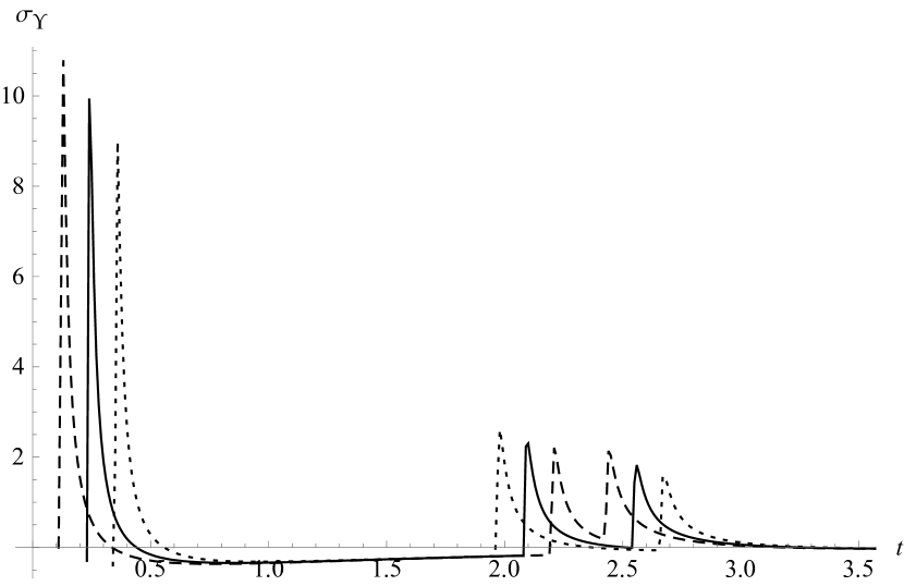


Contrary to the time profiles from Figure 3, that correspond to solution kernel image having no other branch points than responses presented in Figure 4 correspond to the case when solution kernel image has a pair of complex conjugated branch points with negative real part. Plots are produced for parameters given in Table 1, with regularization parameter . One notices that step response curves from Figure 4 are superpositions of curves similar to the ones from Figures 3a - 3c, whose shape does not depend on point’s position, and sequences of peaks whose position depends on point’s position. For small time, responses also resemble to the ones from Figures 3a - 3c, however they are not displayed in Figure 4 due to the large value of their amplitudes.
2.2 Solution for prescribed stress at rod’s free end
In the case of prescribed stress acting on rod’s free end, the Laplace transforms of displacement and stress, given by (16) and (17), are obtained as
| (44) |
since the function
is determined from the stress in the Laplace domain (17) and boundary condition (11)2.
2.2.1 Displacement for given
Displacement in the Laplace domain, given by (44)1, can be expressed through the solution kernel image , defined as
| (45) |
Considering the asymptotics of solution kernel image as one obtains
| (46) |
because of the asymptotics of complex modulus given by (21), so that the short-time asymptotics of solution kernel for models of the first class is obtained as
| (47) |
by inverting the Laplace transform of (46) using the definition and integration in the complex plane, while the short-time asymptotics of solution kernel corresponding to models of the second class yields
| (48) |
implying that the value of solution kernel for small time jumps from zero to a finite value at the time instant depending on the position and material properties.
On the other hand, the asymptotics of solution kernel image as yields
because of the asymptotics of complex modulus given by (25), implying that solution kernel for large time asymptotically tends to zero as the power type function, depending on the position
The solution kernel
| (49) |
is calculated by the definition of inverse Laplace transform similarly as the solution kernel see Section 3, using the Cauchy residues theorem, since complex valued function has infinite number of pairs of complex conjugated poles and for each lying in the left complex half-plane, each of them being poles of the first order, that are obtained as zeros of the denominator of function , i.e., as solutions of the equation
| (50) |
as proved in Section 4. As in the case of function function may also has branch points other than due to the square root of function The form of solution kernel given by (49), corresponds to the case of a pair of complex conjugated branch points and while its form corresponding to cases of no branch points or one negative real branch point is obtained by putting in (49).
2.2.2 Stress for given
Stress in the Laplace domain, given by (44)2, can be expressed either through the solution kernel image in the case of Burgers models of the first class, or through the regularized solution kernel in the case of the second class models, that are defined by
| (52) |
Considering the asymptotics of solution kernel image and its regularized version as by the asymptotics of complex modulus given by (21), one obtains
which has exactly the same form as the asymptotics of solution kernel image and its regularized version see (20), so that the short-time asymptotics of solution kernel for models of the first class is given by (22), while the asymptotics of corresponding models of the second class, is given by (23), i.e., by
| (53) | |||||
| (54) |
On the other hand, the asymptotics of regularized solution kernel image as yields
| (55) |
because of the asymptotics of complex modulus given by (25).
Using the regularized solution kernel the solution kernel reads
| (56) | |||||
similarly as in the case of solution kernel expressed through its regularization see (27).
The stress in the case of prescribed stress of rod’s free end is obtained as
| (57) |
by the inverse Laplace transform of (44), with solution kernel image defined by (52), where the solution kernel takes the form
| (58) |
in the case of models belonging to the first class, while in the case of the second model class, it is given by (56), with the regularized solution kernel being of the form
| (59) |
Solution kernel and its regularized version are obtained using the definition of the inverse Laplace transform, similarly as done in Section 3 when calculating the solution kernel . The form of solution kernels and correspond to the case when corresponding solution kernel image has a pair of complex conjugate branch points and in addition to while by putting in (58) and (59) one obtains their forms in cases when the image function has either no branch points or has one negative real branch point.
2.2.3 Numerical examples
Figures 5 and 6 present time profiles of displacement of several points of the rod for stress applied to rod’s free end assumed as the Heaviside step function, i.e., for boundary condition (11)3 taken as so that by (51), one has
| (60) |
The step response can be considered as a superposition of monotonically increasing curve and oscillations having amplitudes decreasing in time, that are quite pronounced in the case of the Model VII, see Figure 5b, while in the case of the Model V the oscillations cannot really be noticed, presumable due to large damping, see Figure 5a. Note the good agreement between curves obtained by analytical expression (60) and by the numerical Laplace transform inversion. The displacement tends to infinity for large time depending on point’s position, since the large-time asymptotics
| (61) |
is obtained from the Laplace transform of (60), with the solution kernel image given by (45), yielding
thanks to asymptotics of complex modulus , given by (25). The large-time asymptotics (61) implies that, depending on their position, all points of the rod have the same time behavior, that is exactly the same as for the creep compliance considered for constitutive equation, see Table 2 in [47]. As before, the step response differs for Burgers models of the first and second class, since time profiles continuously increase from zero in the case of Model V, see (47), while in the case of Model VII, according to the asymptotics of solution kernel image (46) and Laplace transform of (60), one has
implying that the short-time asymptotics of displacement has linear trend starting after In the case when solution kernel image has a pair of complex conjugated branch points, the step response curves, being non-smooth, are also damped oscillatory and superposed to monotonically increasing curves, see Figure 6. As before, plots are produced using the model parameters from Table 1.


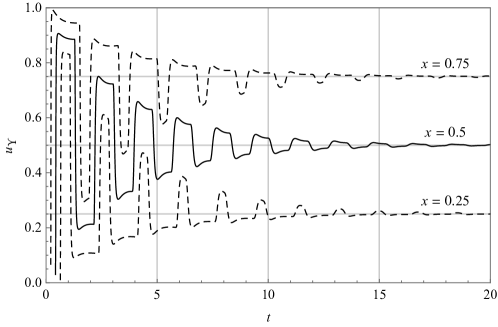
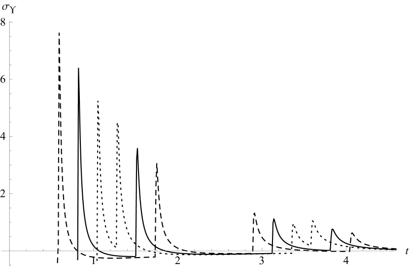
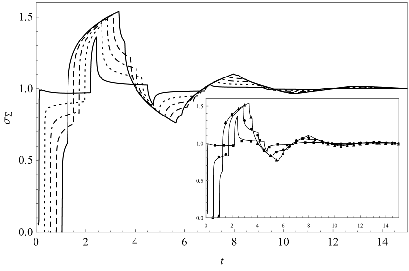
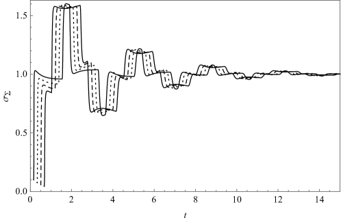
Figures 7 and 8 present time profiles displaying stress at several points of the rod for stress applied to rod’s free end assumed as the Heaviside step function, i.e., for boundary condition (11)3 taken as The regularized solution kernel actually represents the step response, due to defining relation (52)2 for regularized solution kernel image that yields
after performing the inverse Laplace transform, see also (57).
The behavior of step response is of the damped oscillatory type, that settles at the value of stress applied to rod’s free end, i.e.,
| (62) |
as predicted by the large-time asymptotics of regularized solution kernel given by (55). The time profiles of step response in the case of Model V display oscillatory behavior with the very pronounced damping, see Figure 7a. On the other hand, the profiles in the case of Model VII, being also damped oscillatory, resemble to the sequence of two excitation processes followed by two relaxation processes, since profiles repeatedly change their convexity from concave to convex, as clearly visible from Figure 7b. Again, good agreement between curves obtained analytically through (59), using parameters from Table 1, and by ab initio numerical Laplace transform inversion is observed. Step response differs for Models V and VII regarding the short-time asymptotics, since in the case of Model V time profiles continuously increase from zero, obtaining non-zero values depending on point’s position, see (53) and Figure 7a, while for Model VII time profiles jump from zero depending on point’s position, due to the Heaviside function as the short-time asymptotics, see (54) and Figure 7b.
Contrary to the case of plots from Figure 7, that correspond to the case when solution kernel image and its regularization have no other branch points than time profiles from Figure 8 correspond to the case when kernel image additionally has a pair of complex conjugated branch points. Time profiles presented in Figure 8 are peculiarly shaped, as if several damped vibrations with different frequencies are superposed. Responses seem to have an envelope, that is typical for damped oscillations.
3 Calculation of solution kernel
In order to obtain the solution kernel in the form (29), the inverse Laplace transform formula is applied to solution kernel image , given by (19)1, yielding
where the integration is performed along the Bromwich path , that is obtained from the contour in the limit as , with the contour being the part of the closed contour: if function does not have branch points other than if function has a negative real branch point in addition to , and if function has a pair of complex conjugated branch points in addition to respectively shown in Figures 9, 10, and 11. Each of the contours and are used in the Cauchy residues theorem
| (63) |
where all poles of function lie in the domain encircled by contour in the limit when and .
The branch points of solution kernel image are due to the complex modulus since, by (13), it contains function given by (14)1 for the first class of the Burgers models and by (15)1 for the second class models, that
|
where
with determined from
for Models I - VII, while in the case of Model VIII function
|
where and as proved in [47].
3.1 Case when function has no branch points other than
In the case when solution kernel image has no branch points other than the integrals along contours , , and belonging to the integration contour from Figure 9 and appearing in the Cauchy residues theorem (63), have non-zero contribution and according to contours’ parameterization given in Table 2, in the limit when and take the form
| (64) | |||||
| (65) | |||||
| (66) |
where the notation
| (67) |
is used, while the integrals along all other contours have zero contribution when and as will be proved below.
![[Uncaptioned image]](/html/2103.07175/assets/x19.png)
| Bromwich path, | ||
| arbitrary, | ||
| arbitrary. |
The residues in theorem (63), calculated according to
| (68) |
where and where , , are poles of the first order of function , see (19)1, lying in the upper left complex quarter-plane as proved in Section 4, become
when (28) is used in (68). The complex conjugation of equation (28) gives
implying , where is the complex conjugate of , so that the right hand side of the Cauchy residues theorem (63) becomes
| (69) | |||
| (70) |
where , . Note, the last term in (69) is zero since
due to as , according to the equation (28).
Summing up, the integrals having non-zero contribution (64), (65), and (66), as well as the residues (70), according to the Cauchy residues theorem (63) yield
| (71) |
It is left to prove that the integrals along contours and tend to zero in the limit and . Regardless of the fact that the form (71) of solution kernel is only valid for models of the first class, in showing zero contributions of the mentioned integrals, models of the second class will be also addressed, since the regularized solution kernel is treated analogously.
The integral along the contour according to its parameterization from Table 2, is
so that
due to the asymptotic behavior
with , implying in the case of the first class of Burgers models, while in the case of the second class of Burgers models, the expression (3.1) becomes
since due to the asymptotics
found by applying formulae and to
that are obtained by (86) and (87), since by (77) it holds as . Therefore, the integral when , and by similar arguments integral when .
Using the parameterization from Table 2, the integral along contour takes the form
so that
| (73) | |||||
In the case of the first class of Burgers models, the asymptotic behavior of on contour is
where , implying , so it is necessary to consider two intervals: since then and since then with Therefore, the expression (73) become
For the Burgers models of the second class the expression (73) gives
due to the asymptotics
So, when , and using a similar argumentation when
Integral on the contour parameterized using parameterization given in Table 2, is
so that
with , since for the Burgers models of both classes the following asymptotics holds
where for small is additionally used.
3.2 Case when function has negative real branch point in addition to
In the case when solution kernel image has a negative real branch point in addition to the integration in the Cauchy residues theorem (63) is performed along the contour shown in Figure 10, and, as in the previous case, the integrals along contours , , and have non-zero contribution and according to contours’ parameterization given in Table 3 take the same form as given by (64), (65), and (66). In addition to the integrals, the residues are also already calculated in Section 3.1 and given by (70). Solution kernel takes the form (71), since, as in the case when function has no other branch points than , the integrals along contours and have zero contribution, as already proved in Section 3.1, so it is left to prove that the integrals along the contours and have zero contributions.
![[Uncaptioned image]](/html/2103.07175/assets/x20.png)
| Bromwich path, | ||
| arbitrary, | ||
| arbitrary, | ||
| . |
Integral on the contour parameterized using parameterization given in Table 3, by (67) is
so that
where for small is additionally used, since the asymptotics
holds for the Burgers models of both classes because
| (75) |
see equation (B.31) in [47], implying
with By the similar arguments the integral also tends to zero as .
3.3 Case when function has a pair of complex conjugated branch points in addition to
In the case when solution kernel image in addition to has a pair of complex conjugated branch points and having negative real part, with assuming that the absolute value of poles’ argument is less then the argument of branch points, the integration in the Cauchy residues theorem (63) is performed along the contour shown in Figure 11, so that the integrals along contours , , and have non-zero contribution and according to contours’ parameterization given in Table 4 by (67) take the following forms
while the residues are already calculated in Section 3.1 and given by (70), so that the solution kernel takes the form
| (76) |
since the integrals along all other contours are zero. It is already proved in Section 3.1 that the integrals along contours and have zero contribution, so it is left to prove that the integrals along the contours and have zero contributions as well.
![[Uncaptioned image]](/html/2103.07175/assets/x21.png)
| Bromwich path, | ||
| arbitrary, | ||
| arbitrary, | ||
| . |
Integral on the contour parameterized using parameterization given in Table 4, by (67) is
so that
where for small is additionally used, since the asymptotics
holds for the Burgers models of both classes, because
that is obtained similarly as (75) implies
with By the similar arguments the integral also tends to zero as .
4 Zeros of function
In order to obtain poles of functions and according to equations (28) and (50), one needs to examine the position, number, and multiplicity of zeros of function , defined by
| (77) |
Although equation (77) cannot be solved analytically, it will be proved that function , defined by (77), for each has a pair of complex conjugated zeros having negative real part, representing poles of functions and
Introducing the substitution into function given by (77), its real and imaginary parts become
| (78) | |||||
| (79) |
with for the first, respectively for the second class of Burgers models, where functions and are given by
| (80) | |||||
for the first class and by
| (81) | |||||
for the second class. Note that according to the thermodynamical restrictions.
If is a zero of function then its complex conjugate is a zero as well, since according to (79), hence it is sufficient to seek for zeros of function in the upper complex half-plane only. Moreover, as proved in Appendix A of [48], function does not have zeros in the right complex half-plane and therefore in order to have a pair of complex conjugated zeros of lying in the left half-plane it is left to prove using the argument principle and contour shown in Figure 12 along with its parameterization given in Table 5, that the zeros of lie in the upper left complex quarter-plane. Recall, the argument principle claims that if the variable changes along the contour closed in the complex plane, then the number of zeros of function in the domain encircled by contour is given by provided that function does not have poles in the mentioned domain.
![[Uncaptioned image]](/html/2103.07175/assets/x22.png)
The argument of complex numbers belonging to the contour has a fixed value while their modulus changes so that implying the real and imaginary parts of function given by (78) and (79), in the form
| (82) | |||||
| (83) |
since all terms in are positive, see (80) and (81). The asymptotics of (82) and (83) for both model classes as yields
while the asymptotics as for the first model class gives
| (84) | |||||
| (85) |
since by the thermodynamic requirements as well as
| (86) | |||||
| (87) |
for the second model class. From the asymptotics (84) and (85) it follows that and implying with while form the asymptotics (86) and (87) it follows that and implying . In conclusion, as changes along the contour the argument of function changes from zero either to in the case of Burgers models of the first class, or to in the case of models of the second class.
Complex number lying on the contour has large but fixed modulus while its argument changes along the contour taking the values so that the asymptotics of (78) and (79) as in the case of Burgers models belonging to the first class gives
| (88) | |||||
| (89) |
as well as
| (90) | |||||
| (91) |
for the Burgers models belonging to the second class, where the second term in disappears for but has a dominant role if or Therefore, real and imaginary parts of function cannot be simultaneously positive for since in the case of Models I, III, and IV, as well as in the case of Models II and V, and obviously for models of the second class. If then (88) and (89) reduce to (84) and (85), so as (90) and (91) to (86) and (87), while if then (88) and (89) become
| (92) | |||||
| (93) |
| (94) | |||||
| (95) |
Therefore, as changes along contour , the argument of function changes through the second, third, and possibly fourth quadrant.
The argument of complex numbers lying on the contour has a fixed value while their modulus changes in the interval yielding
| (96) | |||||
| (97) |
for the real and imaginary parts of the function since for due to the conditions narrowing thermodynamical restrictions in the case of all fractional Burgers models, which is proved for each model separately. In the case of Model I, function obtained in the form
by (80), is positive due to the narrowed thermodynamical restrictions (102). In the case of Model II, function obtained as
is positive due to the narrowed thermodynamical restrictions (104). In the case of Model III, function obtained as
by (80), is positive due to the narrowed thermodynamical restrictions (106). In the case of Model IV, function obtained as
by (80), is positive due to the narrowed thermodynamical restrictions (108). In the case of Model V, function obtained as
by (80), is positive due to the narrowed thermodynamical restrictions (110). In the case of Model VI, function obtained as
by (81), is positive due to the narrowed thermodynamical restrictions (112). In the case of Model VII, the positivity of function obtained as
by (81), is achieved by requiring the positivity of the trinomial quadratic in that is guaranteed by the narrowed thermodynamical restrictions (114). In the case of Model VIII, the positivity of function obtained as
by (81), is achieved by requiring the positivity of the trinomial quadratic in that is guaranteed by the narrowed thermodynamical restrictions (116). The asymptotics as of the real and imaginary parts of function given by (96) and (97), reduce to (92) and (93) for the Burgers models of the first class, as well as to (94) and (95) for the Burgers models of the second class, while for the real and imaginary parts of function become
| (99) | |||||
| (100) |
Hence, as changes along contour , by (97) and (100), imaginary part of function is negative and as by (99), the real part of function tends to
The modulus of complex numbers belonging to the contour has a fixed but small value while their argument changes in the interval so that (78) and (79) become
implying that regardless of the sign of , the function remains in the neighborhood of a finite positive number .
Summing up, the change of argument of function is as changes along the contour implying that function has one zero in the upper left complex quarter-plane for each
5 Conclusion
The fractional Burgers wave equation, written as the system of equations consisting of the equation of motion and strain (1), that are coupled either with Burgers models of the first class (2) or with models of the second class (3), is used to model the dynamic response of the initially undisturbed one-dimensional viscoelastic rod of finite length having one end fixed and the other subject to prescribed either displacement or stress, according to boundary conditions (5). Laplace transform method is used in order to express the displacement and stress of an arbitrary rod’s point in terms of boundary condition convoluted with the solution kernel.
The short-time asymptotics of solution kernels implied that their time profiles continuously increase from zero as time increases, with the significant rise depending on the point’s position in the case of Burgers models of the first class, see short-time asymptotics for solution kernels and given by (23), (38), (47), and (53), respectively, implying the infinite wave propagation speed. On the other hand, solution kernels and corresponding to the Burgers models of the second class, have to be regularized, so that the short-time asymptotics of and is the Heaviside function of the argument see (23) and (54), implying the finite wave propagation speed , due to the sudden jump in the value of and at Solution kernel is regularized differently, implying that for small time its regularization behaves as the time derivative of the Dirac delta regularization, calculated at see (38). It is noteworthy that the regularization of solution kernel is not necessary, since its short-time asymptotics is the Heaviside function of the argument see (48).
All solution kernels consist of two terms: the integral one is at most non-monotonic in both space and time and the one expressed either through the sine or cosine Fourier series represents a superposition of standing waves, each of them oscillating with amplitude decreasing in time, having the damping and angular frequency determined by the pole of the solution kernel image. Moreover, the form of solution kernel also depends on occurrence of branch points of solution kernel image.
Time profiles of the displacement and stress step responses are of quite classical shapes corresponding to the damped oscillatory behavior in the case of Burgers models of the first class, while in the case of the second class models, the time profiles are peculiarly shaped resembling to the sequence of excitation and relaxation processes. Nevertheless, the large-time asymptotics of the step response for prescribed displacement of rod’s free end yielded
while in the case of prescribed stress acting on rod’s free end, one has
see (7)2, (41), (43), (61), and (62), respectively, that is in a perfect accordance with the behavior of relaxation modulus and creep compliance, studied in [47] for the thermodynamically consistent fractional Burgers models.
Acknowledgment
This work is supported by the Serbian Ministry of Science, Education and Technological Development under grant 451-03-9/2021-14/200125 (DZ).
Appendix A Fractional Burgers models
Thermodynamically consistent fractional Burgers models are listed below, along with corresponding thermodynamical constraints, as well as with the constraints on monotonicity of relaxation modulus and creep compliance, narrowing down the thermodynamical requirements and guaranteeing that relaxation modulus is completely monotonic, while creep compliance is Bernstein function.
Model I:
| (101) | |||
| (102) |
with
Model II:
| (103) | |||
| (104) |
Model III:
| (105) | |||
| (106) |
Model IV:
| (107) | |||
| (108) |
Model V:
| (109) | |||
| (110) |
Model VI:
| (111) | |||
| (112) |
Model VII:
| (113) | |||
| (114) |
Model VIII:
| (115) | |||
| (116) |
References
- [1] J. Abate and P. P. Valkó. Multi-precision Laplace transform inversion. International Journal for Numerical Methods in Engineering, 60:979–993, 2004.
- [2] A. Abbas, E. Masad, T. Papagiannakis, and T. Harman. Micromechanical modeling of the viscoelastic behavior of asphalt mixtures using the discrete-element method. International Journal of Geomechanics, 7:131–139, 2007.
- [3] T. M. Atanackovic, M. Janev, and S. Pilipovic. On the thermodynamical restrictions in isothermal deformations of fractional Burgers model. Philosophical Transactions of the Royal Society A, 378:20190278–1–13, 2020.
- [4] T. M. Atanackovic, S. Konjik, Lj. Oparnica, and D. Zorica. Thermodynamical restrictions and wave propagation for a class of fractional order viscoelastic rods. Abstract and Applied Analysis, 2011:ID975694–1–32, 2011.
- [5] T. M. Atanackovic, S. Pilipovic, B. Stankovic, and D. Zorica. Fractional Calculus with Applications in Mechanics: Vibrations and Diffusion Processes. Wiley-ISTE, London, 2014.
- [6] T. M. Atanackovic, S. Pilipovic, B. Stankovic, and D. Zorica. Fractional Calculus with Applications in Mechanics: Wave Propagation, Impact and Variational Principles. Wiley-ISTE, London, 2014.
- [7] T. M. Atanackovic, S. Pilipovic, and D. Zorica. Distributed-order fractional wave equation on a finite domain: creep and forced oscillations of a rod. Continuum Mechanics and Thermodynamics, 23:305–318, 2011.
- [8] T. M. Atanackovic, S. Pilipovic, and D. Zorica. Distributed-order fractional wave equation on a finite domain. Stress relaxation in a rod. International Journal of Engineering Science, 49:175–190, 2011.
- [9] E. Bazhlekova and I. Bazhlekov. Complete monotonicity of the relaxation moduli of distributed-order fractional Zener model. In Proceedings of the 44 International Conference on Applications of Mathematics in Engineering and Economics, AIP Conference Proceedings 2048, pages 050008–1–8, 2018.
- [10] E. Bazhlekova and K. Tsocheva. Fractional Burgers’ model: thermodynamic constraints and completely monotonic relaxation function. Comptes rendus de l’Académie bulgare des Sciences, 69:825–834, 2016.
- [11] P. W. Buchen and F. Mainardi. Asymptotic expansions for transient viscoelastic waves. Journal de mécanique, 14:597–608, 1975.
- [12] W. Cai, W. Chen, J. Fang, and S. Holm. A survey on fractional derivative modeling of power-law frequency-dependent viscous dissipative and scattering attenuation in acoustic wave propagation. Applied Mechanics Reviews, 70:1–12, 2018.
- [13] C. Celauro, C. Fecarotti, A. Pirrotta, and A. C. Collop. Experimental validation of a fractional model for creep/recovery testing of asphalt mixtures. Construction and Building Materials, 36:458–466, 2012.
- [14] I. Colombaro, A. Giusti, and F. Mainardi. A class of linear viscoelastic models based on Bessel functions. Meccanica, 52:825–832, 2017.
- [15] I. Colombaro, A. Giusti, and F. Mainardi. On the propagation of transient waves in a viscoelastic bessel medium. Zeitschrift für angewandte Mathematik und Physik, 68:62–1–13, 2017.
- [16] I. Colombaro, A. Giusti, and F. Mainardi. On transient waves in linear viscoelasticity. Wave Motion, 74:191–212, 2017.
- [17] N. Demi̇rci̇ and E. Tönük. Non-integer viscoelastic constitutive law to model soft biological tissues to in-vivo indentation. Acta of Bioengineering and Biomechanics, 16:14–21, 2014.
- [18] A. Giusti and F. Mainardi. A dynamic viscoelastic analogy for fluid-filled elastic tubes. Meccanica, 51:2321–2330, 2016.
- [19] N. M. Grahovac and M. M. Žigić. Modelling of the hamstring muscle group by use of fractional derivatives. Computers and Mathematics with Applications, 59:1695–1700, 2010.
- [20] A. Hanyga. Wave propagation in linear viscoelastic media with completely monotonic relaxation moduli. Wave Motion, 50:909–928, 2013.
- [21] A. Hanyga. Attenuation and shock waves in linear hereditary viscoelastic media; Strick-Mainardi, Jeffreys-Lomnitz-Strick and Andrade creep compliances. Pure and Applied Geophysics, 171:2097–2109, 2014.
- [22] A. Hanyga. Dispersion and attenuation for an acoustic wave equation consistent with viscoelasticity. Journal of Computational Acoustics, 22:1450006–1–22, 2014.
- [23] A. Hanyga. Asymptotic estimates of viscoelastic Green’s functions near the wavefront. Quarterly of Applied Mathematics, 73:679–692, 2015.
- [24] A. Hanyga. Effects of Newtonian viscosity and relaxation on linear viscoelastic wave propagation. Archive of Applied Mechanics, 2019.
- [25] N. Heymans. Hierarchical models for viscoelasticity dynamic behaviour in the linear range. Rheologica Acta, 35:508–519, 1996.
- [26] S. Holm. Waves with Power-Law Attenuation. Springer Nature Switzerland AG, Cham, 2019.
- [27] S. Hyder Ali Muttaqi Shah. Some helical flows of a Burgers’ fluid with fractional derivative. Meccanica, 45:143–151, 2010.
- [28] S. Hyder Ali Muttaqi Shah. Unsteady flows of a viscoelastic fluid with the fractional Burgers’ model. Nonlinear Analysis: Real World Applications, 11:1714–1721, 2010.
- [29] S. Hyder Ali Muttaqi Shah and H. Qi. Starting solutions for a viscoelastic fluid with fractional Burgers’ model in an annular pipe. Nonlinear Analysis: Real World Applications, 11:547–554, 2010.
- [30] M. Jamil and C. Fetecau. Some exact solutions for rotating flows of a generalized Burgers’ fluid in cylindrical domains. Journal of Non-Newtonian Fluid Mechanics, 165:1700–1712, 2010.
- [31] J. Kang, Y. Liu, and T. Xia. Unsteady flows of a generalized fractional Burgers’ fluid between two side walls perpendicular to a plate. Advances in Mathematical Physics, 2015:521069–1–9, 2015.
- [32] M. Khan, A. Anjum, C. Fetecau, and H. Qi. Exact solutions for some oscillating motions of a fractional Burgers’ fluid. Mathematical and Computer Modelling, 51:682–692, 2010.
- [33] M. Khan, S. Hyder Ali, and H. Qi. Exact solutions of starting flows for a fractional Burgers’ fluid between coaxial cylinders. Nonlinear Analysis: Real World Applications, 10:1775–1783, 2009.
- [34] M. Khan, S. Hyder Ali, and H. Qi. On accelerated flows of a viscoelastic fluid with the fractional Burgers’ model. Nonlinear Analysis: Real World Applications, 10:2286–2296, 2009.
- [35] A. A. Kilbas, H. M. Srivastava, and J. J. Trujillo. Theory and Applications of Fractional Differential Equations. Elsevier B.V., Amsterdam, 2006.
- [36] Y. R. Kim. Modeling of Asphalt Concrete. McGraw-Hill, New York, 2009.
- [37] S. Konjik, Lj. Oparnica, and D. Zorica. Distributed-order fractional constitutive stress-strain relation in wave propagation modeling. Zeitschrift für angewandte Mathematik und Physik, 70:51–1–21, 2019.
- [38] Y. Liu, Q. Dai, and Z. You. Viscoelastic model for discrete element simulation of asphalt mixtures. Journal of Engineering Mechanics, 135:324–333, 2009.
- [39] Y. Luchko and F. Mainardi. Some properties of the fundamental solution to the signalling problem for the fractional diffusion-wave equation. Central European Journal of Physics, 11:666–675, 2013.
- [40] Y. Luchko and F. Mainardi. Cauchy and signaling problems for the time-fractional diffusion-wave equation. Journal of Vibration and Acoustics, 136:050904–1–7, 2014.
- [41] Y. Luchko, F. Mainardi, and Y. Povstenko. Propagation speed of the maximum of the fundamental solution to the fractional diffusion-wave equation. Computers and Mathematics with Applications, 66:774–784, 2013.
- [42] F. Mainardi. Fractional Calculus and Waves in Linear Viscoelasticity. Imperial College Press, London, 2010.
- [43] F. Mainardi and G. Spada. Creep, relaxation and viscosity properties for basic fractional models in rheology. European Physical Journal Special Topics, 193:133–160, 2011.
- [44] N. Makris. The frequency response function of the creep compliance. Meccanica, 54:19–31, 2019.
- [45] M. Oeser, T. Pellinen, T. Scarpas, and C. Kasbergen. Studies on creep and recovery of rheological bodies based upon conventional and fractional formulations and their application on asphalt mixture. International Journal of Pavement Engineering, 9:373–386, 2008.
- [46] A. S. Okuka and D. Zorica. Formulation of thermodynamically consistent fractional Burgers models. Acta Mechanica, 229:3557–3570, 2018.
- [47] A. S. Okuka and D. Zorica. Fractional Burgers models in creep and stress relaxation tests. Applied Mathematical Modelling, 77:1894–1935, 2020.
- [48] Lj. Oparnica, D. Zorica, and A. S. Okuka. Fractional Burgers wave equation. Acta Mechanica, 230:4321–4340, 2019.
- [49] Yu. A. Rossikhin and M. V. Shitikova. Analysis of dynamic behavior of viscoelastic rods whose rheological models contain fractional derivatives of two different orders. Zeitschrift für angewandte Mathematik und Mechanik, 81:363–376, 2001.
- [50] Yu. A. Rossikhin and M. V. Shitikova. Analysis of rheological equations involving more than one fractional parameters by the use of the simplest mechanical systems based on these equations. Mechanics of Time-Dependent Materials, 5:131–175, 2001.
- [51] Yu. A. Rossikhin and M. V. Shitikova. A new method for solving dynamic problems of fractional derivative viscoelasticity. International Journal of Engineering Science, 39:149–176, 2001.
- [52] Yu. A. Rossikhin and M. V. Shitikova. Analysis of the viscoelastic rod dynamics via models involving fractional derivatives or operators of two different orders. Shock and Vibration Digest, 36:3–26, 2004.
- [53] Yu. A. Rossikhin and M. V. Shitikova. Free damped vibrations of a viscoelastic oscillator based on Rabotnov’s model. Mechanics of Time-Dependent Materials, 12:129–149, 2008.
- [54] Yu. A. Rossikhin and M. V. Shitikova. Application of fractional calculus for dynamic problems of solid mechanics: Novel trends and recent results. Applied Mechanics Reviews, 63:010801–1–52, 2010.
- [55] B. Wu. On seismic wave propagation through subsurface media. European Physical Journal Plus, 134:357–1–8, 2019.
- [56] H. Xu and X. Jiang. Creep constitutive models for viscoelastic materials based on fractional derivatives. Computers and Mathematics with Applications, 73:1377–1384, 2017.
- [57] A. Zbiciak. Mathematical description of rheological properties of asphalt-aggregate mixes. Bulletin of the Polish Academy of Sciences Technical Sciences, 61:65–72, 2013.
- [58] T. Zhou, J. Yan, J. Masuda, and T. Kuriyagawa. Investigation on the viscoelasticity of optical glass in ultraprecision lens molding process. Journal of Materials Processing Technology, 209:4484–4489, 2009.
- [59] D. Zorica and Lj. Oparnica. Energy dissipation for hereditary and energy conservation for non-local fractional wave equations. Philosophical Transactions of the Royal Society A, 378:20190295–1–24, 2020.