Max-Linear Regression by Scalable and Guaranteed Convex Programming

Abstract

We consider the multivariate max-linear regression problem where the model parameters $\bm{\beta}_{1},\dotsc,\bm{\beta}_{k}\in\mathbb{R}^{p}$ need to be estimated from $n$ independent samples of the (noisy) observations $y=\max_{1\leq j\leq k}\bm{\beta}_{j}^{\mathsf{T}}\bm{x}+\mathrm{noise}$. The max-linear model vastly generalizes the conventional linear model, and it can approximate any convex function to an arbitrary accuracy when the number of linear models $k$ is large enough. However, the inherent nonlinearity of the max-linear model renders the estimation of the regression parameters computationally challenging. Particularly, no estimator based on convex programming is known in the literature. We formulate and analyze a scalable convex program as the estimator for the max-linear regression problem. Under the standard Gaussian observation setting, we present a non-asymptotic performance guarantee showing that the convex program recovers the parameters with high probability. When the $k$ linear components are equally likely to achieve the maximum, our result shows that a sufficient number of observations scales as $k^{2}p$ up to a logarithmic factor. This significantly improves on the analogous prior result based on alternating minimization (Ghosh et al., 2019). Finally, through a set of Monte Carlo simulations, we illustrate that our theoretical result is consistent with empirical behavior, and the convex estimator for max-linear regression is as competitive as the alternating minimization algorithm in practice.
Keywords: nonlinear regression, convex programming, max-linear model, empirical processes, and sample complexity

1 Introduction

We consider the problem of estimating the parameters $\bm{\beta}_{\star,1},\dotsc,\bm{\beta}_{\star,k}\in\mathbb{R}^{p}$ that determine the max-linear function

$$\bm{x}\in\mathbb{R}^{p}\mapsto\max_{j\in[k]}\ \langle\bm{\beta}_{\star,j},\bm{x}\rangle\,,$$ (1.1)

from independent and identically distributed (i.i.d.) observations, where $[k]$ denotes the set $\{1,\dots,k\}$. Specifically, given the data points $\bm{x}_{1},\dotsc,\bm{x}_{n}\in\mathbb{R}^{p}$, and denoting the value of a max-linear function, with parameter $\bm{\beta}$, at these points by

$$f_{i}(\bm{\beta})\stackrel{{\scriptstyle\textup{\tiny def}}}{{=}}\max_{j\in[k]}\ \langle\bm{x}_{i},\bm{\beta}_{j}\rangle\,,$$ (1.2)

we observe the nonlinear measurement

$$y_{i}=f_{i}(\bm{\beta}_{\star})+w_{i}\,,$$

of the parameter vector $\bm{\beta}_{\star}=[\bm{\beta}_{\star,1};\,\dotsc\,;\bm{\beta}_{\star,k}]\in\mathbb{R}^{kp}$ where $w_{i}$ denotes noise for $i\in[n]$.

The closest result in the literature to ours is that of Ghosh et al. (2019), which studies the slightly more general problem of max-affine regression and considers an alternating minimization approach as the estimator. Each iteration of this alternating minimization approach basically consists in a step for identifying the maximizing linear terms, and a following step of solving least squares to estimate the corresponding parameters. However, the theoretical and empirical performance of (Ghosh et al., 2019) critically depends on the level of the observation noise, mainly due to the sensitivity of the “maximizer identification” step in each iteration of the algorithm. Leveraging recent theory for convexifying nonlinear inverse problems in the original domain (Bahmani and Romberg, 2017; Bahmani, 2019; Bahmani and Romberg, 2019), we propose an alternative approach by convex programming. Due to the inherent geometry of the formulation, the convex estimator provides stable performance in the presence of noise. It is worth mentioning that (Ghosh et al., 2019) considered a random noise model and analyzed the accuracy in terms of the noise variance, whereas we consider the deterministic “gross error” model. Nevertheless, in the noiseless case, both results essentially achieve the same sample complexity.

1.1 Convex estimator

The common estimators for $\bm{\beta}_{\star}$ such as the least absolute deviation (LAD), i.e.,

$$\mathop{\mathrm{minimize}}_{\bm{\beta}}~{}\frac{1}{n}\sum_{i=1}^{n}\left|f_{i}(\bm{\beta})-y_{i}\right|\,,$$ (1.3)

are generally hard to compute as they involve a nonconvex optimization. Given an “anchor vector” $\bm{\theta}$, we study the estimation of $\bm{\beta}_{\star}$ through anchored regression that formulates the estimation by the convex program

$$\begin{array}[]{ll}\displaystyle\mathop{\mathrm{maximize}}_{\bm{\beta}}&\langle\bm{\theta},\bm{\beta}\rangle\\ \mathrm{subject~{}to}&\displaystyle\frac{1}{n}\sum_{i=1}^{n}\left(f_{i}(\bm{\beta})-y_{i}\right)_{+}\leq\eta\,,\end{array}$$ (1.4)

where $(\cdot)_{+}$ denotes the positive part function and $\eta=\frac{1}{n}\sum_{i=1}^{n}(-w_{i})_{+}$. The anchored regression can be interpreted as a convexification of the LAD estimator. Since the observation functions (1.2) are convex, the LAD is nonconvex mainly due to the effect of the absolute value operator in (1.3). This source of nonconvexity is removed in anchored regression by relaxing the absolute deviation to the positive part of the error. The linear objective that is determined by the anchor vector $\bm{\theta}$ acts as a “regularizer” to prevent degenerate solutions and guarantees exact recovery of the true parameter $\bm{\beta}_{\star}$ under certain conditions on the measurement model in the noiseless scenario.

Anchored regression has been originally developed as a scalable convex program to solve the phase retrieval problem (Bahmani and Romberg, 2017; Goldstein and Studer, 2018) with provable guarantees. Anchored regression is highly scalable compared to other convex relaxations in this context (Candes et al., 2013; Waldspurger et al., 2015) that rely on semidefinite programming. The idea of anchored regression is further studied in a broader class of nonlinear parametric regression problems with convex observations (Bahmani and Romberg, 2019) and difference of convex functions (Bahmani, 2019).

1.2 Background and motivation

A closely related problem is the max-affine regression problem. A max-affine model generalizes the max-linear model in (1.1) by introducing an extra offset parameter to each component. Alternatively, by fixing any regressor to constant $1$, each linear component in (1.1) has its range away from the origin, which turns the model into a max-affine model. Thus methods developed for the two models are compatible. For the sake of simplicity, we use the description in (1.1). If necessary, a coordinate of $\bm{x}_{i}$ can be fixed to $1$ for all $i\in[n]$.

Since max-affine model can approximate a convex function to an arbitrary accuracy, it has been utilized in numerous applications, particularly in machine learning and optimization. Recently it has been shown that an extension called max-affine spline operators (MASOs) can represent a large class of deep neural networks (DNNs) (Balestriero and Baraniuk, 2018; Balestriero et al., 2019, 2020). They leveraged the model to analyze the expressive power of various DNNs. Max-affine model has also been leveraged to approximate Bregeman divergences in metric learning (Siahkamari et al., 2019) and utility functions in energy storage and beer brewery optimization problems (Balázs, 2016).

As mentioned above, the estimation for max-affine or max-linear regression is challenging due to the inherent nonlinearity in the model. In the literature, the max-affine regression problem has been studied mostly as a nonlinear least squares (Magnani and Boyd, 2009; Toriello and Vielma, 2012; Hannah and Dunson, 2013; Balázs, 2016; Ghosh et al., 2019; Ho et al., 2019):

$$\widehat{\bm{\beta}}=\operatorname*{argmin}_{[\bm{\beta}_{1};\dots;\bm{\beta}_{k}]}\sum_{i=1}^{n}\left(\max_{1\leq j\leq k}\langle\bm{x}_{i},\bm{\beta}_{j}\rangle-\bm{y}_{i}\right)^{2}\,.$$ (1.5)

By utilizing a special structure in (1.5), a suite of alternating minimization algorithms have been developed (Magnani and Boyd, 2009; Toriello and Vielma, 2012; Hannah and Dunson, 2013). The fact that (1.1) is a special case of piecewise linear function allows us to divide $\bm{x}_{1},\ldots,\bm{x}_{n}$ into $k$ partitions based on their membership in the polyhedral cones

$$\mathcal{C}_{j}\stackrel{{\scriptstyle\textup{\tiny def}}}{{=}}\left\{\bm{w}\in\mathbb{R}^{p}~{}:~{}\left\langle\bm{w},\bm{\beta}_{\star,j}-\bm{\beta}_{\star,l}\right\rangle\geq 0,~{}\forall l\neq j\right\}\,,\quad j\in[k]\,,$$ (1.6)

that are pairwise almost disjoint and cover the entire space $\mathbb{R}^{p}$. In other words, $\mathcal{C}_{j}$ is determined according to which component achieves the maximum in the max-linear model in (1.1). If this oracle information is known a priori, then the estimation is divided into $k$ decoupled linear least squares given by

$$\widehat{\bm{\beta}}_{j}=\operatorname*{argmin}_{\bm{\beta}_{j}}\sum_{i\in\mathcal{C}_{j}}\left(\langle\bm{x}_{i},\bm{\beta}_{j}\rangle-\bm{y}_{i}\right)^{2},\quad j\in[k]\,.$$

Magnani and Boyd (2009) proposed the least-square partition algorithm (LSPA), which progressively refine estimates for both $\{\bm{\beta}_{\star,j}\}_{j=1}^{k}$ and $\{\mathcal{C}_{j}\}_{j=1}^{k}$, which is a reminiscent of the $k$-means clustering algorithm. Hannah and Dunson (2013) proposed the convex adaptive partitioning (CAP) method by applying the adaptive partitioning technique that splits and refines the partitions. The CAP method exploits the adaptive partitioning technique which divides partitions with respect to coordinate $u\in[p]$ and selecting the only partition which minimizes the mean square error on the observations $(\bm{x}_{i},y_{i}),i\in[n]$. By selecting this adaptive partition method which is improved version of naive partitioning method used in LSPA, they showed improved performance in empirical result. Later, Balázs (2016) proposed the adaptive max-affine partitioning algorithm (AMAP) that exploits both LSPA and the CAP method with a cross-validation scheme. By applying the adaptive partition method in CAP but replacing the partition criterion by partitioning at median, they reduced computation time for a large data set. The performance of these alternating minimization algorithms critically depends on the initialization. In fact, designing a good initialization scheme is in turn an independent challenging problem. Balázs (2016) proposed a random search scheme to compute an initial estimate of the parameters, but its search space grows exponentially in $p$. Later, Ghosh et al. (2019) reduced its computational cost through dimensionality reduction using a spectral method when $p\geq k$. Nevertheless the size of the search space is still exponentially dependent on $k$. There also exist other approaches to solve the nonlinear least squares in (1.5) along general strategies to tackle nonconvex optimization problems. Toriello and Vielma (2012) formulated it into a mixed integer program via the “big-M” method. Likewise other mixed integer programs, their solution suffers from high computational cost and does scale well to a large instance. Ho et al. (2019) formulated (1.5) into a difference of convex (DC) program and applied the DC algorithm (DCA) (Tao and An, 1998). They showed its fast convergence to a local minimum.

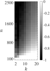
(a) CE

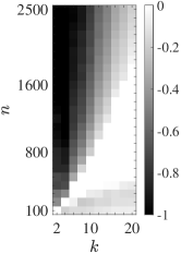
(b) LSPA (Ghosh et al., 2019)

Figure 4: Phase transition of estimation error in the noise case when $\sigma=0.1$ and $p=50$. The log base $10$ of the estimation error is plotted.

Aforementioned heuristic methods demonstrated satisfactory empirical performance on a few benchmark sets at tractable computational cost. However, these methods lack any statistical guarantees even under reasonable simplifying assumptions. The only exception is the LSPA algorithm, for which a rigorous analysis is recently provided by Ghosh et al. (2019). Under the standard Gaussian model for the data, Ghosh et al. (2019) provided a sample complexity for exact recovery of the parameter recovery starting from a good initialization. However, they observed a nontrivial gap between their sample complexity result and empirical behavior of the LSPA algorithm. Specifically, their sufficient condition for exact parameter recovery implies $n\gtrsim kp\pi_{\min}^{-3}\log(n/p)$, where $\pi_{\min}=\min_{j\in[k]}\mathbb{P}\{\bm{g}\in\mathcal{C}_{j}\}$ and $\bm{g}\sim\mathrm{Normal}(\bm{0},\bm{I}_{p})$. Their numerical results, however, illustrate that the empirical phase transition occurs at $n\approx kp\pi_{\min}^{-1}$ (see (Ghosh et al., 2019, Fig. 4)).

1.3 Contributions

We provide a scalable convex estimator for the max-linear regression problem that is formulated as a linear program and is backed by statistical guarantees. Under the standard Gaussian covariate model, the convex estimator (1.4) is guaranteed to recover the regression parameters exactly with high probability if the number of observations $n$ scales as $\pi_{\min}^{-4}p$ up to some logarithmic factors. This sample complexity implicitly depends on $k$ (i.e., the number of components) through $\pi_{\min}$. Particularly, when the $k$ linear components form a “well-balanced partition” in the sense that they are equally likely to achieve the maximum, the smallest probability $\pi_{\min}$ is close to $1/k$ and the derived sample complexity reduces to $k^{4}p$ up to the logarithmic factors.

2 Accuracy of the Convex Estimator

In this section, we provide our main results on the estimation error of the convex estimator in (1.4). We consider an anchor vector $\bm{\theta}$ constructed as

$$\bm{\theta}=\frac{1}{2n}\sum_{i=1}^{n}\nabla f_{i}(\widetilde{\bm{\beta}})\,$$ (2.1)

from a given initial estimate $\widetilde{\bm{\beta}}=[\widetilde{\bm{\beta}}_{1};\dots;\widetilde{\bm{\beta}}_{k}]\in\mathbb{R}^{kp}$.

The following theorem illustrates the sample complexity and the corresponding estimation error achieved by the estimator in (1.4). The estimation error is measured as the sum of the $\ell_{2}$ norms of the difference between the corresponding components of the ground truth $\bm{\beta}_{\star}$ and the estimate $\widehat{\bm{\beta}}$.

Theorem 1

Let $\{\widetilde{\mathcal{C}}_{j}\}_{j=1}^{k}$ be polyhedral cones defined similar to $\{\mathcal{C}_{j}\}_{j=1}^{k}$ in (1.6), with $\widetilde{\bm{\beta}}$ replacing $\bm{\beta}_{\star}$. With $\bm{\theta}$ given by (2.1) and $\{\bm{x}_{i}\}_{i=1}^{n}$ being i.i.d. $\mathrm{Normal}(\bm{0},\bm{I}_{p})$, suppose that $\widetilde{\bm{\beta}}$ is independent of $\{\bm{x}_{i}\}_{i=1}^{n}$. Then there exists a numerical constant $c>0$ such that if

$$\zeta\stackrel{{\scriptstyle\textup{\tiny def}}}{{=}}\min_{j\in[k]}\sqrt{\frac{\pi}{32}}\,\mathbb{P}^{2}\{\bm{g}\in{\mathcal{C}_{j}}\} -2\max_{j\in[k]}\sqrt{\mathbb{P}\{\bm{g}\in\widetilde{\mathcal{C}_{j}}\triangle{\mathcal{C}_{j}}\}}>0\,$$

and

$$n\geq c\,{\zeta}^{-2}\left(4p\log^{3}p\log^{5}k+4\log(\delta^{-1})\log k\right)\,,$$ (2.2)

then the solution $\widehat{\bm{\beta}}$ to the optimization problem in (1.4) obeys

$$\sum_{j=1}^{k}\|\bm{\beta}_{\star,j}-\widehat{\bm{\beta}}_{j}\|_{2}\leq\frac{2}{\zeta n}\sum_{i=1}^{n}|w_{i}|\,$$ (2.3)

with probability $1-\delta$.

3 Numerical results

We provide numerical results through Monte Carlo simulations for max-linear regression over generic data. The experiments were intended to illustrate two objectives: i) The lower bound on sufficient number of observations by Theorem 1 is consistent with empirical behavior of the convex estimator, and ii) The convex estimator provides competitive empirical performance to LSPA (Ghosh et al., 2019).

In the experiments, the convex estimator is implemented through the following equivalent linear program

$$\begin{array}[]{cl}\displaystyle\mathop{\mathrm{maximize}}_{(\bm{\beta}_{j})_{j=1}^{k},(t_{i})_{i=1}^{n}}&\displaystyle\langle{\bm{\theta}},[\bm{\beta}_{1};\dots;\bm{\beta}_{k}]\rangle\\ \mathrm{subject~{}to}&\displaystyle t_{i}\geq 0,~{}\langle\bm{x}_{i},\bm{\beta}_{j}\rangle-y_{i}\leq t_{i},~{}\frac{1}{n}\sum_{i=1}^{n}t_{i}\leq\eta,\quad\forall i\in[n],~{}\forall j\in[k]\,,\end{array}$$ (3.1)

where $\eta=\frac{1}{n}\sum_{i=1}^{n}(-w_{i})_{+}$ from (1.4). Since (3.1) is a standard linear program, it is highly scalable and can be solved by off-the-shelf-software packages such as CPLEX and Gurobi (Gurobi Optimization, 2021). For an extensive Monte Carlo simulation, we set the size of the regression problem to a moderate number so that the optimization can be solved efficiently using the Gurobi solver in MATLAB. The convex estimator is compared to the version of LSPA by Ghosh et al. (2019), which terminates the iterations once the maximum number of $200$ is reached.

To be compatible with the assumptions of Theorem 1, the regressors $\bm{x}_{1},\dots,\bm{x}_{n}$ are generated as i.i.d $\mathrm{Normal}(\bm{0},\bm{I}_{p})$. The ground truth regression parameter vector is normalized so that $\|\bm{\beta}_{\star}\|_{2}=1$. The entries of $\bm{\beta}_{\star}$ are chosen so that they correspond to a well-balanced case. Specifically, in the first set of simulations (Figures 1, 2, 3 and 4), $\bm{\beta}_{\star,1},\dots,\bm{\beta}_{\star,k}$ are set to be $p$-dimensional standard basis vectors. In the second set (Figure 5), $\bm{\beta}_{\star,1},\dots,\bm{\beta}_{\star,k}$ are generated i.i.d. $\mathrm{Normal}(\bm{0},\bm{I}_{kp})$. In all of the experiments, the given initial estimate $\widetilde{\bm{\beta}}$ is a slight perturbation of $\bm{\beta}_{\star}$ in the sense that $\widetilde{\bm{\beta}}=\bm{\beta}_{\star}+\bm{\epsilon}$, where $\bm{\epsilon}\sim\mathrm{Normal}(\bm{0},1/(1000kp)\bm{I}_{kp})$. Since the initial estimate $\widetilde{\bm{\beta}}$ is a slightly perturbed version of the ground truth $\bm{\beta}_{\star}$, we expect the assumption on $\zeta$ in Theorem 1 to hold. We measure the normalized estimation error as the median of normalized estimation errors $\sum_{j=1}^{k}\|\widehat{\bm{\beta}}_{j}-\bm{\beta}_{\star,j}\|_{2}/\sum_{j=1}^{k}\|\bm{\beta}_{\star,j}\|_{2}$ over $50$ trials.

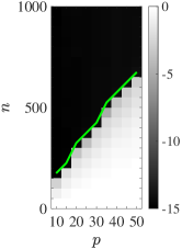
(a) CE

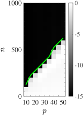
(b) LSPA (Ghosh et al., 2019)

Figure 1: Phase transition of estimation error in the noiseless case for $k=10$. The log base $10$ of the estimation error is plotted. Above the green line denotes the regime for exact recovery with error below $10^{-5}$.

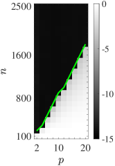
(a) CE

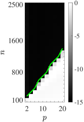
(b) LSPA (Ghosh et al., 2019)

Figure 2: Phase transition of estimation error in the noiseless case for $p=50$. The log base $10$ of the estimation error is plotted. Above the green line denotes the regime for exact recovery with error below $10^{-5}$.

Figures 1 and 2 illustrate the normalized estimation error in the noiseless scenario, as a function of the sample size, $n$, as well as the dimension and the number of segments of the parameter, $p$ and $k$. Green lines in these figures represent where the phase transition occurs in the sense that the median of normalized estimation errors falls below $10^{-5}$. In Figure 1, the number of segments, $k$, is fixed to $10$. Figure 1 suggests that the successful recovery occurs if $n$ grows linearly with $p$, for both CE and LSPA in a similar way. A complementary view is provided by Figure 2, corresponding to a varying number of segment $k$, and a fixed dimension of $p=50$. As Ghosh et al. (2019) pointed out, their sufficient condition for exact recovery is conservative compared to the observed empirical performance of LSPA. To be specific, the sample complexity of LSPA in their numerical results depends on $k$ instead of $k^{4}$. We observed a similar gap between the theoretical prediction in Theorem 1 and the empirical performance. That is, the phase transition of CE in 2 occurs when $n$ is proportional to $k$ instead of ${k^{2}}$. In fact, as Figures 1 and 2 suggest, the sample complexity of successful recovery using LSPA is only a constant factor better than CE in the noiseless scenario.

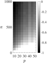
(a) CE

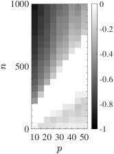
(b) LSPA (Ghosh et al., 2019)

Figure 3: Phase transition of estimation error in the noise case when $\sigma=0.1$ and $k=10$. The log base $10$ of the estimation error is plotted.

Figures 3 and 4 are the analogs of Figures 1 and 2 for noisy measurements. The noise standard deviation $\sigma$ is set to $0.1$. Figures 3 and 4 suggest that in the noisy scenario, as the number of observations required by the LSPA for accurate recovery, compared to CE, grows more rapidly as $k$ or $p$ increase. This behavior is in contrast with comparable performance of the two algorithms in the noiseless setting. Figures 3(b) and 4(b) contain peculiar triangular regions adjacent to the horizontal axis where a nontrivial normalized error is achieved. We believe that these regions are the artifact of the LSPA algorithm being stuck around the initialization, which is close to the ground truth parameter, for small $n$.

	$\sigma=0.05$	$\sigma=0.1$	$\sigma=0.15$
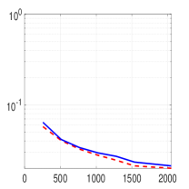
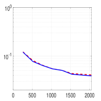
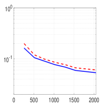
	$\sigma=0.2$	$\sigma=0.25$	$\sigma=0.3$

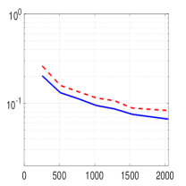
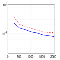
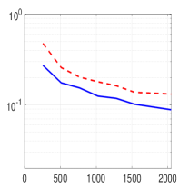
Figure 5: Log-scale of $\|\bm{\beta}_{\star}-\widehat{\bm{\beta}}\|_{1,2}/{\left\lVert\bm{\beta}_{\star}\right\rVert}_{1,2}$ versus the number of observations $n$ for CE (solid line) and LSPA (dotted line) according to $\sigma$ when $k=5$ and $p=10$. The estimation error is calculated as the median of $50$ trials.

Figure 5 shows log-scale plot of the normalized estimation error for both the CE and LSPA with respect to the number of observations $n$ at fixed $k=5$ and $p=10$. Note that while LSPA has an asymptotically vanishing error (i.e., it is consistent) (Ghosh et al., 2019), CE appears to be a biased estimator whose bias depends on the noise strength in (2.3). Despite this drawback, Figure 5 shows that CE outperforms LSPA for a moderate number of observations. This implies that CE is more practical estimator in that we want to estimate parameters with the limited number of samples in practice. Furthermore, we can observe that the required oversampling factor of LSPA is more sensitive to $\sigma$, compared to CE, in the sense that LSPA requires more observations than CE for accurate estimation as $\sigma$ increases.

4 Proof of Theorem 1

We prove Theorem 1 in two steps. First, in the following proposition, we present a sufficient condition for robust estimation by convex program in (1.4). Then we derive an upper bound on $\varrho$ in the proposition, which provides the sample complexity condition along with the corresponding error bound in Theorem 1.

Proposition 1

Under the hypothesis of Theorem 1, suppose that $\widetilde{\bm{\beta}}$ satisfies

$$\varrho\stackrel{{\scriptstyle\textup{\tiny def}}}{{=}}\inf_{\begin{subarray}{l}j\in[k]\\ \bm{w}\in\mathbb{S}^{p-1}\end{subarray}}\mathbb{E}\,\mathbb{1}_{\mathcal{C}_{j}}(\bm{g})\left|\left\langle\bm{g},\bm{w}\right\rangle\right|-\sup_{\begin{subarray}{l}j\in[k]\\ \bm{w}\in\mathbb{S}^{p-1}\end{subarray}}\mathbb{E}\mathbb{1}_{\widetilde{\mathcal{C}}_{j}\setminus\mathcal{C}_{j}}(\bm{g})\langle\bm{g},\bm{w}\rangle_{+}-\sup_{\begin{subarray}{l}j\in[k]\\ \bm{w}\in\mathbb{S}^{p-1}\end{subarray}}\mathbb{E}\mathbb{1}_{\mathcal{C}_{j}\setminus\widetilde{\mathcal{C}}_{j}}(\bm{g})\langle\bm{g},\bm{w}\rangle_{+}>0\,.$$ (4.1)

Then there exists a numerical constant $c>0$ such that if

$$n\geq c\varrho^{-2}\left(4p\log^{3}p\log^{5}k+4\log(\delta^{-1})\log k\right)\,,$$ (4.2)

then the solution $\widehat{\bm{\beta}}$ to the optimization problem in (1.4) obeys

$$\sum_{j=1}^{k}\|\bm{\beta}_{\star,j}-\widehat{\bm{\beta}}_{j}\|_{2}\leq\frac{2}{\varrho n}\sum_{i=1}^{n}|w_{i}|$$ (4.3)

with probability $1-\delta$.

Proof  We first show that, for a sufficiently large $\rho>0$, the following three conditions cannot hold simultaneously:

$$\frac{1}{n}\sum_{i=1}^{n}\left(f_{i}(\bm{\beta}_{\star}+\bm{z})-y_{i}\right)_{+}\leq\eta\,,$$ (4.4)

$${\left\lVert\bm{z}\right\rVert}_{1,2}>\rho\,,$$ (4.5)

$$\langle\bm{\theta},\bm{z}\rangle\geq 0\,.$$ (4.6)

Therefore, assuming (4.5) and (4.6) hold, it suffices to show

$$\mathcal{L}(\bm{z})\stackrel{{\scriptstyle\textup{\tiny def}}}{{=}}\frac{1}{n}\sum_{i=1}^{n}\left(f_{i}(\bm{\beta}_{\star}+\bm{z})-y_{i}\right)_{+}>\eta\,.$$ (4.7)

To this end, we derive a lower bound on $\mathcal{L}(\bm{z})$ as follows:

$$\mathcal{L}(\bm{z}) \geq\frac{1}{n}\sum_{i=1}^{n}\left(f_{i}(\bm{\beta}_{\star}+\bm{z})-f_{i}(\bm{\beta}_{\star})\right)_{+}-\frac{1}{n}\sum_{i=1}^{n}(w_{i})_{+}$$

$$\overset{\mathrm{(a)}}{\geq}\frac{1}{n}\sum_{i=1}^{n}\left(\left\langle\nabla f_{i}(\bm{\beta}_{\star}),\bm{z}\right\rangle\right)_{+}-\frac{1}{n}\sum_{i=1}^{n}(w_{i})_{+}$$

$$=\frac{1}{n}\sum_{i=1}^{n}\frac{\left|\left\langle\nabla f_{i}(\bm{\beta}_{\star}),\bm{z}\right\rangle\right|}{2}+\frac{1}{n}\sum_{i=1}^{n}\frac{\left\langle\nabla f_{i}(\bm{\beta}_{\star}),\bm{z}\right\rangle}{2}-\frac{1}{n}\sum_{i=1}^{n}(w_{i})_{+}$$

$$=\frac{1}{n}\sum_{i=1}^{n}\frac{\left|\left\langle\nabla f_{i}(\bm{\beta}_{\star}),\bm{z}\right\rangle\right|}{2}+\frac{1}{n}\sum_{i=1}^{n}\frac{\left\langle\nabla f_{i}(\bm{\beta}_{\star}),\bm{z}\right\rangle}{2}-\langle\bm{\theta},\bm{z}\rangle+\langle\bm{\theta},\bm{z}\rangle-\frac{1}{n}\sum_{i=1}^{n}(w_{i})_{+}$$

$$\overset{\mathrm{(b)}}{=}\langle\bm{\theta},\bm{z}\rangle-\frac{1}{n}\sum_{i=1}^{n}(w_{i})_{+}+\frac{1}{n}\sum_{i=1}^{n}\frac{\left|\left\langle\nabla f_{i}(\bm{\beta}_{\star}),\bm{z}\right\rangle\right|}{2}+\frac{1}{n}\sum_{i=1}^{n}\frac{\langle\nabla f_{i}(\bm{\beta}_{\star})-\nabla f_{i}(\widetilde{\bm{\beta}}),\bm{z}\rangle}{2}$$

$$\overset{\mathrm{(c)}}{=}\langle\bm{\theta},\bm{z}\rangle-\frac{1}{n}\sum_{i=1}^{n}(w_{i})_{+}+\frac{1}{n}\sum_{i=1}^{n}\sum_{j=1}^{k}\frac{\mathbb{1}_{\mathcal{C}_{j}}(\bm{x}_{i})|\langle\bm{x}_{i},\bm{z}_{j}\rangle|}{2}+\frac{1}{n}\sum_{i=1}^{n}\sum_{j=1}^{k}\frac{\{\mathbb{1}_{\mathcal{C}_{j}}(\bm{x}_{i})-\mathbb{1}_{\widetilde{\mathcal{C}}_{j}}(\bm{x}_{i})\}\langle\bm{x}_{i},\bm{z}_{j}\rangle}{2}\,,$$ (4.8)

where (a) holds by the convexity of $f_{i}$, which implies

$$f_{i}(\bm{\beta}_{\star}+\bm{z})\geq f_{i}(\bm{\beta}_{\star})+\langle\nabla{f_{i}(\bm{\beta}_{\star})},\bm{z}\rangle\,,$$

(b) follows from (2.1), and (c) is obtained by calculating $\nabla f_{i}(\bm{\beta})$ at $\bm{\beta}=\bm{\beta}_{\star}$ and $\bm{\beta}=\widetilde{\bm{\beta}}$. We further proceed by obtaining lower bounds on the last two terms in (4.8) by the following lemmas, which are proved in Appendices A.1 and A.2.

Lemma 1

Let $(V_{\bm{z}})_{\bm{z}\in\mathbb{R}^{kp}}$ be a random process defined by

$$V_{\bm{z}}\stackrel{{\scriptstyle\textup{\tiny def}}}{{=}}\frac{1}{n}\sum_{i=1}^{n}\sum_{j=1}^{k}\mathbb{1}_{\mathcal{C}_{j}}(\bm{x}_{i})\left|\langle\bm{x}_{i},\bm{z}_{j}\rangle\right|\,,$$

where $\bm{x}_{1},\dots,\bm{x}_{n}$ are i.i.d. $\mathrm{Normal}(\bm{0},\bm{I}_{p})$. Then, for $\bm{g}\sim\mathrm{Normal}(\bm{0},\bm{I}_{p})$ and any $\delta\in(0,1)$, there exists a numerical constant $c_{1}>0$ such that

$$\underline{V}\stackrel{{\scriptstyle\textup{\tiny def}}}{{=}}\inf_{{\left\lVert\bm{z}\right\rVert}_{1,2}=1}V_{\bm{z}}\geq\min_{j\in[k],\bm{w}\in\mathbb{S}^{p-1}}\mathbb{E}\,\mathbb{1}_{\mathcal{C}_{j}}(\bm{g})\left|\left\langle\bm{g},\bm{w}\right\rangle\right|-c_{1}\left(\frac{p\log^{3}p\log^{5}k+\log(\delta^{-1})\log k}{n}\right)^{1/2}\,$$

holds with probability at least $1-\delta/2$.

Lemma 2

Let $(Q_{\bm{z}})_{\bm{z}\in B_{1,2}}$ be a random process defined by

$$Q_{\bm{z}}\stackrel{{\scriptstyle\textup{\tiny def}}}{{=}}\frac{1}{n}\sum_{i=1}^{n}\sum_{j=1}^{k}\left\{\mathbb{1}_{\widetilde{\mathcal{C}}_{j}}(\bm{x}_{i})-\mathbb{1}_{\mathcal{C}_{j}}(\bm{x}_{i})\right\}\langle\bm{x}_{i},\bm{z}_{j}\rangle\,,$$

where $\bm{x}_{1},\dots,\bm{x}_{n}$ are i.i.d. $\mathrm{Normal}(\bm{0},\bm{I}_{p})$. Then, for $\bm{g}\sim\mathrm{Normal}(\bm{0},\bm{I}_{p})$ and any $\delta\in(0,1)$, there exists a numerical constant $c_{2}>0$ such that

$$\overline{Q}\stackrel{{\scriptstyle\textup{\tiny def}}}{{=}}\sup_{{\left\lVert\bm{z}\right\rVert}_{1,2}=1}Q_{\bm{z}}\leq \max_{j\in[k],\bm{w}\in\mathbb{S}^{p-1}}\mathbb{E}\mathbb{1}_{\widetilde{\mathcal{C}}_{j}\setminus\mathcal{C}_{j}}(\bm{g})\langle\bm{g},\bm{w}\rangle_{+}+\max_{j\in[k],\bm{w}\in\mathbb{S}^{p-1}}\mathbb{E}\mathbb{1}_{\mathcal{C}_{j}\setminus\widetilde{\mathcal{C}}_{j}}(\bm{g})\langle\bm{g},\bm{w}\rangle_{+}$$

$$+c_{2}\left(\frac{p\log^{3}p\log^{5}k+\log(\delta^{-1})\log k}{n}\right)^{1/2}\,$$

holds with probability at least $1-\delta/2$.

Since $V_{\bm{z}}$ are $Q_{\bm{z}}$ are homogeneous in $\bm{z}$, we obtain that the third term in the right-hand side of (4.8) is written as $V_{\bm{z}}$ and lower-bounded by

$$\frac{V_{\bm{z}}}{2}\geq\frac{\underline{V}{\left\lVert\bm{z}\right\rVert}_{1,2}}{2}\,.$$ (4.9)

Similarly, the last term in the right-hand side of (4.8) is written as $-Q_{\bm{z}}$ and lower-bounded by

$$-\frac{Q_{\bm{z}}}{2}\geq-\frac{\overline{Q}{\left\lVert\bm{z}\right\rVert}_{1,2}}{2}\,.$$ (4.10)

Furthermore, by Lemmas 1 and 2, the condition in (4.2) implies that

$$\underline{V}-\overline{Q}\geq\varrho>0$$ (4.11)

holds with probability $1-\delta$. Then we choose $\rho$ so that it satisfies

$$\rho=\frac{2}{\underline{V}-\overline{Q}}\cdot\frac{1}{n}\sum_{i=1}^{n}|w_{i}|\,.$$

Next, by plugging in the above estimates to (4.8), we obtain that, under the event in (4.11), the conditions in (4.5) and (4.6) imply

$$\mathcal{L}(\bm{z}) \geq\langle\bm{\theta},\bm{z}\rangle-\frac{1}{n}\sum_{i=1}^{n}(w_{i})_{+}+\frac{(\underline{V}-\overline{Q}){\left\lVert\bm{z}\right\rVert}_{1,2}}{2}$$

$$>-\frac{1}{n}\sum_{i=1}^{n}(w_{i})_{+}+\frac{(\underline{V}-\overline{Q})\rho}{2}$$

$$=-\frac{1}{n}\sum_{i=1}^{n}(w_{i})_{+}+\frac{1}{n}\sum_{i=1}^{n}|w_{i}|$$

$$=\frac{1}{n}\sum_{i=1}^{n}(-w_{i})_{+}=\eta\,.$$

This lower bound implies (4.7). Therefore we have shown that the three conditions in (4.4), (4.5), and (4.6) cannot hold simultaneously. It remains to apply the claim to a special case.

Let $\widehat{\bm{z}}=\widehat{\bm{\beta}}-\bm{\beta}_{\star}$. Recall that both $\widehat{\bm{\beta}}$ and $\bm{\beta}_{\star}$ are feasible for the optimization problem in (1.4). Moreover, since $\widehat{\bm{\beta}}$ is the maximizer, it follows that $\langle\bm{\theta},\widehat{\bm{\beta}}\rangle\geq\langle\bm{\theta},\bm{\beta}_{\star}\rangle$, which implies $\langle\bm{\theta},\widehat{\bm{z}}\rangle\geq 0$. Therefore the conditions in (4.4) and (4.6) are satisfied with $\bm{z}$ substituted by $\widehat{\bm{z}}$. Since the three conditions cannot be satisfied simultaneously, the condition in (4.5) cannot hold, i.e. $\widehat{\bm{z}}$ satisfies

$${\left\lVert\widehat{\bm{z}}\right\rVert}_{1,2}\leq\rho\leq\frac{2}{\varrho n}\sum_{i=1}^{n}|w_{i}|\,.$$

Thus we obtain the desired assertion.  

Next we use the following lemma to obtain a lower bound on $\varrho$ in (4.1).

Lemma 3

Let $\mathcal{A}\subset\mathbb{R}^{p}$ be of finite Gaussian measure and $\bm{g}\sim\mathrm{Normal}(\bm{0},\bm{I}_{p})$. Then we have

$$\inf_{\begin{subarray}{l}\bm{w}\in\mathbb{S}^{p-1}\end{subarray}}\mathbb{E}\,\mathbb{1}_{\mathcal{A}}(\bm{g})\left|\left\langle\bm{g},\bm{w}\right\rangle\right|\geq\sqrt{\frac{\pi}{32}}\,\mathbb{P}^{2}\{\bm{g}\in{\mathcal{A}}\}\,$$

and

$$\sup_{\begin{subarray}{l}\bm{w}\in\mathbb{S}^{p-1}\end{subarray}}\mathbb{E}\mathbb{1}_{\mathcal{A}}(\bm{g})\langle\bm{g},\bm{w}\rangle_{+}\leq\sqrt{\mathbb{P}\{\bm{g}\in\mathcal{A}\}}\,.$$

Proof  For an arbitrarily fixed $\epsilon>0$, let $S_{\epsilon}\subset\mathbb{R}^{p}$ denote the set defined by

$$S_{\epsilon}:=\{\bm{x}\in\mathbb{R}^{p}:|\langle\bm{x},\bm{w}\rangle|<\epsilon\}\,.$$

Then we have

$$\mathbb{E}\mathbb{1}_{\mathcal{C}}(\bm{g})|{\langle\bm{g},\bm{w}\rangle}| \geq\epsilon\,\mathbb{E}\mathbb{1}_{\mathcal{C}}(\bm{g})\mathbb{1}_{\mathcal{S}_{\epsilon}^{\mathrm{c}}}(\bm{g})$$

$$=\epsilon\,\mathbb{E}\left(\mathbb{1}_{\mathcal{C}}(\bm{g})-\mathbb{1}_{\mathcal{C}}(\bm{g})\mathbb{1}_{\mathcal{S}_{\epsilon}}(\bm{g})\right)$$

$$\geq\epsilon\,\mathbb{E}\left(\mathbb{1}_{\mathcal{C}}(\bm{g})-\mathbb{1}_{\mathcal{S}_{\epsilon}}(\bm{g})\right)$$

$$=\epsilon\,\left(\mathbb{P}\{\bm{g}\in\mathcal{C}\}-\mathbb{P}\{\bm{g}\in\mathcal{S}_{\epsilon}\}\right)\,.$$ (4.12)

Moreover, since $\langle\bm{g},\bm{w}\rangle\sim\mathrm{Normal}(0,1)$, $\mathbb{P}\{\bm{g}\in S_{\epsilon}\}$ is upper-bounded by

$$\mathbb{P}\{\bm{g}\in S_{\epsilon}\} =\mathbb{P}\{|\langle\bm{g},\bm{w}\rangle|<\epsilon\}=\int_{-\epsilon}^{\epsilon}\frac{1}{\sqrt{2\pi}}e^{-u^{2}/2}du\leq\delta\sqrt{\frac{2}{\pi}}\,.$$ (4.13)

By plugging in (4.13) to (4.12), we obtain

$$\mathbb{E}\mathbb{1}_{\mathcal{C}}(\bm{g})|{\langle\bm{g},\bm{w}\rangle}|\geq\epsilon\left(\mathbb{P}\{\bm{g}\in\mathcal{C}\}-\epsilon\sqrt{\frac{2}{\pi}}\right)\,.$$ (4.14)

Since the parameter $\epsilon>0$ was arbitrary, one can we maximize the right-hand side of (4.14) with respect to $\epsilon$ to obtain the tightest lower bound. Note that the objective is a concave quadratic function and the maximum is attained at $\epsilon=\sqrt{{\pi}/{8}}\,\mathbb{P}\left\{\bm{g}\in\mathcal{C}\right\}$. This provides the lower bound in the first assertion. Next, by the Cauchy-Schwarz inequality, we obtain the upper bound in the second assertion as follows:

$$\mathbb{E}\mathbb{1}_{\mathcal{A}}(\bm{g})\langle\bm{g},\bm{w}\rangle_{+}\leq\sqrt{\mathbb{E}\left(\mathbb{1}_{\mathcal{A}}(\bm{g})\right)^{2}}\sqrt{\mathbb{E}{\langle\bm{g},\bm{w}\rangle_{+}^{2}}}=\sqrt{\mathbb{E}\mathbb{1}_{\mathcal{A}}(\bm{g})}\sqrt{\frac{\mathbb{E}{\langle\bm{g},\bm{w}\rangle^{2}}}{2}}=\sqrt{\frac{\mathbb{P}\{\bm{g}\in\mathcal{A}\}}{2}}\,.$$

 

Finally, by applying Lemma 3 to each of the expectation terms in $\varrho$, we obtain a lower bound on $\varrho$ given by

$$\varrho \geq\min_{j\in[k]}\sqrt{\frac{\pi}{32}}\,\mathbb{P}^{2}\left\{\bm{g}\in\mathcal{C}_{j}\right\}-\max_{j\in[k]}\sqrt{\mathbb{P}\left\{\bm{g}\in{\mathcal{C}_{j}}\setminus\widetilde{\mathcal{C}_{j}}\right\}}-\max_{j\in[k]}\sqrt{\mathbb{P}\{\bm{g}\in\widetilde{\mathcal{C}_{j}}\setminus\mathcal{C}_{j}\}}\,$$

$$\geq\min_{j\in[k]}\sqrt{\frac{\pi}{32}}\,\mathbb{P}^{2}\left\{\bm{g}\in\mathcal{C}_{j}\right\}-2\max_{j\in[k]}\sqrt{\mathbb{P}\left\{\bm{g}\in{\mathcal{C}_{j}}\triangle\widetilde{\mathcal{C}_{j}}\right\}}\,,$$ (4.15)

where the second inequality holds since $\widetilde{\mathcal{C}_{j}}\triangle{\mathcal{C}_{j}}=(\widetilde{\mathcal{C}_{j}}\setminus\mathcal{C}_{j})\cup(\mathcal{C}_{j}\setminus\widetilde{\mathcal{C}_{j}})$ for all $j\in[k]$. This implies that (2.2) is a sufficient condition for (4.2). Moreover, substituting $\varrho$ in (4.3) by the lower bound in (4.15) provides (2.3). This completes the proof of Theorem 1.

5 Discussion on Tightness of Theorem 1

The sample complexity in Theorem 1 is tight given an accurate initial estimate. This can be deduced from the following example, where the lower bound on $\varrho$ by Lemma 3 is tight in terms of its dependence on $\mathbb{P}\left\{\bm{g}\in\mathcal{C}_{j}\right\}$ for $j\in[k]$.

Example 1

Let $p=2$. Then $\widetilde{\mathcal{C}}_{j}\setminus\mathcal{C}_{j}$ and $\mathcal{C}_{j}\setminus\widetilde{\mathcal{C}}_{j}$ are Lorentz cones. Let $\theta_{\mathcal{C}_{j}}$, $\theta_{\mathcal{C}_{j}\setminus\widetilde{\mathcal{C}_{j}}}$ and ${\theta_{\widetilde{\mathcal{C}_{j}}\setminus{{\mathcal{C}_{j}}}}}$ denote the angular width of $\mathcal{C}_{j}$, ${\mathcal{C}}_{j}\setminus\widetilde{\mathcal{C}_{j}}$, and $\widetilde{\mathcal{C}_{j}}\setminus{\mathcal{C}}_{j}$ respectively. Furthermore, we assume that

$$\min_{j\in[k]}\mathbb{P}\left\{\bm{g}\in\mathcal{C}_{j}\right\}\geq\max_{j\in[k]}\mathbb{P}\left\{\bm{g}\in{\mathcal{C}_{j}}\triangle\widetilde{\mathcal{C}_{j}}\right\}\,.$$ (5.1)

In this case, the parameter $\varrho$ in Proposition 1 is expressed as

$$\varrho=\frac{\sqrt{2}\Gamma(3/2)}{\Gamma(1)}\left[\min_{j\in[k]}\frac{2}{\pi}\sin^{2}\left(\frac{\theta_{\mathcal{C}_{j}}}{4}\right)-\max_{j\in[k]}\frac{1}{\pi}\sin\left({\frac{\theta_{\widetilde{\mathcal{C}_{j}}\setminus{\mathcal{C}_{j}}}}{2}}\right)-\max_{j\in[k]}\frac{1}{\pi}\sin\left({\frac{\theta_{\mathcal{C}_{j}\setminus\widetilde{\mathcal{C}_{j}}}}{2}}\right)\right]\,.$$ (5.2)

When $\theta_{\mathcal{C}}$ is small enough, $\sin(\theta_{\mathcal{C}})\approx{\theta_{\mathcal{C}}}$ holds by the Taylor series approximation. Hence, there exists numerical constants $c_{1}>0$ and $c_{2}>0$ such that

$$\varrho=c_{1}\min_{j\in[k]}{\mathbb{P}^{2}\{\bm{g}\in\mathcal{C}_{j}\}}-c_{2}\max_{j\in[k]}\mathbb{P}\{\bm{g}\in\widetilde{\mathcal{C}_{j}}\triangle{\mathcal{C}_{j}}\}\,.$$

This example shows that $\zeta$ in Theorem 1 is tight in the sense that the dominating term in both $\varrho$ and $\zeta$ is proportional to the squared probability measure of the smallest $\mathcal{C}_{j}$.

Let $\theta_{\mathcal{C}_{j}}$ denote the angular width of $\mathcal{C}_{j}$. Without loss of generality, we may assume that $\min_{j\in[k]}\theta_{\mathcal{C}_{j}}\leq\pi$. Furthermore, the assumption in (5.1) implies that the angular width of $\mathcal{C}_{j}\triangle\widetilde{\mathcal{C}}_{j}$ is at most $\pi$ for all $j\in[k]$. Therefore, the identity in (5.2) is obtained by applying the following lemma, proved in Appendix A.3, to the infimum/supremum of expectation terms in (4.1).

Lemma 4

Let $\mathcal{C}$ be a polyhedral cone in $\mathbb{R}^{2}$ and $\bm{g}\sim\mathrm{Normal}(\bm{0},\bm{I}_{2})$. Suppose that the angular width of $\mathcal{C}$, denoted by $\theta_{\mathcal{C}}$ satisfies $0\leq\theta_{\mathcal{C}}\leq\pi$. Then we have

$$\inf_{\begin{subarray}{l}\bm{w}\in\mathbb{S}^{1}\end{subarray}}\mathbb{E}\,\mathbb{1}_{\mathcal{C}}(\bm{g})\left|\left\langle\bm{g},\bm{w}\right\rangle\right|=\frac{2\sqrt{2}\Gamma({3}/{2})}{\pi\Gamma(2)}\sin^{2}\left(\frac{\theta_{\mathcal{C}}}{4}\right)\,$$

and

$$\sup_{\begin{subarray}{l}\bm{w}\in\mathbb{S}^{1}\end{subarray}}\mathbb{E}\mathbb{1}_{{\mathcal{C}}}(\bm{g})\langle\bm{g},\bm{w}\rangle_{+}=\frac{\sqrt{2}\Gamma({3}/{2})}{\pi\Gamma(2)}\sin\left({\frac{{\theta_{\mathcal{C}}}}{2}}\right)\,.$$

6 Discussion

As discussed in Section 3, the proposed convex estimator has weakness in the sense that it does not provide a consistent estimator in the asymptotic in the number of observations. To relax this weakness, one might consider an alternative optimization that has the data fidelity term as a penalty instead of a constraint. The analysis of this alternative convex estimator will be investigated in our future work. Also, we will investigate the effect of nontrivial offset terms in the max-affine case. We conjecture that it might be necessary to introduce a different stochastic model on regressors than the standard Gaussian model to avoid degenerate partition by the max-affine model.

A Proof of Supporting Lemmas

A.1 Proof of Lemma 1

For any $\bm{z}$ satisfying ${\left\lVert\bm{z}\right\rVert}_{1,2}=1$, we have

$$V_{\bm{z}}\geq\min_{{\left\lVert\bm{z}\right\rVert}_{1,2}=1}\mathbb{E}V_{\bm{z}}-\sup_{\bm{z}\in B_{1,2}}|V_{\bm{z}}-\mathbb{E}V_{\bm{z}}|\,.$$ (A.1)

In what follows, we derive lower estimates of the summands in the right-hand side of (A.1).

First, we derive a lower bound on $\min_{{\left\lVert\bm{z}\right\rVert}_{1,2}=1}\mathbb{E}V_{\bm{z}}$. Since $\bm{x}_{1},\dots,\bm{x}_{n}$ are i.i.d. $\mathrm{Normal}(\bm{0},\bm{I}_{p})$, we have

$$\mathbb{E}V_{\bm{z}}=\mathbb{E}\,\frac{1}{n}\sum_{i=1}^{n}\sum_{j=1}^{k}\mathbb{1}_{\mathcal{C}_{j}}(\bm{x}_{i})\left|\langle\bm{x}_{i},\bm{z}_{j}\rangle\right|=\mathbb{E}\,\sum_{j=1}^{k}\mathbb{1}_{\mathcal{C}_{j}}(\bm{g})\left|\langle\bm{g},\bm{z}_{j}\rangle\right|=\sum_{j=1}^{k}{\left\lVert\bm{z}_{j}\right\rVert}_{2}\mathbb{E}\,\mathbb{1}_{\mathcal{C}_{j}}(\bm{g})\left|\left\langle\bm{g},\frac{\bm{z}_{j}}{{\left\lVert\bm{z}_{j}\right\rVert}_{2}}\right\rangle\right|\,,$$

where $\bm{z}=[\bm{z}_{1};\ \dots;\ \bm{z}_{k}]$. Then $\mathbb{E}V_{\bm{z}}$ is lower-bounded by

$$\mathbb{E}V_{\bm{z}}\geq{\left\lVert\bm{z}\right\rVert}_{1,2}\inf_{j\in[k],\bm{w}\in\mathbb{S}^{p-1}}\mathbb{E}\,\mathbb{1}_{\mathcal{C}_{j}}(\bm{g})\left|\left\langle\bm{g},\bm{w}\right\rangle\right|\,.$$

Next, we show that $(V_{\bm{z}}-\mathbb{E}V_{\bm{z}})_{\bm{z}\in B_{1,2}}$ is concentrated around $0$ with high probability by using the following lemma.

Lemma 5

Suppose that $\mathcal{A}_{1},\dots,\mathcal{A}_{k}$ be disjoint subsets in $\mathbb{R}^{p}$. Let $(U_{\bm{z}})_{\bm{z}\in B_{1,2}}$ be a random process defined by

$$U_{\bm{z}}\stackrel{{\scriptstyle\textup{\tiny def}}}{{=}}\frac{1}{n}\sum_{i=1}^{n}\sum_{j=1}^{k}\mathbb{1}_{\mathcal{A}_{j}}(\bm{x}_{i})\langle\bm{x}_{i},\bm{z}_{j}\rangle_{+}\,,$$ (A.2)

where $\bm{x}_{1},\dots,\bm{x}_{n}$ are i.i.d. $\mathrm{Normal}(\bm{0},\bm{I}_{p})$. Then, for any $\delta\in(0,1)$, there exists a numerical constant $c>0$ such that

$$\sup_{\bm{z}\in B_{1,2}}\left|U_{\bm{z}}-\mathbb{E}U_{\bm{z}}\right|\leq c\left(\frac{p\log^{3}p\log^{5}k+\log(\delta^{-1})\log k}{n}\right)^{1/2}\,$$ (A.3)

holds with probability at least $1-\delta$.

Proof  We first show that $U_{\bm{z}}$ has subgaussian increments with respect to the $\ell_{\infty}^{k}(\ell_{2}^{p})$-norm, i.e.

$${\left\lVert U_{\bm{z}}-U_{\bm{z}^{\prime}}\right\rVert}_{\psi_{2}}\lesssim\frac{\sqrt{\log k}}{\sqrt{n}}\,{\left\lVert\left(\bm{z}_{j}\right)_{j=1}^{k}-\left(\bm{z}^{\prime}_{j}\right)_{j=1}^{k}\right\rVert}_{\ell_{\infty}^{k}(\ell_{2}^{p})}\,.$$ (A.4)

Since $\mathcal{A}_{1},\dots,\mathcal{A}_{k}$ are disjoint, it follows that

$$\left|{U_{\bm{z}}-U_{\bm{z}^{\prime}}}\right|\leq\frac{1}{n}\sum_{i=1}^{n}\sum_{j=1}^{k}\mathbb{1}_{\mathcal{A}_{j}}(\bm{x}_{i})\left|\langle\bm{x}_{i},\bm{z}_{j}-\bm{z}_{j}^{\prime}\rangle\right|\leq\frac{1}{n}\sum_{i=1}^{n}\max_{1\leq{j}\leq{k}}\left|\langle\bm{x}_{i},\bm{z}_{j}-\bm{z}_{j}^{\prime}\rangle\right|\,\,$$ (A.5)

holds almost surely, where the last step follows from Hölder’s inequality. We proceed with the following lemma.

Lemma 6 (van der Vaart and Wellner (1996, Lemma 2.2.2))

Let $\bm{g}\sim\mathrm{Normal}(\bm{0},\bm{I}_{p})$ and $\bm{a}_{1},\dots,\bm{a}_{k}\in\mathbb{R}^{p}$. Then

$${\left\lVert\max_{j\in[k]}\left|\langle\bm{g},\bm{a}_{j}\rangle\right|\right\rVert}_{\psi_{2}}\lesssim\sqrt{\log k}\max_{j\in[k]}{\left\lVert\bm{a}_{j}\right\rVert}_{2}\,.$$

It follows from (A.5) and Lemma 6 that

$${\left\lVert U_{\bm{z}}-U_{\bm{z}^{\prime}}\right\rVert}_{\psi_{2}} \leq{\left\lVert\frac{1}{n}\sum_{i=1}^{n}\max_{j\in[k]}\left|{\langle{\bm{x}_{i},\bm{z}_{j}-\bm{z}_{j}^{\prime}}\rangle}\right|\right\rVert}_{\psi_{2}}$$

$$\lesssim\frac{1}{n}\sqrt{\sum_{i=1}^{n}{\left\lVert\max_{j\in[k]}\left|{\langle{\bm{x}_{i},\bm{z}_{j}-\bm{z}_{j}^{\prime}}\rangle}\right|\right\rVert}_{\psi_{2}}^{2}}$$

$$\lesssim\frac{\sqrt{\log k}}{\sqrt{n}}\max_{j\in[k]}{\left\lVert\bm{z}_{j}-\bm{z}^{\prime}_{j}\right\rVert}_{2}$$

$$=\frac{\sqrt{\log k}}{\sqrt{n}}\,{\left\lVert\left(\bm{z}_{j}\right)_{j=1}^{k}-\left(\bm{z}^{\prime}_{j}\right)_{j=1}^{k}\right\rVert}_{\ell_{\infty}^{k}(\ell_{2}^{p})}\,,$$

where the second inequality follows from (Vershynin, 2018, Proposition 2.6.1).

Since $U_{z}$ has a subgaussian increment as in (A.4), by (Vershynin, 2018, Lemma 2.6.8), which says that centering does not harm the sub-gaussianity, we also have

$${\left\lVert\left(U_{\bm{z}}-\mathbb{E}U_{\bm{z}}\right)-\left(U_{\bm{z}^{\prime}}-\mathbb{E}U_{\bm{z}^{\prime}}\right)\right\rVert}_{\psi_{2}}\lesssim\frac{\sqrt{\log k}}{\sqrt{n}}\,{\left\lVert\left(\bm{z}_{j}\right)_{j=1}^{k}-\left(\bm{z}^{\prime}_{j}\right)_{j=1}^{k}\right\rVert}_{\ell_{\infty}^{k}(\ell_{2}^{p})}\,.$$ (A.6)

Therefore Dudley’s inequality (Dudley, 1967) applies to provide a tail bound on the left-hand side of (A.3). Specifically it follows from a version of Dudley’s inequality (Vershynin, 2018, Theorem 8.1.6) that

$$\sup_{\bm{z}\in B_{1,2}}\left|U_{\bm{z}}-\mathbb{E}U_{\bm{z}}\right| \lesssim\frac{\sqrt{\log{k}}}{\sqrt{n}}\left(\int_{0}^{\infty}\sqrt{\log N(B_{1,2},{\left\lVert\cdot\right\rVert}_{\ell_{\infty}^{k}(\ell_{2}^{p})},\eta)}d\eta+u\,\mathrm{diam}\left(B_{1,2}\right)\right)\,$$ (A.7)

holds with probability at least $1-2\exp(-u^{2})$. Note that the diameter term in (A.7) is trivially upper-bounded by

$$\mbox{diam}(B_{1,2})=\sup_{\bm{z},\bm{z}^{\prime}\in B_{1,2}}{\left\lVert\bm{z}-\bm{z}^{\prime}\right\rVert}_{\ell_{\infty}^{k}(\ell_{2}^{p})}\leq 2\,.$$

Moreover, since $B_{1,2}\subseteq\sqrt{p}B_{1}$, where $B_{1}$ denotes the unit ball in $\ell_{1}$, we have

$$\int_{0}^{\infty}\sqrt{\log N(B_{1,2},{\left\lVert\cdot\right\rVert}_{\ell_{\infty}^{k}(\ell_{2}^{p})},\eta)}d\eta \leq\int_{0}^{\infty}\sqrt{\log N(\sqrt{p}B_{1},{\left\lVert\cdot\right\rVert}_{\ell_{\infty}^{k}(\ell_{2}^{p})},\eta)}d\eta$$

$$\lesssim\sqrt{p}\log^{3/2}p\log^{2}k\,,$$

where the second inequality follows from Maurey’s empirical method (Carl, 1985) (also see (Junge and Lee, 2020, Lemma 3.4)). By plugging in these estimates to (A.7), we obtain that

$$\sup_{\bm{z}\in B_{1,2}}\left|U_{\bm{z}}-\mathbb{E}U_{\bm{z}}\right|\lesssim\left(\frac{p\log^{3}p\log^{5}k+\log(\delta^{-1})\log k}{n}\right)^{1/2}\,$$

holds with probability at least $1-\delta$.  

Note that $\mathcal{C}_{1},\dots,\mathcal{C}_{k}$ are disjoint except on a boundary, which corresponds to a set of measure zero. Since the standard multivariate normal distribution is absolutely continuous relative to the Lebesgue measure, these null sets can be ignored in getting a tail bound on the infimum of the random process $(V_{\bm{z}})_{\bm{z}\in B_{1,2}}$. Moreover, $V_{\bm{z}}$ is written as $V_{\bm{z}}=V_{\bm{z}}^{+}+V_{\bm{z}}^{-}$, where

$$V_{\bm{z}}^{+}\stackrel{{\scriptstyle\textup{\tiny def}}}{{=}}\frac{1}{n}\sum_{i=1}^{n}\sum_{j=1}^{k}\mathbb{1}_{\mathcal{C}_{j}}(\bm{x}_{i})\langle\bm{x}_{i},\bm{z}_{j}\rangle_{+}\,$$

and

$$V_{\bm{z}}^{-}\stackrel{{\scriptstyle\textup{\tiny def}}}{{=}}\frac{1}{n}\sum_{i=1}^{n}\sum_{j=1}^{k}\mathbb{1}_{\mathcal{C}_{j}}(\bm{x}_{i})\langle\bm{x}_{i},-\bm{z}_{j}\rangle_{+}\,.$$

Since $(V_{\bm{z}}^{+})_{\bm{z}\in B_{1,2}}$ and $(V_{\bm{z}}^{-})_{\bm{z}\in B_{1,2}}$ are in the form of (A.2), by Lemma 5, we obtain that

$$\sup_{\bm{z}\in B_{1,2}}\left|V_{\bm{z}}-\mathbb{E}V_{\bm{z}}\right| \leq\sup_{\bm{z}\in B_{1,2}}\left|V_{\bm{z}}^{+}-\mathbb{E}V_{\bm{z}}^{+}\right|+\sup_{\bm{z}\in B_{1,2}}\left|V_{\bm{z}}^{-}-\mathbb{E}V_{\bm{z}}^{-}\right|$$

$$\lesssim\left(\frac{p\log^{3}p\log^{5}k+\log(\delta^{-1})\log k}{n}\right)^{1/2}\,$$ (A.8)

holds with probability at least $1-\delta/2$.

Finally, the assertion is obtained by plugging in the above estimates to (A.1).

A.2 Proof of Lemma 2

Note that $Q_{\bm{z}}$ is decomposed into

$$Q_{\bm{z}}=\frac{1}{n}\sum_{i=1}^{n}\sum_{j=1}^{k}\mathbb{1}_{\widetilde{\mathcal{C}}_{j}\setminus\mathcal{C}_{j}}(\bm{x}_{i})\langle\bm{x}_{i},\bm{z}_{j}\rangle+\frac{1}{n}\sum_{i=1}^{n}\sum_{j=1}^{k}\mathbb{1}_{\mathcal{C}_{j}\setminus\widetilde{\mathcal{C}}_{j}}(\bm{x}_{i})\langle\bm{x}_{i},-\bm{z}_{j}\rangle\,.$$ (A.9)

Then the summands in the right-hand side of (A.9) are respectively upper-bounded by

$$Q^{\prime}_{\bm{z}}\stackrel{{\scriptstyle\textup{\tiny def}}}{{=}}\frac{1}{n}\sum_{i=1}^{n}\sum_{j=1}^{k}\mathbb{1}_{\widetilde{\mathcal{C}}_{j}\setminus\mathcal{C}_{j}}(\bm{x}_{i})\langle\bm{x}_{i},\bm{z}_{j}\rangle_{+}\,$$

and

$$Q^{\prime\prime}_{\bm{z}}\stackrel{{\scriptstyle\textup{\tiny def}}}{{=}}\frac{1}{n}\sum_{i=1}^{n}\sum_{j=1}^{k}\mathbb{1}_{\mathcal{C}_{j}\setminus\widetilde{\mathcal{C}}_{j}}(\bm{x}_{i})\langle\bm{x}_{i},-\bm{z}_{j}\rangle_{+}\,.$$

We upper-bound $\sup_{\bm{z}\in B_{1,2}}Q^{\prime}_{\bm{z}}$ and $\sup_{\bm{z}\in B_{1,2}}Q^{\prime\prime}_{\bm{z}}$ to get an upper bound on $\sup_{\bm{z}\in B_{1,2}}Q_{\bm{z}}$ through (A.9) by the triangle inequality. Specifically, we show that there exists a numerical constant $c>0$ such that

$$\sup_{{\left\lVert\bm{z}\right\rVert}_{1,2}=1}Q^{\prime}_{\bm{z}}\leq\sup_{j\in[k],\bm{w}\in\mathbb{S}^{p-1}}\mathbb{E}\mathbb{1}_{\widetilde{\mathcal{C}}_{j}\setminus\mathcal{C}_{j}}(\bm{g})\langle\bm{g},\bm{w}\rangle_{+}+c\left(\frac{p\log^{3}p\log^{5}k+\log(\delta^{-1})\log k}{n}\right)^{1/2}\,$$ (A.10)

and

$$\sup_{{\left\lVert\bm{z}\right\rVert}_{1,2}=1}Q^{\prime\prime}_{\bm{z}}\leq\sup_{j\in[k],\bm{w}\in\mathbb{S}^{p-1}}\mathbb{E}\mathbb{1}_{\mathcal{C}_{j}\setminus\widetilde{\mathcal{C}}_{j}}(\bm{g})\langle\bm{g},\bm{w}\rangle_{+}+c\left(\frac{p\log^{3}p\log^{5}k+\log(\delta^{-1})\log k}{n}\right)^{1/2}\,$$

hold simultaneously with probability at least $1-\delta/2$.

Due to the symmetry, it suffices to show that (A.10) holds with probability $1-\delta/4$. By the triangle inequality, it follows that

$$\sup_{{\left\lVert\bm{z}\right\rVert}_{1,2}=1}Q^{\prime}_{\bm{z}}\leq\sup_{{\left\lVert\bm{z}\right\rVert}_{1,2}=1}\mathbb{E}Q^{\prime}_{\bm{z}}+\sup_{\bm{z}\in B_{1,2}}|Q^{\prime}_{\bm{z}}-\mathbb{E}Q^{\prime}_{\bm{z}}|\,.$$

Then, similar to Lemma 1, we derive (A.10) through the concentration of the maximum deviation, that is, $\sup_{\bm{z}\in B_{1,2}}|Q^{\prime}_{\bm{z}}-\mathbb{E}Q^{\prime}_{\bm{z}}|$, and an upper bound on $\sup_{\bm{z}\in B_{1,2}}\mathbb{E}Q^{\prime}_{\bm{z}}$. The supremum of the expectation is upper-bounded as

$$\mathbb{E}Q^{\prime}_{\bm{z}}=\mathbb{E}\sum_{j=1}^{k}\mathbb{1}_{\widetilde{\mathcal{C}}_{j}\setminus\mathcal{C}_{j}}(\bm{g})\langle\bm{g},\bm{z}_{j}\rangle_{+}\leq\max_{j\in[k],\bm{w}\in\mathbb{S}^{p-1}}\mathbb{E}\mathbb{1}_{\widetilde{\mathcal{C}}_{j}\setminus\mathcal{C}_{j}}(\bm{g})\langle\bm{g},\bm{w}\rangle_{+}\sum_{j=1}^{k}{\left\lVert\bm{z}_{j}\right\rVert}_{2}\,.$$

Moreover, since $\widetilde{\mathcal{C}}_{1},\dots,\widetilde{\mathcal{C}}_{k}$ are disjoint (except on a set of measure zero), by Lemma 5, we obtain that

$$\sup_{\bm{z}\in B_{1,2}}\left|Q^{\prime}_{\bm{z}}-\mathbb{E}Q^{\prime}_{\bm{z}}\right|\lesssim\left(\frac{p\log^{3}p\log^{5}k+\log(\delta^{-1})\log k}{n}\right)^{1/2}\,$$ (A.11)

holds with probability at least $1-\delta/4$. This provides the assertion in (A.10).

A.3 Proof of Lemma 4

We first prove the first assertion. Since $\mathcal{C}$ is a cone, it follows that $\bm{g}\in\mathcal{C}$ if and only $\bm{g}/{\left\lVert\bm{g}\right\rVert}_{2}\in\mathcal{C}$. Moreover, Bayes’ rule implies

$$\mathbb{E}\,\mathbb{1}_{\mathcal{C}}(\bm{g})\left|\left\langle\bm{g},\bm{w}\right\rangle\right|=\mathbb{P}\left\{\bm{g}\in{\mathcal{C}}\right\}\mathbb{E}\left[\left.\left|\left\langle\bm{g},\bm{w}\right\rangle\right|\,\right|\,\bm{g}\in\mathcal{C}\right]\,.$$

Therefore we have

$$\inf_{\bm{w}\in\mathbb{S}^{1}}\mathbb{E}\,\mathbb{1}_{\mathcal{C}}(\bm{g})\left|\langle\bm{g},\bm{w}\rangle\right| =\inf_{\bm{w}\in\mathbb{S}^{1}}\,\mathbb{P}\left\{\bm{g}\in{\mathcal{C}}\right\}\mathbb{E}\left[\|\bm{g}\|_{2}\left|\langle\frac{\bm{g}}{\|\bm{g}\|_{2}},\bm{w}\rangle\right|\,\left|\,\frac{\bm{g}}{\|\bm{g}\|_{2}}\in{\mathcal{C}}\right.\right]$$

$$\overset{\mathrm{(a)}}{=}\inf_{\begin{subarray}{l}\bm{w}\in\mathbb{S}^{1}\end{subarray}}\,\mathbb{P}\left\{\bm{g}\in{\mathcal{C}}\right\}\mathbb{E}\left[{\|\bm{g}\|_{2}}\right]\mathbb{E}\left[\,\left|\left\langle\frac{\bm{g}}{\|\bm{g}\|_{2}},\bm{w}\right\rangle\right|\,\left|\,\frac{\bm{g}}{\|\bm{g}\|_{2}}\in{\mathcal{C}}\right.\right]$$

$$\overset{\mathrm{(b)}}{=}{\frac{\sqrt{2}\Gamma(3/2)}{\Gamma(2)}}\inf_{\bm{w}\in\mathbb{S}^{1}}\,{\frac{\theta_{\mathcal{C}}}{2\pi}}\,\mathbb{E}\left[\,\left|\left\langle\frac{\bm{g}}{\|\bm{g}\|_{2}},\bm{w}\right\rangle\right|\,\left|\,\frac{\bm{g}}{\|\bm{g}\|_{2}}\in{\mathcal{C}}\right.\right]\,,$$ (A.12)

where (a) holds since $\|\bm{g}\|_{2}$ and $\bm{g}/\|\bm{g}\|_{2}$ are independent and (b) follows from $\mathbb{E}{\left\lVert\bm{g}\right\rVert}_{2}=\sqrt{2}\Gamma(3/2)/\Gamma(2)$ and

$$\mathbb{P}\{\bm{g}\in\mathcal{C}\}=\mathbb{P}\left\{\frac{\bm{g}}{\|\bm{g}\|_{2}}\in\mathcal{C}\right\}=\frac{\theta_{\mathcal{C}}}{2\pi}\,.$$

Then it remains to compute the expectation in (A.12). Below we show that

$$\inf_{\bm{w}\in\mathbb{S}^{2}}\mathbb{E}\left[\left|\left\langle\frac{\bm{g}}{\|\bm{g}\|_{2}},\bm{w}\right\rangle\right|\,\left|\,\frac{\bm{g}}{\|\bm{g}\|_{2}}\in{\mathcal{C}}\right.\right]=\frac{4}{\theta_{\mathcal{C}}}\sin^{2}\left(\frac{\theta_{\mathcal{C}}}{2}\right)\,$$ (A.13)

and

$$\sup_{\bm{w}\in\mathbb{S}^{2}}\mathbb{E}\left[\left|\left\langle\frac{\bm{g}}{\|\bm{g}\|_{2}},\bm{w}\right\rangle\right|\,\left|\,\frac{\bm{g}}{\|\bm{g}\|_{2}}\in{\mathcal{C}}\right.\right]=\frac{2}{\theta_{\mathcal{C}}}\sin\left(\frac{\theta_{\mathcal{C}}}{2}\right)\,.$$ (A.14)

Let $\mathcal{T}=\{\bm{a},\bm{b}\}\subset\mathbb{S}^{1}$ satisfy that $\mathcal{C}$ is the conic hull of $\mathcal{T}$. Then let $\bm{z}$ be the unit vector obtained by normalizing $(\bm{a}+\bm{b})/2$. Then we have $\angle({\bm{a},\bm{z}})=\theta_{\mathcal{C}}/2$ and $\angle(\bm{b},\bm{z})=\theta_{\mathcal{C}}/{2}$. Let $\phi:\mathbb{S}^{1}\to\mathbb{R}$ be defined by $\phi(\bm{w}):=\angle(\bm{z},\bm{w})$. Since the conditional expectation applies to $|\langle\bm{g}/{\left\lVert\bm{g}\right\rVert}_{2},\bm{w}\rangle|$, which is invariant under the global sign change in $\bm{w}$, it suffices to consider $\bm{w}$ that satisfies $0\leq\phi(\bm{w})\leq\pi$. Since $\bm{g}/\|\bm{g}\|_{2}$ is uniformly distributed on the unit sphere, the expectation term in (A.13) is written as

$$\mathbb{E}\left[\left|\left\langle\frac{\bm{g}}{\|\bm{g}\|_{2}},\bm{w}\right\rangle\right|\,\left|\,\frac{\bm{g}}{\|\bm{g}\|_{2}}\in{\mathcal{C}}\right.\right]=\frac{1}{\theta_{\mathcal{C}}}\int_{\phi(\bm{w})-\theta_{\mathcal{C}}/2}^{\phi(\bm{w})+\theta_{\mathcal{C}}/2}|\cos\theta|d\theta\,.$$ (A.15)

It follows from the assumption on the range of $\theta_{\mathcal{C}}$ and $\phi(\bm{w})$ that $-{\pi}/{2}\leq\phi(\bm{w})-{\theta_{\mathcal{C}}}/{2}\leq\pi$ and $0\leq\phi(\bm{w})+{\theta_{\mathcal{C}}}/{2}\leq{3\pi}/{2}$. We proceed by separately considering the complementary cases for $(\theta_{\mathcal{C}},\phi(\bm{w}))$ given below.

Case 1: Suppose that

$$-\frac{\pi}{2}\leq\phi(\bm{w})-\frac{\theta_{\mathcal{C}}}{2}<\phi(\bm{w})+\frac{\theta_{\mathcal{C}}}{2}\leq\frac{\pi}{2}\,.$$ (A.16)

Then $\phi(\bm{w})$ is constrained by

$$0\leq\phi(\bm{w})\leq{\pi}/{2}-{\theta_{\mathcal{C}}}/{2}\,.$$ (A.17)

Furthermore, the integral in (A.15) is rewritten as

$$\int_{\phi(\bm{w})-\theta_{\mathcal{C}}/2}^{\phi(\bm{w})+\theta_{\mathcal{C}}/2}|\cos\theta|d\theta =\int_{\phi(\bm{w})-\theta_{\mathcal{C}}/2}^{\phi(\bm{w})+\theta_{\mathcal{C}}/2}\cos\theta d\theta$$

$$=\sin\left(\phi(\bm{w})+\frac{\theta_{\mathcal{C}}}{2}\right)-\sin\left(\phi(\bm{w})-\frac{\theta_{\mathcal{C}}}{2}\right)$$

$$=2\cos\left(\phi(\bm{w})\right)\sin\left({\frac{\theta_{\mathcal{C}}}{2}}\right)\,.$$ (A.18)

Since $\sin(\theta_{\mathcal{C}}/2)\geq 0$, the expression in (A.18) monotonically decreases in $\phi(\bm{w})$ for the interval given in (A.17). Thus the maximum (resp. minimum) is attained as $2\sin(\theta_{\mathcal{C}}/2)$ at $\phi(\bm{w})=0$ (resp. $2\sin^{2}(\theta_{\mathcal{C}}/2)$ at $\phi(\bm{w})=\pi/2-\theta_{\mathcal{C}}/2$).

Case 2: Suppose that

$$-\frac{\pi}{2}\leq\phi(\bm{w})-\frac{\theta_{\mathcal{C}}}{2}<\frac{\pi}{2}<\phi(\bm{w})+\frac{\theta_{\mathcal{C}}}{2}\leq\frac{3\pi}{2}\,.$$ (A.19)

Then $\phi(\bm{w})$ satisfies

$$\frac{\pi}{2}-\frac{\theta_{\mathcal{C}}}{2}\leq\phi(\bm{w})\leq\frac{\pi}{2}+\frac{\theta_{\mathcal{C}}}{2}\,$$ (A.20)

and the integral in (A.15) reduces to

$$\int_{\phi(\bm{w})-\theta_{\mathcal{C}}/2}^{\phi(\bm{w})+\theta_{\mathcal{C}}/2}|\cos\theta|d\theta =\int_{\phi(\bm{w})-\frac{\theta_{\mathcal{C}}}{2}}^{\frac{\pi}{2}}\cos\theta d\theta-\int_{\frac{\pi}{2}}^{\phi(\bm{w})+\frac{\theta_{\mathcal{C}}}{2}}\cos\theta d\theta$$

$$=2-\sin\left(\phi(\bm{w})-\frac{\theta_{\mathcal{C}}}{2}\right)-\sin\left(\phi(\bm{w})+\frac{\theta_{\mathcal{C}}}{2}\right)$$

$$=2-2\sin\left(\phi(\bm{w})\right)\cos\left({\frac{\theta_{\mathcal{C}}}{2}}\right)\,.$$ (A.21)

Since $\cos(\theta_{\mathcal{C}}/2)\geq 0$ for all $\theta_{\mathcal{C}}\in[0,\pi]$, the maximum (resp. minimum) is attained as $2\sin^{2}({\theta_{\mathcal{C}}}/{2})$ at $\phi(\bm{w})=\pi/2-\theta_{\mathcal{C}}/2$ (resp. $4\sin^{2}({{\theta_{\mathcal{C}}}/{4}})$ at $\phi(\bm{w})=\pi/2$).

Case 3: Suppose that

$$\frac{\pi}{2}\leq{\phi(\bm{w})-\frac{\theta_{\mathcal{C}}}{2}}<\phi(\bm{w})+\frac{\theta_{\mathcal{C}}}{2}\leq\frac{3\pi}{2}\,.$$ (A.22)

Then we have

$$\frac{\pi}{2}+\frac{\theta_{\mathcal{C}}}{2}\leq\phi(\bm{w})\leq\pi\,$$ (A.23)

and

$$\int_{\phi(\bm{w})-\theta_{\mathcal{C}}/2}^{\phi(\bm{w})+\theta_{\mathcal{C}}/2}|\cos\theta|d\theta =\int_{\phi(\bm{w})-\theta_{\mathcal{C}}/2}^{\phi(\bm{w})+\theta_{\mathcal{C}}/2}(-\cos\theta)d\theta$$

$$=\sin\left(\phi(\bm{w})-\frac{\theta_{\mathcal{C}}}{2}\right)-\sin\left(\phi(\bm{w})+\frac{\theta_{\mathcal{C}}}{2}\right)$$

$$=-2\cos{\phi(\bm{w})}\sin{\frac{\theta_{\mathcal{C}}}{2}}\,.$$ (A.24)

The maximum (resp. minimum) of (A.24) is attained as $2\sin({{\theta_{\mathcal{C}}}/{2}})$ at $\phi(\bm{w})=\pi$ (resp. $2\sin^{2}({\theta_{\mathcal{C}}}/{2})$ at $\phi(\bm{w})={\pi}/{2}+{\theta_{\mathcal{C}}}/{2}$).

By combining the results in the above three cases, we obtain (A.13) and (A.14). Then substituting the expectation term in (A.12) by (A.13) provides the first assertion.

Next we prove the second assertion. Similarly to (A.12), we have

$$\sup_{\begin{subarray}{l}\bm{w}\in\mathbb{S}^{1}\end{subarray}}\mathbb{E}\mathbb{1}_{{\mathcal{C}}_{j}}(\bm{g})\langle\bm{g},\bm{w}\rangle_{+} =\sup_{\begin{subarray}{l}\bm{w}\in\mathbb{S}^{1}\end{subarray}}\,P\left\{\bm{g}\in{\mathcal{C}}\right\}\mathbb{E}\left[\|\bm{g}\|_{2}\cdot\left\langle\frac{\bm{g}}{\|\bm{g}\|_{2}},\bm{w}\right\rangle_{+}\,\bigg{|}\,\frac{\bm{g}}{\|\bm{g}\|_{2}}\in{\mathcal{C}}\right]$$

$$\overset{(a)}{=}\sup_{\begin{subarray}{l}\bm{w}\in\mathbb{S}^{1}\end{subarray}}\,P\left\{\bm{g}\in{\mathcal{C}}\right\}\mathbb{E}\left[{\|\bm{g}\|_{2}}\right]\mathbb{E}\left[\left\langle\frac{\bm{g}}{\|\bm{g}\|_{2}},\bm{w}\right\rangle_{+}\,\bigg{|}\,\frac{\bm{g}}{\|\bm{g}\|_{2}}\in{\mathcal{C}}\right]$$

$$\overset{(b)}{=}\frac{\sqrt{2}\Gamma(3/2)}{\Gamma(2)}\sup_{\begin{subarray}{l}\bm{w}\in\mathbb{S}^{1}\end{subarray}}\,\frac{\theta_{\mathcal{C}}}{2\pi}\mathbb{E}\left[\left\langle\frac{\bm{g}}{\|\bm{g}\|_{2}},\bm{w}\right\rangle_{+}\,\bigg{|}\,\frac{\bm{g}}{\|\bm{g}\|_{2}}\in{\mathcal{C}}\right]\,,$$

where (a) holds since $\|\bm{g}\|_{2}$ and $\bm{g}/\|\bm{g}\|_{2}$ are independent, (b) follows from $\mathbb{E}{\left\lVert\bm{g}\right\rVert}_{2}=\sqrt{2}\Gamma(3/2)/\Gamma(2)$, and

$$\mathbb{P}\{\bm{g}\in\mathcal{C}\}=\mathbb{P}\left\{\frac{\bm{g}}{\|\bm{g}\|_{2}}\in\mathcal{C}\right\}=\frac{\theta_{\mathcal{C}}}{2\pi}\,.$$

If suffices to show that

$$\max_{\bm{w}\in\mathbb{S}^{1}}\mathbb{E}\left[\left\langle\frac{\bm{g}}{\|\bm{g}\|_{2}},\bm{w}\right\rangle_{+}\,\left|\,\frac{\bm{g}}{\|\bm{g}\|_{2}}\in{\mathcal{C}}\right.\right]=\frac{2}{\theta_{\mathcal{C}}}\sin\left({\frac{\theta_{\mathcal{C}}}{2}}\right)\,.$$ (A.25)

Since ${\bm{g}}/{\|\bm{g}\|_{2}}$ is uniformly distributed on the unit sphere $\mathbb{S}^{1}$ and $u_{+}=(u+|u|)/2$ for all $u\in\mathbb{R}$, we have

$$\mathbb{E}\left[\left\langle\frac{\bm{g}}{\|\bm{g}\|_{2}},\bm{w}\right\rangle_{+}\bigg{|}\frac{\bm{g}}{\|\bm{g}\|_{2}}\in{\mathcal{C}}\right]$$

$$=\int_{\phi(\bm{w})-\theta_{\mathcal{C}}/2}^{\phi(\bm{w})+\theta_{\mathcal{C}}/2}\frac{\cos\theta+|\cos\theta|}{2\theta_{\mathcal{C}}}d\theta$$

$$=\frac{1}{2}\left(\frac{1}{\theta_{\mathcal{C}}}\int_{\phi(\bm{w})-\theta_{\mathcal{C}}/2}^{\phi(\bm{w})+\theta_{\mathcal{C}}/2}|\cos\theta|d\theta+\frac{1}{\theta_{\mathcal{C}}}\int_{\phi(\bm{w})-\theta_{\mathcal{C}}/2}^{\phi(\bm{w})+\theta_{\mathcal{C}}/2}\cos\theta d\theta\right)\,$$

$$=\frac{1}{2}\left(\mathbb{E}\left[\left|\left\langle\frac{\bm{g}}{\|\bm{g}\|_{2}},\bm{w}\right\rangle\right|\,|\,\frac{\bm{g}}{\|\bm{g}\|_{2}}\in{\mathcal{C}}\right]+\mathbb{E}\left[\left\langle\frac{\bm{g}}{\|\bm{g}\|_{2}},\bm{w}\right\rangle\,\bigg{|}\,\frac{\bm{g}}{\|\bm{g}\|_{2}}\in{\mathcal{C}}\right]\,\right).$$ (A.26)

As shown above, the first term in (A.26) is maximized at $\phi(\bm{w})=0$ and the maximum is given in (A.14). Furthermore, the second term in (A.26) is rewritten as

$$\int_{\phi(\bm{w})-\theta_{\mathcal{C}}/2}^{\phi(\bm{w})+\theta_{\mathcal{C}}/2}\cos\theta d\theta =\sin\left(\phi(\bm{w})+\frac{\theta_{\mathcal{C}}}{2}\right)-\sin\left(\phi(\bm{w})-\frac{\theta_{\mathcal{C}}}{2}\right)$$

$$=2\cos{\phi(\bm{w})}\sin\left(\frac{\theta_{\mathcal{C}}}{2}\right)\,.$$ (A.27)

Since $\sin\left(\theta_{\mathcal{C}}/2\right)\geq 0$, the expression in (A.27) is a decreasing function of $\phi(\bm{w})\in[0,\pi]$. Hence, the maximum is attained at $\phi(\bm{w})=0$ as

$$\max_{\bm{w}\in\mathbb{S}^{1}}{2\cos\phi(\bm{w})\sin\left(\frac{\theta_{\mathcal{C}}}{2}\right)}=2\sin\left(\frac{\theta_{\mathcal{C}}}{2}\right)\,.$$ (A.28)

Since the two terms in (A.26) are maximized simultaneously, by plugging in the above results to (A.25), the second assertion is obtained.

References

- Bahmani (2019) Sohail Bahmani. Estimation from nonlinear observations via convex programming with application to bilinear regression. Electronic Journal of Statistics, 13(1):1978–2011, 2019.
- Bahmani and Romberg (2017) Sohail Bahmani and Justin Romberg. Phase retrieval meets statistical learning theory: A flexible convex relaxation. In Artificial Intelligence and Statistics, pages 252–260, 2017.
- Bahmani and Romberg (2019) Sohail Bahmani and Justin Romberg. Solving equations of random convex functions via anchored regression. Foundations of Computational Mathematics, 19(4):813–841, 2019.
- Balázs (2016) Gábor Balázs. Convex Regression: Theory, Practice, and Applications. PhD thesis, University of Alberta, 2016.
- Balestriero and Baraniuk (2018) Randall Balestriero and Richard Baraniuk. Mad max: Affine spline insights into deep learning. arXiv preprint arXiv:1805.06576, 2018.
- Balestriero et al. (2019) Randall Balestriero, Romain Cosentino, Behnaam Aazhang, and Richard Baraniuk. The geometry of deep networks: Power diagram subdivision. In Advances in Neural Information Processing Systems, pages 15806–15815, 2019.
- Balestriero et al. (2020) Randall Balestriero, Sebastien Paris, and Richard Baraniuk. Max-affine spline insights into deep generative networks. arXiv preprint arXiv:2002.11912, 2020.
- Candes et al. (2013) Emmanuel J Candes, Thomas Strohmer, and Vladislav Voroninski. Phaselift: Exact and stable signal recovery from magnitude measurements via convex programming. Communications on Pure and Applied Mathematics, 66(8):1241–1274, 2013.
- Carl (1985) Bernd Carl. Inequalities of Bernstein-Jackson-type and the degree of compactness of operators in Banach spaces. In Annales de l’institut Fourier, volume 35, pages 79–118, 1985.
- Dudley (1967) Richard M Dudley. The sizes of compact subsets of Hilbert space and continuity of Gaussian processes. Journal of Functional Analysis, 1(3):290–330, 1967.
- Ghosh et al. (2019) Avishek Ghosh, Ashwin Pananjady, Adityanand Guntuboyina, and Kannan Ramchandran. Max-affine regression: Provable, tractable, and near-optimal statistical estimation. arXiv preprint arXiv:1906.09255, 2019.
- Goldstein and Studer (2018) Tom Goldstein and Christoph Studer. Phasemax: Convex phase retrieval via basis pursuit. IEEE Transactions on Information Theory, 64(4):2675–2689, 2018.
- Gurobi Optimization (2021) LLC Gurobi Optimization. Gurobi optimizer reference manual, 2021. URL http://www.gurobi.com.
- Hannah and Dunson (2013) Lauren A Hannah and David B Dunson. Multivariate convex regression with adaptive partitioning. The Journal of Machine Learning Research, 14(1):3261–3294, 2013.
- Ho et al. (2019) Vinh Thanh Ho, Hoai An Le Thi, and Tao Pham Dinh. DCA with successive DC decomposition for convex piecewise-linear fitting. In International Conference on Computer Science, Applied Mathematics and Applications, pages 39–51. Springer, 2019.
- Junge and Lee (2020) Marius Junge and Kiryung Lee. Generalized notions of sparsity and restricted isometry property. Part I: A unified framework. Information and Inference: A Journal of the IMA, 9(1):157–193, 2020.
- Magnani and Boyd (2009) Alessandro Magnani and Stephen P Boyd. Convex piecewise-linear fitting. Optimization and Engineering, 10(1):1–17, 2009.
- Siahkamari et al. (2019) Ali Siahkamari, Venkatesh Saligrama, David Castanon, and Brian Kulis. Learning Bregman divergences. arXiv preprint arXiv:1905.11545, 2019.
- Tao and An (1998) Pham Dinh Tao and Le Thi Hoai An. A DC optimization algorithm for solving the trust-region subproblem. SIAM Journal on Optimization, 8(2):476–505, 1998.
- Toriello and Vielma (2012) Alejandro Toriello and Juan Pablo Vielma. Fitting piecewise linear continuous functions. European Journal of Operational Research, 219(1):86–95, 2012.
- van der Vaart and Wellner (1996) Aad W van der Vaart and Jon A Wellner. Weak convergence and empirical processes. Springer Series in Statistics. Springer, 1996.
- Vershynin (2018) Roman Vershynin. High-dimensional probability: An introduction with applications in data science, volume 47. Cambridge university press, 2018.
- Waldspurger et al. (2015) Irène Waldspurger, Alexandre d’Aspremont, and Stéphane Mallat. Phase recovery, maxcut and complex semidefinite programming. Mathematical Programming, 149(1-2):47–81, 2015.