On the Equivalence Between
Temporal and Static Equivariant Graph Representations

Abstract

This work formalizes the associational task of predicting node attribute evolution in temporal graphs from the perspective of learning equivariant representations. We show that node representations in temporal graphs can be cast into two distinct frameworks: (a) The most popular approach, which we denote as time-and-graph, where equivariant graph (e.g., GNN) and sequence (e.g., RNN) representations are intertwined to represent the temporal evolution of node attributes in the graph; and (b) an approach that we denote as time-then-graph, where the sequences describing the node and edge dynamics are represented first, then fed as node and edge attributes into a static equivariant graph representation that comes after. Interestingly, we show that time-then-graph representations have an expressivity advantage over time-and-graph representations when both use component GNNs that are not most-expressive (e.g., 1-Weisfeiler-Lehman GNNs). Moreover, while our goal is not necessarily to obtain state-of-the-art results, our experiments show that time-then-graph methods are capable of achieving better performance and efficiency than state-of-the-art time-and-graph methods in some real-world tasks, thereby showcasing that the time-then-graph framework is a worthy addition to the graph ML toolbox.

1 Introduction

Graph representation methods, in particular Graph Neural Networks (GNNs) (Gori et al., 2005; Scarselli et al., 2005; Duvenaud et al., 2015; Gilmer et al., 2017) are part of powerful toolkits used in many real world applications (Battaglia et al., 2016; Fout et al., 2017; Ying et al., 2018; Chen et al., 2019b). GNNs have gathered a lot of attention among graph representation methods for its ability to generate expressive node representations that are invariant to node ordering in the graph, a.k.a. equivariant graph representations. The equivariance of GNNs finds applications in predicting node and graph labels, and in simulating dynamical systems (Battaglia et al., 2016; Xu et al., 2018; Morris et al., 2019; Maron et al., 2019a, b; Murphy et al., 2019; Keriven & Peyré, 2019; Dehmamy et al., 2019).

Despite the great power of GNNs to represent static graphs, many real world graphs are temporal in nature, and static graph representations are thought to be insufficient to embed such dynamics (Berger-Wolf & Saia, 2006; Fallani et al., 2014; Ubaru et al., 2020). Hence, researchers have focused on combining static graph and sequence representations together to deliver more powerful representations in order to embed temporal graphs. And this way, temporal graph neural networks (TGNNs) came to find applications in domains as diverse as neuroscience (Fallani et al., 2014; Xu et al., 2019), traffic forecasting (Yu et al., 2018; Cui et al., 2020; Zhao et al., 2020; Lv et al., 2020), disease spreading (Deng et al., 2019; Kapoor et al., 2020; Gao et al., 2021), social networks (Berger-Wolf & Saia, 2006), recommendation systems (Sankar et al., 2020), finance networks (Pareja et al., 2020), and crime analysis (Jin et al., 2020).

In most existing state-of-the-art TGNN works (Kapoor et al., 2020; Gao et al., 2021; Sankar et al., 2020; Cui et al., 2020; Zhao et al., 2020; Lv et al., 2020; Pareja et al., 2020; Jin et al., 2020; Manessi et al., 2020; Goyal et al., 2020), the temporal graph is described as a sequence of graph snapshots: These methods construct a graph representation for each graph snapshot, and embed evolution of these node representations over time as the final temporal graph representation. We denote these time-and-graph representations, which have dominated real world applications in associational tasks. Associational tasks are tasks that seek to predict node labels without intervening on the system, in contrast to causal tasks which will consider interventions.

Two recent works have proposed to treat temporal graph differently from the time-and-graph framework. TGAT (da Xu et al., 2020) memorizes all edges from the past snapshots and constructs a static heterogeneous graph, then extracts representations from the constructed graph as final TGNN representations. TGN (Rossi et al., 2020) extends TGAT, and uses sequence representations of all edges connecting to the same nodes to replace node attributes in the heterogeneous graph. Both works achieve state-of-the-art performance on social and finance networks, providing an alternative method to represent temporal graphs other than time-and-graph.

In this paper, we generalize these recent efforts and propose an alternative representation framework for temporal graphs: Time-then-graph, which first sequentially represents the temporal evolution of node and edge attributes. Then, we use these temporal representations to define a static graph representation. We theoretically prove that time-then-graph architectures that use GNNs with expressivity limited to 1-WL power (Xu et al., 2018; Morris et al., 2019) as building blocks have an expressivity advantage over time-and-graph architectures that also use the same 1-WL GNN architecture as building blocks. Our experiments show that time-then-graph can also hold an empirical advantage over time-and-graph in real-world applications.

Contributions. Our work introduces time-then-graph representations and studies expressive power over temporal graph representations. Our contributions are as follows:

1. Time-then-graph representations are more expressive than time-and-graph representations if the sequence representation is most expressive (e.g., RNN, transformer) and the graph representation is a standard GNN (Kipf & Welling, 2016; Veličković et al., 2018), or more precisely, a 1-Weisfeller-Lehman GNN as Xu et al. (2018); Morris et al. (2019); Maron et al. (2019a). Time-then-graph and time-and-graph representations are equally expressive when both the temporal sequence and graph representations are most expressive (e.g., the graph representations of Maron et al. (2019b); Murphy et al. (2019)).

2. Our experiments confirm that our time-then-graph methods outperform state-of-the-art time-and-graph, TGAT and TGN methods in a specific synthetic task, and obtain better or equivalent performance and efficency in all real-world applications.

2 Time-and-graph and Time-then-graph

Background. The definition of temporal graph is an extension of that of static graph, thus we introduce static graphs first.

Definition 2.1 (Static graph).

A static graph can be defined as $(\bm{\mathsf{X}},\bm{\mathsf{A}})$, where $\bm{\mathsf{X}}\in\mathbb{R}^{|\mathcal{V}|\times p}$ are the node attributes and $\bm{\mathsf{A}}\in\mathbb{R}^{|\mathcal{V}|\times|\mathcal{V}|\times p}$ are the edge attributes, with $\mathcal{V}$ the set of unique nodes in the graph and $p\geq 1$ the dimension of the observed node and edge attributes.

We denote the family of all static graphs satisfying the definition as $\mathbb{G}_{|\mathcal{V}|,p}:=\mathbb{R}^{|\mathcal{V}|\times p}\times\mathbb{R}^{|\mathcal{V}|\times|\mathcal{V}|\times p}$.

In this paper, we will use two different but equivalent forms to describe a temporal graph: The snapshotted form (Definition 2.2) and aggregated form (Definition 2.3). We provide a sketched example to help understand two forms in Figure 1.

Definition 2.2 (Snapshotted temporal graph).

A temporal graph over $T$ times can be defined as a sequence of static graph snapshots $\big{[}\big{(}\bm{\mathsf{X}}_{:,t},\bm{\mathsf{A}}_{:,:,t}\big{)}\big{]}_{t=1}^{T}$, where $\bm{\mathsf{X}}\in\mathbb{R}^{|\mathcal{V}|\times T\times p}$ are the node attributes and $\bm{\mathsf{A}}\in\mathbb{R}^{|\mathcal{V}|\times|\mathcal{V}|\times T\times p}$ are the edge attributes over all $T$ times, with $\mathcal{V}$ the set of all possible unique nodes in the temporal graph and $p\geq 1$ is the dimension of the observed node and edge attributes.

Definition 2.3 (Aggregated temporal graph).

A temporal graph over $T$ time steps can alternatively be defined as a static graph $\big{(}\bm{\mathsf{X}}_{:,\leq T},\bm{\mathsf{A}}_{:,:,\leq T}\big{)}$, where $\bm{\mathsf{X}}\in\mathbb{R}^{|\mathcal{V}|\times T\times p}$ are the node attributes and $\bm{\mathsf{A}}\in\mathbb{R}^{|\mathcal{V}|\times|\mathcal{V}|\times T\times p}$ are the edge attributes over all $T$ times, with $\mathcal{V}$ the set of all possible unique nodes in the temporal graph. Here, $\bm{\mathsf{X}}_{:,\leq T}=\big{[}\bm{\mathsf{X}}_{:,1},\cdots,\bm{\mathsf{X}}_{:,T}\big{]}$, $\bm{\mathsf{A}}_{:,:,\leq T}=\big{[}\bm{\mathsf{A}}_{:,:,1},\cdots,\bm{\mathsf{A}}_{:,:,T}\big{]}$ integrate all past node and edge attributes as sequences of standalone attributes, and $p\geq 1$ is the dimension of the observed node and edge attributes (attributes may be filled by null if not present).

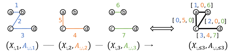
Figure 1: Equivalent snapshotted (left) and aggregated (right) form examples of a 3-time temporal graph without node attributes. Aggregated form collects all edges appeared at least once in snapshotted form, and concatentate corresponding edge attributes into sequences as aggregated edge attributes. If an edge attribute is missing in the concatenation, it will be padded by null attribute 0.

We denote the space of all temporal graphs satisfying either definitions as $\mathbb{T}_{|\mathcal{V}|,T,p}:=\mathbb{R}^{|\mathcal{V}|\times T\times p}\times\mathbb{R}^{|\mathcal{V}|\times|\mathcal{V}|\times T\times p}$.

Next, we will introduce two atomic representations used in both time-and-graph and time-then-graph: GNNs and Recurrent Neural Networks (RNNs).

Our GNN representations follow the Message Passing Neural Network (Gilmer et al., 2017) schema on arbitrary static graph $(\bm{\mathsf{X}},\bm{\mathsf{A}})\in\mathbb{G}_{|\mathcal{V}|,p}$. Formally, the $l$-th layer of a GNN is defined as:

$$\bm{\mathsf{M}}_{i}^{(l)} =\sum\limits_{j\in\mathcal{N}(i)}\text{MSG}^{(l)}\big{(}\bm{\mathsf{Z}}_{i}^{(l-1)},\bm{\mathsf{Z}}_{j}^{(l-1)},\bm{\mathsf{A}}_{i,j}\big{)},$$ (1)

$$\bm{\mathsf{Z}}_{i}^{(l)} =\text{UPDATE}^{(l)}\big{(}\bm{\mathsf{Z}}_{i}^{(l-1)},\bm{\mathsf{M}}_{i}^{(l)}\big{)},$$

where $\bm{\mathsf{Z}}_{i}^{(l)}$ represents the embedding of arbitrary node $i\in\mathcal{V}$ obtained at layer $l$ and $\mathcal{N}(i)$ defines the neighbor set of $i$. We also initialize the corner case $\bm{\mathsf{Z}}_{i}^{(0)}=\bm{\mathsf{X}}_{i}$. $\text{MSG}^{(l)}$ and $\text{UPDATE}^{(l)}$ are arbitrary learnable functions, e.g., Multi-Layer Perceptions (MLPs). For the ease of notation, we denote a stack of $L$ GNN layers by

$$\bm{\mathsf{Z}}^{(L)}=\text{GNN}^{L}(\bm{\mathsf{X}},\bm{\mathsf{A}}),$$ (2)

where all the variables are as in Equation 1. This definition covers widespread GNNs such as GCN (Kipf & Welling, 2016), GAT (Veličković et al., 2018), and GIN (Xu et al., 2018).

Besides GNN as graph representations, sequence representations are also essential in time-and-graph and time-then-graph. In this work we will generally refer to all sequence representation methods as Recurrent Neural Network (RNN) schema which covers widespread methods, e.g., GRU (Cho et al., 2014; Chung et al., 2014) or LSTM (Hochreiter & Schmidhuber, 1997). Strictly speaking, RNN recursively embeds the current and past observations for arbitrary sequence $\bm{\mathsf{S}}\in\mathbb{R}^{T\times p}$ where $p\geq 1$ defines dimension of elements, and is formally defined as:

$$\bm{\mathsf{H}}_{t}=\text{Cell}\big{(}\bm{\mathsf{S}}_{t},\bm{\mathsf{H}}_{t-1}\big{)},$$ (3)

where $\bm{\mathsf{H}}_{t}$ represents the embedding of sub-sequence $\bm{\mathsf{S}}_{1:t}$ for $1\leq t\leq T$. We initialize the corner case $\bm{\mathsf{H}}_{0}=0$. Cell is arbitrary learnable function, e.g., GRU cell. For the ease of notation, we denote RNN on the full sequence as:

$$\bm{\mathsf{H}}_{T}=\text{RNN}(\bm{\mathsf{S}}).$$ (4)

We also consider transformer and other self-attention mechanism methods (Vaswani et al., 2017; Bahdanau et al., 2014), where we define $\bm{\mathsf{H}}_{T}$ as obtained by a set representation instead.

Finally, we will define time-and-graph and time-then-graph methods based on aforementioned input domain and atomic representation concepts.

Time-and-graph. Time-and-graph is the most common representation adopted in the literature. The most widely used time-and-graph representations (e.g., Li et al. (2019); Chen et al. (2018); Seo et al. (2018)) will embed snapshotted temporal graph $\big{[}\big{(}\bm{\mathsf{X}}_{:,t},\bm{\mathsf{A}}_{:,:,t}\big{)}\big{]}_{t=1}^{T}$. First, 1-WL GNNs are independently applied to each snapshot $\big{(}\bm{\mathsf{X}}_{:,t},\bm{\mathsf{A}}_{:,:,t}\big{)}$. Then, the outputs of these GNNs are concatentated and embedded into sequence representations, giving the final representation of all nodes for the temporal graph. Time-and-graph is formally abstracted as:

$$\bm{\mathsf{H}}_{i,t}=\text{Cell}\bigg{(} \Big{[}\text{GNN}_{\text{in}}^{L}\big{(}\bm{\mathsf{X}}_{:,t},\bm{\mathsf{A}}_{:,:,t}\big{)}\Big{]}_{i},$$ (5)

$$\Big{[}\text{GNN}_{\text{rc}}^{L}\big{(}\bm{\mathsf{H}}_{:,t-1},\bm{\mathsf{A}}_{:,:,t}\big{)}\Big{]}_{i}\bigg{)},$$

where $\bm{\mathsf{H}}_{i,t}$ is time-and-graph representation of temporal node $i\in\mathcal{V}$ at time $1\leq t\leq T$. We initialize the corner case $\bm{\mathsf{H}}_{i,0}=0$ for any node $i$. $\text{GNN}_{\text{in}}^{L}$ encodes each snapshot inputs, $\text{GNN}_{\text{rc}}^{L}$ encodes represetations from historical snapshots, and Cell is a RNN cell embedding evolutions of those GNN representations. For an arbitrary temporal graph, the outputs at the last step $\bm{\mathsf{H}}_{i,T}$ is regarded as the final temporal graph representation of node $i\in\mathcal{V}$.

There are several well-known temporal graph works, e.g., Manessi et al. (2020); Sankar et al. (2020); Seo et al. (2018), that fall into a strict subset of defined time-and-graph methods where $\text{GNN}_{\text{rc}}^{L}$ directly outputs its node input $\bm{\mathsf{H}}_{:,t-1}$. We specially call this subset graph-then-time, and it is defined as:

$$\bm{\mathsf{H}}_{i,t}=\text{Cell}\bigg{(}\Big{[}\text{GNN}_{\text{in}}^{L}\big{(}\bm{\mathsf{X}}_{:,t},\bm{\mathsf{A}}_{:,:,t}\big{)}\Big{]}_{i},\bm{\mathsf{H}}_{i,t-1}\bigg{)}$$ (6)

Time-then-graph. This work proposes the time-then-graph framework, which is a more powerful representation than time-and-graph for temporal graphs using 1-WL GNNs. Instead of applying GNNs over each snapshot, we represent the evolution of node attributes using a sequence model. We also perform another sequence representation for the temporal edge attribute evolution. These new node and edge representations become node and edge attributes in a new (static) graph, which is then encoded by a GNN. Thus, our representation architecture will embed aggregated temporal graph $\big{(}\bm{\mathsf{X}}_{:,\leq T},\bm{\mathsf{A}}_{:,:,\leq T}\big{)}$, and it is formally defined as:

$$\bm{\mathsf{H}}^{\text{node}}_{i} =\text{RNN}^{\text{node}}\big{(}\bm{\mathsf{X}}_{i,\leq T}\big{)},\quad\forall i\in\mathcal{V},$$ (7)

$$\bm{\mathsf{H}}^{\text{edge}}_{i,j} =\text{RNN}^{\text{edge}}\big{(}\bm{\mathsf{A}}_{i,j,\leq T}\big{)},\quad\forall(i,j)\in\mathcal{E},$$

$$\bm{\mathsf{Z}} =\text{GNN}^{L}\big{(}\bm{\mathsf{H}}^{\text{node}},\bm{\mathsf{H}}^{\text{edge}}\big{)}.$$

where $\bm{\mathsf{H}}^{\text{node}}$ and $\bm{\mathsf{H}}^{\text{edge}}$ are the representations of node and edge evolutions, $\mathcal{E}$ is the set of all possible edges in aggregated form and $\bm{\mathsf{Z}}$ is final temporal graph representation of all nodes.

State-of-the-art temporal graph representations TGAT and TGN can be treated as special cases of time-then-graph, where $\text{RNN}^{\text{node}}$ and $\text{RNN}^{\text{edge}}$ only takes observable nodes and edges as inputs (subsets of $\bm{\mathsf{X}}_{:,\leq T}$ and $\bm{\mathsf{A}}_{:,:,\leq T}$ with only non-null attributes).

When contrast against time-and-graph, our proposed time-then-graph framework provides following advantages:

1. Time-then-graph with 1-WL GNNs is more expressive than time-and-graph with 1-WL GNNs. Time-then-graph can distinguish different temporal graphs which will always be the same on time-and-graph representation space with 1-WL GNNs. Besides, we show that for any time-and-graph representation, there will be an equivalent counterpart in time-then-graph representation. The expressivity advantage of distinguishing more temporal graphs is empirically beneficial to real-world applications utilizing these representations. We will introduce more details about expressvity in next section.

2. Time-then-graph can be more computationally efficient in practice. GNNs often operate on sparse temporal graphs, and could benefit a lot from parallel computation. In time-and-graph framework, there is a bottleneck that $\text{GNN}^{L}_{\text{rc}}$ must wait for $\bm{\mathsf{H}}_{:,t-1}$ until all previous snapshots are processed. Thus, time-and-graph must process snapshots one-by-one, which does not fully utilize parallelization. In contrast, there is not such bottleneck in time-then-graph, both RNNs and GNNs can compute many of the embeddings in parallel during their time and graph phase, respectively. We empirically show that our time-then-graph methods train faster than all baselines in real-world tasks when the number of temporal edges is not large.

3 Expressivity of Equivariant Temporal Graph Representations

In this section, we will discuss more details about the expressivity advantage of time-then-graph over time-and-graph. First, however, we will clarify the concept of expressivity.

In the following analysis, we will treat the representation of an arbitrary domain $\mathcal{U}$ as a function $f:\mathcal{U}\rightarrow\mathbb{R}^{d}$ which embeds any element from $\mathcal{U}$ into a low-dimensional vector on $\mathbb{R}^{d}$, where $d\geq 1$ is the representation space dimensionality. For example, a specific GNN architecture defines a family of representations $\mathcal{F}$ for domain $\mathcal{U}=\mathbb{G}_{|\mathcal{V}|,p}$, and a specific function $f\in\mathcal{F}$ defines a specific set of parameters for such GNN architecture. Similarly, TGNNs defines a family of representations $\mathcal{F}^{\prime}$ representations for domain $\mathcal{U}=\mathbb{T}_{|\mathcal{V}|,T,p}$.

In static and temporal graph expressvity studies (Xu et al., 2018; Maron et al., 2019b; Morris et al., 2019; Murphy et al., 2019; Azizian & Lelarge, 2020; Kileel et al., 2019; Kapoor et al., 2020), the expressivity of a representation $f$ for an arbitrary domain $\mathcal{U}$ is represented by the cardinality of distinguishable inputs on its representation space. To help understand this concept, we describe identifiable set, which is then used to define the expressivity of representations on arbitrary domain.

Definition 3.1 (Identifiable Set).

The identifiable set $\mathcal{I}(f,\mathcal{U})$ of a representation $f$ with domain $\mathcal{U}$ is a set s.t.:

1. It is a subset of $\mathcal{U}$ that is $\mathcal{I}(f,\mathcal{U})\subseteq\mathcal{U}$;

2. None of its elements have the same representations, that is $\forall\bm{u}_{1}\neq\bm{u}_{2}\in\mathcal{I}(f,\mathcal{U}),f\big{(}\bm{u}_{1}\big{)}\neq f\big{(}\bm{u}_{2}\big{)}$;

3. It contains all unique representations over domain $\mathcal{U}$, that is, $\forall\bm{u}_{1}\in\mathcal{U}\backslash\mathcal{I}(f,\mathcal{U}),\exists\bm{u}_{2}\in\mathcal{I}(f,\mathcal{U}),f\big{(}\bm{u}_{1}\big{)}=f\big{(}\bm{u}_{2}\big{)}$.

In other words, $\mathcal{I}(f,\mathcal{U})$ is the maximal subset of $\mathcal{U}$ that $f$ can differentiate any pair of elements in that domain. We may have multiple identifiable sets satisfying Definition 3.1 for the same representation $f$ with domain $\mathcal{U}$. We find that for any pair of such identifiable sets, there are always bijection between them. Thus, all satisfying identifiable sets are equivalent in the sense of cardinality on representation space, thus we can use an arbitrary identifiable set for later expressivity analysis. We provide a proof of the bijection in Section A.1.

Node isomorphism. When studying the second condition of Definition 3.1 in graph domains, where $\bm{u}_{1},\bm{u}_{2}$ are two graphs, we define equality $\bm{u}_{1}=\bm{u}_{2}$ as having graphs $\bm{u}_{1}$ and $\bm{u}_{2}$ being isomorphic. We say two temporal graphs are isomorphic if their aggregation forms (Definition 2.3) are isomorphic.

We now define the expressivity of representations on an arbitrary domain $\mathcal{U}$ based on identifiable set. Since we eventually want to compare the expressivity between time-and-graph and time-then-graph which are two families of representations, we formally quantify the expressivity comparison between two arbitrary representation familes on the same domain.

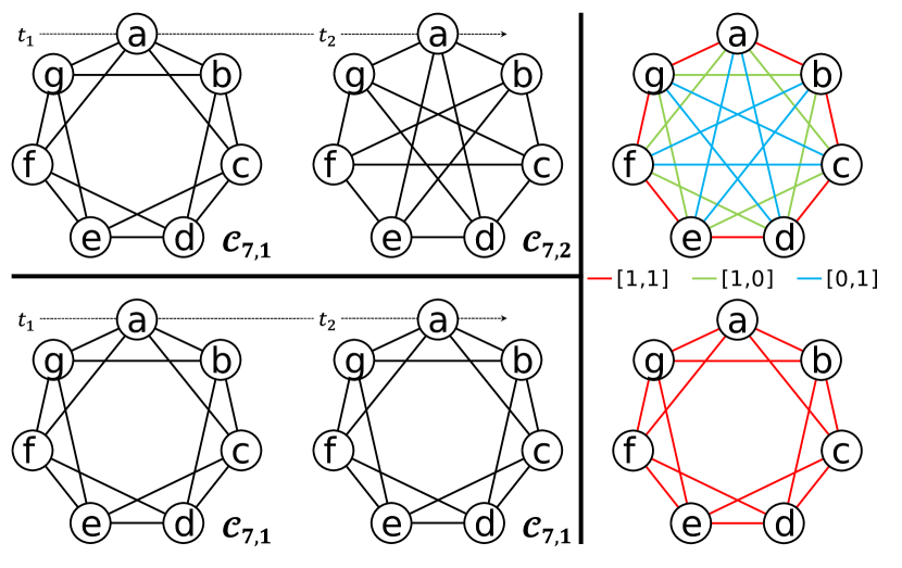
Figure 2: A synthetic task where only time-then-graph is expressive enough with 1-WL GNNs. The top and bottom 2-time temporal graphs on the left side has snapshots of different structure at time $t_{2}$ (denote by $\mathcal{C}_{7,2}$ and $\mathcal{C}_{7,1}$). The two aggregated temporal graphs on the right side are corresponding aggregation of two snapshotted forms, where edge attributes are sequences of non-existing (0) and existing (1) over time, denoted by different colors. The task is to distinguish structure difference between top and bottom temporal graphs. Time-and-graph using 1-WL GNNs will fail since GNN always output the same node representation for both snapshot $\mathcal{C}_{7,2}$ and $\mathcal{C}_{7,1}$ (see (Murphy et al., 2019)). On the other hand, time-then-graph works since the aggregated forms already show different aggregated topologies that any 1-WL GNN can easily distinguish.

Definition 3.2 (Quantifying Levels of Expressivity).

Consider two representation families $\mathcal{F}_{1}$ and $\mathcal{F}_{2}$ of domain $\mathcal{U}$. We say $\mathcal{F}_{1}$ is more or as equally expressive as $\mathcal{F}_{2}$, if and only if $\exists f_{1}\in\mathcal{F}_{1}$, $\forall f_{2}\in\mathcal{F}_{2},\big{|}\mathcal{I}\big{(}f_{2},\mathcal{U}\big{)}\big{|}\leq\big{|}\mathcal{I}\big{(}f_{1},\mathcal{U}\big{)}\big{|}$. We denote this by $\mathcal{F}_{2}\preceq_{\mathcal{U}}\mathcal{F}_{1}$.
It is strictly more expressive, $\mathcal{F}_{2}\precneqq_{\mathcal{U}}\mathcal{F}_{1}$, if and only if $\exists f_{1}\in\mathcal{F}_{1}$, $\forall f_{2}\in\mathcal{F}_{2},\big{|}\mathcal{I}\big{(}f_{2},\mathcal{U}\big{)}\big{|}<\big{|}\mathcal{I}\big{(}f_{1},\mathcal{U}\big{)}\big{|}$.
If two representation families satisfies both $\mathcal{F}_{2}\preceq_{\mathcal{U}}\mathcal{F}_{1}$ and $\mathcal{F}_{1}\preceq_{\mathcal{U}}\mathcal{F}_{2}$, we say that they are equally expressive, $\mathcal{F}_{2}\stackrel{{\scriptstyle e}}{{=}}_{\mathcal{U}}\mathcal{F}_{1}$.

Definition 3.3 (Most Expressive).

A representation family $\mathcal{F}^{+}$ for $\mathcal{U}$ is the most expressive representation family if and only if $\forall\bm{u}_{1},\bm{u}_{2}\in\mathcal{U}$, $\exists f^{+}\in\mathcal{F}^{+}$, $f^{+}\big{(}\bm{u}_{1}\big{)}=f^{+}\big{(}\bm{u}_{2}\big{)}\Longleftrightarrow\bm{u}_{1}=\bm{u}_{2}$. We call such $f^{+}$ as the most expressive representation function.

Generally speaking, more expressive representation family means that the architecture $\mathcal{F}$ is being able to better distinguish distinct elements in domain $\mathcal{U}$, and most expressive representation family means being able to distinguish all distinct elements in domain $\mathcal{U}$.

Lemma 3.4 (Expressivity & Representations).

For two representation families $\mathcal{F}_{1}$ and $\mathcal{F}_{2}$ of domain $\mathcal{U}$, if for any function of $\mathcal{F}_{2}$, there is an equivalent function on $\mathcal{U}$ in $\mathcal{F}_{1}$, then $\mathcal{F}_{2}\preceq_{\mathcal{U}}\mathcal{F}_{1}$, that is,

$$\forall f_{2}\in\mathcal{F}_{2},\exists f_{1}\in\mathcal{F}_{1},\text{ s.t. }\forall\bm{u}\in\mathcal{U},f_{1}(\bm{u})=f_{2}(\bm{u})$$

$$\Longrightarrow\mathcal{F}_{2}\preceq_{\mathcal{U}}\mathcal{F}_{1}.$$

Lemma 3.4 is straightforward: If $\mathcal{F}_{1}$ can simulate any representation function in $\mathcal{F}_{2}$ on domain $\mathcal{U}$, then it distinguish at least the same elements. It also reveals a more direct way to compare expressivity between representation families than cardinality, and we will adopt this in the expressivity comparison between time-and-graph and time-then-graph.

Now that we have formally defined the concept of expressivity, and can analyze the expressivity of time-and-graph and time-then-graph frameworks. To start, we need to understand the expressivity of their components, GNNs and RNNs, which has already been sufficiently explored in the literature. Thus, we can directly take expressivity conclusions from existing works:

1. Common message passing GNNs including GCN (Kipf & Welling, 2016), GAT (Veličković et al., 2018), and GIN (Xu et al., 2018) are the same expressive as 1-Weisfeiler-Lehman (1-WL) test (Leman & Weisfeiler, 1968; Douglas, 2011; Xu et al., 2018; Morris et al., 2019), which are NOT the most expressive graph representation.

2. There are more expressive GNNs than 1-WL GNNs, e.g., k-WL GNNs (Morris et al., 2019). The most expressive GNNs, denoting as GNN⁺, also exist (Maron et al., 2019b; Murphy et al., 2019). However, all of them are not as efficient as 1-WL, thus is not widely used.

3. RNNs can be most expressive sequence representations (Siegelmann & Sontag, 1995; Yun et al., 2020). GRU (Chung et al., 2014), LSTM (Hochreiter & Schmidhuber, 1997) and transformer (Vaswani et al., 2017) architectures are most expressive RNNs in this paper.

To differentiate temporal graph representations using GNNs of different expressivities, we replace the graph by exact type of GNNs, e.g., time-then-graph with 1-WL GNNs is denoted as time-then-1WLGNN. We derive the expressivity of temporal graphs based on aforementioned conclusions.

Theorem 3.5.

[Temporal 1-WL Expressivity] Time-then-graph is strictly more expressive than time-and-graph representation family on $\mathbb{T}_{|\mathcal{V}|,T,p}$ when the graph representation is a 1-WL GNN:

$$\text{{\em 1WLGNN-then-time}}\precneqq_{\mathbb{T}_{|\mathcal{V}|,T,p}}\text{{\em time-and-1WLGNN}}$$

$$\precneqq_{\mathbb{T}_{|\mathcal{V}|,T,p}}\text{{\em time-then-1WLGNN}}.$$

In Section A.2, we prove this by showing that we can always construct a time-then-graph representation that outputs the same embeddings as an arbitrary time-and-graph representation. Thus, by Lemma 3.4, time-then-graph is as expressive as time-and-graph. We also provide a task in Figure 2 where any time-and-graph representation will fail while a time-then-graph would work, which then, added to the previous result, proves that time-then-graph is strictly more expressive than time-and-graph.

Theorem 3.6.

[Temporal GNN Expressivity] Using more expressive GNNs, e.g., kWL GNNs, will improve the expressivity of time-then-graph, and if a most expressive GNN⁺ is used, time-then-graph and time-and-graph representation families will both be most expressive:

$$\text{{\em time-then-1WLGNN}}\precneqq_{\mathbb{T}_{|\mathcal{V}|,T,p}}\text{{\em time-then-$k$WLGNN}}$$

$$\precneqq_{\mathbb{T}_{|\mathcal{V}|,T,p}}\text{{\em time-then-GNN${}^{+}$}}\stackrel{{\scriptstyle e}}{{=}}_{\mathbb{T}_{|\mathcal{V}|,T,p}}\text{{\em time-and-GNN${}^{+}$}}.$$

A proof of this is also provided in Section A.3.

Theorems 3.5 and 3.6 show that time-then-graph is more expressive than time-and-graph as long as we must use 1-WL GNNs, but they are indeed equivalent when most expressive GNNs are available.

4 Related Work

Time-and-graph. GCRN-M2 (Seo et al., 2018) is the first work, as far as we know, to adopt Equation 5 combining SpectralGCN (Defferrard et al., 2016) and LSTM. DCRNN (Li et al., 2018) is a time-and-graph application in traffic forecasting utilizing SpectralGCN and GRU. LRGCN (Li et al., 2019) is another similar work but has further processing on node representations. GGNN (Li et al., 2016) is a time-and-graph application where node attributes do not change, thus it removes $\text{GNN}_{\text{in}}$ that most time-and-graph methods have.

Graph-then-time. The framework defined by Equation 6 is the most popular among both traditional and state-of-the-art works for its simplicity and efficiency. Seo et al. (2018) proposes GCRN-M1 in the same paper of GCRN-M2 but GCRN-M1 uses a graph-then-time framework. Manessi et al. (2020) also proposes something similar, WD-GCN, which combines GCN and LSTM through a graph-then-time framework. Another state-of-the-art work, DySAT (Sankar et al., 2020), exploits self-attention mechanism of GAT (Veličković et al., 2018) and a transformer (Vaswani et al., 2017) via graph and sequence components. Of special interest is EvolveGCN (Pareja et al., 2020), which learns the temporal dynamics through the GCN parameters rather than node representations. In EvolveGCN, GCN parameters are passed as recurrent states instead of historical embeddings. DynGEM (Goyal et al., 2018) is similar to EvolveGCN, but it directly inherits parameters from previous step instead of an RNN to model parameter evolution.

Time-then-graph. To the best of our knowledge, the first time-then-graph work is Rahman et al. (2018), which only uses non-parametric graph and sequence components. Two other works, TGAT (da Xu et al., 2020) and TGN (Rossi et al., 2020), are existing state-of-the-art time-then-graph works. Instead of accumulating even non-existing edge attributes, they simply collect all observed edges in past snapshots, and extract static graph representations from a heterogeneous graph constructed through those edges. THINE (Huang et al., 2021) and CAW (Wang et al., 2021) are works close to TGAT but use random walks for label propagation instead of GNNs. Makarov et al. (2021) uses the same procedure as CAW but applied to TGN. Our time-then-graph method differ from the above methods, since we distill the time-then-graph framework into its basic components: A powerful temporal representation (e.g., a GRU) and a good 1-WL GNN graph representation.

Table 1: Statistics of datasets. We collect and denote the number of samples (temporal graphs) as $N$, number of nodes as $|\mathcal{V}|$, minimum and maximum number of edges for all snapshots as $\min_{t}\big{|}\mathcal{E}_{t}\big{|}$ and $\max_{t}\big{|}\mathcal{E}_{t}\big{|}$, number of snapshots per sample (temporal graph) as $T$, node and edge attribute dimensionality as $\big{|}p_{\bm{\mathsf{X}}}\big{|},\big{|}p_{\bm{\mathsf{A}}}\big{|}$, learning target dimensionality as $|\mathbf{y}|$ and number of graphs per minibatch as $B$.

Dataset	$N$	$|\mathcal{V}|$	$\min_{t}\big{|}\mathcal{E}_{t}\big{|}$	$\max_{t}\big{|}\mathcal{E}_{t}\big{|}$	$T$	$\big{|}p_{\bm{\mathsf{X}}}\big{|}$	$\big{|}p_{\bm{\mathsf{A}}}\big{|}$	$|\mathbf{y}|$	$B$
DynCSL	200	19	76	76	8	0	0	1	1
Brain10	1	5000	154094	167944	12	20	0	1	1
PeMS04	16980	307	680	680	12	5	1	3	256
PeMS08	17844	170	548	548	12	5	1	3	256
Spain-COVID	443	52	7030	7030	7	1	2	1	64
English-COVID	54	129	836	2158	7	1	1	1	4

Permutation-sensitive TGNNs. There are several temporal graph works that consider permutation-sensitive (non-equivariant) graph representations. DynAERNN (Goyal et al., 2020) uses adjacency vector of each node as augmented node feature; AdaNN-D (Xu et al., 2019) uses the random walk vector based on adjacency matrix as augmented node feature; E-LSTM-D (Chen et al., 2019a) uses flattened adjacency matrix as augmented input of LSTM; and GC-LSTM (Chen et al., 2018) directly uses adjacency matrix as augmented input of LSTM. All aforementioned works share the same challenge: If we permute node indices, resulting in a different adjacency matrix of an isomorphic graph, their final node representation changes. This is a property we want to avoid in node and graph tasks (classification and regression).

Extension of Temporal Graph Representations. Recent works also merge existing TGNNs with new representation tuning techniques. Hajiramezanali et al. (2019) incorporates variable autoencoder into time-and-graph. Lei et al. (2019); Xiong et al. (2019) incorporates time-and-graph under an adversarial learning framework. Similarly, HTGN (Yang et al., 2021) is a graph-then-time representation in hyperbolic space. Although these variants provide new applications for temporal graph representations, they do not improve the expressivity of the time-and-graph framework.

Table 2: Performance on temporal graph and node classification tasks. Performance is evaluated by ROCAUC score where higher value means better performance. Best mean performance is both bolded and underlined, and the second best one is only bolded. Our proposed GCN-GRU is the only one works on DynCSL dataset, and is placed at the top with another time-then-graph model, TGN, on Brain10 dataset.

Representation	Model	DynCSL	Brain-10
graph-then-time	EvolveGCN-O	$0.50{\scriptstyle\pm 0.00}$	$0.58{\scriptstyle\pm 0.10}$
	EvolveGCN-H	$0.50{\scriptstyle\pm 0.00}$	$0.60{\scriptstyle\pm 0.11}$
	GCN-GRU	$0.50{\scriptstyle\pm 0.00}$	$0.87{\scriptstyle\pm 0.07}$
	DySAT	$0.50{\scriptstyle\pm 0.00}$	$0.77{\scriptstyle\pm 0.07}$
time-and-graph	GCRN-M2	$0.52{\scriptstyle\pm 0.04}$	$0.77{\scriptstyle\pm 0.04}$
	DCRNN	$0.51{\scriptstyle\pm 0.03}$	$0.84{\scriptstyle\pm 0.02}$
time-then-graph	TGAT	$0.48{\scriptstyle\pm 0.03}$	$0.80{\scriptstyle\pm 0.03}$
	TGN	$0.51{\scriptstyle\pm 0.04}$	$\mathbf{0.91{\scriptstyle\pm 0.03}}$
	GRU-GCN	$\mathbf{1.00{\scriptstyle\pm 0.00}}$	$\mathbf{0.91{\scriptstyle\pm 0.03}}$

Table 3: Performance on temporal node regression tasks. Performance is evaluated by MAPE (%) where lower value means better performance (see Equation 18 in Section B.3). Best mean performance is both bolded and underlined, and the second best one is only bolded. Our proposal GCN-GRU is always the best one on all inductive learnings. On transductive tasks, our proposal is the best on PeMS08 and England-COVID datasets, and is the second best on PeMS04 and Spain-COVID datasets. Time-then-graph representations can always provide the best performance with only one exception for transductive learning on PeMS04 where it is only the second best.

Representation	Model	PeMS04		PeMS08		Spain-COVID		England-COVID
		Transductive	Inductive	Transductive	Inductive	Transductive	Inductive	Transductive	Inductive
graph-then-time	EvolveGCN-O	$3.20{\scriptstyle\pm 0.25}$%	$2.61{\scriptstyle\pm 0.42}$%	$2.65{\scriptstyle\pm 0.12}$%	$2.40{\scriptstyle\pm 0.27}$%	$2.64{\scriptstyle\pm 0.12}$%	$2.02{\scriptstyle\pm 0.11}$%	$4.07{\scriptstyle\pm 0.73}$%	$3.88{\scriptstyle\pm 0.47}$%
	EvolveGCN-H	$3.34{\scriptstyle\pm 0.14}$%	$2.84{\scriptstyle\pm 0.31}$%	$2.81{\scriptstyle\pm 0.28}$%	$2.81{\scriptstyle\pm 0.23}$%	$2.62{\scriptstyle\pm 0.33}$%	$2.09{\scriptstyle\pm 0.30}$%	$4.14{\scriptstyle\pm 1.14}$%	$3.50{\scriptstyle\pm 0.42}$%
	GCN-GRU	$\mathbf{1.60{\scriptstyle\pm 0.14}}$%	$1.28{\scriptstyle\pm 0.04}$%	$1.40{\scriptstyle\pm 0.26}$%	$1.07{\scriptstyle\pm 0.03}$%	$2.39{\scriptstyle\pm 0.06}$%	$1.22{\scriptstyle\pm 0.66}$%	$\mathbf{3.56{\scriptstyle\pm 0.26}}$%	$\mathbf{2.97{\scriptstyle\pm 0.34}}$%
	DySAT	$1.86{\scriptstyle\pm 0.08}$%	$1.58{\scriptstyle\pm 0.08}$%	$1.49{\scriptstyle\pm 0.08}$%	$1.34{\scriptstyle\pm 0.03}$%	$2.15{\scriptstyle\pm 0.18}$%	$\mathbf{0.89{\scriptstyle\pm 0.44}}$%	$3.67{\scriptstyle\pm 0.15}$%	$3.32{\scriptstyle\pm 0.76}$%
time-and-graph	GCRN-M2	$1.70{\scriptstyle\pm 0.20}$%	$1.20{\scriptstyle\pm 0.06}$%	$\mathbf{1.30{\scriptstyle\pm 0.17}}$%	$1.00{\scriptstyle\pm 0.10}$%	$1.94{\scriptstyle\pm 0.54}$%	$1.54{\scriptstyle\pm 0.50}$%	$3.85{\scriptstyle\pm 0.39}$%	$3.37{\scriptstyle\pm 0.27}$%
	DCRNN	$1.67{\scriptstyle\pm 0.19}$%	$1.27{\scriptstyle\pm 0.06}$%	$1.32{\scriptstyle\pm 0.19}$%	$1.07{\scriptstyle\pm 0.03}$%	$2.12{\scriptstyle\pm 0.33}$%	$0.90{\scriptstyle\pm 0.21}$%	$3.58{\scriptstyle\pm 0.53}$%	$3.09{\scriptstyle\pm 0.24}$%
time-then-graph	TGAT	$3.11{\scriptstyle\pm 0.50}$%	$2.25{\scriptstyle\pm 0.27}$%	$2.66{\scriptstyle\pm 0.27}$%	$2.34{\scriptstyle\pm 0.19}$%	$2.46{\scriptstyle\pm 0.04}$%	$1.81{\scriptstyle\pm 0.14}$%	$5.44{\scriptstyle\pm 0.46}$%	$5.13{\scriptstyle\pm 0.26}$%
	TGN	$1.79{\scriptstyle\pm 0.21}$%	$\mathbf{1.19{\scriptstyle\pm 0.07}}$%	$1.49{\scriptstyle\pm 0.26}$%	$\mathbf{0.99{\scriptstyle\pm 0.06}}$%	$\mathbf{1.62{\scriptstyle\pm 0.33}}$%	$1.25{\scriptstyle\pm 0.48}$%	$4.15{\scriptstyle\pm 0.81}$%	$3.17{\scriptstyle\pm 0.23}$%
	GRU-GCN	$\mathbf{1.61{\scriptstyle\pm 0.35}}$%	$\mathbf{1.13{\scriptstyle\pm 0.05}}$%	$\mathbf{1.27{\scriptstyle\pm 0.21}}$%	$\mathbf{0.89{\scriptstyle\pm 0.07}}$%	$\mathbf{1.66{\scriptstyle\pm 0.63}}$%	$\mathbf{0.65{\scriptstyle\pm 0.16}}$%	$\mathbf{3.41{\scriptstyle\pm 0.28}}$%	$\mathbf{2.87{\scriptstyle\pm 0.19}}$%

5 Experiments

In this section, we evaluate a simple architecture based on our time-then-graph framework on one synthetic dataset and five different real-world datasets. We also evaluate eight state-of-the-art temporal graph representation baselines on the same tasks. Each experiment is repeated ten times with different random initialization. Please refer to the Appendix B for a detailed description of experiment setup, and to our code for hyperparameter configurations .

Learning tasks. In this work, all the learning tasks will use equivariant temporal graph representations as described in Section 3. It is known that equivariant graph representations are generally not sufficiently expressive for prediction tasks beyond node and graph (structure) predictions, especially for edge-level tasks such as link prediction (Srinivasan & Ribeiro, 2020; You et al., 2019) and shortest path estimation (Dehmamy et al., 2019; Loukas, 2020; Tang et al., 2020). Indeed, equivariant temporal graph representations inherit the same expressivity insufficiency, thus are also improper for edge-level tasks. A formal explanation of this limitation is provided in Section A.5. Thus, to deliver theoretically sound experiments, we only consider temporal graph classification, node classification and node regression as learning tasks in our experiments.

DynCSL. DynCSL is a synthetic temporal graph classification task. Each sample is constructed by a sequence of 8 graph snapshots. Each snapshot is randomly drawed from $\big{\{}\mathcal{C}_{19,2},\cdots,\mathcal{C}_{19,6}\big{\}}$. Here, $\mathcal{C}_{|\mathcal{V}|,s}$ means a Circular Skip Link (CSL) (Murphy et al., 2019) graph with $|\mathcal{V}|$ nodes and skip length $s$. A CSL sequence example is introduced Figure 2. The goal is to predict the number of unique non-isomorphic CSLs in the constructed temporal graph, e.g., the top temporal graph in Figure 2 has prediction “2”, while the bottom one has prediction “1”. DynCSL is a temporal extension of the CSL task. CSL is widely used as a first-test of the expressiveness of static GNNs (Bodnar et al., 2021; Chen et al., 2019; Cotta et al., 2021; Dwivedi et al., 2020; Nguyen & Maehara, 2020; Tiezzi et al., 2021; Zhang et al., 2021).

Real-world applications. We also evaluate the performace on several real-word applcations including a brain functionality classification Brain10, two traffic forecasting PeMS04 and PeMS08, and two COVID spreading prediction Spain-COVID and England-COVID.

Generally speaking, our data consists of a set of temporal graphs. These temporal graphs are defined over the same set of nodes. For instance, a temporal graph may represent the evolution of a system in a day, while the different temporal graphs would represent different days. Please refer to Section B.4 for a in-depth description of our datasets, whose general statistics are shown in Table 1.

Our model and baselines. We compare an representation instance of our time-then-graph approach, GRU-GCN, with 5 time-and-graph methods (namely, EvolveGCNs, GCN-GRU, DySAT, GCRN-M2 and DCRNN) and two time-then-graph methods (namely, TGAT and TGN). Our proposal GRU-GCN means using GRUs for both node and edge sequence representations and GCN as graph representation in time-then-graph framework as Equation 7. All baselines have been briefly introduced in Section 4. Please refer to Appendix B for details about architectures of all models.

Table 4: Resource cost of tasks on GPUs. We collect the peak GPU memory and average training time per minibatch from all tasks utilizing GPU resources on a GeForce RTX 2080 Ti. Best training time efficency is both bolded and underlined. Our proposal GCN-GRU are always the most time efficent method for GPUs on all four tasks. Furthermore, it uses the least GPU memory among all state-of-the-art time-then-graph representation methods.

Representation	Model	PeMS04		PeMS08		Spain-COVID		England-COVID
		Peak GPU Memory	Average Training Time per Minibatch	Peak GPU Memory	Average Training Time per Minibatch	Peak GPU Memory	Average Training Time per Minibatch	Peak GPU Memory	Average Training Time per Minibatch
graph-then-time	EvolveGCN-O	86 MB	19ms	55 MB	17 ms	221 MB	14 ms	3MB	9 ms
	EvolveGCN-H	205 MB	40 ms	130 MB	31 ms	512 MB	21 ms	4 MB	15 ms
	GCN-GRU	1089 MB	17 ms	602 MB	15 ms	140 MB	12 ms	6 MB	8 ms
	DySAT	1911 MB	26 ms	1060 MB	24 ms	137 MB	18 ms	7 MB	14 ms
time-and-graph	GCRN-M2	3099 MB	195 ms	1871 MB	159 ms	5423 MB	124 ms	22 MB	84 ms
	DCRNN	1730 MB	83 ms	1024 MB	65 ms	2460 MB	50 ms	13 MB	34 ms
time-then-graph	TGAT	7945 MB	101 ms	5680 MB	72 ms	7300 MB	94 ms	96 MB	21 ms
	TGN	3963 MB	25 ms	2908 MB	19 ms	5205 MB	29 ms	73 MB	16 ms
	GRU-GCN	859 MB	7 ms	574 MB	5 ms	1538 MB	10 ms	52 MB	3 ms

5.1 Performance on tasks that mostly depend on the evolving topology

First, we analyze the performance of our model against other baselines on DynCSL and Brain10 datasets whose prediction are highly dependent to temporal topologies in Table 2. DynCSL is an extension of the task in the proof of Theorem 3.5 where our method is strictly more expressive than time-and-graph on classifying temporal topologies. For Brain10, the functionality of brain voxel is mostly determined by its activations with other voxels which are mostly covered in its temporal topologies, thus we also expect our proposal to perform better than time-and-graph baselines on it.

Indeed, our GRU-GCN time-then-graph architecture is the only method that works on the DynCSL task, while all the other baselines —including two state-of-the-art time-then-graph methods— give performances no better than random predictions. This observation follows the time-then-graph expressivity advantage introduced in Figure 2. Notably, the result also reflects our proposed GRU-GCN also holds expressivity advantage over the other two time-then-graph methods, TGAT and TGN. This advantage is caused by taking not-existing edge attributes into consideration in our model while TGAT and TGN only collects existing edge attributes. Please refer to Section A.4 for formal explanation of this observation.

Our time-then-graph GRU-GCN is also one of the top methods on Brain10, with TGN as the only competitor of the same performance. These two are both under time-then-graph framework, and gain a clear improvement from time-and-graph baselines. This observation provides a further evidence on expressivity advantage of time-then-graph over time-and-graph. The exception is TGAT, which is not performing ideally in both cases. The reason is that there is no sequence representation used in TGAT which plays a key role in time-then-graph framework, thus TGAT is more like a static GNN baseline but on heterogeneous graph rather than a temporal graph method which limits its power compared to other temporal graph representations.

5.2 Performance on tasks where attribute evolution is more relevant

Table 2 summarizes the result over all remaining real-world datasets. Each dataset is further split into two different tasks: Transductive learning, where two disjoint sets of nodes of a temporal graph are selected for validation and test. At the last snapshot, the attributes of nodes in validation and test data are hidden from us during training. Inductive learning, where in training we have access to full data (all node and edges attributes over all snapshots) for some temporal graphs (training graphs). In test, for a new set of unseen temporal graphs, we are asked to predict all node attributes of the last snapshot given past snapshots.

Table 3 shows that our proposed time-then-graph GRU-GCN is often the best model on all tasks (tansductive and inductive), with only two exceptions: Transductive PeMS04 and Spain-COVID where our proposal is still the second best model and very close to the best performance. This is somewhat expected since the rich variation on real-world node and edge attributes in these datasets can reduce the expressivity advantage of time-then-graph over time-and-graph.

5.3 Empirical computational efficiency

While theoretically we do not expect computational efficiency gains from time-then-graph methods over time-and-graph methods (see Section B.2), in practice we observe reasonable gains in some datasets. In order to study the real-world computational efficiency of our approach on GPUs, we collect the peak GPU memory cost and average training time cost per minibatch for datasets utilizing GPU resources. We do not collect GPU data for Brain10 since its graph is too large to fit in GPU memory for our comparisons.

The runtime data in Table 4 shows that our GRU-GCN proposal is consistently the fastest method in all datasets. Furthermore, it also requires the least amount of memory among all time-then-graph methods. This efficiency advantage is caused by small number of edges for studying datasets, which results in small cost for RNN on edge attributes. However, if the aggregated temporal graph is dense, time-then-graph will no longer be as efficient. We provide more details in Section B.5.

6 Conclusion and Future Work

We proposed time-then-graph, an alternative representation framework for temporal graphs for node and graph classification and regression tasks. While time-and-graph (and its variant graph-then-time) are still the most widely-used frameworks for temporal graphs, we formally prove that our proposed time-then-graph framework is more expressive than time-and-graph if the graph representation uses the ubiquitous 1-WL GNN architecture. Our experiments confirm this expressivity gain, achieving state-of-the-art performance on synthetic and real-world tasks. Overall, time-then-graph provides a new ML tool for temporal graph applications.

Appendix A Proves

A.1 Identifiable Set Equivalence

Lemma A.1 (Identifiable Set Equivalence).

Suppose $\mathcal{I}_{1}(f,\mathcal{U})$ and $\mathcal{I}_{2}(f,\mathcal{U})$ are two identifiable sets of representation function $f$ on domain $\mathcal{U}$, then there exists a bijection between $\mathcal{I}_{1}(f,\mathcal{U})$ and $\mathcal{I}_{2}(f,\mathcal{U})$ based on matching between representations.

Proof.

We show this by contradiction. Assume that there is no such bijection by matching representations between $\mathcal{I}_{1}(f,\mathcal{U})$ and $\mathcal{I}_{2}(f,\mathcal{U})$. Without loss of generality, suppose there is an element $\bm{u}_{1}\in\mathcal{I}_{1}(f,\mathcal{U})$ such that no element from $\mathcal{I}_{2}(f,\mathcal{U})$ can match its representation, in other words, $\exists\bm{u}_{1}\in\mathcal{I}_{1}(f,\mathcal{U}),\forall\bm{u}_{2}\in\mathcal{I}_{2}(f,\mathcal{U}),f\big{(}\bm{u}_{1}\big{)}\neq f\big{(}\bm{u}_{2}\big{)}$. This implies $\bm{u}_{1}\notin\mathcal{I}_{2}(f,\mathcal{U})$, otherwise $\bm{u}_{1}\in\mathcal{I}_{2}(f,\mathcal{U})$ will match with $\bm{u}_{1}\in\mathcal{I}_{1}(f,\mathcal{U})$ on representations. Thus, $\bm{u}_{1}\in\mathcal{U}-\mathcal{I}_{2}(f,\mathcal{U})$. According to Definition 3.1, for $\bm{u}_{1}\in\mathcal{U}-\mathcal{I}_{2}(f,\mathcal{U})$, $\exists\bm{u}^{\prime}_{2}\in\mathcal{I}_{2}(f,\mathcal{U}),f\big{(}\bm{u}_{1}\big{)}=f\big{(}\bm{u}^{\prime}_{2}\big{)}$. This leads to a contradiction since we assume that no elements from $\mathcal{I}_{2}(f,\mathcal{U})$ can match with $\bm{u}_{1}$ on its representation $f\big{(}\bm{u}_{1}\big{)}$, but we find matching $\bm{u}^{\prime}_{2}\in\mathcal{I}_{2}(f,\mathcal{U})$.

So, for any elements in $\mathcal{I}_{1}(f,\mathcal{U})$, there must exists an element in $\mathcal{I}_{2}(f,\mathcal{U})$ matching its representation. And, this mapping is an injection from $\mathcal{I}_{1}(f,\mathcal{U})$ to $\mathcal{I}_{2}(f,\mathcal{U})$ since $\mathcal{I}_{1}(f,\mathcal{U})$ does not contain elements of the same representation based on Definition 3.1. The same applies flipping the roles of $\mathcal{I}_{2}(f,\mathcal{U})$ and $\mathcal{I}_{1}(f,\mathcal{U})$.

Hence, by the Schröder-Bernstein theorem, if there is an injection from $\mathcal{I}_{1}(f,\mathcal{U})$ to $\mathcal{I}_{2}(f,\mathcal{U})$ and an injection from $\mathcal{I}_{2}(f,\mathcal{U})$ to $\mathcal{I}_{1}(f,\mathcal{U})$, then there is a bijection between $\mathcal{I}_{1}(f,\mathcal{U})$ and $\mathcal{I}_{2}(f,\mathcal{U})$.

∎

A.2 Temporal 1-WL Expressivity

See 3.5

Proof.

Roadmap: We first show that we can construct an equivalent time-then-1WLGNN representation for any time-and-1WLGNN representation on arbitrary temporal graph domain $\mathbb{T}_{|\mathcal{V}|,T,p}$. Thus, according to Lemma 3.4, time-then-1WLGNN is at least as expressive as time-and-1WLGNN. Furthermore, we provide an instance where time-and-1WLGNN fails to distinguish two different temporal graphs but time-then-1WLGNN can. This further shows that time-then-1WLGNN is strictly more expressive, in other words,

$$\text{{\em Time-and-1WLGNN}}\precneqq_{\mathbb{T}_{|\mathcal{V}|,T,p}}\text{{\em Time-then-1WLGNN}}.$$

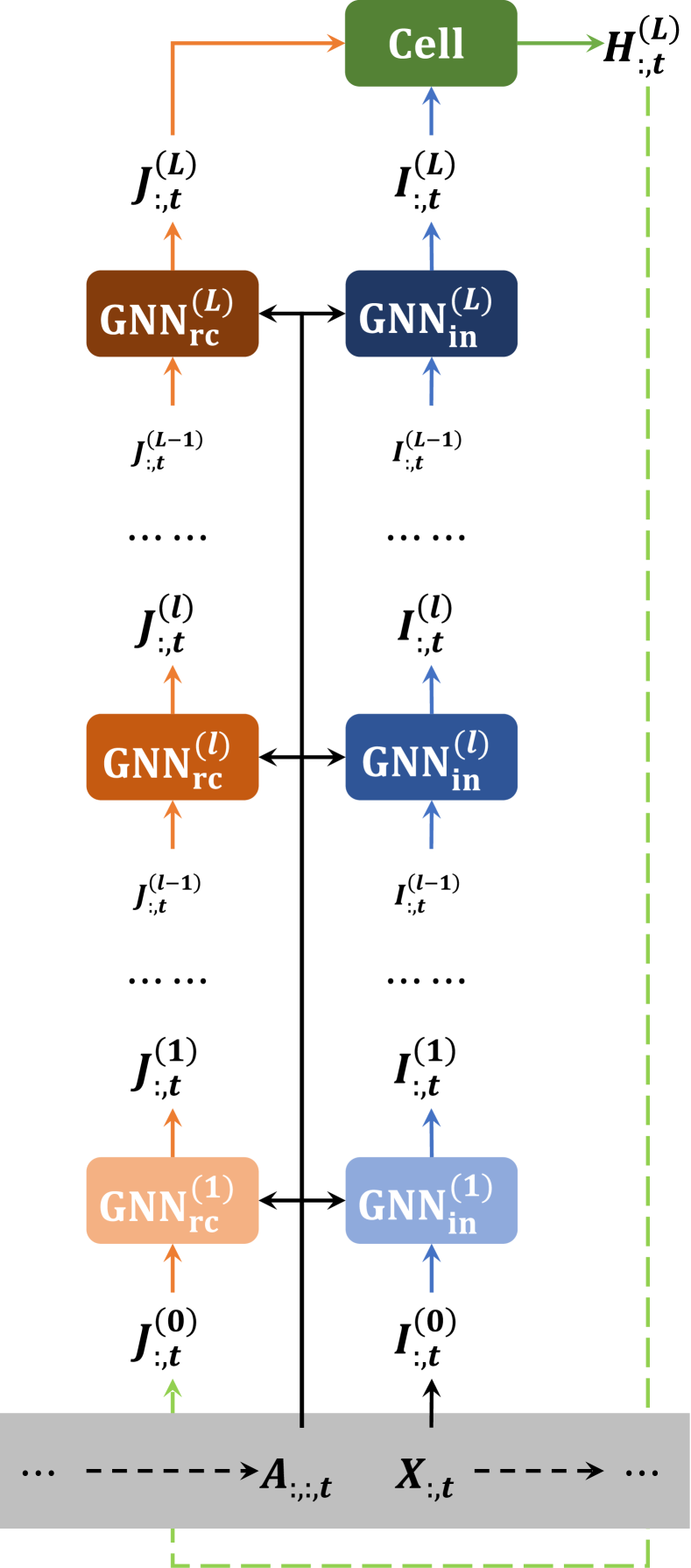
Figure 3: Illustration of a time-and-graph architecture: $\bm{\mathsf{X}}_{:,t}$ is all node attributes and $\bm{\mathsf{A}}_{:,:,t}$ is all edge attributes at snapshot $t$ for $1\leq t\leq T$. $\text{GNN}_{\text{in}}^{(l)}$ (blue) and $\text{GNN}_{\text{rc}}^{(l)}$ (orange) are $l$-th layer of $\text{GNN}_{\text{in}}^{L}$ and $\text{GNN}_{\text{rc}}^{L}$ as defined in Equation 5. Different color saturation means layer depth. Cell (green) is the RNN cell defined in Equation 5. $\bm{\mathsf{H}}_{:,t}$ is the historical representation output of time-and-graph until snapshot $t$, and $\bm{\mathsf{H}}_{:,T}$ will be the final representation output. $\bm{\mathsf{I}}_{:,t}^{(l)}$ is the internal (hidden) states of $\text{GNN}_{\text{in}}^{L}$ at layer $l$. $\bm{\mathsf{J}}_{:,t}^{(l)}$ is the internal (hidden) states of $\text{GNN}_{\text{rc}}^{L}$ at layer $l$.

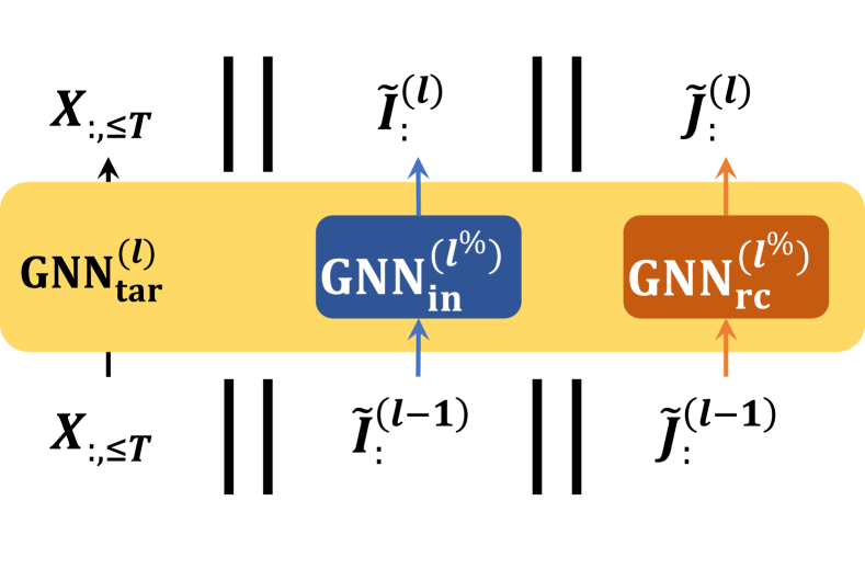
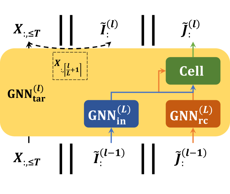
Figure 4: Illustration of $l$-th constructed time-then-graph layer in $\mathbf{\text{GNN}_{\text{tar}}^{TL}}$ when $\mathbf{l\text{ mod }L\neq 0}$: Yellow square is the illustration of Equations 12 and 13 when $t=\lceil l/L\rceil$. Operations (blue and orange squares) inside it imply the same operations as in Figure 5 with the same colors (regardless of saturation) and superscript values. We can see that for $l\text{ mod }L\neq 0$, any arbitrary layer $l$ of the $\text{GNN}_{\text{tar}}^{TL}$ is indeed processing layer $l^{\%}$ of $\text{GNN}_{\text{in}}^{L}$ and $\text{GNN}_{\text{rc}}^{L}$ at snapshot $t=\lceil l/L\rceil$ in parallel as Figure 5.

Figure 5: Illustration of $l$-th constructed time-then-graph layer in $\mathbf{\text{GNN}_{\text{tar}}^{TL}}$ when $\mathbf{l\text{ mod }L=0}$: Yellow square is the illustration of Equations 12 and 13 when $t=\lceil l/L\rceil$. Operations (green, blue and orange squares) inside it imply the same operations as in Figure 5 with the same colors (regardless of saturation) and superscript values. We can see that for $l\text{ mod }L=0$, different from the operations illustrated in the Figure 5, $\text{GNN}_{\text{tar}}^{(l)}$ will replace part of output, $\tilde{\bm{\mathsf{I}}}_{:}^{l}$, by node attributes $\bm{\mathsf{X}}_{:,\lceil l/L+1\rceil}$, and will replace the other part of output, $\tilde{\bm{\mathsf{J}}}_{:}^{l}$, by the output of Equation 10 which indeed is mirroring the operations after layer $L$ in Figure 5 (layer $L$ itself and recurrent cell).

First, we will show that any time-and-graph representation function has an equivalent time-then-graph function. We start with recalling the definition of time-and-graph given by Equation 5:

$$\bm{\mathsf{H}}_{i,t}=\text{Cell}\bigg{(}\Big{[}\text{GNN}_{\text{in}}^{L}\big{(}\bm{\mathsf{X}}_{:,t},\bm{\mathsf{A}}_{:,:,t}\big{)}\Big{]}_{i},\Big{[}\text{GNN}_{\text{rc}}^{L}\big{(}\bm{\mathsf{H}}_{:,t-1},\bm{\mathsf{A}}_{:,:,t}\big{)}\Big{]}_{i}\bigg{)}$$

The above definition has two different graph neural networks $\text{GNN}_{\text{in}}^{L}$ and $\text{GNN}_{\text{rc}}^{L}$. These represent encoding raw node attributes at time $t$ and encoding node historical representations before $t$ along with topology $\bm{\mathsf{A}}_{:,:,t}$ at snapshot $t$, respectively.

Also, we revisit the definition of GNN in Equation 1 of any arbitrary layer $l$ for the sake of later construction:

$$\bm{\mathsf{M}}_{i}^{(l)} =\sum\limits_{j\in\mathcal{N}(i)}\text{MSG}^{(l)}\big{(}\bm{\mathsf{Z}}_{i}^{(l-1)},\bm{\mathsf{Z}}_{j}^{(l-1)},\bm{\mathsf{A}}_{i,j}\big{)},$$

$$\bm{\mathsf{Z}}_{i}^{(l)} =\text{UPDATE}^{(l)}\big{(}\bm{\mathsf{Z}}_{i}^{(l-1)},\bm{\mathsf{M}}_{i}^{(l)}\big{)},$$

The full time-and-graph architecture is shown in Figure 5 and is formally described by 3 parts:

1. Description of $\text{GNN}_{\text{in}}^{L}$: This GNN embeds the input features at time $t\in\{1,\cdots,T\}$. To differentiate symbols from other GNN operations, we denote the $\text{GNN}_{\text{in}}^{(l)}$ definition at each layer $l\in\{1,\cdots,L\}$ as

   $$\bm{\mathsf{E}}_{i,t}^{(l)} =\sum\limits_{j\in\mathcal{N}_{t}(i)}\text{MSG}_{\text{in}}^{(l)}\big{(}\bm{\mathsf{I}}_{i,t}^{(l-1)},\bm{\mathsf{I}}_{j,t}^{(l-1)},\bm{\mathsf{A}}_{i,j,t}\big{)},$$ (8)

   $$\bm{\mathsf{I}}_{i,t}^{(l)} =\text{UPDATE}_{\text{in}}^{(l)}\big{(}\bm{\mathsf{I}}_{i,t}^{(l-1)},\bm{\mathsf{E}}_{i,t}^{(l)}\big{)},$$

   where $\bm{\mathsf{I}}_{i,t}^{(l)}$ represents the embedding of arbitrary node $i\in\mathcal{V}$ obtained at layer $l$ on snapshot $t$ and $\mathcal{N}_{t}(i)$ defines the neighbor set of $i$ on snapshot $t$. We also initialize the corner case $\bm{\mathsf{I}}_{i,t}^{(0)}=\bm{\mathsf{X}}_{i,t}$. $\text{MSG}_{\text{in}}^{(l)}$ and $\text{UPDATE}_{\text{in}}^{(l)}$ are learnable parametric functions of arbitrary forms, e.g., Multi-Layer Perceptions (MLPs). Finally, the output for arbitrary node $i\in\mathcal{V}$ is $\big{[}\text{GNN}_{\text{in}}^{L}\big{(}\bm{\mathsf{X}}_{:,t},\bm{\mathsf{A}}_{:,:,t}\big{)}\big{]}_{i}:=\bm{\mathsf{I}}_{i,t}^{(L)}$.

2. Description of $\text{GNN}_{\text{rc}}^{L}$: We denote the $\text{GNN}_{\text{rc}}^{(l)}$ definition at each layer $l\in\{1,\cdots,L\}$ as

   $$\bm{\mathsf{F}}_{i,t}^{(l)} =\sum\limits_{j\in\mathcal{N}_{t}(i)}\text{MSG}_{\text{rc}}^{(l)}\big{(}\bm{\mathsf{J}}_{i,t}^{(l-1)},\bm{\mathsf{J}}_{j,t}^{(l-1)},\bm{\mathsf{A}}_{i,j,t}\big{)},$$ (9)

   $$\bm{\mathsf{J}}_{i,t}^{(l)} =\text{UPDATE}_{\text{rc}}^{(l)}\big{(}\bm{\mathsf{J}}_{i,t}^{(l-1)},\bm{\mathsf{F}}_{i,t}^{(l)}\big{)},$$

   where $\bm{\mathsf{J}}_{i,t}^{(l)}$ represents the embedding of arbitrary node $i\in\mathcal{V}$ obtained at layer $l$ on snapshot $t$ and $\mathcal{N}_{t}(i)$ defines the neighbor set of $i$ on snapshot $t$. We also initialize the corner case $\bm{\mathsf{J}}_{i,t}^{(0)}=\bm{\mathsf{H}}_{i,t-1}$ ($\bm{\mathsf{H}}_{i,0}=0$ as defined later). $\text{MSG}_{\text{rc}}^{(l)}$ and $\text{UPDATE}_{\text{rc}}^{(l)}$ are learnable parametric functions of arbitrary forms, e.g., Multi-Layer Perceptions (MLPs). Finally, the output for arbitrary node $i\in\mathcal{V}$ is $\big{[}\text{GNN}_{\text{rc}}^{L}\big{(}\bm{\mathsf{H}}_{:,t-1},\bm{\mathsf{A}}_{:,:,t}\big{)}\big{]}_{i}:=\bm{\mathsf{J}}_{i,t}^{(L)}$.

3. Description of Cell: For the sake of simplicity, we redefine $\bm{\mathsf{H}}_{i,t}$ of Equation 5 based on aformentioned symbols:

   $$\bm{\mathsf{H}}_{i,t}=\text{Cell}\left(\bm{\mathsf{I}}_{i,t}^{(L)},\bm{\mathsf{J}}_{i,t}^{(L)}\right).$$ (10)

   We initialize the corner case $\bm{\mathsf{H}}_{i,0}=0$ for any node $i\in\mathcal{V}$.

Equations 8, 9 and 10 give a general description of existing architectures for time-and-graph representation functions. Finally, $\bm{\mathsf{H}}_{i,T}$ is the final temporal graph representation of node $i\in\mathcal{V}$, and is the target we want achieve from a constructed time-then-graph representation.

Now, our target is to construct a time-then-graph representation function, and we have to show the construction always give the same output $\bm{\mathsf{H}}_{i,T}$ for the same temporal graph input $\Big{(}\big{[}\bm{\mathsf{X}}_{i,t}\big{]}_{\forall i\in\mathcal{V},1\leq t\leq T},\big{[}\bm{\mathsf{A}}_{i,j,t}\big{]}_{\forall i,j\in\mathcal{V},1\leq t\leq T}\Big{)}$.

First, we revisit the definition of time-then-graph representation in Equation 7:

$$\bm{\mathsf{H}}^{\text{node}}_{i} =\text{RNN}^{\text{node}}\big{(}\bm{\mathsf{X}}_{i,\leq T}\big{)},\quad\forall i\in\mathcal{V},$$

$$\bm{\mathsf{H}}^{\text{edge}}_{i,j} =\text{RNN}^{\text{edge}}\big{(}\bm{\mathsf{A}}_{i,j,\leq T}\big{)},\quad\forall(i,j)\in\mathcal{E},$$

$$\bm{\mathsf{Z}} =\text{GNN}^{L}\big{(}\bm{\mathsf{H}}^{\text{node}},\bm{\mathsf{H}}^{\text{edge}}\big{)}.$$

Siegelmann & Sontag (1995) shows that with enough hidden neurons, a RNN can be a most-expressive sequence model (universal Turing machine approximator). Hence, since the representations for node and edge attribute sequences are most-expressive, we can equivalently think of those RNN outputs simply as “copy” of the inputs, i.e., $\bm{\mathsf{H}}^{\text{node}}_{i}$ perfectly represents $\bm{\mathsf{X}}_{i,\leq T}$ and $\bm{\mathsf{H}}^{\text{edge}}_{i,j}$ perfectly represents $\bm{\mathsf{A}}_{i,j,\leq T}$. Hence, for the ease of simplicity, we can construct time-then-graph representation just as a static GNN representation applied over the aggregated node attribute and adjacency matrix inputs:

$$\bm{\mathsf{Z}}^{\prime}=\text{GNN}_{\text{tar}}^{TL}\big{(}\bm{\mathsf{X}}_{:,\leq T},\bm{\mathsf{A}}_{:,:,\leq T}\big{)},$$

which we will describe construction details in the later content.

The constructed $\mathbf{\text{GNN}_{\text{tar}}^{TL}}$ representation details. The basic idea is straightforward: $\text{GNN}_{\text{tar}}^{TL}$ has $T\times L$ layers; Between layers $l\in\{(\tau-1)L+1,\cdots,\tau L\}$ of the construction, we will focus on emulating time-and-graph representation over node attributes $\bm{\mathsf{X}}_{:,\tau}$ and edges $\bm{\mathsf{A}}_{:,:,\tau}$ of snapshot $\tau=1,\cdots,T$, which is provided by the most-expressive sequence representations $\bm{\mathsf{X}}_{:,\leq T}$ and $\bm{\mathsf{A}}_{:,:,\leq T}$ as our construction input. In other words, constructed layer $l$ will work on data of snapshot $\lceil l/L\rceil$ where $L$ is the number of GNN layers in the simulating time-and-graph representation.

In what follows, we extend some notations for the ease of construction definition:

• $\|$ denotes a vector concatenation operator;

• $l^{\%}$ denotes for a modified modulo

  $$l^{\%}=\begin{cases}l\text{ mod }L,&l\text{ mod }L\neq 0,\\ L,&l\text{ mod }L=0;\end{cases}$$

• $\mathcal{N}(i)=\{\forall j\in\mathcal{V}|\exists\tau,1\leq\tau\leq T,\bm{\mathsf{A}}_{i,j,\tau}>0\}$ denotes the set of full neighbors of $i\in\mathcal{V}$ in the aggregated adjacency matrix over all $T$ times;

• $\mathcal{N}_{t}(i)$ is the neighbor set of node $i$ from $\bm{\mathsf{A}}_{:,:,t}$ at snapshot $t$.

Recall the time-and-graph definitions in Equations 8, 9 and 10, we subsitute their superscripts by $l^{\%}$ to fit our time-then-graph construction (e.g., $\text{MSG}_{\text{in}}^{(l^{\%})},\text{UPDATE}_{\text{in}}^{(l^{\%})},\text{MSG}_{\text{rc}}^{(l^{\%})},\text{UPDATE}_{\text{rc}}^{(l^{\%})}$). We further use a tilde symbol to corresponding output variables (e.g., $\bm{\mathsf{E}},\bm{\mathsf{I}},\bm{\mathsf{F}},\bm{\mathsf{J}}$) to reflect the simulating relationship in our construction (e.g., $\tilde{\bm{\mathsf{E}}},\tilde{\bm{\mathsf{I}}},\tilde{\bm{\mathsf{F}}},\tilde{\bm{\mathsf{J}}}$).

Then, we design the output of each constructed layer $l\in\{1,\cdots,TL\}$ as a combination of three parts $\big{[}\bm{\mathsf{X}}_{i,\leq T}\big{\|}\tilde{\bm{\mathsf{I}}}_{i}^{(l)}\big{\|}\tilde{\bm{\mathsf{J}}}_{i}^{(l)}\big{]}$ based on their usage

1. $\bm{\mathsf{X}}_{i,\leq T}$ is the attribute of node $i$ in aggregated temporal graph, and it can also be regarded as the concatenation of all attributes of node $i$ of all time steps $1\leq t\leq T$;

2. $\tilde{\bm{\mathsf{I}}}^{(l)}_{i},\tilde{\bm{\mathsf{J}}}^{(l)}_{j}$ is used to achieve the same representations as $\bm{\mathsf{I}}^{(l^{\%})}_{i,\lceil l/L\rceil},\bm{\mathsf{J}}^{(l^{\%})}_{j,\lceil l/L\rceil}$ in Equations 8 and 9.

For arbitrary node $i$ at constructon layer $l$, we need to constuct two essential GNN components $\text{MSG}_{\text{tar}}^{(l)}$ and $\text{UPDATE}_{\text{tar}}^{(l)}$ to properly pass these three parts as inputs and outputs. First, $\text{MSG}_{\text{tar}}^{(l)}$ takes the concatenation of three parts of arbitrary neighbor node $j\in\mathcal{N}(i)$ as input: Aggregated neighbor node attributes $\bm{\mathsf{X}}_{j,\leq T}$; And $\tilde{\bm{\mathsf{I}}}_{j}^{(l-1)},\tilde{\bm{\mathsf{J}}}_{j}^{(l-1)}$ that mimic $\bm{\mathsf{I}}^{(l^{\%}-1)}_{j,\lceil l/L\rceil},\bm{\mathsf{J}}^{(l^{\%}-1)}_{j,\lceil l/L\rceil}$ as in Equations 8 and 9. Then, $\text{UPDATE}_{\text{tar}}^{(l)}$ outputs $\big{[}\tilde{\bm{\mathsf{E}}}_{i}^{(l)}\big{\|}\tilde{\bm{\mathsf{F}}}_{i}^{(l)}\big{]}$ that mimic the representations of $\bm{\mathsf{E}}^{(l^{\%})}_{i,\lceil l/L\rceil},\bm{\mathsf{F}}^{(l^{\%})}_{i,\lceil l/L\rceil}$ as in Equations 8 and 9.

We also initialize the corner case

$$\big{[}\bm{\mathsf{X}}_{i,\leq T}\big{\|}\tilde{\bm{\mathsf{I}}}_{i}^{(0)}\big{\|}\tilde{\bm{\mathsf{J}}}_{i}^{(0)}\big{]}=\big{[}\bm{\mathsf{X}}_{i,\leq T}\big{\|}\bm{\mathsf{X}}_{i,1}\big{\|}0\big{]},$$ (11)

for any node $i$.

In the following Equations 12 and 13 we give formal constructions of functions $\mathbf{\text{MSG}_{\text{tar}}^{(l)}}$ and $\mathbf{\text{UPDATE}_{\text{tar}}^{(l)}}$ in $\mathbf{\text{GNN}_{\text{tar}}^{TL}}$ so that they can mimic all variables as discussed before:

$$\sum\limits_{j\in\mathcal{N}(i)}\text{MSG}_{\text{tar}}^{(l)}\big{(}\big{[}\bm{\mathsf{X}}_{i,\leq T}\big{\|}\tilde{\bm{\mathsf{I}}}_{i}^{(l-1)}\big{\|}\tilde{\bm{\mathsf{J}}}_{i}^{(l-1)}\big{]},\big{[}\bm{\mathsf{X}}_{j,\leq T}\big{\|}\tilde{\bm{\mathsf{I}}}_{j}^{(l-1)}\big{\|}\tilde{\bm{\mathsf{J}}}_{j}^{(l-1)}\big{]},\bm{\mathsf{A}}_{i,j,\leq T}\big{)}$$ (12)

$$=\Bigg{[}\sum\limits_{j\in\mathcal{N}_{\lceil\frac{l}{L}\rceil}(i)}\text{MSG}_{\text{in}}^{(l^{\%})}\big{(}\tilde{\bm{\mathsf{I}}}_{i}^{(l-1)},\tilde{\bm{\mathsf{I}}}_{j}^{(l-1)},\bm{\mathsf{A}}_{i,j,\lceil\frac{l}{L}\rceil}\big{)}\Bigg{\|}\sum\limits_{j\in\mathcal{N}_{\lceil\frac{l}{L}\rceil}(i)}\text{MSG}_{\text{rc}}^{(l^{\%})}\big{(}\tilde{\bm{\mathsf{J}}}_{i}^{(l-1)},\tilde{\bm{\mathsf{J}}}_{j}^{(l-1)},\bm{\mathsf{A}}_{i,j,\lceil\frac{l}{L}\rceil}\big{)}\Bigg{]}$$

$$=\big{[}\tilde{\bm{\mathsf{E}}}_{i}^{(l)}\big{\|}\tilde{\bm{\mathsf{F}}}_{i}^{(l)}\big{]}.$$

$$\text{UPDATE}_{\text{tar}}^{(l)}\big{(}\big{[}\bm{\mathsf{X}}_{i,\leq T}\big{\|}\tilde{\bm{\mathsf{I}}}_{i}^{(l-1)}\big{\|}\tilde{\bm{\mathsf{J}}}_{i}^{(l-1)}\big{]},\big{[}\tilde{\bm{\mathsf{E}}}_{i}^{(l)}\big{\|}\tilde{\bm{\mathsf{F}}}_{i}^{(l)}\big{]}\big{)}$$ (13)

$$=\begin{dcases}\Big{[}\bm{\mathsf{X}}_{i,\leq T}\Big{\|}\text{UPDATE}_{\text{in}}^{(l^{\%})}\big{(}\tilde{\bm{\mathsf{I}}}_{i}^{(l-1)},\tilde{\bm{\mathsf{E}}}_{i}^{(l)}\big{)}\Big{\|}\text{UPDATE}_{\text{rc}}^{(l^{\%})}\big{(}\tilde{\bm{\mathsf{J}}}_{i}^{(l-1)},\tilde{\bm{\mathsf{F}}}_{i}^{(l)}\big{)}\Big{]},&l\text{ mod }L\neq 0,\\ \bigg{[}\bm{\mathsf{X}}_{i,\leq T}\bigg{\|}\bm{\mathsf{X}}_{i,\lceil\frac{l}{L}+1\rceil}\bigg{\|}\text{Cell}\Big{(}\text{UPDATE}_{\text{in}}^{(l^{\%})}\big{(}\tilde{\bm{\mathsf{I}}}_{i}^{(l-1)},\tilde{\bm{\mathsf{E}}}_{i}^{(l)}\big{)},\text{UPDATE}_{\text{rc}}^{(l^{\%})}\big{(}\tilde{\bm{\mathsf{J}}}_{i}^{(l-1)},\tilde{\bm{\mathsf{F}}}_{i}^{(l)}\big{)}\Big{)}\bigg{]},&l\text{ mod }L=0,\end{dcases}$$

$$=\big{[}\bm{\mathsf{X}}_{i,\leq T}\big{\|}\tilde{\bm{\mathsf{I}}}_{i}^{(l)}\big{\|}\tilde{\bm{\mathsf{J}}}_{i}^{(l)}\big{]}.$$

Finally, we are going to show the GNN construction defined by Equations 12 and 13 can give the same output $\mathbf{\bm{\mathsf{H}}_{i,T}}$ as in Equation 8 for all nodes $\mathbf{i\in\mathcal{V}}$. Indeed, we will show by induction that $\tilde{\bm{\mathsf{J}}}_{i}^{(tL)}=\bm{\mathsf{H}}_{i,t}$ for arbitrary node $i$ at any time $t\in\{0,\cdots,T\}$.

First, as the initial point of induction, for any node $i\in V$ before the first layer $l\leftarrow 1$, based on Equation 11, we initialize the input by

$$\big{[}\bm{\mathsf{X}}_{i,\leq T}\big{\|}\tilde{\bm{\mathsf{I}}}_{i}^{(0)}\big{\|}\tilde{\bm{\mathsf{J}}}_{i}^{(0)}\big{]}=\big{[}\bm{\mathsf{X}}_{i,\leq T}\big{\|}\bm{\mathsf{X}}_{i,1}\big{\|}0\big{]}.$$

This implies that

$$\tilde{\bm{\mathsf{I}}}_{i}^{(0)} =\bm{\mathsf{X}}_{i,1}=\bm{\mathsf{I}}_{i,1}^{(0)},\quad\forall i\in\mathcal{V},$$

$$\tilde{\bm{\mathsf{J}}}_{i}^{(0)} =0=\bm{\mathsf{J}}_{i,1}^{(0)}=\bm{\mathsf{H}}_{i,0},\quad\forall i\in\mathcal{V}.$$

Thus, $\tilde{\bm{\mathsf{J}}}_{i}^{(tL)}=\bm{\mathsf{H}}_{i,t}$ holds when $t\leftarrow 0$.

Now, suppose that

$$\tilde{\bm{\mathsf{I}}}_{i}^{(l-1)} =\bm{\mathsf{I}}_{i,\lceil\frac{l}{L}\rceil}^{(l^{\%}-1)},\quad\forall i\in\mathcal{V},$$ (14)

$$\tilde{\bm{\mathsf{J}}}_{i}^{(l-1)} =\bm{\mathsf{J}}_{i,\lceil\frac{l}{L}\rceil}^{(l^{\%}-1)},\quad\forall i\in\mathcal{V},$$

for arbitrary $l\in\{1,\cdots,TL\}$.

Next, as the first step of induction, we show the message outputs of Equation 12 is the same as message outputs of Equations 8 and 9 given the condition in Equation 14.

$$\tilde{\bm{\mathsf{E}}}_{i}^{(l)} =\sum\limits_{j\in\mathcal{N}_{\lceil\frac{l}{L}\rceil}(i)}\text{MSG}_{\text{in}}^{(l^{\%})}\big{(}\tilde{\bm{\mathsf{I}}}_{i}^{(l-1)},\tilde{\bm{\mathsf{I}}}_{j}^{(l-1)},\bm{\mathsf{A}}_{i,j,\lceil\frac{l}{L}\rceil}\big{)}$$ (15)

$$=\sum\limits_{j\in\mathcal{N}_{\lceil\frac{l}{L}\rceil}(i)}\text{MSG}_{\text{in}}^{(l^{\%})}\big{(}\bm{\mathsf{I}}_{i,\lceil\frac{l}{L}\rceil}^{(l^{\%}-1)},\bm{\mathsf{I}}_{j,\lceil\frac{l}{L}\rceil}^{(l^{\%}-1)},\bm{\mathsf{A}}_{i,j,\lceil\frac{l}{L}\rceil}\big{)}$$

$$=\bm{\mathsf{E}}_{i,\lceil\frac{l}{L}\rceil}^{(l^{\%})},$$

$$\tilde{\bm{\mathsf{F}}}_{i}^{(l)} =\sum\limits_{j\in\mathcal{N}_{\lceil\frac{l}{L}\rceil}(i)}\text{MSG}_{\text{rc}}^{(l^{\%})}\big{(}\tilde{\bm{\mathsf{J}}}_{i}^{(l-1)},\tilde{\bm{\mathsf{J}}}_{j}^{(l-1)},\bm{\mathsf{A}}_{i,j,\lceil\frac{l}{L}\rceil}\big{)}$$

$$=\sum\limits_{j\in\mathcal{N}_{\lceil\frac{l}{L}\rceil}(i)}\text{MSG}_{\text{rc}}^{(l^{\%})}\big{(}\bm{\mathsf{J}}_{i,\lceil\frac{l}{L}\rceil}^{(l^{\%}-1)},\bm{\mathsf{J}}_{j,\lceil\frac{l}{L}\rceil}^{(l^{\%}-1)},\bm{\mathsf{A}}_{i,j,\lceil\frac{l}{L}\rceil}\big{)}$$

$$=\bm{\mathsf{F}}_{i,\lceil\frac{l}{L}\rceil}^{(l^{\%})}.$$

Then, as the second step of induction, we show the update outputs of Equation 13 is the same as update outputs of Equations 8 and 9 given the condition in Equation 14 and Equation 15. Pay attention that there are two cases in Equation 13, and we will show those cases one by one.

When $l\text{ mod }L\neq 0$,

$$\tilde{\bm{\mathsf{I}}}_{i}^{(l)} =\text{UPDATE}_{\text{in}}^{(l^{\%})}\big{(}\tilde{\bm{\mathsf{I}}}_{i}^{(l-1)},\tilde{\bm{\mathsf{E}}}_{i}^{(l)}\big{)}$$ (16)

$$=\text{UPDATE}_{\text{in}}^{(l^{\%})}\big{(}\bm{\mathsf{I}}_{i,\lceil\frac{l}{L}\rceil}^{(l^{\%}-1)},\bm{\mathsf{E}}_{i,\lceil\frac{l}{L}\rceil}^{(l^{\%})}\big{)}$$

$$=\bm{\mathsf{I}}_{i,\lceil\frac{l}{L}\rceil}^{(l^{\%})}=\bm{\mathsf{I}}_{i,\lceil\frac{l+1}{L}\rceil}^{(l^{\%})},$$

$$\tilde{\bm{\mathsf{J}}}_{i}^{(l)} =\text{UPDATE}_{\text{rc}}^{(l^{\%})}\big{(}\tilde{\bm{\mathsf{J}}}_{i}^{(l-1)},\tilde{\bm{\mathsf{F}}}_{i}^{(l)}\big{)}$$

$$=\text{UPDATE}_{\text{rc}}^{(l^{\%})}\big{(}\bm{\mathsf{J}}_{i,\lceil\frac{l}{L}\rceil}^{(l^{\%}-1)},\bm{\mathsf{F}}_{i,\lceil\frac{l}{L}\rceil}^{(l^{\%})}\big{)}$$

$$=\bm{\mathsf{J}}_{i,\lceil\frac{l}{L}\rceil}^{(l^{\%})}=\bm{\mathsf{J}}_{i,\lceil\frac{l+1}{L}\rceil}^{(l^{\%})}.$$

We can see that Equation 16 are indeed Equation 14 when $l\leftarrow l+1$. We provide a sketched illustration for this induction case in Figure 5.

When $l\text{ mod }L=0$,

$$\tilde{\bm{\mathsf{I}}}_{i}^{(l)} =\bm{\mathsf{X}}_{i,\lceil\frac{l}{L}+1\rceil}=\bm{\mathsf{I}}_{i,\lceil\frac{l+1}{L}\rceil}^{(0)},$$ (17)

$$\tilde{\bm{\mathsf{J}}}_{i}^{(l)} =\text{Cell}\big{(}\text{UPDATE}_{\text{in}}^{(l^{\%})}\big{(}\tilde{\bm{\mathsf{I}}}_{i}^{(l-1)},\tilde{\bm{\mathsf{E}}}_{i}^{(l)}\big{)},\text{UPDATE}_{\text{rc}}^{(l^{\%})}\big{(}\tilde{\bm{\mathsf{J}}}_{i}^{(l-1)},\tilde{\bm{\mathsf{F}}}_{i}^{(l)}\big{)}\big{)}$$

$$=\text{Cell}\big{(}\text{UPDATE}_{\text{in}}^{(l^{\%})}\big{(}\bm{\mathsf{I}}_{i,\lceil\frac{l}{L}\rceil}^{(l^{\%}-1)},\bm{\mathsf{E}}_{i,\lceil\frac{l}{L}\rceil}^{(l^{\%})}\big{)},\text{UPDATE}_{\text{rc}}^{(l^{\%})}\big{(}\bm{\mathsf{J}}_{i,\lceil\frac{l}{L}\rceil}^{(l^{\%}-1)},\bm{\mathsf{F}}_{i,\lceil\frac{l}{L}\rceil}^{(l^{\%})}\big{)}\big{)}$$

$$=\text{Cell}\big{(}\bm{\mathsf{I}}_{i,\lceil\frac{l}{L}\rceil}^{(L)},\bm{\mathsf{J}}_{i,\lceil\frac{l}{L}\rceil}^{(L)}\big{)}$$

$$=\bm{\mathsf{H}}_{i,\lceil\frac{l}{L}\rceil}=\bm{\mathsf{J}}_{i,\lceil\frac{l+1}{L}\rceil}^{(0)}.$$

We can see that Equation 17 also corresponds to Equation 14 when $l\leftarrow l+1$. We provide a sketched illustration for this induction case in Figure 5.

We continue the induction until layer $l\leftarrow TL$, where we stop, and Equation 17 eventually yields

$$\tilde{\bm{\mathsf{J}}}_{i}^{(TL)}=\bm{\mathsf{H}}_{i,T}.$$

This implies that we get the targeting time-and-graph representation output $\bm{\mathsf{H}}_{i,T}$ from constructed (static) GNN output for an arbitrary node $i\in\mathcal{V}$.

The above shows that any arbitrary time-and-graph representation relying on 1-WL GNNs (Equations 8, 9 and 10) can be emulated by a time-then-graph representation (Equations 12 and 13), which outputs the same representations for the same temporal graph inputs. Thus, time-then-1WLGNN is at least the same expressive as time-and-1WLGNN based on Lemma 3.4.

Finally, we show a specific task (illustrated as Figure 2) where time-then-1WLGNN is more expressive than time-and-1WLGNN.

We now propose a synthetic task, whose temporal graph is illustrated in Figure 2. The goal is to differentiate the topologies between two 2-step temporal graphs. Each snapshot is a Circular Skip Link (CSL) graph (see Murphy et al. (2019)) with 7 unattributed nodes, denoted as $\mathcal{C}_{7,s}$, where $s$ represents the smallest number of nodes on the outer circle between two neighbors which are not connected by the outer circle. For example, “a” and “c” are such two neighbors in $\mathcal{C}_{7,1}$, and the nodes on the outer circle between them is “b”, which means $s=1$.

In Figure 2, two temporal graphs differ in their second time step $t_{2}$. From (Murphy et al., 2019), if the CSL graphs are unattributed, any 1-WL GNN will output the same representations for both $\mathcal{C}_{7,1}$ and $\mathcal{C}_{7,2}$. We use $\bm{\mathsf{A}}^{(\text{top})}$ to represent the adjacency matrix of dynamics in the top left of Figure 2, and $\bm{\mathsf{A}}^{(\text{btm})}$ for dynamics in the bottom left of Figure 2. Note that $\bm{\mathsf{X}}^{(\text{top})}=\bm{\mathsf{X}}^{(\text{btm})}=0$ since the temporal graph is unattributed.

Hence, for a time-and-1WLGNN representation,

$$\text{GNN}_{\text{in}}^{L}\big{(}\bm{\mathsf{X}}^{(\text{top})}_{:,1},\bm{\mathsf{A}}^{(\text{top})}_{:,:,1}\big{)}=\text{GNN}_{\text{in}}^{L}\big{(}\bm{\mathsf{X}}^{(\text{top})}_{:,2},\bm{\mathsf{A}}^{(\text{top})}_{:,:,2}\big{)}=\text{GNN}_{\text{in}}^{L}\big{(}\bm{\mathsf{X}}^{(\text{btm})}_{:,1},\bm{\mathsf{A}}^{(\text{btm})}_{:,:,1}\big{)}=\text{GNN}_{\text{in}}^{L}\big{(}\bm{\mathsf{X}}^{(\text{btm})}_{:,2},\bm{\mathsf{A}}^{(\text{btm})}_{:,:,2}\big{)},$$

$$\text{GNN}_{\text{rc}}^{L}\big{(}\bm{\mathsf{H}}^{(\text{top})}_{:,0},\bm{\mathsf{A}}^{(\text{top})}_{:,:,1}\big{)}=\text{GNN}_{\text{rc}}^{L}\big{(}0,\bm{\mathsf{A}}^{(\text{top})}_{:,:,1}\big{)}=\text{GNN}_{\text{rc}}^{L}\big{(}\bm{\mathsf{H}}^{(\text{btm})}_{:,0},\bm{\mathsf{A}}^{(\text{btm})}_{:,:,1}\big{)}=\text{GNN}_{\text{rc}}^{L}\big{(}0,\bm{\mathsf{A}}^{(\text{btm})}_{:,:,1}\big{)}.$$

Then, when we apply Equation 10 at the first time step, we will get exactly the same hidden representation $\bm{\mathsf{H}}^{(\text{top})}_{:,1}$ and $\bm{\mathsf{H}}^{(\text{btm})}_{:,1}$. This also results in exactly the same hidden representation $\bm{\mathsf{H}}^{(\text{top})}_{:,2}$ and $\bm{\mathsf{H}}^{(\text{btm})}_{:,2}$ following similar computations. Thus, time-and-1WLGNN will output the same final representation $\mathbf{\bm{\mathsf{H}}^{(\text{top})}_{:,2}}$ and $\mathbf{\bm{\mathsf{H}}^{(\text{btm})}_{:,2}}$ for two different temporal graphs in Figure 2.

On the other hand, time-then-1WLGNN will work directly on aggregated graph as shown in the right side of Figure 2. Here, we can manually verify that a 1-WL GNN can distinguish these two aggregated graphs, implying that a time-then-1WLGNN representation can distinguish these two temporal graphs that time-and-1WLGNN cannot distinguish.

Finally, we conclude:

1. The time-then-1WLGNN is at least as expressive as the time-and-1WLGNN;

2. The time-then-1WLGNN can distinguish temporal graphs not distinguishable by time-and-1WLGNN.

Thus, time-then-1WLGNN is strictly more expressive than time-and-1WLGNN. More precisely,

$$\text{{{\em Time-and-1WLGNN}}}\precneqq_{\mathbb{T}^{|\mathcal{V}|,T,p}}\text{{{\em Time-then-1WLGNN}}},$$

concluding our proof.

Besides, we show that graph-then-time is a strict subset of time-and-graph by definition (Equations 6 and 5), thus it is straightforward that time-and-1WLGNN is strictly more expressive than 1WLGNN-then-time.

∎

A.3 Temporal GNN Expressivity

See 3.6

Proof.

In the proof of Theorem 3.5, we have noted that we can think the RNNs of time-then-graph as capable of perfectly copying the sequence into a representation, which ensures that the time-then-graph expressivity is equivalent to the expressivity of a (static) GNN whose node and edge attributes are their respective temporal sequences.

In Morris et al. (2019), it is shown that $\text{1-WL GNN}\precneqq_{\mathbb{G}_{|\mathcal{V}|,p}}\text{$k$-WL GNN}$. And Murphy et al. (2019); Maron et al. (2019a) both define most expressive graph representations which we denote as GNN⁺.

Using these known RNN and GNN expressivity results we have

$$\text{1-WL GNN}\precneqq_{\mathbb{G}^{|\mathcal{V}|,p}}\text{$k$-WL GNN}\precneqq_{\mathbb{G}^{|\mathcal{V}|,p}}\text{GNN${}^{+}$}$$

respectively, which then yields

$$\text{{\em time-then-1WLGNN}}\precneqq_{\mathbb{T}^{|\mathcal{V}|,T,p}}\text{{\em time-then-$k$WLGNN}}\precneqq_{\mathbb{T}^{|\mathcal{V}|,T,p}}\text{{\em time-then-GNN${}^{+}$}}$$

and time-then-GNN⁺ is the most expressive representation on $\mathbb{T}_{|\mathcal{V}|,T,p}$.

On the other hand, if we have the most expressive graph representation GNN⁺, then we can have an injection from any non-isomorphic snapshots to unique representations. Since RNN is also the most expressive for finite-length sequences, there also exists an injection from finite-length sequence of snapshot representations to a final time-and-GNN⁺ representation. Combining these two injections together, we can always get a representation injection from temporal graph space $\mathbb{T}_{|\mathcal{V}|,T,p}$, thus time-and-GNN⁺ is also the most expressive representation on $\mathbb{T}_{|\mathcal{V}|,T,p}$. Hence, both time-then-GNN⁺ and time-and-GNN⁺ are most-expressive representations of temporal attributed graphs with discrete time steps.

To summarize, we eventually have

$$\text{{\em time-then-1WLGNN}}\precneqq_{\mathbb{T}_{|\mathcal{V}|,T,p}}\text{{\em time-then-$k$WLGNN}}\precneqq_{\mathbb{T}_{|\mathcal{V}|,T,p}}\text{{\em time-then-GNN${}^{+}$}}\stackrel{{\scriptstyle e}}{{=}}_{\mathbb{T}_{|\mathcal{V}|,T,p}}\text{{\em time-and-GNN${}^{+}$}}.$$

∎

A.4 TGAT and TGN Failiure on DynCSL

Interestingly, TGAT and TGN, as a subset of time-then-graph representation (but not time-and-graph) baselines, they still do not work in the synthetic DynCSL task just as time-and-graph baselines (see Table 2). This poor performance is caused by the heterogeneous graph construction in TGAT and TGN. We will take TGN on Figure 2 for the case study, and TGAT will follow similar explanation.

The first step of TGN is collecting all edges connecting to the same node over all times as a sequence, and update temporal node attributes by the representation of the collected sequence. In two temporal graphs of Figure 2, all nodes are unattributed and their 1-hop topologies are always the same at every snapshot. Take node “a” in the top temporal graph as an example.

1. At the first step $t_{1}$, we will have its 1-hop topologies over all time as

   $$\Big{[}\big{(}\bm{\mathsf{X}}_{\text{b},1},\bm{\mathsf{A}}_{\text{a},\text{b},1},t_{1}\big{)},\big{(}\bm{\mathsf{X}}_{\text{c},1},\bm{\mathsf{A}}_{\text{a},\text{c},1},t_{1}\big{)},\big{(}\bm{\mathsf{X}}_{\text{f},1},\bm{\mathsf{A}}_{\text{a},\text{f},1},t_{1}\big{)},\big{(}\bm{\mathsf{X}}_{\text{g},1},\bm{\mathsf{A}}_{\text{a},\text{g},1},t_{1}\big{)}\Big{]}.$$

   Since temporal graphs are unattributed, we can simply regard this as a sequence of 4 same elements $t_{1}$. Suppose the representation of this sequence is $h_{1}$.

2. At the second step $t_{2}$, we will have its 1-hop topologies over all time as

   $$\Big{[} \big{(}\bm{\mathsf{X}}_{\text{b},1},\bm{\mathsf{A}}_{\text{a},\text{b},1},t_{1}\big{)},\big{(}\bm{\mathsf{X}}_{\text{c},1},\bm{\mathsf{A}}_{\text{a},\text{c},1},t_{1}\big{)},\big{(}\bm{\mathsf{X}}_{\text{f},1},\bm{\mathsf{A}}_{\text{a},\text{f},1},t_{1}\big{)},\big{(}\bm{\mathsf{X}}_{\text{g},1},\bm{\mathsf{A}}_{\text{a},\text{g},1},t_{1}\big{)},$$

   $$\big{(}\bm{\mathsf{X}}_{\text{b},2},\bm{\mathsf{A}}_{\text{a},\text{b},2},t_{2}\big{)},\big{(}\bm{\mathsf{X}}_{\text{c},2},\bm{\mathsf{A}}_{\text{a},\text{c},2},t_{2}\big{)},\big{(}\bm{\mathsf{X}}_{\text{f},2},\bm{\mathsf{A}}_{\text{a},\text{f},2},t_{2}\big{)},\big{(}\bm{\mathsf{X}}_{\text{g},2},\bm{\mathsf{A}}_{\text{a},\text{g},2},t_{2}\big{)}\Big{]}.$$

   Since temporal graphs are unattributed, we can simply regard this as a sequence of 4 elements $t_{1}$ and 4 elements $t_{2}$. Suppose the representation of this sequence is $h_{2}$.

Since all nodes have the same topologies, thus the newly constructed node attributes are only different between different times, and are the same for nodes at the same snapshot.

Next, TGN will get GNN representation from heterogeneous graph constructed by above node attributes $h_{1}$ and $h_{2}$. We still take node “a” as the example. The neighbor set of “a” in the heterogeneous graph will be

$$\Big{\{}\!\!\Big{\{} \big{(}h_{1},\bm{\mathsf{A}}_{\text{a},\text{b},1},t_{1}\big{)},\big{(}h_{1},\bm{\mathsf{A}}_{\text{a},\text{c},1},t_{1}\big{)},\big{(}h_{1},\bm{\mathsf{A}}_{\text{a},\text{f},1},t_{1}\big{)},\big{(}h_{1},\bm{\mathsf{A}}_{\text{a},\text{g},1},t_{1}\big{)},$$

$$\big{(}h_{2},\bm{\mathsf{A}}_{\text{a},\text{b},2},t_{2}\big{)},\big{(}h_{2},\bm{\mathsf{A}}_{\text{a},\text{c},2},t_{2}\big{)},\big{(}h_{2},\bm{\mathsf{A}}_{\text{a},\text{f},2},t_{2}\big{)},\big{(}h_{2},\bm{\mathsf{A}}_{\text{a},\text{g},2},t_{2}\big{)}\Big{\}}\!\!\Big{\}}.$$

Since temporal graphs are unattributed, this is indeed a multiset of 4 tuples $(h_{1},t_{1})$ and 4 tuples $(h_{2},t_{2})$. We can simply repeat this process on the bottom temporal graph, and can easily find node “a” in the bottom temporal graph will eventually get the same multiset. When the neighbor multisets are the same, 1-WL GNN will always return the same representations. Thus, there is no way to differeniate these two temporal graphs by TGN.

This case study explains the poor performance of TGAT and TGN on DynCSL dataset.

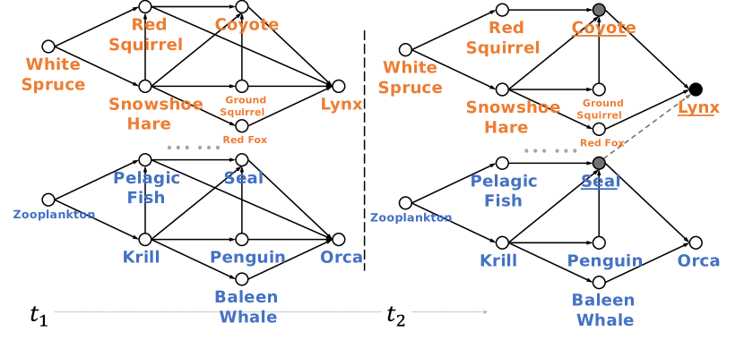
Figure 6: Equivariant expressivity insufficiency instance for temporal graph. A simple example of two disconnected components on a temporal knowledge graph without attributes, boreal forest (orange) and antarctic fauna (blue) over two-time dynamics in a food chain system. The two disconnected components have the same dynamics because of similar prey and predator environments in the isolated ecosystems. Extending Srinivasan & Ribeiro (2020) to temporal graphs, we can show that equivariant node representations of both time-then-graph and time-and-graph will output the same temporal representations for solid gray nodes “Coyote” and “Seal” for the same temporal structure at $t_{2}$. Hence, temporal link prediction based on these node representations will predict the same predator-prey edges, e.g., with solid black “Lynx”, where predicted dash edge between “Seal” and “Lynx” (which implies lynx also eat seal) is false positive.

A.5 Expressivity Insufficency For Link Prediction

In this subsection, we give more details about the expressivity insufficiency introduced in Section 5. We focus the expressivity study mostly on time-then-graph, since we have shown that time-then-graph is at least of the same expressvity as time-and-graph as Theorem 3.5 and Theorem 3.6 with any kinds of GNNs. We start with the statement that an equivariant graph representation is a structural node representation, since a permutation acts on the nodes (refer You et al. (2019); Srinivasan & Ribeiro (2020) for a description of the difference between structural and positional node representations).

Figure 6 shows a temporal graph with two disconnected components (orange and blue) in a food web with two isolated ecosystems. At each time step, the two disconnected components have the same topology. Then, the sequences of snapshots of the aggregated temporal graphs will be the same in these two disconnected components. This means that the time-then-graph aggregated forms of the two disconnected components (forest and sea) are exactly the same at time $t_{2}$. We can now invoke (Srinivasan & Ribeiro, 2020) for static attributed graphs to declare that the “Coyote” and “Seal” will receive the same time-then-graph most expressive and equivariant node representation at time $t_{2}$. By Theorem 3.6, the most expressive time-then-graph representation is as expressive as the most expressive time-and-graph representation, thus “Coyote” and “Seal” will also have the same time-and-graph equivariant node representation.

Since “Coyote” and “Seal” have the same temporal node representations, the method will incorrectly predict predatory links between two isolated ecosystem. For instance, if we want to predict their relationship with “Lynx”, node representation based methods will predict both/none of “Coyote” and “Seal” have link to “Lynx” at second step. The true answer is that “Coyote” has link to “Lynx” (directly shown in Figure 6 observation), but “Seal” should have no link to “Lynx” (in two isolated ecosystems). So, the prediction based on such equivariant node representations will always give wrong prediction at least for one animal kind. Thus, equvariant time-and-graph and time-then-graph temporal node representations are insufficiently expressive to predict temporal links.

Appendix B Experiment Configurations

Table 5: Model Designs. We introduce model architecture details in this table. Representation corresponds to the temporal graph representation families introduced in Section 2. Node RNN corresponds to the sequence representation applies on node-level data. Edge RNN corresponds to the sequence representation applies on edge-level data. GNN corresponds to the graph representation applies on graph data (either snapshots or aggregation). Other corresponds to implementation details which can not be simply clarified in this table, and is explained in Section B.1.

Model	Representation	Node RNN	Edge RNN	GNN	Other
EvolveGCN-O	graph-then-time	LSTM (Hochreiter & Schmidhuber, 1997)	N/A	GCN (Kipf & Welling, 2016)	Recurrent${}_{\text{O}}$ Weight
EvolveGCN-H		GRU (Chung et al., 2014)	N/A	GCN (Kipf & Welling, 2016)	Recurrent${}_{\text{H}}$ Weight
GCN-GRU		GRU (Chung et al., 2014)	N/A	GCN (Kipf & Welling, 2016)
DySAT		GAT (Veličković et al., 2018)	N/A	Attn (Vaswani et al., 2017)
GCRN-M2	time-and-graph	LSTM (Hochreiter & Schmidhuber, 1997)	N/A	Spectral (Defferrard et al., 2016)
DCRNN		GRU (Chung et al., 2014)	N/A	Spectral (Defferrard et al., 2016)	Concatenate
TGAT	time-then-graph	N/A	Heterogeneous	GAT (Veličković et al., 2018)	Relative
TGN		Last	Heterogeneous	GAT (Veličković et al., 2018)	Incremental
GRU-GCN		GRU (Chung et al., 2014)	GRU (Chung et al., 2014)	GCN (Kipf & Welling, 2016)	Skip

B.1 Our Model and Baselines

We summarize all architectures of our model and baselines in Table 5. It covers most of the details of architecture designs. However, there are still some implementation details which can not be simply explained in Table 5. We will briefly introduce those implementation details in later paragraphs.

Recurrent Weight. In both EvolveGCN-O and EvolveGCN-H, the hidden variable of RNNs is the weight paremeters of their GNNs rather than the representations of history snapshots. Thus, RNN will model the evolution of GNN parameters, rather than snapshot attributes. At each snapshot, GNN is initialized by parameters given by RNNs, and only receives current node and edge attributes as inputs to get final representations. The difference between EvolveGCN-O and EvolveGCN-H is that RNN of EvolveGCN-O recurrently outputs GNN parameters without receiving any inputs, while RNN of EvolveGCN-H takes node attributes $\bm{\mathsf{X}}_{:,t}$ as inputs and models parameter evolution with respect to node attributes. We use different subscripts in Table 5 to distinguish the RNN difference between two models.

Concatenate. In DCRNN, instead of apply two GNNs independently on $\big{(}\bm{\mathsf{X}}_{:,t},\bm{\mathsf{A}}_{:,:,t}\big{)}$ and $\big{(}\bm{\mathsf{H}}_{:,t-1},\bm{\mathsf{A}}_{:,:,t}\big{)}$ as Equation 5, it first concatenates $\bm{\mathsf{X}}_{:,t}$ and $\bm{\mathsf{H}}_{:,t-1}$ of the same nodes together as new node attributes, then get GNN representations on the snapshot with concatentated node attributes and edge attributes $\bm{\mathsf{A}}_{:,:,t}$ as RNN outputs $\bm{\mathsf{H}}_{:,t}$.

Heterogeneous. In both TGAT and TGN, it will collect all the edges connected to the same nodes together and construct a heterogeneous graph for GNNs to embed. For example, suppose for node $1$ we have following edges and neighbors over time: Edge $\bm{\mathsf{A}}_{1,2,1}$ from node $2$ at time $t_{1}$, $\bm{\mathsf{A}}_{1,3,1}$ from node $3$ at time $t_{1}$, and edge $\bm{\mathsf{A}}_{1,3,2}$ from node $3$ at time $t_{2}$. Then, in the static heterogeneous graph, we will have following three edges: Edge from $2$ to $1$ with attribute $(\bm{\mathsf{A}}_{1,2,1},t_{1})$, edge from $3$ to $1$ with attribute $(\bm{\mathsf{A}}_{1,3,1},t_{1})$ and another edge from $3$ to $1$ with attribute $(\bm{\mathsf{A}}_{1,3,2},t_{2})$. Timestamp data is added as augmented edgee attributes to distinguish edges from different snapshots.

Relative. In TGAT, timestamp data of an arbitrary snapshot $t$ is achieved by the relative time gap between current snapshot $t$ and the last snapshot $T$ in the temporal graph. If the raw timestamp is discrete, then the relative time gap should be $T-t$.

Last. In TGN, besides collecting edge attributes for heterogeneous graph, it also collects new node attributes for heterogeneous graph. The node attributes in heterogeneous graph of TGN is given by the latest edge connecting to nodes. For instance, suppose we are focusing on the same node $1$ as the example in “Heterogeneous” paragraph, since the latest edge comes from node $3$ at time $t_{2}$, then the new node attributes will be $(\bm{\mathsf{X}}_{1,2},\bm{\mathsf{X}}_{3,2},\bm{\mathsf{A}}_{1,3,2},t_{2})$ where $\bm{\mathsf{X}}_{1,2},\bm{\mathsf{X}}_{3,2}$ are the node attributes of $1$ and $3$ at time $t_{2}$.

Incremental. In TGN, timestamp data of an arbitrary snapshot $t$ is achieved by the incremental time gap between the current snapshot $t$ and previous snapshot $t-1$ in the temporal graph. If the raw timestamp is discrete, then the incremental time gap will always be 1 except for the first snapshot which is 0.

Skip. As shown in the expressivity proof Section A.2, we need to connect the raw node inputs of GNN to the outputs to acheive the maximum expressivity. As a counterpart of this, in our GRU-GCN proposal, we concatenate the node representation given by RNN to the output of GCN as a skip link.

In the experiments, the temporal graph representation space is fixed to be $\mathbb{R}^{16}$. For both classification and regression tasks, we use a MLP with 1 hidden layer after the temporal graph representations to get the final predictions. We use softplus as our activation function for all models except for DynCSL, we use tanh which converges faster.

Table 6: Complexity Table. The time complexity of all models evaluated in our work (in big O notation). $T$ is number of time steps, $V$ is number of nodes in temporal graph, $\sum_{t}E_{t}$ is total number of edges of all snapshots, $E_{\text{agg}}$ is the number of edges in aggregated temporal graph and $d$ is representation dimension.

Model	Complexity
EvolveGCN-O	$\mathcal{O}\big{(}Td^{2}+TVd^{2}+\sum_{t}E_{t}d\big{)}$
EvolveGCN-H	$\mathcal{O}\big{(}Td^{2}+TVd^{2}+\sum_{t}E_{t}d\big{)}$
GCN-GRU	$\mathcal{O}\big{(}Td^{2}+TVd^{2}+\sum_{t}E_{t}d\big{)}$
DySAT	$\mathcal{O}\big{(}Td^{2}+TVd+\sum_{t}E_{t}d^{2}\big{)}$
GCRN-M2	$\mathcal{O}\big{(}Td^{2}+TVd^{2}+\sum_{t}E_{t}d\big{)}$
DCRNN	$\mathcal{O}\big{(}Td^{2}+TVd^{2}+\sum_{t}E_{t}d\big{)}$
TGAT	$\mathcal{O}\big{(}TVd+\sum_{t}E_{t}d^{2}\big{)}$
TGN	$\mathcal{O}\big{(}\sum_{t}E_{t}d^{2}+TVd^{2}+E_{\text{agg}}d\big{)}$
GRU-GCN	$\mathcal{O}\big{(}TE_{\text{agg}}d^{2}+TVd^{2}+E_{\text{agg}}d\big{)}$

Table 7: Performance without neighbor information. We compare the performance of our proposal with or without using neighbor informatation, denoted as GRU-GCN and GRU respectively. It is obviously worse when we remove neighbor information from our proposal. This shows that temporal regression tasks can not be simply predicted with only node attribute dynamics.

Model	PeMS04		PeMS08		Spain-COVID		England-COVID
	Transductive	Inductive	Transductive	Inductive	Transductive	Inductive	Transductive	Inductive
GRU-GCN	$1.61{\scriptstyle\pm 0.35}$%	$1.13{\scriptstyle\pm 0.05}$%	$1.27{\scriptstyle\pm 0.21}$%	$0.89{\scriptstyle\pm 0.07}$%	$1.66{\scriptstyle\pm 0.63}$%	$0.65{\scriptstyle\pm 0.16}$%	$3.41{\scriptstyle\pm 0.28}$%	$2.87{\scriptstyle\pm 0.19}$%
GRU	$4.36{\scriptstyle\pm 2.29}$%	$2.09{\scriptstyle\pm 0.61}$%	$3.22{\scriptstyle\pm 1.31}$%	$1.69{\scriptstyle\pm 0.61}$%	$2.79{\scriptstyle\pm 0.11}$%	$2.09{\scriptstyle\pm 0.06}$%	$5.89{\scriptstyle\pm 0.04}$%	$5.68{\scriptstyle\pm 0.07}$%

B.2 Complexity Analysis

Table 6 analyzes the complexity of all models in big O notations. For an arbitrary temporal graph, we denote number of snapshots as $T$, number of nodes as $V$, total number of edges as $\sum_{t}E_{t}$, number of edges in aggregated temporal graph as $E_{\text{agg}}$ and $d$ is representation dimension. Furthermore, since all node and edge attributes are quite small (see Table 1), we can assume all attributes have dimension $\mathcal{O}(1)$. We specially differentiate total number of snapshot edges $\sum_{t}E_{t}$ and number of aggregated edges $E_{\text{agg}}$ since $E_{\text{agg}}$ may vary a lot from $E_{\text{agg}}\ll\sum_{t}E_{t}$ to $E_{\text{agg}}\approx\sum_{t}E_{t}$ (see Figure 2 as an example). Our analysis is based on the following complexity assumptions for sequence and graph representations.

• Both GRU and LSTM have complexity $\mathcal{O}\big{(}Td^{2}\big{)}$ if the input sequence has length $T$.

• Self attention mechanism has complexity $\mathcal{O}\big{(}T^{2}d+Td^{2}\big{)}$ if the input sequence has length $T$, and since $T$ is quite small in all experiments (see Table 1), it is further simpified as $\mathcal{O}\big{(}Td^{2}\big{)}$.

• For graph representations, we assume that each snapshot is sparse, in other words, we can assume the node degree in any snapshot being $\mathcal{O}(1)$.

• Both GCN and SpectralGCN have complexity $\mathcal{O}\big{(}Vd^{2}+Ed\big{)}$ if the input graph has $V$ nodes and $E$ edges.

• GAT has complexity $\mathcal{O}\big{(}Vd+Ed^{2}\big{)}$ if the input graph has $V$ nodes and $E$ edges.

B.3 Learning Configurations

Dataset split. In all experiments, datasets are split into 70% for training, 10% for validation, and 20% for test. For transductive tasks, the split is based on nodes, and we ensure that the degree in aggregated temporal graph (sum over all temporal graphs) has nearly the same distribution among training, validation and test. For inductive tasks, the split is simply based on chronological order that the first 70% temporal graphs in the dataset become training, next 10% become validation, and remaining 20% become test. We will normalize each attributes so that normalized attributes in training is always between 0 and 1.

Evaluation Metrics. For temporal node and graph classification tasks (DynCSL and Brain10), we use ROCAUC score (Hand & Till, 2001) as the evaluation metric. For temporal node regression tasks (PeMS and COVID), we use mean average percentage error (MAPE) as the evaluation metric, and it is formally defined as

$$\frac{1}{N}\sum\limits_{n=1}^{N}\frac{1}{V}\sum\limits_{v=1}^{V}\frac{1}{D}\sum\limits_{d=1}^{D}\frac{\big{|}\hat{y}_{v,p}^{(n)}-y_{v,p}^{(n)}\big{|}}{\big{|}y_{v,p}^{(n)}\big{|}+1}.$$ (18)

where $\hat{y}_{v,p}^{(n)}$ is the model prediction for $p$-th attribute of node $v$ in $n$-th temporal graph, and $y_{v,p}^{(n)}$ is the ground truth for $p$-th attribute of node $v$ in $n$-th temporal graph. $N$ is number of test temporal graphs, $V$ is number of test nodes, and $D$ is the dimension of node attributes. Pay attention that we add 1 to denominator since $y_{v,p}^{(n)}$ may be 0 in our datasets. For PeMS, $D=3$. For COVID, $D=1$. We also transform the result into percentage notation in Table 3.

Hyperparameter. In our experiments, we do a grid hyperparameter search for learning rates from $0.1$, $0.01$ and $0.001$. For each learning rate configuration, we run 10 times and collect corresponding mean performance, and select the best configuration according to the mean performance on validation set. Then, in Table 2 and Table 3, we report evaluation results of selected configratuions on test data .

For the simplest task DynCSL, we train all methods by 30 epochs. For the largest task Brain10, we train by 200 epochs to ensure convergence of all methods. On PeMS and COVID datasets, we train by 100 epochs.

B.4 Real-world Datasets

Brain10. Brain10 is based on a fMRI brain scans in a short period. Nodes are voxels in the scan, and temporal edges are constructed by voxels activation over time. The goal is to predict the functionality category of each voxel given the full dynamics.

PeMS. PeMS is a traffic forecasting task. Each data point in PeMS is a temporal graph of 13 snapshots. Each temporal node corresponds to a road sensor, and collects average traffic statistics (flow, occupancy and speed) every 5 minutes. Edges are defined by the geographic distance between two sensors. The goal is to predict traffic statistics (flow, occupancy and speed) of the last snapshot given the first 12 snapshots (past 1 hour) for a given data point. The hour and weekday information of the first 12 snapshots are also provided as augmented inputs for the prediction. The difference between PeMS04 and PeMS08 is that they are collected from different districts of California at different months. Our PeMS is different from Guo et al. (2019) where only one attribute (flow) of multiple future snapshots is predicted, while we only care about the prediction of one future snapshot, but for all 3 attributes (flow, occupancy and speed). Furthermore, we additionally add timestamp data as augmented node inputs.

COVID. COVID is a COVID infection rate forecasting task. Each data point in COVID is a temporal graph of 8 snapshots. Each temporal node corresponds to a city, and collects new infection population every day. Edges are constructed by transportation populations and types (if possible) between cities every day. The goal is to predict infection of the last snapshot given the first 7 snapshots (past week). The difference between Spain-COVID and England-COVID is that they are collected in different countries. Our SpainCOVID is different from Panagopoulos et al. (2020) where attributes of multiple future snapshots are predicted, while we only care about the prediction of one future snapshot.

B.5 Computation Efficency

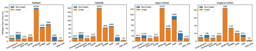
Figure 7: Runtime Details. The orange bar corresponds to training time per minibatch spending on GNNs. The blue bar corresponds to training time per minibatch except for GNNs. The values ahead of each bar correspond to time cost of each color. The first one corresponds to blue bar (non-graph), and the other one corresponds to the orange bar (graph). We can see that GNNs occupy the majority of training time cost.

Table 8: CPU runtime on Brain10. We show the CPU runtime on graph and non-graph operations on Brain10. We also provide number of edges used in graph convolutions in “Conv. Edges” column. We can see that on Brain10, we have a large amount of edges, and aggregation of our proposal does not significantly reduce the number of edges. Thus the GNN computation cost even increases since the edge attributes are more complex than time-and-graph baselines. Furthermore, since we have a large amount of edges, the time cost for RNN on edge attributes of our proposal is also extremely high.

Representation	Model	Graph	Non-Graph	Conv. Edges
graph-then-time	EvolveGCN-O	557 ms	21 ms	1955488
graph-then-time	EvolveGCN-H	533 ms	57 ms	1955488
graph-then-time	GCN-GRU	51 ms	26 ms	1955488
graph-then-time	DySAT	150 ms	43 ms	1955488
time-and-graph	GCRN-M2	5940 ms	7 ms	1955488
time-and-graph	DCRNN	3542 ms	17 ms	1955488
time-then-graph	TGAT	7282 ms	89 ms	1955488
time-then-graph	TGN	2376 ms	409 ms	1955488
time-then-graph	GRU-GCN	975 ms	14638 ms	1761414

We show the training runtime proportions of GNNs and non-GNNs for each model in Figure 7.

We can see the GCRN-M2 and DCRNN as the slowest two methods, spend nearly all of their time on GNNs. This is because they have multiple GNNs as Equation 5 while all the other methods only have a single GNN. For example, for GCRN-M2 whose sequence representation is LSTM, it will have 8 different GNNs: It has two GNNs for input gate, forget gate, output gate and cell unit respectively.

In the constrast, graph-then-time models (EvolveGCNs, GCN-GRU and DySAT) as a subset of time-and-graph, is faster. This is because they only have GNN on input snapshots, and do not have GNN depending on hidden representation from previous snapshots (see Equation 6). Thus, graph-then-time can compute GNN for different snapshots in the same time. Besides, it does not require multiple GNNs as in time-and-graph models. These two advantages result in a great improvement on efficiency comparing with time-and-graph baselines (GCRN-M2, DCRNN).

Our proposal GRU-GCN spends very small amount of runtime on GNNs. This is because GRU-GCN is applied on the aggregated temporal graph which has far less amount of edges comparing to snapshotted temporal graphs in those datasets. In the meanwhile, our proposal GRU-GCN also spends small amount of runtime on non-graph operations, e.g., RNNs, which eventually results in its great efficiency. Pay attention that RNN on edge attributes has small cost only because we are using simple GRU representation and the number of edges are small on studying datasets. However, this is not true when we have large amount of edges. e.g., when the temporal graph is dense.

Indeed, Table 8 finds that GRU-GCN is slowest on Brain10 where the number of edges is very large and aggregation does not effectively reduce the number of edges (edges are almost the same as snapshotted form). Although Table 8 is runtimes on CPU rather than GPU, it still reveals that the efficiency of time-then-graph is dependent on temporal graph topologies, and it is not always true that time-then-graph will be more efficient than time-and-graph.

References

- Azizian & Lelarge (2020) Azizian, W. and Lelarge, M. Characterizing the expressive power of invariant and equivariant graph neural networks. arXiv preprint arXiv:2006.15646, 2020.
- Bahdanau et al. (2014) Bahdanau, D., Cho, K., and Bengio, Y. Neural machine translation by jointly learning to align and translate. arXiv preprint arXiv:1409.0473, 2014.
- Battaglia et al. (2016) Battaglia, P., Pascanu, R., Lai, M., Rezende, D. J., and kavukcuoglu, K. Interaction networks for learning about objects, relations and physics. In NIPS’16 Proceedings of the 30th International Conference on Neural Information Processing Systems, volume 29, pp. 4509–4517, 2016.
- Berger-Wolf & Saia (2006) Berger-Wolf, T. Y. and Saia, J. A framework for analysis of dynamic social networks. In Proceedings of the 12th ACM SIGKDD international conference on Knowledge discovery and data mining, pp. 523–528, 2006.
- Bodnar et al. (2021) Bodnar, C., Frasca, F., Otter, N., Wang, Y., Lio, P., Montufar, G. F., and Bronstein, M. Weisfeiler and lehman go cellular: Cw networks. Advances in Neural Information Processing Systems, 34:2625–2640, 2021.
- Chen et al. (2018) Chen, J., Xu, X., Wu, Y., and Zheng, H. Gc-lstm: Graph convolution embedded lstm for dynamic link prediction. arXiv preprint arXiv:1812.04206, 2018.
- Chen et al. (2019a) Chen, J., Zhang, J., Xu, X., Fu, C., Zhang, D., Zhang, Q., and Xuan, Q. E-lstm-d: A deep learning framework for dynamic network link prediction. IEEE Transactions on Systems, Man, and Cybernetics, pp. 1–14, 2019a.
- Chen et al. (2019b) Chen, Z., Li, L., and Bruna, J. Supervised community detection with line graph neural networks. In 7th International Conference on Learning Representations, ICLR 2019, 2019b.
- Chen et al. (2019) Chen, Z., Villar, S., Chen, L., and Bruna, J. On the equivalence between graph isomorphism testing and function approximation with gnns. Advances in neural information processing systems, 32, 2019.
- Cho et al. (2014) Cho, K., van Merrienboer, B., Gulcehre, C., Bahdanau, D., Bougares, F., Schwenk, H., and Bengio, Y. Learning phrase representations using rnn encoder–decoder for statistical machine translation. In Proceedings of the 2014 Conference on Empirical Methods in Natural Language Processing (EMNLP), pp. 1724–1734, 2014.
- Chung et al. (2014) Chung, J., Çaglar Gülçehre, Cho, K., and Bengio, Y. Empirical evaluation of gated recurrent neural networks on sequence modeling. arXiv preprint arXiv:1412.3555, 2014.
- Cotta et al. (2021) Cotta, L., Morris, C., and Ribeiro, B. Reconstruction for powerful graph representations. Advances in Neural Information Processing Systems, 34, 2021.
- Cui et al. (2020) Cui, Z., Henrickson, K., Ke, R., and Wang, Y. Traffic graph convolutional recurrent neural network: A deep learning framework for network-scale traffic learning and forecasting. IEEE Transactions on Intelligent Transportation Systems, 21:4883–4894, 2020.
- da Xu et al. (2020) da Xu, chuanwei ruan, evren korpeoglu, sushant kumar, and kannan achan. Inductive representation learning on temporal graphs. In ICLR 2020 : Eighth International Conference on Learning Representations, 2020.
- Defferrard et al. (2016) Defferrard, M., Bresson, X., and Vandergheynst, P. Convolutional neural networks on graphs with fast localized spectral filtering. In NIPS’16 Proceedings of the 30th International Conference on Neural Information Processing Systems, volume 29, pp. 3844–3852, 2016.
- Dehmamy et al. (2019) Dehmamy, N., Barabasi, A.-L., and Yu, R. Understanding the representation power of graph neural networks in learning graph topology. In Advances in Neural Information Processing Systems, volume 32, pp. 15413–15423, 2019.
- Deng et al. (2019) Deng, S., Wang, S., Rangwala, H., Wang, L., and Ning, Y. Graph message passing with cross-location attentions for long-term ili prediction. arXiv preprint arXiv:1912.10202, 2019.
- Douglas (2011) Douglas, B. L. The weisfeiler-lehman method and graph isomorphism testing. arXiv preprint arXiv:1101.5211, 2011.
- Duvenaud et al. (2015) Duvenaud, D., Maclaurin, D., Aguilera-Iparraguirre, J., Gómez-Bombarelli, R., Hirzel, T., Aspuru-Guzik, A., and Adams, R. P. Convolutional networks on graphs for learning molecular fingerprints. In NIPS’15 Proceedings of the 28th International Conference on Neural Information Processing Systems - Volume 2, volume 28, pp. 2224–2232, 2015.
- Dwivedi et al. (2020) Dwivedi, V. P., Joshi, C. K., Laurent, T., Bengio, Y., and Bresson, X. Benchmarking graph neural networks. arXiv preprint arXiv:2003.00982, 2020.
- Fallani et al. (2014) Fallani, F. D. V., Richiardi, J., Chavez, M., and Achard, S. Graph analysis of functional brain networks: practical issues in translational neuroscience. Philosophical Transactions of the Royal Society B, 369:20130521–20130521, 2014.
- Fout et al. (2017) Fout, A., Byrd, J., Shariat, B., and Ben-Hur, A. Protein interface prediction using graph convolutional networks. In Advances in Neural Information Processing Systems, volume 30, pp. 6530–6539, 2017.
- Gao et al. (2021) Gao, J., Sharma, R., Qian, C., Glass, L. M., Spaeder, J., Romberg, J., Sun, J., and Xiao, C. Stan: spatio-temporal attention network for pandemic prediction using real-world evidence. Journal of the American Medical Informatics Association, 28(4):733–743, 2021.
- Gilmer et al. (2017) Gilmer, J., Schoenholz, S. S., Riley, P. F., Vinyals, O., and Dahl, G. E. Neural message passing for quantum chemistry. In Proceedings of the 34th International Conference on Machine Learning - Volume 70, pp. 1263–1272, 2017.
- Gori et al. (2005) Gori, M., Monfardini, G., and Scarselli, F. A new model for learning in graph domains. In Proceedings. 2005 IEEE International Joint Conference on Neural Networks, 2005., volume 2, pp. 729–734, 2005.
- Goyal et al. (2018) Goyal, P., Kamra, N., He, X., and Liu, Y. Dyngem: Deep embedding method for dynamic graphs. arXiv preprint arXiv:1805.11273, 2018.
- Goyal et al. (2020) Goyal, P., Chhetri, S. R., and Canedo, A. dyngraph2vec: Capturing network dynamics using dynamic graph representation learning. Knowledge Based Systems, 187:104816, 2020.
- Guo et al. (2019) Guo, S., Lin, Y., Feng, N., Song, C., and Wan, H. Attention based spatial-temporal graph convolutional networks for traffic flow forecasting. In Proceedings of the AAAI Conference on Artificial Intelligence, volume 33, pp. 922–929, 2019.
- Hajiramezanali et al. (2019) Hajiramezanali, E., Hasanzadeh, A., Narayanan, K. R., Duffield, N., Zhou, M., and Qian, X. Variational graph recurrent neural networks. In Advances in neural information processing systems, volume 32, pp. 10701–10711, 2019.
- Hand & Till (2001) Hand, D. J. and Till, R. J. A simple generalisation of the area under the roc curve for multiple class classification problems. Machine learning, 45(2):171–186, 2001.
- Hochreiter & Schmidhuber (1997) Hochreiter, S. and Schmidhuber, J. Long short-term memory. Neural Computation, 9(8):1735–1780, 1997.
- Huang et al. (2021) Huang, H., Shi, R., Zhou, W., Wang, X., Jin, H., and Fu, X. Temporal heterogeneous information network embedding. In IJCAI, pp. 1470–1476, 2021.
- Jin et al. (2020) Jin, G., Wang, Q., Zhu, C., Feng, Y., Huang, J., and Zhou, J. Addressing crime situation forecasting task with temporal graph convolutional neural network approach. In 2020 12th International Conference on Measuring Technology and Mechatronics Automation (ICMTMA), 2020.
- Kapoor et al. (2020) Kapoor, A., Ben, X., Liu, L., Perozzi, B., Barnes, M., Blais, M., and O’Banion, S. Examining covid-19 forecasting using spatio-temporal graph neural networks. arXiv preprint arXiv:2007.03113, 2020.
- Keriven & Peyré (2019) Keriven, N. and Peyré, G. Universal invariant and equivariant graph neural networks. In Advances in Neural Information Processing Systems (NeurIPS), volume 32, pp. 7092–7101, 2019.
- Kileel et al. (2019) Kileel, J., Trager, M., and Bruna, J. On the expressive power of deep polynomial neural networks. In 33rd Annual Conference on Neural Information Processing Systems, NeurIPS 2019, volume 32, pp. 10310–10319, 2019.
- Kipf & Welling (2016) Kipf, T. N. and Welling, M. Semi-supervised classification with graph convolutional networks. In ICLR (Poster), 2016.
- Lei et al. (2019) Lei, K., Qin, M., Bai, B., Zhang, G., and Yang, M. Gcn-gan: A non-linear temporal link prediction model for weighted dynamic networks. In IEEE INFOCOM 2019 - IEEE Conference on Computer Communications, pp. 388–396, 2019.
- Leman & Weisfeiler (1968) Leman, A. and Weisfeiler, B. A reduction of a graph to a canonical form and an algebra arising during this reduction. Nauchno-Technicheskaya Informatsiya, 2(9):12–16, 1968.
- Li et al. (2019) Li, J., Han, Z., Cheng, H., Su, J., Wang, P., Zhang, J., and Pan, L. Predicting path failure in time-evolving graphs. In Proceedings of the 25th ACM SIGKDD International Conference on Knowledge Discovery & Data Mining, pp. 1279–1289, 2019.
- Li et al. (2016) Li, Y., Tarlow, D., Brockschmidt, M., and Zemel, R. S. Gated graph sequence neural networks. In ICLR (Poster), 2016.
- Li et al. (2018) Li, Y., Yu, R., Shahabi, C., and Liu, Y. Diffusion convolutional recurrent neural network: Data-driven traffic forecasting. In International Conference on Learning Representations, 2018.
- Loukas (2020) Loukas, A. What graph neural networks cannot learn: depth vs width. In ICLR 2020 : Eighth International Conference on Learning Representations, 2020.
- Lv et al. (2020) Lv, M., Hong, Z., Chen, L., Chen, T., Zhu, T., and Ji, S. Temporal multi-graph convolutional network for traffic flow prediction. IEEE Transactions on Intelligent Transportation Systems, pp. 1–12, 2020.
- Makarov et al. (2021) Makarov, I., Savchenko, A., Korovko, A., Sherstyuk, L., Severin, N., Mikheev, A., and Babaev, D. Temporal graph network embedding with causal anonymous walks representations. arXiv preprint arXiv:2108.08754, 2021.
- Manessi et al. (2020) Manessi, F., Rozza, A., and Manzo, M. Dynamic graph convolutional networks. Pattern Recognition, 97:107000, 2020.
- Maron et al. (2019a) Maron, H., Ben-Hamu, H., Serviansky, H., and Lipman, Y. Provably powerful graph networks. In Advances in Neural Information Processing Systems, volume 32, pp. 2153–2164, 2019a.
- Maron et al. (2019b) Maron, H., Fetaya, E., Segol, N., and Lipman, Y. On the universality of invariant networks. In International Conference on Machine Learning, pp. 4363–4371, 2019b.
- Morris et al. (2019) Morris, C., Ritzert, M., Fey, M., Hamilton, W. L., Lenssen, J. E., Rattan, G., and Grohe, M. Weisfeiler and leman go neural: Higher-order graph neural networks. In Proceedings of the AAAI Conference on Artificial Intelligence, volume 33, pp. 4602–4609, 2019.
- Murphy et al. (2019) Murphy, R. L., Srinivasan, B., Rao, V. A., and Ribeiro, B. Relational pooling for graph representations. In International Conference on Machine Learning, pp. 4663–4673, 2019.
- Nguyen & Maehara (2020) Nguyen, H. and Maehara, T. Graph homomorphism convolution. In International Conference on Machine Learning, pp. 7306–7316. PMLR, 2020.
- Panagopoulos et al. (2020) Panagopoulos, G., Nikolentzos, G., and Vazirgiannis, M. Transfer graph neural networks for pandemic forecasting. arXiv, 2020.
- Pareja et al. (2020) Pareja, A., Domeniconi, G., Chen, J., Ma, T., Suzumura, T., Kanezashi, H., Kaler, T., Schardl, T. B., and Leiserson, C. E. Evolvegcn: Evolving graph convolutional networks for dynamic graphs. In Proceedings of the AAAI Conference on Artificial Intelligence, volume 34, pp. 5363–5370, 2020.
- Rahman et al. (2018) Rahman, M., Saha, T. K., Hasan, M. A., Xu, K. S., and Reddy, C. K. Dylink2vec: Effective feature representation for link prediction in dynamic networks. arXiv preprint arXiv:1804.05755, 2018.
- Rossi et al. (2020) Rossi, E., Chamberlain, B., Frasca, F., Eynard, D., Monti, F., and Bronstein, M. M. Temporal graph networks for deep learning on dynamic graphs. arXiv preprint arXiv:2006.10637, 2020.
- Sankar et al. (2020) Sankar, A., Wu, Y., Gou, L., Zhang, W., and Yang, H. Dysat: Deep neural representation learning on dynamic graphs via self-attention networks. In Proceedings of the 13th International Conference on Web Search and Data Mining, pp. 519–527, 2020.
- Scarselli et al. (2005) Scarselli, F., Yong, S. L., Gori, M., Hagenbuchner, M., Tsoi, A. C., and Maggini, M. Graph neural networks for ranking web pages. In Proceedings of the 2005 IEEE/WIC/ACM International Conference on Web Intelligence, pp. 666–672, 2005.
- Seo et al. (2018) Seo, Y., Defferrard, M., Vandergheynst, P., and Bresson, X. Structured sequence modeling with graph convolutional recurrent networks. In International Conference on Neural Information Processing, pp. 362–373, 2018.