Low overhead fault-tolerant quantum error correction with the surface-GKP code
Abstract
Fault-tolerant quantum error correction is essential for implementing quantum algorithms of significant practical importance. In this work, we propose a highly effective use of the surface-GKP code, i.e., the surface code consisting of bosonic GKP qubits instead of bare two-level qubits. In our proposal, we use error-corrected two-qubit gates between GKP qubits and introduce a maximum likelihood decoding strategy for correcting shift errors in the two-GKP-qubit gates. Our proposed decoding reduces the total CNOT failure rate of the GKP qubits, e.g., from to at a GKP squeezing of dB, compared to the case where the simple closest-integer decoding is used. Then, by concatenating the GKP code with the surface code, we find that the threshold GKP squeezing is given by dB under the the assumption that finite-squeezing of the GKP states is the dominant noise source. More importantly, we show that a low logical failure rate can be achieved with moderate hardware requirements, e.g., modes and qubits at a GKP squeezing of dB as opposed to bare qubits for the standard rotated surface code at an equivalent noise level (i.e., ). Such a low failure rate of our surface-GKP code is possible through the use of space-time correlated edges in the matching graphs of the surface code decoder. Further, all edge weights in the matching graphs are computed dynamically based on analog information from the GKP error correction using the full history of all syndrome measurement rounds. We also show that a highly-squeezed GKP state of GKP squeezing dB can be experimentally realized by using a dissipative stabilization method, namely, the Big-small-Big method, with fairly conservative experimental parameters. Lastly, we introduce a three-level ancilla scheme to mitigate ancilla decay errors during a GKP state preparation.
I Introduction
Despite various opportunities offered by noisy intermediate-scale quantum (NISQ) devices [1], fault-tolerant quantum error correction techniques [2] are essential for executing quantum algorithms intractable by classical computers such as integer factorization [3] and the simulation of real-time dynamics of large quantum systems [4]. One of the most promising approaches towards fault-tolerant quantum computing is to implement the surface code [5] (or its variants) using bare two-level qubits such as transmons [6, 7] or internal states of trapped ions [8].
Recently, however, it has become increasingly clear that bosonic qubits (error corrected via bosonic quantum error correction [9, 10, 11]) provide unique advantages that are not available to bare two-level qubits. For instance, two-component cat codes (consisting of two coherent states ) [12, 13, 14, 15, 16] naturally realize noise-biased qubits whose bit-flip error rate is exponentially suppressed in the size of the code , whereas the phase-flip error rate increases only linearly in . Most importantly, a CNOT gate between these two noise-biased cat qubits can be performed in a bias-preserving way. That is, high noise bias (towards phase-flip errors) can be maintained during the entire execution of the CNOT gate through a suitably designed control scheme [17, 18, 19, 20]. On the other hand, as shown in Ref. [21], a bias-preserving CNOT gate is not possible with strictly two-dimensional bare qubits. In recent proposals [17, 19, 20], the unique noise-bias feature of bosonic cat qubits has been utilized to significantly reduce the required resource overheads for implementing fault-tolerant quantum computation.
GKP qubits [22, 23, 24, 25, 26] are another example of bosonic qubits which enjoy unique advantages unavailable to bare two-level qubits: if GKP qubits are used to implement a next-level error-correcting code (e.g., the surface code), extra analog information gathered from GKP error correction [27] can inform us which GKP qubits are more likely to have had an error. Thus, by incorporating the extra analog information to the decoder of the next-level code, one can significantly boost the performance of the next-level error-correcting code [27, 28, 29, 30, 31, 32, 33, 34, 35]. While it has been shown that bare two-level qubits can also benefit from analog information in a limited context of qubit readout [36, 37], bare two-level qubits do not have access to analog information in a more general setting such as during gates.
In this paper, we propose a highly optimized version of the surface-GKP code (i.e., concatenation of the GKP code with the surface code), building on remarkable recent progress in the study of GKP codes. In particular, assuming that the finite squeezing of the GKP states is the only noise source (see Section II.3 for a justification), we show that the threshold GKP squeezing of our surface-GKP code is given by dB, which is lower than all reported threshold values of the GKP squeezing in the literature under the same noise model and without the use of post-selection. Our threshold dB is also close to the GKP squeezing of dB which was experimentally achieved in a circuit QED system [25].
While the fault-tolerance threshold is an important metric, it is even more important to study the behavior of logical error rates below the threshold. That is, it is crucial to understand how many hardware elements are needed to achieve a target logical error rate to estimate an overall cost of a fault-tolerance method. For instance, while there are measurement-based schemes that achieve a very low GKP squeezing threshold (e.g., dB) with the help of post-selection [28, 31], it is not yet clear if the overall resource overhead is manageable in practice despite the use of post-selection.
Hence, going beyond the discussion of fault-tolerant thresholds, we further demonstrate that our surface-GKP code can achieve low logical error rates with moderate resource costs at a reasonable value of GKP squeezing. For instance, we show that a logical error rate per code cycle can be achieved with only oscillator modes and qubits at a moderately high GKP squeezing of dB. On the other hand, to achieve a similar logical failure rate , the standard surface code approach is estimated to require at least bare qubits at an equivalent noise level using a toy circuit-level depolarizing noise model (see Figs. 6b and 3). Moreover, we show in Section IV that a highly-squeezed GKP state with GKP squeezing dB can be experimentally realized by using dissipative stabilization methods [38] (and our modification of them to mitigate ancilla qubit errors) assuming fairly conservative experimental parameters. We also consider the use of noise-biased ancilla qubits (in a similar spirit as in Ref. [39]) by using a rectangular-lattice GKP code for the surface code ancilla qubits. We conclude that using such biased qubits provide no improvements when the GKP squeezing is below dB and a very minor improvement when the GKP squeezing is dB (see Fig. 7).
To achieve a low logical error rate with only moderate resource requirements, we adopt the teleportation-based GKP error correction [40] in our surface-GKP code proposal, instead of the more widely used Steane-type GKP error correction [22]. In the literature, discussions on the use of teleportation-based method have been centered around the fact that it does not require online squeezing operations which is particularly convenient for optical systems [40, 32, 33]. In Section II.2, however, we emphasize the performance aspect of the teleportation-based method and thus motivate the use of it even in systems where online squeezing operations are not much harder to implement than beam-splitter interactions. We also adopt the recent idea of performing GKP error correction four times for each surface code stabilizer measurement [33], as opposed to applying them only once per every syndrome extraction [29, 30]. By doing so, every two-qubit gate between GKP qubits is error corrected.
The key contributions of our work are as follows: first, we introduce a maximum likelihood decoding method for decoding shift errors in the error-corrected two-qubit gates (i.e., CNOT and CZ gates) between GKP qubits. We then demonstrate that our maximum likelihood decoding method significantly outperforms the simple, more widely used closest-integer decoding method. For instance, while the closest-integer decoding yields a total CNOT failure rate of at a GKP squeezing of dB, our maximum likelihood decoding achieves a CNOT failure rate of at the same GKP squeezing (the gap gets wider as we increase the GKP squeezing; see Table 1). Secondly, we add space-time correlated edges in the matching graphs of the surface code decoder. In addition, we provide a detailed method for dynamically computing all edge weights after incorporating the extra analog information from all GKP error corrections over the full syndrome measurement history. Adding space-time correlated edges is especially crucial in the case where every two-qubit gate is error corrected because doing so introduces errors that are correlated both in space and time in the surface code error correction. Lastly, we systematically analyze dissipative methods [38] for stabilizing a highly-squeezed GKP state and show that the Big-small-Big method is particularly well suited for preparing a highly-squeezed GKP state. Moreover, we propose to use a three-level ancilla to mitigate ancilla decay errors and demonstrate that a high decay rate in the ancilla can be tolerated. Note that the ancilla here refers to an ancilla for stabilizing a GKP state and should be distinguished from the ancilla GKP qubits in the surface-GKP code.
Our paper is organized as follows. In Section II, we review basic properties of the GKP qubits and compare two GKP error correction methods, namely, Steane-type and teleportation-based GKP error correction methods. Most importantly, in Section II.3, we introduce a maximum likelihood decoding method for error-corrected two qubit gates between GKP qubits and show that it significantly outperforms the closest-integer decoding. In Section III, we present the main results regarding the logical failure rates of our highly optimized surface-GKP code (see Fig. 6b) and compare the resource overheads of our scheme with the standard surface code approach based on bare qubits (see Table 3). In Section IV, we discuss the experimental feasibility of a highly-squeezed GKP state and introduce a three-level ancilla technique for mitigating ancilla decay errors. Lastly, we conclude the paper with discussion and outlook in Section V.
II Rectangular-lattice GKP code
Here, we review the rectangular-lattice GKP code, Steane-type, and teleportation-based GKP error correction schemes. We also propose a maximum likelihood decoding method for correcting shift errors during an error-corrected two-qubit gate between GKP qubits. In particular, for two-GKP qubit gates (e.g., CNOT gate), we consider a hybrid scheme where the control qubit (to be used as an ancilla qubit in the surface code) is encoded in a rectangular-lattice GKP code and the target qubit (to be used as a data qubit) is encoded in the square-lattice GKP code.
We choose to focus on the hybrid scheme instead of the homogeneous scheme where both qubits are encoded in the same rectangular-lattice GKP code. The homogeneous scheme was considered in Ref. [41] to bias the noise of the GKP qubits and was shown to be advantageous in the high noise regime for a code capacity noise model (i.e., without considering finite squeezing of GKP states). In our case, however, we are mainly concerned with the finite GKP squeezing as it is the most dominant noise source in practical scenarios (see Section II.3 for a more quantitative discussion). In this case, in the practically relevant regime of GKP squeezing between dB and dB, we found that the enhanced phase-flip rate in the homogeneous scheme is too large to be compensated by any advantages from a reduced bit-flip rate.
On the other hand, a key motivation behind the hybrid scheme is to bias the noise only in the ancilla qubits of the surface code such that the noise back-propagation from an ancilla qubit to the data block is reduced at the expense of increased syndrome measurement error rate (in the same spirit as in Ref. [39]; see also Table 2). In this case, we do observe a very minor improvement over the case where we use the noise-unbiased square-lattice GKP qubits everywhere. Although we end up focusing on the square-lattice GKP code, we review the more general rectangular-lattice GKP codes to explicitly demonstrate the optimality (or near-optimality) of the square-lattice GKP code.
II.1 Logical states, operations. and measurements
Rectangular-lattice GKP code states are stabilized by two commuting displacement operators
| (1) |
Note that the case corresponds to the square-lattice GKP code and as will be made clear shortly, the parameter determines the aspect ratio of the underlying rectangular lattice. The logical Pauli operators are given by
| (2) |
Thus, the logical states in the computational basis (eigenstates of ) are given by
| (3) |
and the logical states in the complementary basis (eigenstates of ) are given by
| (4) |
Note that the position and momentum quadratures of the logical states sit on a rectangular lattice . Thus, compared to the square-lattice case (i.e., ), the spacing in the position quadrature is elongated by a factor of and the spacing in the momentum quadrature is contracted by the same factor. In terms of the error-correcting capability, this means that the rectangular-lattice GKP code can correct any small shift error with
| (5) |
As a result, choosing and assuming that noise is symmetric in both the position and the momentum quadratures (which is typically the case; see, e.g., Section II.2), the rectangular-lattice GKP code has a higher chance of having a logical error than a logical error. The opposite is true for .
Regardless of the underlying lattice structure of the GKP code, logical Clifford operations of the GKP code can be performed by using a Gaussian operation (or a quadratic Hamiltonian in the quadrature operators). The most relevant Clifford operations to the implementation of the surface code are the CNOT and the CZ gates. In our surface code architecture, we consider a hybrid code where the ancilla qubits of the surface code are encoded in a rectangular-lattice GKP code but the data qubits are always encoded in the square-lattice GKP code. Thus, we assume that the control qubit of the CNOT gate is a rectangular-lattice GKP qubit with and the target qubit is a square-lattice GKP qubit with . Such a CNOT gate can be implemented by using a rescaled SUM gate (or a coupling)
| (6) |
where is the control qubit and is the target qubit. Similarly, the CZ gate between a rectangular-lattice GKP qubit and a square-lattice GKP qubit can be realized via a coupling:
| (7) |
where the qubit is encoded in a rectangular-lattice GKP code and the qubit is encoded in the square-lattice GKP qubit.
Lastly, we remark that the -basis measurement (distinguishing from ) can be performed by a position homodyne measurement. More specifically, if the position homodyne measurement outcome is in the range for an even (odd) , we infer that the state is in (). Similarly, the -basis measurement can be done by a momentum homodyne measurement: if the measurement outcome is in the range for an even (odd) , we infer that the state is in ().
II.2 Teleportation-based GKP error correction
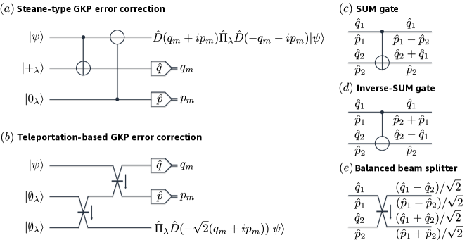
To correct for the shift errors with the GKP code, it is essential to non-destructively measure quadrature operators modulo an appropriate spacing (e.g., modulo and modulo in the case of the rectangular-lattice GKP code). In the original GKP paper [22], it was proposed to achieve this via a Steane-type error correction by using two ancilla GKP states , , the SUM gate and its inverse, and homodyne measurements (see Fig. 1 (a)). Recently, Ref. [40] proposed an alternative method, namely a teleportation-based GKP error correction method, which requires two identical ancilla GKP states (to be defined below), beam-splitter interactions, and homodyne measurements (see Fig. 1 (b)).
One of the advantages of the teleportation-based GKP error correction, as advocated in Refs. [40, 32, 33], is that it works with beam-splitter interactions and does not require any online squeezing operations. On the other hand, the Steane-type GKP error correction is based on the SUM gate and its inverse which do require squeezing operations in addition to beam-splitter interactions. The absence of squeezing operations in the teleportation-based method is especially convenient for optical systems since beam-splitter interactions are much easier to realize than squeezing operations in the optics setting. In superconducting systems, however, engineering the SUM gate is not quite harder than engineering a beam-splitter interaction because one can simply add more drive tones to realize the extra squeezing operations on top of the beam-splitter interaction [42, 43, 44].
In this section, we review both the Steane-type and the teleportation-based GKP error correction schemes. In particular, we pay particular attention to the performance aspect of these two schemes and emphasize that the teleportation-based method performs better than the Steane-type method under the same condition on the quality of the ancilla GKP states. That is, the teleportation-based method is a better choice than the Steane-type method for any systems regardless of whether online squeezing operations are hard to implement or not.
Since the teleportation-based GKP error correction was only recently introduced but is crucial for boosting the performance of the GKP code, we review it as well as the Steane-type GKP error correction in great detail. In Section II.2.1, we first focus on the case where ancilla GKP states are noiseless and present the key ideas behind both GKP error correction schemes. The adverse effects of noisy ancilla GKP states will be discussed in Section II.2.2.
II.2.1 Noiseless ancilla GKP states
In the Steane-type GKP error correction (shown in Fig. 1 (a)), the ancilla which is initially prepared in non-destructively measures the position of the state modulo . Similarly the other ancilla which is initially in measures the momentum of the state modulo in a non-destructive manner. As a result, conditioned on the measurement outcomes and , the output state is given by
| (8) |
where is the projection operator to the GKP code space and is the displacement operator (see Appendix A for the derivation). Note that our convention for the displacement operator, which is suitable for describing the GKP code, is different from the usual convention by a factor of in the shift argument, i.e., . Note also that the non-destructiveness of the measurement is evident once we view as the projection operator to a displaced GKP code space by .
Since the output state is in a displaced GKP code space, such shift needs to be corrected. This is done by applying a correction shift , where the size of the correction shift is given by
| (9) |
Here, the remainder function is defined as
| (10) |
By using the remainder function in the correction shifts, we are employing a maximum likelihood decoding strategy under the assumption that smaller shifts are more likely to happen than larger shifts (this assumption is not necessarily true in the case of the CNOT and the CZ gates; see Section II.3 for more details). Through this decoding strategy, we can correct any small shifts such that and .
In the teleportation-based GKP error correction scheme (shown in Fig. 1 (b)), both ancilla modes are initialized in the GKP qunaught state
| (11) |
Ref. [40] called a “qunaught” state because it is the unique state of the rectangular-lattice GKP code that encodes only one logical state, hence carrying no quantum information (note the additional factor of in the lattice spacing in Eq. 11 compared to the logical states of a GKP qubit in Eqs. 3 and 4). The GKP qunaught state has also been called the grid state [45] or the canonical GKP state [46, 47] in different contexts.
Define the beam-splitter unitary operator between the modes and as
| (12) |
In the Heisenberg picture, the quadrature operators are transformed via the beam-splitter unitary as follows:
| (13) |
Thus, we have a balanced beam-splitter interaction at . Applying the balanced beam-splitter interaction between the two GKP qunaught states and , we get an encoded GKP-Bell state, i.e.,
| (14) |
Once the GKP-Bell state is prepared, we apply the beam-splitter interaction between the modes and which is then followed by homodyne measurements of the quadrature oepratores , . Such a measurement is the continuous-variable analog of the Bell measurement. Thus, the circuit in Fig. 1 (b) implements quantum teleportation from the mode to mode . This is why it is called a teleportation-based GKP error correction scheme. As a result, conditioned on the measurement outcomes and , the output state is given by (see Appendix A for the derivation)
| (15) |
In contrast to the Steane error correction case, the output state of the teleportation-based GKP error correction always is in the GKP code space, not a displaced one, regardless of the measurement outcomes (assuming noiseless ancilla GKP states). However, just like in the case of the discrete-variable qubit teleporation, even if the input state is an ideal GKP encoded state, the teleported state may differ from the input state by a logical Pauli operator depending on the measurement outcome and . More specifically, if the input state is an ideal GKP state, and can only be an integer multiple of and , respectively, i.e., and . Then, the teleported state may differ from the input state by a logical Pauli operator . Such an extra Pauli operator may be physically corrected by applying a suitable correction shift to the teleported state or be kept track of in software via a Pauli frame [48, 49, 50, 51] (until we have to apply a non-Clifford gate).
If the input state is not an ideal GKP state and is instead shifted from the GKP code space, the measurement outcomes multiplied by (i.e., and ) will no longer be an integer multiple of and . In this case, we find the closest integers to and to determine the extra Pauli operator. That is, we set and as
| (16) |
and either physically apply a Pauli correction through a correction shift or keep track of it via a Pauli frame. Similarly as in the case of the Steane-type GKP error correction, by searching for the closest integer, we are employing a maximum likelihood decoding strategy under the same assumption that smaller shifts are more likely than larger shifts (which, again, needs to be revisited in the case of the two-qubit gates between two GKP qubits). Through this decoding strategy, we can correct any small shifts such that and , similarly as in the case of the Steane-type GKP error correction.
II.2.2 Noisy ancilla GKP states
We now discuss the adverse effects of the noise in ancilla GKP states. Since realistic GKP states are only finitely squeezed, they introduce shift errors when they are injected to a GKP error correction circuit. More specifically, a finitely-squeezed GKP state can be understood as a state resulting from applying a coherent Gaussian random shift error (with a noise variance in both the position and the momentum quadratures) to an ideal GKP state. For the purpose of efficient classical simulation of the shift errors, such coherent shift errors are often approximated as incoherent shift errors (i.e., twirling approximation; see, e.g., Appendix A of Ref. [30]).
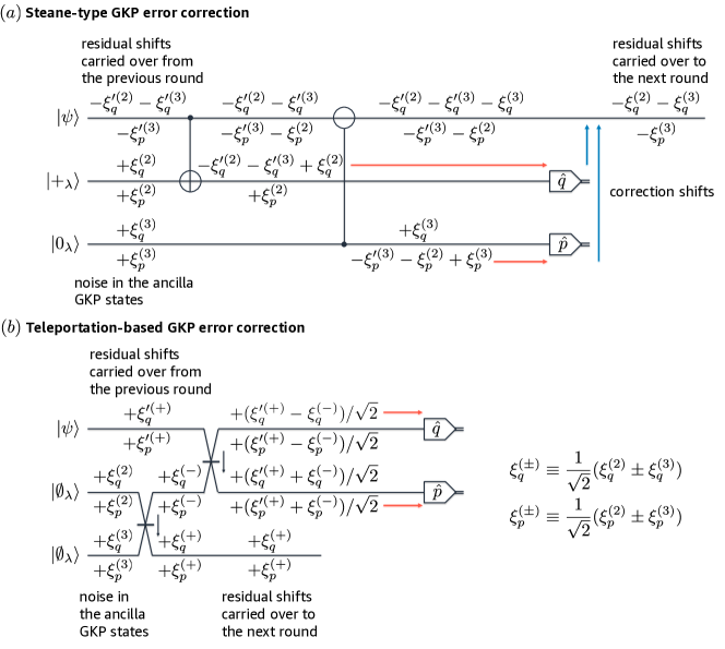
Here, we also make the twirling approximation and assume that the shifts due to finite squeezing are incoherent. More specifically, we assume that each finitely-squeezed GKP state introduces a random shift error where and are randomly drawn from an independent and identically distributed Gaussian distribution with zero mean and noise variance . That is, in both GKP error correction schemes, we assume that the ancilla modes (supporting a GKP state) are corrupted by shift errors (see Fig. 2). Following the same convention in the literature, we define the GKP squeezing (in the unit of decibel) as
| (17) |
where is the variance of the quadrature noise of a vacuum state .
In the case of the Steane-type GKP error correction (shown in Fig. 2 (a)), the data mode inherits residual shifts and from the previous round of the GKP error correction, which will become clear shortly. The position shift is then tranferred to the second ancilla mode via the SUM gate and is added to the ancilla position shift . Thus, the net position shift in the second mode is given by and the measurement outcome of the second mode is given by modulo . In the meantime, an extra position shift is added to the data mode due to transfer of the position shift in the third mode via the inverse-SUM gate. As a result, after applying a correction shift for the position quadrature , the data mode has a residual position shift (modulo )
| (18) |
which is carried over to the next round of the GKP error correction (hence the initial shift in the current round).
In the momentum quadrature, the initial shift is added by an extra shift error transferred from the second mode via the SUM gate. Then, this shift is tranferred to the third mode and is added to the momentum shift in the third mode. Hence, the third mode is corrupted by a net momentum shift and the measurement outcome is given by modulo . After applying a correction momentum shift to the date mode, the data mode has a residual momentum shift (modulo )
| (19) |
which is carried over to the next round (hence initially in the current round).
Note that both the net position shift in the second mode and the net momentum shift in the third mode have a noise variance . If these net shifts are smaller than the correctable shift and , the correction shifts do not cause any logical Pauli errors. However, if they are not, and are given by
| (20) |
with some . Thus, the data GKP qubit is corrupted by a logical Pauli error . The probability of having such a Pauli error is closely related to the weight of the tail of the Gaussian distribution . Note that the factor of in the noise variance is also directly related to the fact that the Glancy-Knill threshold is given by for the square-lattice GKP code [52]. In what follows, we show that the relevant noise variance is given by (instead of ) in the case of the teleportation-based GKP error correction, hence it performs better than the Steane-type method under the same GKP squeezing .
In the case of the teleportation-based GKP error correction (shown in Fig. 2 (b)), the ancilla shift errors are mixed via the balanced beam-splitter interaction. Thus, the third mode (where the state is teleported to) has residual shift errors
| (21) |
which is then carried over to the next round of the GKP error correction. This also means that, in the current round, the data mode inherits residual shifts and from the previous round ( and are defined similarly as and ). After the balanced beam-splitter interaction between the two ancilla modes, the second mode has shift errors
| (22) |
Note that since the quadrature transformation matrix of a beam-splitter interaction is an orthogonal matrix (see Eq. 13), the four shifts are mutually independent just like the untranformed ancilla shifts . The shifts in the second mode are then mixed with the shifts in the data mode and result in a net shift error in the position quadrature and in the momentum quadrature. Thus, the measurement outcomes are given by
| (23) |
As can be seen from Eq. 15, the actual shifts on the data GKP qubit are given by and with an extra factor. Thus, the relevant shifts (to be compared with the lattice spacings and ) are and , whose noise variances are given by . Since the relevant noise variance is smaller in the teleportation-based GKP error correction scheme by a factor of , logical Pauli errors are less likely to occur in the teleportation-based method than in the Steane-type method, given the same GKP squeezing .
Note that since the weight of the Gaussian tail decreases exponentially in the inverse noise variance, the constant factor improvement in the noise variance can bring about a significant decrease in the logical Pauli error probabilities. Apart from the absence of the online squeezing operations and the enhanced resilience against the ancilla GKP noise, we also remark that the teleportation-based scheme is more advantageous for keeping the energy of the encoded state bounded than the Steane-type method. This is thanks to the symmetry between the position and the momentum quadratures in the teleportation-based scheme (which is related to the absence of online squeezing operations). Such a symmetry prevents the Gaussian envelope of the finitely-squeezed GKP states from being distorted during the GKP error correction, and hence always minimizes the energy of the encoded GKP states (see Section A.3 for more details).
II.3 Maximum likelihood decoding for the CNOT and CZ gates between two GKP qubits
Here we consider error-corrected logical two-qubit gates between GKP qubits. That is, we apply GKP error correction right after each logical two-qubit gate. Thus, when analyzing the performance of an error-corrected gate, we assume that each gate is preceded by a GKP error correction from the previous time step and is followed by another GKP error correction which corrects for the shifts accumulated by the end of the gate. In particular, we propose a maximum likelihood decoding for the logical CNOT and CZ gate for the GKP qubits and show that it significantly outperforms the simple closest-integer decoding scheme used, e.g., in Ref. [33].
In the rest of the paper (except for the appendices), we exclusively consider the teleportation-based GKP error correction scheme due to its superior performance over the Steane-based method under the same GKP squeezing. More specifically, we will assume that each GKP error correction is noisy because the ancilla GKP states are only finitely squeezed with a noise variance . Note that in practice, there may be extra noise sources other than the finite GKP squeezing, with photon loss being the most notable example. However, we neglect such extra noise sources in part for simplicity but also because these other noise sources are not appreciable compared to the noise due to the finite GKP squeezing in realistic scenarios.
For instance, the highest GKP squeezing that has been experimentally achieved so far is slightly below . Converting this to the noise variance , we find
| (24) |
at . As explained in the previous section, this noise variance is doubled because there is one carried over from the previous round of the GKP error correction and another one that is added from the current round. Thus, the relevant noise variance due to the finite GKP squeezing is given by at . On the other hand, as shown in Ref. [30], the additional noise variance due to the photon loss is given by (assuming amplification with the same rate), where is the photon loss rate and is the gate time. Thus, if the gate time is times shorter than the single photon relaxation time , the extra noise variance due to the photon loss is only about . Note that even at , we have and thus the noise variance due to finite GKP squeezing dominates. Hence, as a zeroth order approximation, we focus on the case where the finite squeezing of the ancilla GKP states is the only noise source. However, the maximum likelihood decoding method we present here applies to more general cases, e.g., with extra noise due to photon losses.
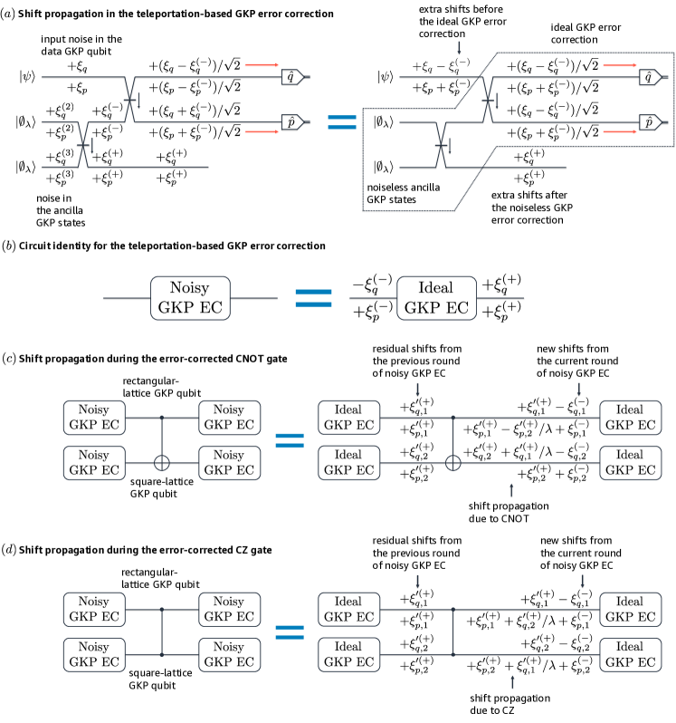
Before analyzing the error-corrected logical CNOT and CZ gate for the GKP qubits, we remark that a noisy (teleportation-based) GKP error correction with finitely-squeezed ancilla GKP states can be understood as an ideal GKP error correction preceded and followeded by extra shift errors and , respectively, where (see Fig. 3 (a) and (b)). This circuit identity will be used throughout the analysis of the error-corrected two qubit gates between GKP qubits.
II.3.1 Error-corrected CNOT gate
Recall that the logical CNOT gate between two GKP qubits can be realized by a coupling (see Eq. 6). Here, we assume that the first qubit is a rectangular-lattice GKP qubit with and the second qubit is the suquare-lattice GKP qubit. As shown in Fig. 3 (c), before the CNOT gate is applied, the GKP qubits inherit shift errors and from the previous round of the noisy GKP error correction. These shifts are propagated through the CNOT gate as and . Then, due to the additional noise from the GKP error correction after the CNOT gate, extra shift errors and are added to the quadratures. Consequently, the two GKP qubits have net shifts
| (25) |
Since all eight underlying shifts and are randomly drawn from an independent and identically distributed Gaussian distribution , we have noise variances and . That is, the position quadrature of the target mode and the momentum quadrature of the control mode have higher noise variances than the other quadratures due to the noise propagation. A motivation for using a rectangular-lattice GKP qubit with in the first qubit is to mitigate the enhanced noise variance via the suppression. However, since the momentum spacing of the first qubit is decreased by a factor of , the error rate on the first qubit is enhanced as a result.
Given these shift errors, the measurement outcomes in the GKP error correction (at the end of the CNOT gate) are given by
| (26) |
Given these measurement outcomes, the goal of the decoding is to correctly infer the four integers . A simple and widely used decoding strategy is to find the closest integers to , , , , i.e.,
| (27) |
For instance, Ref. [33] used the closest-integer decoding to correct for the shift errors in several logical two-qubit gates between GKP qubits (which are equivalent to the CNOT gate up to single-qubit Clifford gates). This way, any net shifts such that , , and can be corrected. Note that the rationale behind the closest-integer decoding is that smaller shifts are more likely to happen than larger shifts. However, we will show below that this is not necessarily the case for the logical two-qubit gates.
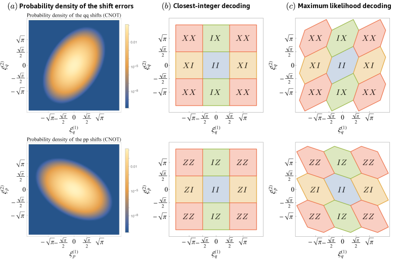
Here, we propose a different decoding strategy, a maximum likelihood decoding, which outperforms the simple closet-integer decoding. Our maximum likelihood decoding is based on an observation that the net shifts errors are mutually correlated. For instance, the net position shifts and are correlated via the propagated shift . More specifically, the position shift vector follows a two-variable Gaussian distribution with zero mean and a covariance matrix
| (28) |
Due to the correlation, shifts in a certain direction are more likely to happen than others. In other words, a larger shift in a preferred direction can occur more often than a smaller shift in a less preferred direction (see the top panel of Fig. 4 (a)). Such a possibility is not taken into account in the simple closest-integer decoding.
Note that the probability density function of the position shifts is given by
| (29) |
where is the determinant of . Then, the goal of our maximum likelihood decoding is as follows. Given the measurement outcomes and , we want to find and such that is maximized, where and . Since is maximized when is minimized, this is equivalent to solving the following optimization problem:
| (30) |
given and . Our algorithm for solving this optimization problem is given in Algorithm 1 in Appendix B.
The decision boundaries of the simple closest-integer decoding and our maximum likelihood decoding are shown in Fig. 4 (b) and (c), respectively. Note that the decision boundaries in the maximum likelihood method are better aligned with the the corresponding probability density functions than the ones in the closest-integer decoding. Thus, there are shifts that can be correctly countered by the maximum likelihood method but are incorrectly mapped to a different lattice point, hence causing a logical Pauli error, in the closest-integer decoding.
Similarly as in the case of the position shifts, the momentum shifts and are also mutually correlated via the propagated shift . Hence, the momentum shift vector follows a two-variable Gaussian distribution with zero mean and a covariance matrix
| (31) |
The probability density function of the momentum shifts and is thus given by (see the bottom panel of Fig. 4 (a))
| (32) |
The goal is the decoding is then to find two integers and , given measurement outcomes and , such that is maximized where and . This can be done by solving the following optimization problem
| (33) |
given and , and our algorithm for solving this optimization problem is given in Algorithm 2 in Appendix B.
II.3.2 Error-corrected CZ gate
The logical CZ gate between a rectangular-lattice GKP qubit and a square-lattice GKP qubit can be realized by a coupling (see Eq. 7). We assume that the first qubit is encoded in a rectangular-GKP code with and the second qubit is encoded in the square-lattice GKP code. Similarly as in the case of the CNOT gate, the GKP qubits inherit shift errors and from the previous round of the noisy GKP error correction before the CZ gate is applied. These shifts are propagated via the CZ gate as and . Then, due to the additional noise from the GKP error correction after the CZ gate, extra shift errors and are added to the quadratures. Consequently, the two GKP qubits have net shifts
| (34) |
See Fig. 3 (d). Then, since the noise correlation structure is equivalent to that of the CNOT gate (up to permutation and sign change), the rest of the analysis, including the maximum likelihood decoding, can be performed in an analogous way.
II.4 Performance of the maximum-likelihood decoding for error-corrected two-GKP-qubit gates
| CNOT logical failure rate | dB | dB | dB | dB | dB |
| Closest-integer decoding | |||||
| Maximum likelihood decoding |
| CNOT logical failure rate | dB | dB | dB | dB |
| Closest-integer decoding | ||||
| Maximum likelihood decoding |
| CX () | CX () | CX () | |
| CZ () | CZ () | CZ () | |
Since the decision boundaries in our maximum-likelihood decoding is better aligned with the underlying probability distribution of the shift errors, the maximum likelihood would outperform the closest-integer decoding. To explicitly show this, we compare in Table 1 the performance of the closest-integer decoding scheme and the maximum likelihood decoding method for the error-corrected CNOT gate between two square-lattice GKP qubits (i.e., ). For all values of the GKP squeezing (from dB to dB), the maximum likelihood decoding method outperforms the simple closest-integer decoding method. In particular, as the GKP squeezing becomes larger, the advantage offered by our maximum likelihood decoding scheme becomes more significant. For instance, while the failure rate of the logical CNOT gate is reduced only by a factor of by using the maximum likelihood decoding at , the reduction factor becomes at . Note that this constant factor reduction significantly reduces the logical error rate when the GKP code is concatenated with the surface code.
Going beyond the square-lattice GKP qubits, we also show how the different error Pauli error rates are changed if the control GKP qubits are replaced by rectangular-GKP qubits. In Table 2, we provide dominant Pauli error probabilities of the error-corrected CNOT and CZ gates between two GKP qubits of GKP squeezing dB. The first qubit is a control qubit and is encoded in the rectangular-lattice GKP code with . Regardless, the second qubit (i.e., the target qubit) is always encoded in the square-lattice GKP code. For both CNOT and CZ gates, we observe that the error on the control qubit is enhanced as we choose . For instance, is increased from to as we increase to . In the surface code architecture, this results in more frequent syndrome measurement errors. On the other hand, the () error rate on the target qubit in the CNOT (CZ) gate is reduced when we use . In particular, () of the CNOT (CZ) gate is decreased from to as we increase to , thanks to the suppression factor in the noise propagation (see, e.g., Eq. 25). In the surface code architecture, this translates to a reduced noise back-propagation to the data block during a surface code stabilizer measurement. Note that the opposite is true for , i.e., increased noise back-propagation to the surface code data block ( to as we go from to ) and reduced ancilla error, hence reducing the syndrome measurement error rate ( to via to ). It is also important to observe that the total CNOT (or CZ) failure rate, i.e., is minimum at .
III Surface-GKP code
In this section, we briefly review the surface-GKP code and present results for logical failure rates of states encoded in the surface-GKP code. In particular, we show that a very low logical error rate (e.g., ) can be achieved by using the square-lattice GKP qubits with a moderately high GKP squeezing of only dB and the surface code distance . We also investigate if the use of noise-biased GKP qubits (with ) in the surface code ancilla can further reduce the logical error rate. We conclude that, under the noise model considered (i.e. when finite squeezing of the GKP states is the only noise source), it is optimal (or very close to optimal) to use the square-lattice GKP qubits everywhere.
III.1 Example experimental setup and decoding methods
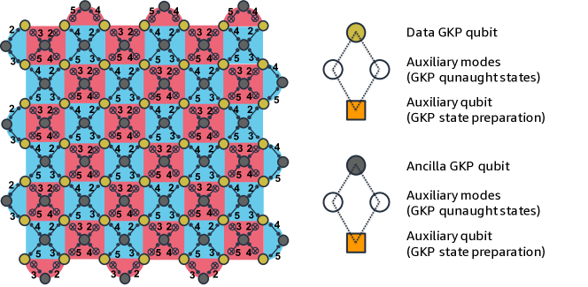
The surface code lattice for a distance surface code (encoding one logical qubit) is illustrated in Fig. 5. Yellow vertices correspond to the data qubits where the logical information is stored, and grey vertices are the ancilla qubits used to measure the surface code stabilizers. The -type stabilizers are represented by red-plaquettes and detect errors whereas -type stabilizers are represented by blue plaquettes and detect errors. The logical operator has minimum support on qubits along each column of the lattice. The logical operator has minimum support on qubits along each row of the lattice. We assume that all the data qubits are encoded in the square-lattice GKP qubit but consider the use of noise-biased rectangular-lattice GKP qubits (i.e., ) for the ancilla qubits. All ancilla qubits in the lattice of Fig. 5 are prepared in the state and measured in the basis via a momentum homodyne measurement. The numbers adjacent to the CNOT and CZ gates indicate the time step at which such gates are applied. We choose the same two-qubit gate scheduling as in Ref. [53].
We apply a (teleportation-based) GKP error correction at the end of each CNOT or CZ gate. That is, each CNOT (or CZ) gate is an error-corrected logical CNOT (or CZ) gate between two GKP qubits as described in Section II.3. Also importantly, since GKP error correction is performed after every two-qubit gate, extra analog information [27, 28, 29, 30, 31, 33, 34] is gathered from the GKP error correction for each two-qubit gate. This analog information can then be used to compute the conditional probabilities of Pauli error rates for each error-corrected CNOT or CZ gate between two GKP qubits. The same applies to the ancilla state preparation, idling, and measurements as well (see Section C.1 for more details). Note that due to the need to implement the GKP error correction to all GKP qubits, each GKP qubit should be assisted by two auxiliary modes (white vertices in Fig. 5) that host two GKP qunaught states and one auxiliary qubit (orange square in Fig. 5) used to prepare the GKP qunaught states. We also emphasize that we use the maximum likelihood decoding instead of the simple closest-integer decoding to correct for shift errors in error-corrected CNOT and CZ gates between two GKP qubits.
In order to ensure a fault-tolerant error correction protocol, measurements of the stabilizers must be repeated at least times [5, 54]. Errors are then corrected using a Minimum Weight Perfect Matching (MWPM) decoder [55] applied to three-dimensional matching graphs with weighted edges which incorporates the conditional probabilities of the GKP error correction for the entire syndrome history. In Section C.2, we provide the matching graphs for and -type stabilizers and show how edge weights can be computed dynamically using analog information from the GKP error correction. It is important to note here that when using the analog information for computing edge weights in the matching graphs, at every time step and in each syndrome measurement round, every fault location (which includes two-qubit gates, idle, state-preparation and ancilla measurements) can have different conditional probabilities associated with a particular Pauli error at the given location. As such, edge weights cannot be pre-computed and must be updated dynamically. Our methods for efficient dynamical updates in the edge weights are described in Section C.2.
III.2 Performance of the surface-GKP code
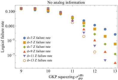
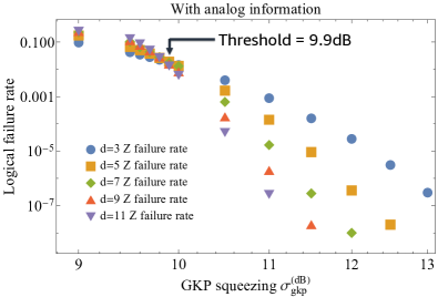
Having described all the methods, we now present the main results, i.e., performance of the surface-GKP code under our highly optimized error correction and decoding procedures. In Fig. 6a, we plot the logical failure rates of the surface-GKP code when analog information from the GKP error correction is omitted. The results are obtained for square surface code patches (i.e. ) with by performing Monte Carlo simulations using the full circuit level noise model described in Appendix C and setting . In Fig. 6b, we plot the logical failure rates of the surface-GKP code when analog information from the GKP error correction is taken into account, and edge weights are dynamically updated following the techniques presented in Section C.2. Note that for the analog simulations, since the logical failure rates drop very quickly with increasing GKP squeezing, we limit the code distance to to avoid large statistical errors from the Monte-Carlo simulations. We omitted plots for the logical error rates since for both cases with and without the use of analog information, logical error rates are nearly identical to the logical error rates shown.
Comparing the plots of Figs. 6a and 6b, it can be seen that using the analog information in the GKP decoding scheme results in smaller logical failure rates by several orders of magnitude. For instance, for and , without the analog information the logical failure rate is found to be compared to when using the analog information, an improvement by a factor of . Such a large improvement is possible since all edge weights of the matching graphs used by the MWPM decoder are determined based on the conditional probabilities of all types of errors in the full history of syndrome measurement rounds given the extra analog information. If GKP qubits are sufficiently squeezed (i.e., ), a Pauli error on GKP qubits occurs due to a shift that is barely larger than the largest correctable shift (e.g., in the case of an idling square-lattice GKP qubit). Hence, most Pauli errors on GKP qubits occur near the decision boundary of a GKP error correction and hence come with a high conditional probability because decisions made near the decision boundary are less reliable than the ones made deep inside the decision boundary (see, e.g., Ref. [30] for a more detailed and quantitative explanation).
For instance, in the case of the distance-three surface code, there are many cases where two faults happened during the three syndrome measurement rounds. These two faults come with high conditional probabilities as they are caused by shifts close the the decision boundary. If this extra analog information (i.e., high conditional probabilities) are not taken into account, the MWPM decoder will choose a wrong path consistent with the syndrome history when pairing highlighted vertices. The correction will then result in a logical Pauli error in the surface-GKP code. However, since the two faults that did happen are likely to have high conditional probabilities, the paths correcting the resulting errors are favored by the MWPM decoder when the analog information is incorporated in the decoding protocol. Thus, even though the distance of the surface code is only three (and hence can only correct at most one fault in the standard surface code setting with bare two-level qubits), many two-fault events are correctable in the surface-GKP code setting with the help of the extra analog information.
We point out that the opposite can also be true in principle. That is, there may be cases where only a single fault occurred but two other candidate fault locations have much higher conditional probabilities despite the fact that no errors were introduced at these other two locations (i.e., false alarms). In this case, the MWPM decoder favors edges of two data qubits not afflicted by an error (due to the large conditional probabilities). The applied correction would then result in a logical Pauli error for the surface-GKP code even though only one fault actually happened (see Section C.3 for a more detailed discussion). Such possibilities might seem problematic from a fault-tolerance perspective. However, such events occur with very small probability (smaller than the computed logical failure rates) and the benefit of using the extra analog information strongly outweighs the side effects due to false alarms. This can be seen from the significantly reduced logical failure rates in Fig. 6b compared to those in Fig. 6a.

From the intersection of the logical failure rate curves in Fig. 6b, the threshold can be seen to be approximately , which represents the lowest threshold to date (see for instance the results in Ref. [33, 34] where the threshold for the same noise model was found to be ). More importantly, however, it can be observed that for some parameter regimes, the logical failure rate curve in Fig. 6b is about three orders of magnitude lower than the one in Ref. [33] (e.g., improved from to at and ).
Note that there are two reasons for the large reduction in the logical failure rate compared to the results of Ref. [33]. First, we use the maximum likelihood decoding for error-corrected CNOT and CZ gates between two GKP qubits. Hence, the total failure rates of the two-qubit gates are significantly reduced at the GKP qubit level (e.g., from to for the CNOT gate at ; see Table 1). Furthermore, since the shift errors are corrected at the end of every two-qubit gates, each two-qubit gate may be afflicted by a Pauli error if the shift errors are incorrectly inferred and countered. Hence, while it was not crucial to use space-time correlated edges in the embodiment of the surface-GKP codes as considered in Refs. [29, 30] (since the GKP error correction is only performed once after all four two-qubit gates per each surface code syndrome measurement), not using space-time correlated edges in the matching graphs in our case (as well as in Ref. [33]) would result in much higher logical failure rates. Such improved performance with space-time correlated edges is primarily due to the fact that GKP error correction is performed after each two-qubit gate, sometimes resulting in an error pattern correlated in both space and time at the surface code level. We can thus conclude that the use of maximum likelihood decoding in the GKP error correction and the space-time correlated edges are the main reasons why the logical error rates are much lower in Fig. 6 compared to what was found in Ref. [33].
Recall that one can change the aspect ratio of the ancilla GKP qubit (i.e., ) to bias the noise towards a certain Pauli error. When , the two-qubit gates in the surface code lattice of Fig. 5 introduce errors on the ancilla qubits with higher probability resulting in increased measurement error rates, while simultaneously reducing the probability of errors on the ancilla qubits thus reducing the rate of space-time correlated errors (a subset of which are hook errors [56]). The opposite is true for (see Table 2). In Fig. 7, we compare logical failure rate curves of surface codes for in increments of . As can be seen, always has the worst performance given the impact of increased space-time correlated errors. For , logical failure rates are always minimized at given the same GKP squeezing , in part due to the fact that the total failure rates of the two-qubit gates are minimized when , as shown in Table 2. For , offers slightly lower failure rates than . For instance, at and , the logical error rate is compared to when . Due to the negligible increase in performance, however, we only plot the logical failure rates for (i.e., square-lattice GKP qubits for all data and ancilla qubits) in Fig. 6.
III.3 Resource overhead comparison
| dB | for | at | # surface code | hardware requirements |
| () | qubits | |||
| Surface code () | qubits | |||
| Surface-GKP code () | modes & qubits |
| dB | for | at | # surface code | hardware requirements |
| () | qubits | |||
| Surface code () | qubits | |||
| Surface-GKP code () | modes & qubits |
| dB | for | at | # surface code | hardware requirements |
| () | qubits | |||
| Surface code () | qubits | |||
| Surface-GKP code () | modes & qubits |
Lastly, to put our results into perspective, we briefly compare the resource overhead costs of our surface-GKP code scheme to that of the standard surface code approach using regular two-level qubits (e.g., transmons or internal states of trapped ions). Note that at the GKP squeezing dB, the total failure rate of the error-corrected CNOT or CZ gate between two square-lattice GKP qubits is given by using the maximum likelihood decoding (see Table 1). In the case of the standard surface code schemes, the logical failure rate of the surface code is roughly given by [5] for a toy depolarizing noise model where is the failure rate of each circuit element (including two-qubit gates). In this case, by plugging in , we find that the surface code distance is needed to reach a logical failure rate . The distance- surface code requires data qubits, ancilla qubits (a total of qubits), and more hardware elements to support these qubits.
On the other hand, as shown in Fig. 6b, the surface-GKP code with dB (corresponding to the two-qubit error rate ) achieves a very low logical failure rate with only , which requires data GKP qubits and ancilla GKP qubits, a massive reduction compared to the case of the standard surface code based on two-level qubits. However, shift errors in each GKP qubit are constantly corrected by a teleportation-based GKP error correction protocol. Note that two fresh GKP qunaught states must be supplied to realize the teleportation-based GKP error correction. Thus, each data or ancilla GKP qubit requires one mode to encode the quantum information and, assuming no multiplexing, two auxiliary modes (represented by white vertices in Fig. 5) are needed to provide fresh GKP qunaught states for the GKP error correction. In this case, the number of required oscillator modes is three times the number of GKP qubits. Moreover, for each GKP qubit, one auxiliary qubit is needed to prepare the GKP qunaught states in the auxiliary modes. Such auxiliary qubits are represented by orange squares in Fig. 5. Hence, the surface-GKP code requires a total of physical modes, qubits and hardware elements to support these modes. Note that if the GKP qunaught states are supplied in a multiplexed fashion, the extra overhead associated with the GKP error correction may be further reduced. However, despite the extra two auxiliary modes and one auxiliary qubit for each surface code qubit, the surface-GKP code requires fewer physical elements than the standard surface code consisting of bare qubits.
Comparisons between resource costs for standard surface codes and surface-GKP codes for other values of the GKP squeezing (i.e., dB and dB) are provided in Table 3. Note that at dB (corresponding to ), the standard surface code is estimated to require more than qubits to achieve a logical error rate , whereas the surface-GKP only requires oscillator modes and qubits. Such a large difference is due to the fact that the error rate is too close to the standard surface code threshold (based on the rough estimate ; this estimate, however, tends to underestimate the logical error rate and overestimate the threshold error rate near the threshold). On the other hand, in the case of the surface-GKP code, dB is decently away from the threshold value dB. To put it in another way, at dB, the failure rate of the error-corrected CNOT and CZ gate between two square-lattice GKP qubits is given by (see also Table 1). Such a high CNOT (or CZ) failure rate at the threshold is possible through the help of extra analog information gathered from GKP error corrections (compare Fig. 6a with Fig. 6b). Thus, the use of extra analog information is particularly crucial for reducing the resource overheads in the high (but below threshold) noise regime, which is most experimentally relevant today. In the following section, we show that high GKP squeezing dB can in principle be achieved by assuming reasonable experimental parameters.
IV Experimental realization of a highly squeezed GKP qunaught state
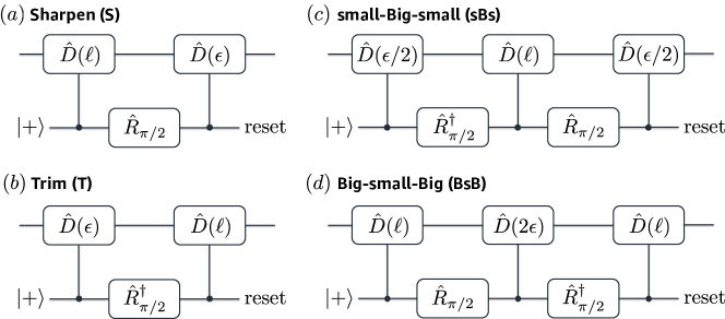
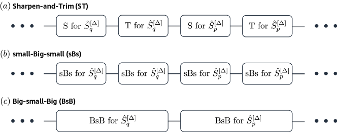
Here, we study the experimental feasibility of a highly squeezed GKP qunaught state with dB. Recall that the GKP squeezing dB is sufficient for achieving a low logical failure rate of the surface-GKP code with a small surface code distance (see Fig. 6b). There have been many theoretical proposals for preparing a finitely-squeezed GKP state [22, 57, 58, 59, 60, 61, 62, 63, 64, 65, 66, 67, 68, 69, 70, 38, 71]. In recent years, GKP qubits have been experimentally realized in trapped ion systems [23, 24, 26] as well as in a circuit QED system [25]. The achieved GKP squeezing in these experiments ranges from dB to dB. Notably, two of the recent experiments [25, 26] have used an autonomous (or dissipative) stabilization method, namely the Sharpen-and-Trim (ST) scheme [25] and the small-Big-small (sBs) scheme [26], to prepare and stabilize a finitely-squeezed GKP state by using an ancilla qubit. Note also that a recent theoretical work [38] has identified the ST scheme as a first-order Trotter method and proposed two new methods, small-Big-small (sBs) and Big-small-Big (BsB) schemes, by using the second-order Trotter formula (see Fig. 8; the sBs scheme is also independently discovered in Ref. [26]).
In this section, we demonstrate that the BsB scheme is particularly well suited for preparing a highly squeezed GKP qunaught state (with a GKP squeezing dB) in the presence of realistic imperfections such as photon loss and ancilla qubit decay and dephasing. We also propose a modification of the existing schemes by using a three-level ancilla instead of a two-level ancilla qubit. More specifically, we show that the stabilization schemes can be made robust against single ancilla decay events by using a three-level ancilla with a properly engineered conditional displcement operation. In particular, we demonstrate that a highly squeezed GKP qunaught state of GKP squeezing dB can in principle be realized in circuit QED systems assuming reasonable experimental parameters.
IV.1 Dissipative preparation of a GKP qunaught state
Given the optimal performance of the square-lattice GKP code in the surface-GKP code as demonstrated in Fig. 7, we focus on stabilizing the square-lattice GKP qunaught state. Let be the ideal, infinitely-squeezed square-lattice GKP qunaught state. A finitely-squeezed GKP qunaught state (with a Gaussian envelope) is given by . Here, approximately equals the noise variance of the finitely-squeezed GKP state, i.e., (see Section A.3 for more details). Note that the finitely-squeezed GKP qunaught state is only approximately stabilized by the stabilizers of the infinitely-squeezed GKP qunaught state and . However, as observed in Ref. [38], it is possible to define exact stabilizers of a finitely-squeezed GKP state. For instance, the finitely-squeezed GKP qunaught state is exactly stabilized by the following stabilizers:
| (35) |
In two recent experiments [26, 25], these stabilizers are stabilized by using the Sharpen-and-Trim (ST) method shown in Fig. 8 (a) and (b). The two new schemes proposed in Ref. [38], namely the sBs and BsB schemes, are shown in Fig. 8 (c) and (d), respectively. Note that unlike phase estimation methods [61, 65], the dissipative schemes in Fig. 8 do not require active monitoring of the ancilla qubit state and real-time feedback control based on the ancilla measurement outcome. Instead, it suffices to simply reset the ancilla qubit to regardless of the ancilla state at the end of the circuit.
Every scheme in Fig. 8 requires conditional displacement operations and (or or ), single-qubit rotations and , and the ancilla qubit reset (to the state). Here, the conditional displacement operator is defined as and the single-qubit rotation is defined as , where and . To stabilize (i.e., position quadrature), we choose and . Also, to stabilize (i.e., momentum quadrature), we choose and .
To prepare and stabilize a finitely-squeezed GKP qunaught state, we start from the vacuum state and apply multiple rounds of the disspative stabilization circuits in Fig. 8. The exact sequence of the stabilization is shown in Fig. 9. Each sequence consists of stabilization of the position quadrature which is followed by stabilization of the momentum quadrature. In the case of the sBs scheme, we observe that a GKP qunaught state cannot be properly prepared from the vacuum state if the position (momentum) stabilization is not repeated at least twice. Thus, we choose to repeat the stabilization of each quadrature twice before moving on to the stabilization of the other quadrature (see Fig. 9 (b)). Note also that each BsB scheme contains two big conditional displacements (), whereas all the other schemes (i.e., S, T, sBs) contain only one big conditional displacement. Thus, if the conditional displacement is the slowest process, each BsB scheme takes twice as long as the other schemes.
Note that we can freely choose the parameter which determines the size (and thus squeezing) of the output GKP state. Since and the noise variance of the finitely-squeezed GKP state are approximately identical to each other in the (or high squeezing) regime, we define the target GKP squeezing analogously as in Eq. 17. Hence, given the target GKP squeezing , we choose to be
| (36) |
Then, suppose that the stabilization circuit outputs a state . Unlike in Ref. [38] where the goal was to stabilize a GKP qubit, we only aim to stabilize a finitely-squeezed GKP qunaught state. Hence, there is no notion of logical qubit fidelity, which was the main focus of the study in Ref. [38], because there is no logical information encoded in the GKP qunaught state. Instead, we are only interested in how much the output GKP qunaught state is squeezed in both the position and the momentum quadratures. Thus, similarly as in Refs. [45, 72], we define the effective GKP squeezings (in position and momentum quadratures) of the state as follows and use them as the key figure of merit:
| (37) |
Here, and . This definition of the GKP squeezing is motivated by the following observation.
| (38) |
That is, one can infer the effective noise variance from the expectation values of the stabilizers and (of the infinitely-squeezed GKP qunaught state) and then convert them into the unit of decibel as in Eq. 37.
IV.2 Performance of the dissipative preparation methods
IV.2.1 Ideal ancilla qubit
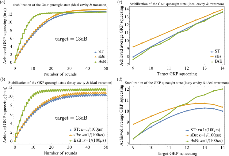
We now show the performance of the three dissipative GKP-state preparation methods (i.e., ST, sBs, and BsB). For now, we consider an ideal case where the ancilla qubit (e.g., transmon) is noiseless. In Fig. 10 (a) and (b), we show the achieved GKP squeezing (in the position quadrature, i.e., ) as a function of the number of rounds, starting from the vacuum state . In particular, we set the target GKP squeezing to be dB. With the circuit QED system in mind, we refer to the bosonic mode (where the GKP state is prepared) as a cavity and the ancilla qubit as a transmon. To demonstrate that all three schemes (ST, sBs, BsB) achieve the intended goal, we assume that the cavity mode and the transmon are noiseless in Fig. 10 (a). In this case, after sufficiently many rounds of stabilization, the ST, sBs, and BsB schemes output a finitely-squeezed GKP qunaught state with an effective GKP squeezing of dB, dB, and dB, respectively. Notably, the BsB scheme reaches the steady state configuration with the fewest number of stabilization rounds.
Then, we consider the adverse effects of photon loss in the cavity mode and transmon relaxation and dephasing. In particular, we focus on the effects of photon loss and transmon errors that occur during the conditional displacement operations. That is, while we assume that single-qubit rotations are noiseless and instantaneous, we simulate the conditional displacement operations via a Lindblad master equation
| (39) |
where or and we assume . Here, is the annihilation operator of the cavity mode and is the annihilation operator of the ancilla transmon, i.e., . For now, we assume that the ancilla transmon is free from relaxation and dephasing to understand the limitations imposed by the non-zero photon loss rate .
In Fig. 10 (b), we take and . In this case, the achieved GKP squeezings in the final steady state configuration are given by dB, dB, and dB for ST, sBs, and BsB schemes, respectively. The temporary drop in the output GKP squeezing (e.g., in the position quadrature) is due to the photon loss during the stabilization of the other quadrature (e.g., the momentum quadrature). Note that the BsB scheme is most resilient against the cavity photon loss as it experiences a decrease in the achieved GKP squeezing by only dB whereas the ST and sBs schemes see a decrease by about dB.
In Fig. 10 (c) and (d), we vary the target GKP squeezing from dB to dB and study the saturated value of the GKP squeezing as a function of the target GKP squeezing. Simiarly as in Fig. 10 (a), we assume that both cavity and transmon are noiseless in Fig. 10 (c). In this case, not so surprisingly, the achieved GKP squeezing increases as we increase the target GKP squeezing. This is not necessarily the case, however, when the cavity mode suffers from photon loss. As shown in Fig. 10 (d), if the cavity photon loss rate is given by (which should be compared with ), the achieved GKP squeezing peaks at a certain value of the target GKP squeezing. For instance, the maximum achievable GKP squeezing with the ST scheme is given by dB which is achived when the target GKP squeezing is dB. Similarly, the optimal performance of the sBs scheme is achieved when the target GKP squeezing is dB with which a GKP squeezing of dB is achieved. The existence of a peak is due to the fact that, given the same coupling strength for the conditional displacement operation, the effective stabilization rate decreases as we increase the target GKP squeezing (see Ref. [38] for more details), whereas the photon loss rate remains constant.
In the case of the BsB scheme, the achieved GKP squeezing continues to increase as we increase the target GKP squeezing from dB to dB. In particular, a GKP squeezing of dB can be achieved by setting the target GKP squeezing to be dB. We expect, however, that the achieved GKP squeezing will eventually peak at a certain value of the target GKP squeezing just like in the case of the ST and sBs schemes for the reason described above.
The result in Fig. 10 (d) has an important implication: even if the ancilla transmon is assumed to be noiseless, the maximum achievable GKP squeezing is eventually limited by the photon loss rate in proportion to the coupling strength for the conditional displacement operations. Hence, regardless of whether we mitigate the ancilla transmon errors (which we will discuss shortly), the GKP squeezing cannot be made arbitrarily large under a non-vanishing photon loss rate. Nevertheless, the BsB scheme is shown to be most robust against photon loss errors and achieves a GKP squeezing of dB assuming realistic parameters for the coupling strength and the photon loss rate . Thus, we mainly focus on the BsB scheme from now on.
IV.2.2 Noisy ancilla qubit
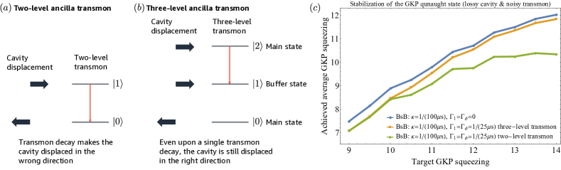
We now consider the adverse effects due to transmon decay and dephasing. As previously noted in Ref. [38], ancilla transmon dephasing does not limit the performance of all three stabilization methods (i.e., ST, sBs, BsB methods). This is because the transmon dephasing commutes with the conditional displacement operations and hence does not cause any undesired displacement in the cavity mode. However, transmon decay can significantly compromise the performance of the GKP state stabilization methods. This is because transmon decay in the middle of a conditional displacement operation can cause a large undesirable shift to the cavity mode. That is, if the transmon decays from to during a conditional displacement (generated by or ), the cavity state is displaced in wrong direction, possibly by a large amount depending on when the transmon decayed (see Fig. 11 (a)). Indeed, as shown in Fig. 11, if the transmon decay and dephasing rates are given by and the cavity photon loss rate is , the achievable GKP squeezing is significantly lower (dB) compared to the case when the cavity photon loss rate remains the same but the transmon is assumed to be noiseless (dB).
Here, to mitigate the adverse effects of transmon decay, we propose to use the third level of the ancilla transmon. That is, we propose to use the ground state and the second excited state of the transmon as the main ancilla qubit basis states. Thus, for instance, the ancilla transmon is initialized to a state instead of . Also, the single-qubit rotation is replaced by , and the annihilation operator of the ancilla transmon is replaced by (note that we are thus assuming the second excited state of the transmon decays twice faster than the first excited state). The key feature of this three-level ancilla scheme is to use the first excited state of the transmon as a buffer state for possible single transmon decay events (from to ). Most importantly, to make sure that the cavity mode is displaced in the right direction by the same amount even upon a single transmon decay, we carefully engineer the conditional displacement operation and propose to realize it via the following Hamiltonian
| (40) |
or . In this case, even if the second excited state of the transmon decays to its first excited state , the above Hamiltonian still generates the same displacement in the cavity mode. Thus, regardless of when the transmon decays from to , the cavity mode is still displaced by or (relative to the case where the transmon is in the ground state ) which is approximately equal to , hence a trivial shift to the square-lattice GKP qunaught state. However, in a much less likely event where the transmon experiences two decay events (), the cavity mode may be shifted by an undesirable amount, leading to an increased noise variance in the output GKP qunaught state. Note that the design principle behind the interaction in Eq. 40 is also related to the ideas of error transparency [73, 74, 75, 76] and path independence [77].
The effectiveness of the three-level transmon scheme is demonstrated in Fig. 11 (c). As indicated by the orange line, despite the strong transmon decay and dephasing rates , the three-level transmon scheme nearly achieves as high GKP squeezing as in the case where the transmon is assumed to be noiseless (i.e., blue line). In particular, while the two-level transmon scheme can only achieve a GKP squeezing of dB at most, the three-level scheme can achieve a GKP squeezing of dB choosing the target GKP squeezing to be dB. Moreover, it can potentially realize a higher GKP squeezing by further increasing the target GKP squeezing.
Thus, we show that a highly squeezed GKP qunaught state of GKP squeezing dB can in principle be achieved via the BsB scheme with reasonable experimental parameters , , and by using the three-level transmon scheme. Note that if the transmon relaxation time is longer, the third level of the transmon may not be needed and the two-level transmon scheme may suffice to reach the ultimate limit set by . For instance, if the photon loss rate and the transmon dephasing rates remain the same ( and ) but the transmon decay rate is smaller (), the two-level transmon scheme achieves a GKP squeezing of dB, close to the limit dB set by the photon loss, by choosing the target GKP squeezing to be dB.
V Discussion and outlook
In this work, we delivered three main results: first, we introduced a maximum likelihood decoding for correcting shift errors in two-qubit gates between GKP qubits and showed that it significantly outperforms the simple closest-integer decoding scheme (see Table 1). Secondly, using space-time correlated edges in the matching graphs of the surface code decoder, we carefully took into account all types of errors arising from every error-corrected two-GKP-qubit gates throughout the full syndrome history. By doing so, we were able to achieve a low logical failure rate of the surface-GKP code with only moderate hardware requirements and a reasonable GKP squeezing dB (see Fig. 6b and Table 3). Lastly, we demonstrated that a highly-squeezed GKP state of GKP squeezing dB can in principle be realized by a dissipative stabilization method, namely the Big-small-Big method, with reasonable experimental parameters. In particular, we showed that the ancilla decay errors can be effectively mitigated through a suitably engineered three-level ancilla in the dissipative stabilization scheme.
Several remarks are in order. Recall that throughout the analysis of the surface-GKP code, we made a twirling approximation and treated the shift errors due to finite GKP squeezing as incoherent random shift errors. This is mostly for simulation purposes and it is not desirable to physically implement the shift twirling. This is because the shift twirling increases the energy of an encoded GKP state, making it susceptible to uncontrolled non-linear interactions. Thus, to have a refined understanding of the realistic, finitely-squeezed GKP qubits, one needs to analyze them without making the twirling approximation and instead assuming coherent shift errors. A recently proposed subsystem decomposition method [78] has shown to be useful for analyzing finitely-squeezed GKP states exactly [79, 80, 81]. In this work, however, we have not performed such an analysis partly because one would then get a generic noise channel for a GKP qubit after each GKP error correction. In this case, the Gottesman-Knill simulation methods [82, 83] no longer apply in the analysis of the surface code. As such, large-distance surface codes could not be simulated efficiently using the exact noise model for finitely squeezed GKP states. Nevertheless, analyzing the effects of the coherence is still an important task and we leave it as a future work. Related to this, we remark that recent work, which uses a teleportation-based GKP error correction protocol which is similar to the one presented in this manuscript, has demonstrated that approximate results based on shift twirling agree well with the exact numerical results. The results apply to the single GKP qubit setting [84].
Recall that we have neglected photon loss and heating since finite squeezing of the GKP qunaught states is the dominant source of error (at least in the near term). The addition of other noise sources such as photon loss and heating will modify the shift distribution and correlation structure. Hence, maximum-likelihood decoding for two-GKP-qubit gates should be adapted to the new shift distribution. Similarly, edge weights in the surface-code matching graphs should also be adjusted to account for modified conditional probabilities of various error types.
Note also that in this work we focused on fault-tolerant quantum error correction for building a logical quantum memory and have not discussed schemes for universal fault-tolerant quantum computation. Since we conclude that biasing the noise of the GKP qubits does not offer significant advantages in reducing the logical error rate (especially for the data qubits which will be used for carrying out the computation), the Toffoli magic state preparation schemes [20] and piece-wise fault-tolerant Toffoli gates [17, 19] that are tailored to noise-biased qubits would be sub-optimal for GKP encoded qubits. A more promising avenue would be to pursue the more widely used -type magic states [85]. In doing so, we can take advantage of the fact every operation between GKP qubits is error corrected and thus comes with extra analog information that can be used to determine the reliability of the gate. Hence, an interesting research direction is to see if the direct, fault-tolerant -type magic state preparation schemes in Ref. [86, 87] (which use flag-qubit techniques [88, 89, 90, 91, 92, 93, 94, 95] and redundant ancilla encoding) can be combined with the GKP qubits to significantly reduce the resource overheads for fault-tolerant quantum computing compared to the cases where bare two-level qubits are used. We also remark that a different decoder other than the MWPM decoder may be used in analyzing such fault-tolerant computing schemes to either reduce logical failure rates further (e.g., by using a tensor-network decoder [96, 97]) or to speed up the decoding at the expense of decreased performance (e.g., by using a Union Find decoder [98, 99, 100]).
Regarding the experimental realization of the GKP qubits, we emphasize that for the scope of this work, we only focused on achieving a high GKP squeezing dB and have not considered how long it takes to prepare such a highly-squeezed GKP state. In particular, the dissipative stabilization schemes, including the Big-small-Big scheme, require tens of stabilization rounds to prepare a GKP state from the vaccum state (corresponding to a preparation time assuming the coupling strength of the conditional displacement is ). Such long preparation times can potentially be problematic because it increases the idling time and hence makes the data qubits of the surface-GKP code susceptible to photon loss. Alternatively, idling times can be reduced by using more than two modes for each GKP qubit in a (teleportation-based) GKP error correction protocol. This is due to the fact that a subset of modes can begin preparing a GKP qunaught state well before it needs to be supplied to the circuit. In this case, the total number of oscillator modes will be larger than simply three times the number of GKP qubits in the surface-GKP code. As such, reducing the GKP state preparation time is important to maintain the hardware resource estimates obtained in this work.
One possible way to speed up the GKP state preparation protocol is to increase the coupling strength of the conditional displacement operations by driving the cavity [25] or transmon qubit [101] more strongly. The state preparation protocol can also be accelerated by starting from a squeezed state in one quadrature (e.g., ) [23, 24, 26] instead of the vacuum state so that we can mostly focus on squeezing the other quadrature (e.g., ). Also, it is important to realize that the dissipative stabilization method we considered in this work (e.g., the Big-small-Big scheme) does not utilize information gained by transmon as it is a completely autonomous process (see Fig. 8). However, there are other methods, namely phase estimation methods, that do take advantage of information gained by transmon [61, 65]. In this case, fewer rounds of measurements will be needed to achieve a high GKP squeezing with the help of feedback control based on the transmon measurement outcomes. As shown in Ref. [65], however, transmon measurement errors should be carefully post-processed via a majority-voting type of scheme. This is due to the fact that an incorrect feedback based on a single faulty measurement outcome can cause a large shift error and hence introduce extra noise thereby destroying the desired fault-tolerant properties of the state-preparation protocol.
We note that a long state preparation time will not be a limiting factor if the cavity lifetime is given by instead of : at the GKP squeezing dB, the noise variance due to the finite GKP squeezing is given by . If the state preparation time is and the cavity lifetime is , an additional noise variance (comparable to ) is introduced. However, if the cavity lifetime is , the extra noise variance is reduced to and is not appreciable compared to the noise variance due to the finite GKP squeezing.
Note also that we only considered preparation of a GKP qunaught state via an auxiliary qubit. Thus if we want to prepare a GKP-Bell state, which is needed for the teleportation-based GKP error correction, two GKP qunaught states have to be prepared sequentially using the same auxiliary qubit and then a beam-splitter interaction should be applied to them to turn them into a GKP-Bell state. In principle, this procedure can be simplified as we can use an auxiliary qubit to directly prepare a GKP-Bell state. More specifically, instead of measuring the two stabilizers of a GKP qunaught state for each mode, we can measure the four stabilizers of a GKP-Bell state jointly on the two modes. We leave a more detailed study of such a direct GKP-Bell state preparation as a future work.
Lastly, we remark that reducing the strength of non-linear interactions is especially crucial when working with highly-squeezed GKP states since these highly-energetic states are susceptible to non-linear interactions such as the self-Kerr and cross-Kerr interactions. In circuit QED systems, non-linear interactions have been minimized by coupling the cavity mode (where the GKP state resides in) much more weakly to an ancilla transmon than in the standard regime [25]. The desired conditional displacement operation is then selectively enhanced either by driving the cavity mode [25] or the transmon [101]. To go beyond preparing a single GKP state and be able to manipulate many GKP qubits, it is also essential to couple cavity modes via Gaussian operations. In circuit QED systems, Gaussian operations between cavity modes have been realized by using a four-wave mixing element [42, 43, 44]. In the context of manipulating GKP qubits, however, it is more desirable to use a three-wave mixing element (e.g., SNAIL [102] or ATS [16]) such that higher-order non-linear interactions are minimized. A holistic and detailed architecture analysis incorporating all these considerations, including the effects of photon loss, is left as a future work.
Acknowledgments
We would like to acknowledge the AWS EC2 resources which were used for part of the simulations performed in this work.
Appendix A GKP error correction
In this appendix, we derive Eqs. 8 and 15, i.e., ideal post-measurement state after a Steane-type and a teleportation-based GKP error correction, respectively. We also discuss how the envelope operators of finitely-squeezed ancilla GKP states propagate during a teleportation-based GKP error correction.
A.1 Steane-type GKP error correction
The Steane-type GKP error correction scheme can be decomposed into two stages. In the first stage, the GKP qubit in the second mode (prepared in the ) measures the position of the data mode modulo . Let be the input state in the data mode. After applying the SUM gate , we get
| (41) |
where we used
| (42) |
Then, conditioned on measuring in the second mode via a position homodyne measurement, we get
| (43) |
where the projection operator is given by
| (44) |
where the sign of the integer is flipped for a cosmetic reason without changing the results. Note that projects an input state to the space of states that have modulo .
In the second stage, the GKP qubit in the third mode (prepared in ) measures the momentum of the data mode modulo . This time, we expand the state in the data mode in the momentum basis, i.e., . Then, after applying the inverse SUM gate , we get
| (45) |
where we used
| (46) |
Thus, similarly as above, the post-measurement state upon measuring is given by
| (47) |
where
| (48) |
is the projection operator to the space of states that have modulo .
Combining Eqs. 43 and 47, we find that the ideal output state after the Steane-type GKP error correction is given by
| (49) |
Thus, to derive Eq. 8, it remains to show
| (50) |
Note that
| (51) |
where we used and the convention (see the caption of Fig. 1). Carrying on, we find
| (52) |
Lastly, since
| (53) |
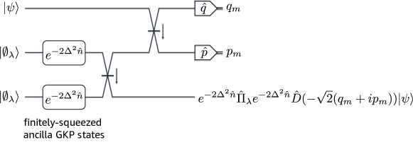
A.2 Teleportation-based GKP error correction
Recall that the teleportation-based GKP error correction is based on beam-splitter interactions. Under the beam-splitter interaction , position eigenstates are transformed as follows:
| (54) |
Applying the balanced beam-splitter interaction to two GKP qunaught states, we get a GKP-Bell state.
| (55) |
Then, applying a balanced beam-splitter interaction to , we find
| (56) |
and hence
| (57) |
Thus, after measuring and via homodyne measurements, we get
| (58) |
Carrying on, we obtain the desired result in Eq. 15:
| (59) |
A.3 Finitely-squeezed ancilla GKP states
A finitely-squeezed GKP state can be understood as a state resulting from applying a Gaussian envelope operator to an ideal GKP state. As shown in Ref. [30], the envelope operator can also be expressed as a coherent superposition of Gaussian shift errors, i.e.,
| (60) |
where and
| (61) |
For instance, a finitely-squeezed GKP qunaught state is given by
| (62) |
At the continuous-variable level, we can apply random shifts with random integers and , and convert the coherent Gaussian shifts into incoherent Gaussian shifts, i.e.,
| (63) |
if . See Appendix A in Ref. [30] for derivation. In our simulation, we use this incoherent shift noise model because otherwise the simulation cannot scale to large system sizes.
In realistic experimental setups, however, it is not desirable to physically implement the random shifts with random integers and because it will increase the energy of the encoded GKP states. Thus, it is also important to understand the outcome of teleportation-based GKP error correction with finitely-squeezed ancilla GKP states without making the twirling approximation. Note that the product of Gaussian envelope operators and commutes with the balanced beam-splitter interaction . Thus, after the balanced beam-splitter interaction , we have a finitely-squeezed GKP-Bell state Following the same derivation in Section A.2, we then find (see Fig. 12)
| (64) |
See also Ref. [40]. Due to the Gaussian envelope operator after the projection , the output state is guaranteed to be in the finitely-squeezed GKP code space and hence have a bounded energy. If we are not concerned about the energy of the state and are only interested in shift errors, the action of the envelope operator can be understood as the post-measurement shifts and shown in Fig. 2 (b). Similarly, another envelope operator before the projection guarantee that the measurement outcomes and are finite whenever the input state has a bounded energy. However, if we are only interested in the shift errors, this envelope operator can be understood as the pre-measurement shifts and shown in Fig. 2 (b).
Appendix B Maximum likelihood decoding of the logical two-qubit gates between two GKP qubits
Recall the optimization problem in Eq. 30:
| (65) |
given and . To solve this optimization, we tackle a closely related but slightly different problem: That is, we seek to find conditions on and such that is given by . Define as
| (66) |
Then, for and to have as the solution of the above optimization problem, they must satisfy
| (67) |
These conditions are reduced to
| (68) |
| (69) |
and
| (70) |
One can verify that other conditions such as are trivially satisfied if these three conditions hold. Thus, we can define Voronoi cells as follows:
| (71) |
Thus, to solve the optimization problem in Eq. 30, we can simply ask in which Voronoi cell lies in. This can be efficiently done by using Algorithm 1.
Similarly for the other optimization problem in Eq. 33 for the momentum quadratures, i.e.,
| (72) |
given and , we can identify the set of for which the solution is given by by imposing the following conditions:
| (73) |
where is defined as
| (74) |
In this case, the right hand side of the third condition is given by , instead of . This is related to the fact that the momentum noise and are negatively correlated. The corresponding Voronoi cells are given by
| (75) |
Hence, the optimization problem in Eq. 33 can be solved by finding in which Voronoi cell is in. This search can be efficiently done by using Algorithm 2. Note that the decision boundaries defined by the Voronoi cells in Eqs. 71 and 75 are visualized in Fig. 4 (c).
Appendix C Simulation details
In Section C.1, we discuss the noise model used in our surface-GKP code simulation. We also explain how compute the conditional failure probabilities of various circuit elements based on extra analog information obtained during GKP error corrections. Then, in Section C.2, we describe how the edge weights in the surface-code matching graphs are dynamically computed by using the conditional failure probabilities of circuit elements.
C.1 Noise model
Here, we discuss how to simulate state preparation, Pauli measurement, idling, CNOT, and CZ gates of the GKP qubits which are necessary to implement the surface-GKP code.
C.1.1 state preparation
To prepare a state in an ancilla mode of the surface-GKP code, we assume that the ancilla mode is initially prepared in a squeezed state, close to a momentum eigenstate . In particular, we assume that the variance of the momentum quadrature is given by . We then apply (noisy) teleportation-based GKP error-correction by using finitely-squeezed GKP qunaught states with the same noise variance . Since the GKP error correction is noisy due to the finite GKP squeezing, a momentum noise of variance is added to the ancilla mode (see Fig. 3 (b)). Then the net momentum noise variance is given by .
Hence, we simulate the state preparation as follows: we first sample a random shift from the Gaussian distribution of zero mean and variance . Then, compute an integer
| (76) |
Then, if is even (i.e., ), assume that is correctly prepared. On the other hand, if is odd (i.e., ), apply a Pauli error, or equivalently, assume that is prepared instead of .
To compute the edge weights in the matching graphs of the surface code, we need to know the failure probability of the state preparation. In the case where we ignore the extra analog information, we simply set to be the probability of being odd:
| (77) |
In practice, for the parameters we consider in this work (), it suffices to approximate by .
On the other hand, if the analog information is utilized, we first compute
| (78) |
Then, given this analog information, we compute the conditional probability as
| (79) |
where and are given by
| (80) |
Similarly as in the no-analog information case, it suffices to approximate by and by .
C.1.2 Pauli measurement
To simulate the Pauli measurement of an ancilla qubit of the surface-GKP code (which is encoded in a rectangular-lattice GKP code with ), we assume that it follows a noisy GKP error correction. This is because all Pauli measurements are preceded by an error-corrected two-qubit gate between two GKP qubits which ends with a noisy GKP error correction. Thus, the ancilla GKP qubit inherits a momentum shift from the noisy GKP error correction (see Fig. 3 (b)) before it is measured in the basis. The Pauli measurement itself is performed via a momentum homodyne measurement which we assume to be noiseless for simplicity. Assuming that the resolution of the homodyne measurement is not much worse than the noise standard deviation of the GKP qunaught states, the errors in the two-qubit gates (to be discussed below) are the dominant noise sources in the surface-GKP code. Thus, if this is the case, how precisely we model the homodyne measurement does not make an appreciable overall impact to the performance of the surface-GKP code.
Under this noise model, the rest of the noise simulation goes similarly as in the case of the state preparation. We first sample a random shift from the Gaussian distribution and compute an integer as follows:
| (81) |
If , we assume that the measurement is performed faithfully. If , however, we assume that the Pauli measurement is preceded by a Pauli error, i.e., the measurement outcome is flipped.
Then, we compute the probability (or conditional probability) of having a measurement error. If we ignore the analog information, we simply compute the probability of being odd:
| (82) |
where suffices in practice for .
On the other hand, if we exploit the extra analog information, we compute
| (83) |
and then set the conditional probability to be
| (84) |
where and are given by
| (85) |
Again, it suffices to use instead of and instead of .
C.1.3 Idling
The idling scenario is already discussed in great detail in Section II.2. To briefly remind ourselves, we assume that an idling is always preceded by a noisy GKP error correction and thus the idling mode inherits position and momentum shifts of noise variance from the previous noisy GKP error correction. At the end of the idling, another noisy GKP error correction is performed and hence extra position and momentum shifts errors of the same variance are added (see Fig. 2 (b)). Hence, the noise variance of the net accumulated position and momentum shift errors is given by .
Thus, to simulate an idling event, we first sample position and momentum shifts and independently from the Gaussian distribution , i.e., . Then, compute the two integers
| (86) |
For the idling locations in the data qubits of the surface-GKP code, we always use but for the ancilla qubits, we use . With these two integers and , we apply
| (87) |
and then apply
| (88) |
We then need to compute the probabilities (or conditional probabilities) of the idling Pauli errors, which are used to compute the edge weights in the matching graphs of the surface code. In the case where we do not use the extra analog information, we compute
| (89) |
and set to be
| (90) |
When the extra analog information is used, we first find
| (91) |
and then compute and as follows:
| (92) |
where are given by
| (93) |
Then, the conditional Pauli error probabilities are computed in the same way as in Eq. 90. Again, in practice, one can replace by and by in the parameter range .
C.1.4 CNOT
The detailed setup of the error-corrected CNOT gate between two GKP qubits is discussed in great detail in Section II.3. Here, we focus on describing how to simulate the CNOT gate. Note that the first qubit is the control qubit encoded in the rectangular-lattice GKP code and the second qubit is the target qubit encoded in the square-lattice GKP qubit.
First, we sample eight random shifts independently from the same Gaussian distribution , i.e., . Then, set as follows (see Eq. 25):
| (94) |
Then, given , compute two integers by using Algorithm 1 (by setting the inputs to be , instead of ). Similarly, given , compute two other integers by using Algorithm 2 with as an input instead of .
Given four integers , we apply
| (95) |
and then apply
| (96) |
Then, we need to compute Pauli error probabilities (or conditional probabilities) ,, which are used to determine the edge weights in the surface code matching graphs. If we do not use the extra analog information, we simply compute
| (97) |
where the integration domain is defined as
| (98) |
and the probability density function is given by
| (99) |
Similarly for the momentum shift errors, we compute
| (100) |
where the integration domain is defined as
| (101) |
and the probability density function is given by
| (102) |
Then, the Pauli error probabilities are given by
| (103) |
On the other hand, if we take into account the extra analog information, we define
| (104) |
and then compute
| (105) |
where are given by
| (106) |
Similarly, for the momentum shift errors, we compute
| (107) |
where are given by
| (108) |
Then, the conditional Pauli error probabilities are computed by using Eq. 103. In practice, , , , and can be replaced by , , , and , respectively.
C.1.5 CZ
We consider an error-corrected CZ gate between two GKP qubits (see Fig. 3 (d)). We assume that the first qubit is encoded in the rectangular-lattice GKP code and the second qubit is encoded in the square-lattice GKP qubit. Thus, unlike the usual CZ gate, there is no permutation symmetry unless the first qubit is also encoded in the square-lattice GKP code.
To simulate the CZ gate, we first sample eight random shifts independently from the Gaussian distribution , i.e., and set
| (109) |
Note that is correlated with and is correlated with . First, given , we need to find two integers such that is in the Voronoi cell , where is defined as
| (110) |
This is done in the exactly the same way as in Algorithm 1.
Similarly, given , we need to find two other integers such that is in the Voronoi cell , where is defined as
| (111) |
This can be done by using a slightly modified version of Algorithm 2 with proper sign changes.
Similarly as in the case of the CNOT gate, given four integers , we apply
| (112) |
and then apply
| (113) |
Then, in the case where we neglect the extra analog information, we compute
| (114) |
and
| (115) |
to get the Pauli error probabilities
| (116) |
Here, the probability density functions and are defined as
| (117) |
and
| (118) |
If we use the extra analog information, we define
| (119) |
and then compute
| (120) |
where are given by
| (121) |
Similarly, we also compute
| (122) |
where are given by
| (123) |
Then, the conditional Pauli error probabilities are computed by using Eq. 116. In practice, , , , and can be replaced by , , , and , respectively.
C.2 Edge weights in the matching graphs
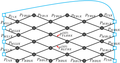
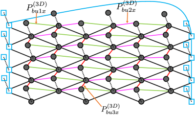
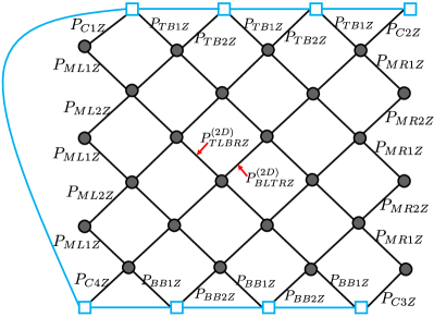
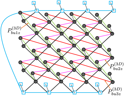
In this section we describe the methods used to perform the simulations of the surface-GKP code for various code distances. As a first step, in Fig. 13, we illustrate the matching graphs used in the implementation of the MWPM algorithm with weighted edges. Two-dimensional bulk and boundary edges are distinguished by their associated labels since such edges will have different weights. Vertical edges used for detecting measurement errors (see Ref. [5]) are dashed. Lastly, consider the space-time correlated edges in Figs. 13b and 13d used for detecting errors arising from CNOT/CZ failures which result in errors with a spatial and temporal component (see Refs. [103, 92, 93, 20]). Such edges are distinguished by their labels and associated colors. For instance, space-time correlated edges colored in green in Fig. 13b are labelled .
We now describe how to compute the weights for edges in the matching graphs of Fig. 13. As shown in Section C.1, if the extra analog information from GKP error corrections is used, the conditional probabilities for the failure rates of each circuit component is computed dynamically for every gate, idle, state-preparation and measurement location at each time step. As such, all circuit components can have different conditional probabilities at every location and in each syndrome measurement round. Hence edge weights for the matching graphs cannot be pre-computed and must be updated dynamically.
Given the above, let be the number of syndrome measurement rounds for a surface with minimum weight logical operator and minimum weight logical operator . We define a matrix where , and . Here, is the number of syndrome measurement rounds, corresponds to the number of data qubits, corresponds to the number of -type stabilizers and corresponds to the number of -type stabilizers.
The matrix can be decomposed into blocks and each block can be decomposed into three sub-matrices where . The matrix is , is and is . We now describe the constituents of each sub-matrix for a given block.
The columns of the sub-matrix can be decomposed into blocks, where the ’th block stores the conditional probabilities for , and Pauli errors arising from idling fault locations on the ’th data qubit and in the ’th syndrome measurement round (ancilla qubits have no idling fault locations). Note that data qubits on the boundaries of the lattice can have more than one idling fault locations in a given syndrome measurement round (for instance, if three two-qubit gates interact with a data qubit with an idling location in between two gates). However, because we do not consider photon loss in this work, all idling fault locations can be set at the beginning of a syndrome measurement round and thus incorporates the measurement and reset wait time. As such, we can write
| (124) |
where for instance is the conditional probability of a Pauli error on the ’th data qubit during the ’th syndrome measurement round arising from an idling fault location.
The columns of can be decomposed into blocks, where the ’th block stores all conditional probabilities arising from fault locations on the ’th ancilla for -type stabilizer measurements during the ’th syndrome measurement round. We note that by default, we consider a fault location for a two-qubit gate be on the control-qubit of such a gate, and we set the control qubit af a CZ gate to be on the ancilla qubit. On a given ancilla qubit, there are 62 fault locations: one for the state preparation, one for the -basis measurement and each of the four two-qubit gates can fail introducing a two-qubit Pauli error (of which there are 15 non-trivial possibilities). Since the ordering is important for what follows, we define
| (125) |
where , corresponds to the ’th ancilla for -type stabilizers and corresponds to conditional probability for the error occurring on a CNOT gate in time-step during the ’th syndrome measurement round. Hence stores the conditional probabilities of all 15 two-qubit Pauli errors for the CNOT gate applied in time step during the ’th syndrome measurement round and which interacts with the ancilla . We note that for ancillas used in measuring a weight-two -type stabilizer, if no CNOT gates are applied in time step , we set all terms in Eq. 125 to zero. Using Eq. 125, we can write
| (126) |
where and are the conditional probabilities for state-preparation and measurement errors on the ’th ancilla qubit for -type stabilizer measurements. We also note that we use the convention where ancillas for -type stabilizers are labeled top-bottom and left to right in the surface code lattice shown in Fig. 5.
The columns of into blocks where the ’th block stores all conditional probabilities arising from fault locations on the ’th ancilla for -type stabilizer measurements during the ’th syndrome measurement round. We define the vector in the same way as in Eq. 125 but where the terms correspond to the conditional probability of a error accuring during a CZ gate in time step during the ’th syndrome measurement round. As such, we can write
| (127) |
where and are the conditional probabilities for state-preparation and measurement errors on the ’th ancilla qubit for -type stabilizer measurements.
From the above, we can then write the matrix as
| (128) |
where is computed using Eqs. 124, 126 and 127. After performing all syndrome measurement rounds and generating the matrix, edge weights are computed by extracting the appropriate terms in the matrix.
We now illustrate the methods to compute the edge weight for bulk edges labeled in Fig. 13a using the matrix formalism (edge weights for other edges can be computed in an analogous fashion). In what follows, we will refer to such an edge as .
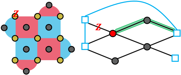
Let correspond to the data qubit represented by t. Upon looking at the circuit in Fig. 5, it can be seen that to leading order, the only fault locations which can result in being highlighted when implementing MWPM are failures on CNOT gates in the second and fifth time step of an -type stabilizer whose target qubit is . In addition, a or data qubit error during an idling location on can also result in to be highlighted. For the CNOT gate in the second time step, only errors from the set can contribute to being highlighted. Similarly, for the CNOT in time step 5, only errors from the set can contribute to being highlighted. Next we define the following functions:
| (129) |
| (130) |
and
| (131) |
Furthermore, let be the label for the ancilla qubit of an -type stabilizer where the CNOT gate in the second time step has as the target qubit. Define so that labels the ancilla qubit of an -type stabilizer where the CNOT gate in the fifth time step has as the target qubit. From Eq. 129, the ordering convention used in Eq. 125 and the construction of the matrix, the total probability of being highlighted from a failure of the CNOT gate in the second time step during the ’th syndrome measurement round is
| (132) |
where is the element in the ’th row of the matrix. Similarly, the total probability of being highlighted from a failure of the CNOT gate in the fifth time step during the ’th syndrome measurement round (assuming ) is
| (133) |
Note that in Eq. 133, the index for the syndrome measurement round is and not . This is because failures from the CNOT gate in the fifth time step add Pauli errors which are only detected in the next round. As such, this example highlights the importance of storing the conditional probabilities for the syndrome history and not just the conditional probabilities for the current syndrome measurement round.
The total probability of being highlighted from an idle failure on the data qubit during the ’th syndrome measurement round is
| (134) |
Using Eqs. 132, 133 and 134, the total probability to leading order for being highlighted during the ’th syndrome measurement round if is
| (135) |
If , we omit the term in Eq. 135. The edge weight for the edge is then
| (136) |
We conclude this section by noting that the function in Eq. 130 is used when fault locations arising from -type syndrome measurements must be taken into account when computing leading order edge weights.
C.3 Fault-tolerance properties of the surface-GKP code when using the analog information
In this section we show how a single fault in a distance-three surface-GKP code can result in a logical failure when taking into account the analog information for dynamically computing the edge weights of the matching graphs. To be clear, here we make an important distinction between faults and shift errors. A fault will always be taken to be an event such that after implementing the GKP error correction or performing a homodyne measurement, a non-trivial Pauli error is added to GKP qubits or a flip in the Pauli measurement outcome occurs.
In Fig. 14, we illustrate a case where a single fault results in a data qubit error on the first data qubit. Such a data qubit error results in the red highlighted vertex of the matching graph to the right of the figure. Typically, the minimum weight path would be to choose a single edge connecting the red highlighted vertex to a blue boundary vertex on the left-hand side of the matching graph. However, there are very rare cases where, after obtaining all conditional probabilities from the GKP error correction, the two edges highlighted in green in Fig. 14 will have a combined total weight which is less than either edge connecting the red highlighted vertex to a left boundary vertex. Further, such a scenario occurs even though no data qubit errors are present on the green highlighted edges. This is possible when, for instance, the two data qubits in these green highlighted edges have large but correctable shift errors. In this case, these shift errors are correctly inferred and countered (hence not causing a Pauli error). Nevertheless, they come with large conditional error probabilities (i.e., false alarm) because they are too close to the decision boundary that they could have been an uncorrectable shift which does result in a Pauli error. As such, when performing MWPM, the path highlighted in green in Fig. 14 will be chosen resulting in a logical fault.
The above example shows that when using the analog information to dynamically compute the edge weights of the matching graphs, edges which have no errors may nevertheless be favored by the MWPM algorithm (due to the false alarm as discussed above), thus making the MWPM decoder choose a wrong path when pairing highlighted vertices. However it is important to keep in mind that the probability of such events occurring is very small (for the example above at dB, we found such probabilities to be approximately whereas the logical error rate is ). Further, for larger code distances, higher order events need to occur such that fewer than faults resulting in non-trivial data qubit errors still lead to a logical failure. The probabilities of these higher order events are smaller than the computed logical failure rates and thus have a negligible contribution to the total logical failure rates in Fig. 6b. To conclude, incorporating the extra analog information provides an overall benefit despite the possible, but very rare, false alarms (compare Fig. 6a with Fig. 6b).
References
- Preskill [2018] J. Preskill, Quantum Computing in the NISQ era and beyond, Quantum 2, 79 (2018).
- Gottesman [2009] D. Gottesman, An Introduction to Quantum Error Correction and Fault-Tolerant Quantum Computation, arXiv e-prints , arXiv:0904.2557 (2009), arXiv:0904.2557 [quant-ph] .
- Shor [1994] P. W. Shor, Algorithms for quantum computation: discrete logarithms and factoring, in Proceedings 35th Annual Symposium on Foundations of Computer Science (1994) pp. 124–134.
- Lloyd [1996] S. Lloyd, Universal quantum simulators, Science 273, 1073 (1996).
- Fowler et al. [2012a] A. G. Fowler, M. Mariantoni, J. M. Martinis, and A. N. Cleland, Surface codes: Towards practical large-scale quantum computation, Phys. Rev. A 86, 032324 (2012a).
- Koch et al. [2007] J. Koch, T. M. Yu, J. Gambetta, A. A. Houck, D. I. Schuster, J. Majer, A. Blais, M. H. Devoret, S. M. Girvin, and R. J. Schoelkopf, Charge-insensitive qubit design derived from the cooper pair box, Phys. Rev. A 76, 042319 (2007).
- Schreier et al. [2008] J. A. Schreier, A. A. Houck, J. Koch, D. I. Schuster, B. R. Johnson, J. M. Chow, J. M. Gambetta, J. Majer, L. Frunzio, M. H. Devoret, S. M. Girvin, and R. J. Schoelkopf, Suppressing charge noise decoherence in superconducting charge qubits, Phys. Rev. B 77, 180502 (2008).
- Egan et al. [2020] L. Egan, D. M. Debroy, C. Noel, A. Risinger, D. Zhu, D. Biswas, M. Newman, M. Li, K. R. Brown, M. Cetina, and C. Monroe, Fault-Tolerant Operation of a Quantum Error-Correction Code, arXiv e-prints , arXiv:2009.11482 (2020), arXiv:2009.11482 [quant-ph] .
- Albert et al. [2018] V. V. Albert, K. Noh, K. Duivenvoorden, D. J. Young, R. T. Brierley, P. Reinhold, C. Vuillot, L. Li, C. Shen, S. M. Girvin, B. M. Terhal, and L. Jiang, Performance and structure of single-mode bosonic codes, Phys. Rev. A 97, 032346 (2018).
- Joshi et al. [2021] A. Joshi, K. Noh, and Y. Y. Gao, Quantum information processing with bosonic qubits in circuit qed, Quantum Science and Technology (2021).
- Cai et al. [2020] W. Cai, Y. Ma, W. Wang, C. L. Zou, and L. Sun, Bosonic quantum error correction codes in superconducting quantum circuits, arXiv e-prints , arXiv:2010.08699 (2020), arXiv:2010.08699 [quant-ph] .
- Cochrane et al. [1999] P. T. Cochrane, G. J. Milburn, and W. J. Munro, Macroscopically distinct quantum-superposition states as a bosonic code for amplitude damping, Phys. Rev. A 59, 2631 (1999).
- Jeong and Kim [2002] H. Jeong and M. S. Kim, Efficient quantum computation using coherent states, Phys. Rev. A 65, 042305 (2002).
- Mirrahimi et al. [2014] M. Mirrahimi, Z. Leghtas, V. V. Albert, S. Touzard, R. J. Schoelkopf, L. Jiang, and M. H. Devoret, Dynamically protected cat-qubits: a new paradigm for universal quantum computation, New Journal of Physics 16, 045014 (2014).
- Leghtas et al. [2015] Z. Leghtas, S. Touzard, I. M. Pop, A. Kou, B. Vlastakis, A. Petrenko, K. M. Sliwa, A. Narla, S. Shankar, M. J. Hatridge, M. Reagor, L. Frunzio, R. J. Schoelkopf, M. Mirrahimi, and M. H. Devoret, Confining the state of light to a quantum manifold by engineered two-photon loss, Science 347, 853 (2015), 1412.4633 .
- Lescanne et al. [2020] R. Lescanne, M. Villiers, T. Peronnin, A. Sarlette, M. Delbecq, B. Huard, T. Kontos, M. Mirrahimi, and Z. Leghtas, Exponential suppression of bit-flips in a qubit encoded in an oscillator, Nature Physics 16, 509 (2020).
- Guillaud and Mirrahimi [2019] J. Guillaud and M. Mirrahimi, Repetition cat qubits for fault-tolerant quantum computation, Phys. Rev. X 9, 041053 (2019).
- Puri et al. [2020] S. Puri, L. St-Jean, J. A. Gross, A. Grimm, N. E. Frattini, P. S. Iyer, A. Krishna, S. Touzard, L. Jiang, A. Blais, S. T. Flammia, and S. M. Girvin, Bias-preserving gates with stabilized cat qubits, Science Advances 6, 10.1126/sciadv.aay5901 (2020).
- Guillaud and Mirrahimi [2020] J. Guillaud and M. Mirrahimi, Error Rates and Resource Overheads of Repetition Cat Qubits, arXiv e-prints , arXiv:2009.10756 (2020), arXiv:2009.10756 [quant-ph] .
- Chamberland et al. [2020] C. Chamberland, K. Noh, P. Arrangoiz-Arriola, E. T. Campbell, C. T. Hann, J. Iverson, H. Putterman, T. C. Bohdanowicz, S. T. Flammia, A. Keller, G. Refael, J. Preskill, L. Jiang, A. H. Safavi-Naeini, O. Painter, and F. G. S. L. Brandão, Building a fault-tolerant quantum computer using concatenated cat codes, arXiv e-prints , arXiv:2012.04108 (2020), arXiv:2012.04108 [quant-ph] .
- Aliferis and Preskill [2008] P. Aliferis and J. Preskill, Fault-tolerant quantum computation against biased noise, Phys. Rev. A 78, 052331 (2008).
- Gottesman et al. [2001] D. Gottesman, A. Kitaev, and J. Preskill, Encoding a qubit in an oscillator, Phys. Rev. A 64, 012310 (2001).
- Flühmann et al. [2019] C. Flühmann, T. L. Nguyen, M. Marinelli, V. Negnevitsky, K. Mehta, and J. P. Home, Encoding a qubit in a trapped-ion mechanical oscillator, Nature 566, 513 (2019).
- Flühmann and Home [2020] C. Flühmann and J. P. Home, Direct characteristic-function tomography of quantum states of the trapped-ion motional oscillator, Phys. Rev. Lett. 125, 043602 (2020).
- Campagne-Ibarcq et al. [2020] P. Campagne-Ibarcq, A. Eickbusch, S. Touzard, E. Zalys-Geller, N. E. Frattini, V. V. Sivak, P. Reinhold, S. Puri, S. Shankar, R. J. Schoelkopf, L. Frunzio, M. Mirrahimi, and M. H. Devoret, Quantum error correction of a qubit encoded in grid states of an oscillator, Nature 584, 368 (2020).
- de Neeve et al. [2020] B. de Neeve, T. L. Nguyen, T. Behrle, and J. Home, Error correction of a logical grid state qubit by dissipative pumping, arXiv e-prints , arXiv:2010.09681 (2020), arXiv:2010.09681 [quant-ph] .
- Fukui et al. [2017] K. Fukui, A. Tomita, and A. Okamoto, Analog quantum error correction with encoding a qubit into an oscillator, Phys. Rev. Lett. 119, 180507 (2017).
- Fukui et al. [2018] K. Fukui, A. Tomita, A. Okamoto, and K. Fujii, High-threshold fault-tolerant quantum computation with analog quantum error correction, Phys. Rev. X 8, 021054 (2018).
- Vuillot et al. [2019] C. Vuillot, H. Asasi, Y. Wang, L. P. Pryadko, and B. M. Terhal, Quantum error correction with the toric gottesman-kitaev-preskill code, Phys. Rev. A 99, 032344 (2019).
- Noh and Chamberland [2020] K. Noh and C. Chamberland, Fault-tolerant bosonic quantum error correction with the surface–gottesman-kitaev-preskill code, Phys. Rev. A 101, 012316 (2020).
- Yamasaki et al. [2020] H. Yamasaki, K. Fukui, Y. Takeuchi, S. Tani, and M. Koashi, Polylog-overhead highly fault-tolerant measurement-based quantum computation: all-Gaussian implementation with Gottesman-Kitaev-Preskill code, arXiv e-prints , arXiv:2006.05416 (2020), arXiv:2006.05416 [quant-ph] .
- Fukui et al. [2020] K. Fukui, R. N. Alexander, and P. van Loock, All-Optical Long-Distance Quantum Communication with Gottesman-Kitaev-Preskill qubits, arXiv e-prints , arXiv:2011.14876 (2020), arXiv:2011.14876 [quant-ph] .
- Larsen et al. [2021] M. V. Larsen, C. Chamberland, K. Noh, J. S. Neergaard-Nielsen, and U. L. Andersen, A fault-tolerant continuous-variable measurement-based quantum computation architecture, arXiv e-prints , arXiv:2101.03014 (2021), arXiv:2101.03014 [quant-ph] .
- Bourassa et al. [2021] J. E. Bourassa, R. N. Alexander, M. Vasmer, A. Patil, I. Tzitrin, T. Matsuura, D. Su, B. Q. Baragiola, S. Guha, G. Dauphinais, K. K. Sabapathy, N. C. Menicucci, and I. Dhand, Blueprint for a Scalable Photonic Fault-Tolerant Quantum Computer, Quantum 5, 392 (2021).
- Rozpedek et al. [2021] F. Rozpedek, K. Noh, Q. Xu, S. Guha, and L. Jiang, Quantum repeaters based on concatenated bosonic and discrete-variable quantum codes, npj Quantum Information 7, 102 (2021).
- Xue et al. [2020] X. Xue, B. D’Anjou, T. F. Watson, D. R. Ward, D. E. Savage, M. G. Lagally, M. Friesen, S. N. Coppersmith, M. A. Eriksson, W. A. Coish, and L. M. K. Vandersypen, Repetitive quantum nondemolition measurement and soft decoding of a silicon spin qubit, Phys. Rev. X 10, 021006 (2020).
- D’Anjou [2021] B. D’Anjou, Generalized figure of merit for qubit readout, Phys. Rev. A 103, 042404 (2021).
- Royer et al. [2020] B. Royer, S. Singh, and S. M. Girvin, Stabilization of finite-energy gottesman-kitaev-preskill states, Phys. Rev. Lett. 125, 260509 (2020).
- Puri et al. [2019] S. Puri, A. Grimm, P. Campagne-Ibarcq, A. Eickbusch, K. Noh, G. Roberts, L. Jiang, M. Mirrahimi, M. H. Devoret, and S. M. Girvin, Stabilized cat in a driven nonlinear cavity: A fault-tolerant error syndrome detector, Phys. Rev. X 9, 041009 (2019).
- Walshe et al. [2020] B. W. Walshe, B. Q. Baragiola, R. N. Alexander, and N. C. Menicucci, Continuous-variable gate teleportation and bosonic-code error correction, Phys. Rev. A 102, 062411 (2020).
- Hänggli et al. [2020] L. Hänggli, M. Heinze, and R. König, Enhanced noise resilience of the surface–gottesman-kitaev-preskill code via designed bias, Phys. Rev. A 102, 052408 (2020).
- Gao et al. [2018] Y. Y. Gao, B. J. Lester, Y. Zhang, C. Wang, S. Rosenblum, L. Frunzio, L. Jiang, S. M. Girvin, and R. J. Schoelkopf, Programmable interference between two microwave quantum memories, Phys. Rev. X 8, 021073 (2018).
- Zhang et al. [2019] Y. Zhang, B. J. Lester, Y. Y. Gao, L. Jiang, R. J. Schoelkopf, and S. M. Girvin, Engineering bilinear mode coupling in circuit qed: Theory and experiment, Phys. Rev. A 99, 012314 (2019).
- Gao et al. [2019] Y. Y. Gao, B. J. Lester, K. S. Chou, L. Frunzio, M. H. Devoret, L. Jiang, S. M. Girvin, and R. J. Schoelkopf, Entanglement of bosonic modes through an engineered exchange interaction, Nature 566, 509 (2019).
- Duivenvoorden et al. [2017] K. Duivenvoorden, B. M. Terhal, and D. Weigand, Single-mode displacement sensor, Phys. Rev. A 95, 012305 (2017).
- Noh et al. [2020] K. Noh, S. M. Girvin, and L. Jiang, Encoding an oscillator into many oscillators, Phys. Rev. Lett. 125, 080503 (2020).
- Hänggli and Koenig [2021] L. Hänggli and R. Koenig, Oscillator-to-oscillator codes do not have a threshold, arXiv e-prints , arXiv:2102.05545 (2021), arXiv:2102.05545 [quant-ph] .
- Knill [2005] E. Knill, Quantum computing with realistically noisy devices, Nature 434, 39 (2005).
- DiVincenzo and Aliferis [2007] D. P. DiVincenzo and P. Aliferis, Effective fault-tolerant quantum computation with slow measurements, Phys. Rev. Lett. 98, 020501 (2007).
- Terhal [2015] B. M. Terhal, Quantum error correction for quantum memories, Rev. Mod. Phys. 87, 307 (2015).
- Chamberland et al. [2018] C. Chamberland, P. Iyer, and D. Poulin, Fault-tolerant quantum computing in the Pauli or Clifford frame with slow error diagnostics, Quantum 2, 43 (2018).
- Glancy and Knill [2006] S. Glancy and E. Knill, Error analysis for encoding a qubit in an oscillator, Phys. Rev. A 73, 012325 (2006).
- Tomita and Svore [2014] Y. Tomita and K. M. Svore, Low-distance surface codes under realistic quantum noise, Phys. Rev. A 90, 062320 (2014).
- Fowler et al. [2012b] A. G. Fowler, A. C. Whiteside, A. L. McInnes, and A. Rabbani, Topological code autotune, Phys. Rev. X 2, 041003 (2012b).
- Edmonds [1965] J. Edmonds, Paths, trees, and flowers, Canadian Journal of mathematics 17, 449 (1965).
- Dennis et al. [2002] E. Dennis, A. Kitaev, A. Landhal, and J. Preskill, Topological quantum memory, Journal of Mathematical Physics 43, 4452 (2002).
- Travaglione and Milburn [2002] B. C. Travaglione and G. J. Milburn, Preparing encoded states in an oscillator, Phys. Rev. A 66, 052322 (2002).
- Pirandola et al. [2004] S. Pirandola, S. Mancini, D. Vitali, and P. Tombesi, Constructing finite-dimensional codes with optical continuous variables, Europhysics Letters (EPL) 68, 323 (2004).
- Pirandola et al. [2006] S. Pirandola, S. Mancini, D. Vitali, and P. Tombesi, Generating continuous variable quantum codewords in the near-field atomic lithography, Journal of Physics B: Atomic, Molecular and Optical Physics 39, 997 (2006).
- Vasconcelos et al. [2010] H. M. Vasconcelos, L. Sanz, and S. Glancy, All-optical generation of states for “encoding a qubit in an oscillator”, Opt. Lett. 35, 3261 (2010).
- Terhal and Weigand [2016] B. M. Terhal and D. Weigand, Encoding a qubit into a cavity mode in circuit qed using phase estimation, Phys. Rev. A 93, 012315 (2016).
- Motes et al. [2017] K. R. Motes, B. Q. Baragiola, A. Gilchrist, and N. C. Menicucci, Encoding qubits into oscillators with atomic ensembles and squeezed light, Phys. Rev. A 95, 053819 (2017).
- Weigand and Terhal [2018] D. J. Weigand and B. M. Terhal, Generating grid states from schrödinger-cat states without postselection, Phys. Rev. A 97, 022341 (2018).
- Arrazola et al. [2019] J. M. Arrazola, T. R. Bromley, J. Izaac, C. R. Myers, K. Brádler, and N. Killoran, Machine learning method for state preparation and gate synthesis on photonic quantum computers, Quantum Science and Technology 4, 024004 (2019).
- Shi et al. [2019] Y. Shi, C. Chamberland, and A. Cross, Fault-tolerant preparation of approximate GKP states, New Journal of Physics 21, 093007 (2019).
- Su et al. [2019] D. Su, C. R. Myers, and K. K. Sabapathy, Conversion of gaussian states to non-gaussian states using photon-number-resolving detectors, Phys. Rev. A 100, 052301 (2019).
- Eaton et al. [2019] M. Eaton, R. Nehra, and O. Pfister, Non-gaussian and gottesman–kitaev–preskill state preparation by photon catalysis, New Journal of Physics 21, 113034 (2019).
- Hastrup et al. [2021] J. Hastrup, K. Park, J. B. Brask, R. Filip, and U. L. Andersen, Measurement-free preparation of grid states, npj Quantum Information 7, 17 (2021).
- Weigand and Terhal [2020] D. J. Weigand and B. M. Terhal, Realizing modular quadrature measurements via a tunable photon-pressure coupling in circuit qed, Phys. Rev. A 101, 053840 (2020).
- Hastrup and Andersen [2020] J. Hastrup and U. L. Andersen, Improved readout of qubit-coupled Gottesman-Kitaev-Preskill states, arXiv e-prints , arXiv:2008.10531 (2020), arXiv:2008.10531 [quant-ph] .
- Conrad [2021] J. Conrad, Twirling and hamiltonian engineering via dynamical decoupling for gottesman-kitaev-preskill quantum computing, Phys. Rev. A 103, 022404 (2021).
- Terhal et al. [2020] B. M. Terhal, J. Conrad, and C. Vuillot, Towards scalable bosonic quantum error correction, Quantum Science and Technology 5, 043001 (2020).
- Vy et al. [2013] O. Vy, X. Wang, and K. Jacobs, Error-transparent evolution: the ability of multi-body interactions to bypass decoherence, New Journal of Physics 15, 053002 (2013).
- Kapit [2018] E. Kapit, Error-transparent quantum gates for small logical qubit architectures, Phys. Rev. Lett. 120, 050503 (2018).
- Rosenblum et al. [2018] S. Rosenblum, P. Reinhold, M. Mirrahimi, L. Jiang, L. Frunzio, and R. J. Schoelkopf, Fault-tolerant detection of a quantum error, Science 361, 266 (2018).
- Reinhold et al. [2020] P. Reinhold, S. Rosenblum, W.-L. Ma, L. Frunzio, L. Jiang, and R. J. Schoelkopf, Error-corrected gates on an encoded qubit, Nature Physics 16, 822 (2020).
- Ma et al. [2020] W.-L. Ma, M. Zhang, Y. Wong, K. Noh, S. Rosenblum, P. Reinhold, R. J. Schoelkopf, and L. Jiang, Path-independent quantum gates with noisy ancilla, Phys. Rev. Lett. 125, 110503 (2020).
- Pantaleoni et al. [2020] G. Pantaleoni, B. Q. Baragiola, and N. C. Menicucci, Modular bosonic subsystem codes, Phys. Rev. Lett. 125, 040501 (2020).
- Tzitrin et al. [2020] I. Tzitrin, J. E. Bourassa, N. C. Menicucci, and K. K. Sabapathy, Progress towards practical qubit computation using approximate gottesman-kitaev-preskill codes, Phys. Rev. A 101, 032315 (2020).
- Wan et al. [2020] K. H. Wan, A. Neville, and S. Kolthammer, Memory-assisted decoder for approximate gottesman-kitaev-preskill codes, Phys. Rev. Research 2, 043280 (2020).
- Pantaleoni et al. [2021] G. Pantaleoni, B. Q. Baragiola, and N. C. Menicucci, Subsystem analysis of continuous-variable resource states, arXiv e-prints , arXiv:2102.10500 (2021), arXiv:2102.10500 [quant-ph] .
- Gottesman [1998] D. Gottesman, The Heisenberg Representation of Quantum Computers, arXiv e-prints , quant-ph/9807006 (1998), arXiv:quant-ph/9807006 [quant-ph] .
- Aaronson and Gottesman [2004] S. Aaronson and D. Gottesman, Improved simulation of stabilizer circuits, Phys. Rev. A 70, 052328 (2004).
- Hillmann et al. [2021] T. Hillmann, F. Quijandría, A. L. Grimsmo, and G. Ferrini, Performance of teleportation-based error correction circuits for bosonic codes with noisy measurements, arXiv e-prints , arXiv:2108.01009 (2021), arXiv:2108.01009 [quant-ph] .
- Bravyi and Kitaev [2005] S. Bravyi and A. Kitaev, Universal quantum computation with ideal clifford gates and noisy ancillas, Phys. Rev. A 71, 022316 (2005).
- Chamberland and Cross [2019] C. Chamberland and A. W. Cross, Fault-tolerant magic state preparation with flag qubits, Quantum 3, 143 (2019).
- Chamberland and Noh [2020] C. Chamberland and K. Noh, Very low overhead fault-tolerant magic state preparation using redundant ancilla encoding and flag qubits, npj Quantum Information 6, 91 (2020).
- Chao and Reichardt [2018a] R. Chao and B. W. Reichardt, Quantum error correction with only two extra qubits, Phys. Rev. Lett. 121, 050502 (2018a).
- Chao and Reichardt [2018b] R. Chao and B. W. Reichardt, Fault-tolerant quantum computation with few qubits, npj Quantum Information 4, 42 (2018b).
- Chamberland and Beverland [2018] C. Chamberland and M. E. Beverland, Flag fault-tolerant error correction with arbitrary distance codes, Quantum 2, 53 (2018).
- Tansuwannont et al. [2020] T. Tansuwannont, C. Chamberland, and D. Leung, Flag fault-tolerant error correction, measurement, and quantum computation for cyclic calderbank-shor-steane codes, Phys. Rev. A 101, 012342 (2020).
- Chamberland et al. [2020a] C. Chamberland, G. Zhu, T. J. Yoder, J. B. Hertzberg, and A. W. Cross, Topological and subsystem codes on low-degree graphs with flag qubits, Phys. Rev. X 10, 011022 (2020a).
- Chamberland et al. [2020b] C. Chamberland, A. Kubica, T. J. Yoder, and G. Zhu, Triangular color codes on trivalent graphs with flag qubits, New Journal of Physics 22, 023019 (2020b).
- Reichardt [2020] B. W. Reichardt, Fault-tolerant quantum error correction for steane’s seven-qubit color code with few or no extra qubits, Quantum Science and Technology 6, 015007 (2020).
- Chao and Reichardt [2020] R. Chao and B. W. Reichardt, Flag fault-tolerant error correction for any stabilizer code, PRX Quantum 1, 010302 (2020).
- Bravyi et al. [2014] S. Bravyi, M. Suchara, and A. Vargo, Efficient algorithms for maximum likelihood decoding in the surface code, Phys. Rev. A 90, 032326 (2014).
- Chubb and Flammia [2018] C. T. Chubb and S. T. Flammia, Statistical mechanical models for quantum codes with correlated noise, arXiv e-prints , arXiv:1809.10704 (2018), arXiv:1809.10704 [quant-ph] .
- Delfosse and Nickerson [2017] N. Delfosse and N. H. Nickerson, Almost-linear time decoding algorithm for topological codes, arXiv e-prints , arXiv:1709.06218 (2017), arXiv:1709.06218 [quant-ph] .
- Newman et al. [2020] M. Newman, L. A. de Castro, and K. R. Brown, Generating Fault-Tolerant Cluster States from Crystal Structures, Quantum 4, 295 (2020).
- Huang et al. [2020] S. Huang, M. Newman, and K. R. Brown, Fault-tolerant weighted union-find decoding on the toric code, Phys. Rev. A 102, 012419 (2020).
- Touzard et al. [2019] S. Touzard, A. Kou, N. E. Frattini, V. V. Sivak, S. Puri, A. Grimm, L. Frunzio, S. Shankar, and M. H. Devoret, Gated conditional displacement readout of superconducting qubits, Phys. Rev. Lett. 122, 080502 (2019).
- Frattini et al. [2017] N. E. Frattini, U. Vool, S. Shankar, A. Narla, K. M. Sliwa, and M. H. Devoret, 3-wave mixing josephson dipole element, Applied Physics Letters 110, 222603 (2017), https://doi.org/10.1063/1.4984142 .
- Wang et al. [2011] D. S. Wang, A. G. Fowler, and L. C. L. Hollenberg, Surface code quantum computing with error rates over one percent, Phys. Rev. A 83, 020302 (2011).