Adapting time-delay interferometry for LISA data in frequency

Abstract

Time-delay interferometry (TDI) is a post-processing technique used to reduce laser noise in heterodyne interferometric measurements with unequal armlengths, a situation characteristic of space gravitational detectors such as the Laser Interferometer Space Antenna (LISA). This technique consists in properly time-shifting and linearly combining the interferometric measurements in order to reduce the laser noise by several orders of magnitude and to detect gravitational waves. In this communication, we show that the Doppler shift due to the time evolution of the armlengths leads to an unacceptably large residual noise when using interferometric measurements expressed in units of frequency and standard expressions of the TDI variables. We also present a technique to mitigate this effect by including a scaling of the interferometric measurements in addition to the usual time-shifting operation when constructing the TDI variables. We demonstrate analytically and using numerical simulations that this technique allows one to recover standard laser noise suppression which is necessary to measure gravitational waves.

I Introduction

The first observation of gravitational waves (GWs) by the LIGO and Virgo collaborations Abbott et al. (2016) marked the beginning of GW astronomy. It was quickly followed by many more detections Abbott et al. (2019). However, inherent sources of noise in ground-based detectors limit the observed frequency band to above $10\text{\,}\mathrm{Hz}$, excluding many interesting sources, among which super-massive black hole binaries, extreme mass-ratio inspirals, or hypothetical cosmic strings. Several projects of space-borne detectors are put forward in the hope to detect GWs in the $\mathrm{mHz}$ band.

One such project is the ESA-led LISA mission Amaro-Seoane et al. (2017). LISA aims to fly three spacecraft in a $2.5$-million-kilometer triangular formation, each of which exchanges laser beams with the others. The phases are monitored using sub-$\mathrm{pm}$ precision heterodyne interferometry, such that phase shifts induced by passing GWs can be detected.

Laser frequency fluctuations will be the dominant source of noise, many order of magnitude above the expected level of GWs signals Amaro-Seoane et al. (2017). TDI is an offline technique proposed to reduce, among others, laser noise to acceptable levels Giampieri et al. (1996); Armstrong et al. (1999); Tinto and Armstrong (1999); Tinto and Dhurandhar (2021). It is based on the idea that the same noise affects different measurements at different times; by time-shifting and recombining these measurements, it is possible to reconstruct laser noise-free virtual interferometric signals in the case of a static constellation. We call these laser noise-free combinations the first-generation TDI variables Tinto et al. (2002); Shaddock et al. (2003); *Cornish:2003aa. The algorithm has been extended to account for a breathing constellation to first order, giving rise to the so-called second-generation TDI variables Tinto et al. (2004). Several laboratory optical bench experiments and numerical studies have confirmed that second-generation combinations can suppress laser noise down to sufficient level to detect and exploit GWs Schwarze et al. (2019, 2019); Otto (2015); Laporte et al. (2017); Cruz et al. (2006); Vallisneri (2005); Petiteau et al. (2008); Bayle et al. (2019).

In LISA, the physical units used to represent, process, and deliver data remain to be chosen. Several studies are ongoing to determine the pros and cons of using either phase, frequency, or even chirpiness. These include studies of the phasemeter design, telemetry bandwidth, and potential impacts on offline noise reduction techniques, such as TDI.

Most TDI studies indifferently assume that the measurements are expressed in terms of interferometric beatnote phases or frequencies Tinto and Dhurandhar (2021). However, these studies disregard the Doppler shifts that arise when using units of frequency Tinto and Dhurandhar (2021); Vallisneri (2005); Petiteau et al. (2008); Bayle et al. (2019): the relative motion of the spacecraft induces time-varying frequency shifts in the beatnote frequencies, which reduce the performance of standard TDI algorithms. In fact, as we show below, the standard formulation of TDI applied to frequency data no longer suppresses laser noise to the required level. We however demonstrate that these TDI algorithms can be easily modified to account for Doppler shifts when using frequency data. Ultimately, we recover the same laser noise-reduction performance as one obtains when using units of phase.

The paper is structured as follows: in section II, we derive the expression of the interferometric measurements in terms of frequency and show how Doppler shifts couple. Then, in section III, we evaluate the additional noise due to these Doppler shifts in the TDI variables and show that it does not meet the requirements. A procedure to mitigate this effect is presented in section IV. We show that the Doppler couplings can be reduced to levels below the requirements, and confirm the analytical study by numerical simulations in section V. Finally, we conclude in section VI.

II Interferometric measurements

In this paper, we follow the latest recommendations on conventions and notations established by the LISA Consortium. Since these conventions are relatively new, we provide in appendix A a mapping between the various existing conventions.

We label the spacecraft as presented in fig. 1. The optical benches are labelled with two indices $ij$. The former matches the index $i$ of the spacecraft hosting the optical bench, while the second index is that of the spacecraft $j$ exchanging light with the optical bench. Any subsystem or measurement uniquely attached to an optical bench share the same indices.

Figure 1: Labelling conventions used for spacecraft, light TTs, lasers, optical benches, and interferometric measurements.

As an example, the light travel time (TT) measured on optical bench $ij$ represents the time of flight of a photon received by spacecraft $i$ and emitted from spacecraft $j$. Note the unusual ordering of the indices (receiver, emitter); while this choice may seem peculiar at first, it will turn out most useful when writing TDI equations in section III and later.

We assume that the spacecraft follow perfectly the test masses they host; therefore, their orbits are described as geodesics around the Sun. Accounting for the sole influence of the Sun, the computation of their positions and velocities reduces to a two-body problem, which can be solved semi-analytically Dhurandhar et al. (2005); Nayak et al. (2006). A more realistic approach uses a set of orbits computed using numerical integration (which includes the influence of the more massive objects in the Solar System) optimized for a given set of constraints, such as minimizing the motion of the spacecraft relative to one anotherNayak et al. (2006); Joffre et al. (2020); Martens and Joffre (2021).

From these orbits, one can compute the light TT, denoted by $d_{ij}$, of a photon received by spacecraft $i$ and emitted from spacecraft $j$. Because no sets of orbits ensures a static constellation, we say that the constellation breathes. A direct consequence of this is that the light TTs changes with time, and we write, e.g., $d_{ij}(t)$.

Each spacecraft contains, among others, two laser sources and two optical benches, labelled according to fig. 1. Three interferometric signals, namely the inter-spacecraft $\text{isc}_{ij}(t)$, test-mass $\text{tm}_{ij}(t)$, and reference $\text{ref}_{ij}(t)$ beatnotes, are measured on each optical bench $ij$ Amaro-Seoane et al. (2017). In addition, a pseudo-random code is used to modulate the laser beams exchanged by the spacecraft Heinzel et al. (2011); José Esteban et al. (2011). The signal is then correlated with a local version to provide an estimate of the light TTs, called measured pseudo-ranges. Various errors entering the measured pseudo-ranges and their impact on data processing and analysis are the focus of ongoing studies Wang et al. (2014); *Wang:2015aa. We shall assume here that the measured pseudo-ranges furnish perfect measurements of the light TTs, and therefore, we shall use indifferently pseudo-ranges or light TTs, both denoted $d_{ij}(t)$.

Moreover, we will assume here that each spacecraft contains only one laser, which is used in both optical benches. This is without loss of generality, since this situation can be achieved in practice either by locking the two lasers on board each spacecraft or by constructing the intermediary variables $\eta$ Tinto et al. (2002); Tinto and Dhurandhar (2021).

On board spacecraft $i$, the phase of the local laser beam in units of cycles is denoted $\Phi_{i}(t)$. It contains the phase ramp due to the average laser frequency (around $281\text{\,}\mathrm{THz}$), as well as small in-band phase fluctuations, dominated by the instability of the reference cavity used for stabilization (around $30\text{\,}\mathrm{Hz}\mathrm{/}\sqrt{\mathrm{Hz}}$ when expressed as a frequency noise Amaro-Seoane et al. (2017)).

The phase of the beam emitted by spacecraft $j$ and received on $i$ at time $t$ reads

$$\Phi_{i\leftarrow j}(t)=\Phi_{j}(t-d_{ij}(t)-H_{ij}(t))\,\text{,}$$ (1)

where $d_{ij}(t)$ is the light TT between $j$ and $i$ without any GWs. The effect of passing GWs are modelled by an additional delay $H_{ij}(t)$. Because this quantity is very small with respect to $d_{ij}(t)$, we Taylor-expand the phase to write $H_{ij}(t)$ as an independent term, and get

$$\Phi_{i\leftarrow j}(t)=\Phi_{j}(t-d_{ij}(t))-\nu_{j}(t-d_{ij}(t))H_{ij}(t)\,\text{.}$$ (2)

For more the sake of clarity, we drop the time dependence and introduce the delay operator ${\mathbf{D}_{ij}}$, defined by

$${\mathbf{D}_{ij}}x(t)=x(t-d_{ij}(t))\,\text{,}$$ (3)

for any signal $x(t)$. We shall also use the compact notation for chained delay operators, formally defined by

$${\mathbf{D}_{i_{1}i_{2}\dots i_{n}}}={\mathbf{D}_{i_{1}i_{2}}}{\mathbf{D}_{i_{2}i_{3}}}\dots\mathbf{D}_{i_{n-1}i_{n}}\,\text{,}$$ (4)

such that we have, e.g., in the case of two delay operators,

$$\begin{split}{\mathbf{D}_{ijk}}x(t)&={\mathbf{D}_{ij}}{\mathbf{D}_{jk}}x(t)={\mathbf{D}_{ij}}x(t-d_{jk}(t))\\ &=x\Big{(}t-d_{ij}(t)-d_{jk}\big{(}t-d_{ij}(t)\big{)}\Big{)}\,\text{.}\end{split}$$ (5)

Using these conventions, eq. 2 becomes

$$\Phi_{i\leftarrow j}={\mathbf{D}_{ij}}\Phi_{j}-({\mathbf{D}_{ij}}\nu_{j})H_{ij}\,\text{.}$$ (6)

The frequency of the local laser beam on optical bench $ij$ is simply the derivative of the total phase $\nu_{i}=\dot{\Phi}_{i}$. Similarly, the frequency of the distant beam is obtained by Taylor-expanding the derivative of eq. 1,

$$\begin{split}&\nu_{i\leftarrow j}(t)=\dot{\Phi}_{i\leftarrow j}(t)=[1-\dot{d}_{ij}(t)-\dot{H}_{ij}(t)]\\ &\qquad\times[\nu_{j}(t-d_{ij}(t))-\dot{\nu}_{j}(t-d_{ij}(t))H_{ij}(t)]\,\text{.}\end{split}$$ (7)

In the following, we neglect all terms in $\dot{\nu}_{j}H_{ij}$. Indeed, the rate of change of $\nu_{j}$ is driven by laser noise. Using the expected level of laser noise and integrating it over the LISA frequency band, $\dot{\nu}_{j}\approx${10}^{2}\text{\,}\mathrm{Hz}\text{\,}{\mathrm{s}}^{-1}$$. Therefore, $\dot{\nu}_{j}H_{ij}\approx${10}^{-18}\text{\,}\mathrm{Hz}$\ll\nu_{j}\dot{H}_{ij}\approx${10}^{-7}\text{\,}\mathrm{Hz}$$. Dropping the time dependence and using our delay operator,

$$\nu_{i\leftarrow j}=(1-\dot{d}_{ij}){\mathbf{D}_{ij}}\nu_{j}-({\mathbf{D}_{ij}}\nu_{j})\dot{H}_{ij}\,\text{.}$$ (8)

The factor $\dot{d}_{ij}(t){\mathbf{D}_{ij}}\nu_{j}$ is often referred to as the Doppler shift, and is proportional to the time derivative of the light TT. Figure 2 show the time variations of such quantities for realistic orbits Joffre et al. (2020); Martens and Joffre (2021), of the order of ${10}^{-8}$ (or $3\text{\,}\mathrm{m}\text{\,}{\mathrm{s}}^{-1}$).

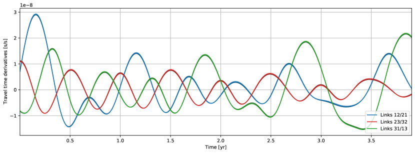
Figure 2: Light travel time derivatives for realistic orbits.

The inter-spacecraft interferometer mixes the local and distant beams. The beatnote phase $\Phi^{\text{isc}}_{ij}$ can easily be expressed as the difference of the beam phases,

$$\Phi^{\text{isc}}_{ij}=\Phi_{i\leftarrow j}-\Phi_{i}={\mathbf{D}_{ij}}\Phi_{j}-\Phi_{i}-({\mathbf{D}_{ij}}\nu_{j})H_{ij}\,\text{.}$$ (9)

In units of frequency, we have

$$\begin{split}&\nu^{\text{isc}}_{ij}=(1-\dot{d}_{ij}){\mathbf{D}_{ij}}\nu_{j}-\nu_{i}-({\mathbf{D}_{ij}}\nu_{j})\dot{H}_{ij}\,\text{,}\end{split}$$ (10)

where the term $\dot{d}_{ij}{\mathbf{D}_{ij}}\nu_{j}$ is the Doppler shift.

In eq. 10, the main in-band contribution is laser noise, which does not cancel out and remains orders of magnitude above the gravitational-wave signal $({\mathbf{D}_{ij}}\nu_{j})\dot{H}_{ij}\approx${10}^{-7}\text{\,}\mathrm{Hz}$$. In order to detect and extract gravitational information from the measurements, laser noise must be reduced by at least 8 orders of magnitude.

III Residual noise due to Doppler shifts in TDI

TDI is a technique proposed to reduce instrumental noises, including laser noise, to acceptable levels. The starting point for the main TDI algorithm is usually to compute the so-called intermediary variables $\xi$ and $\eta$, which are used to remove spacecraft jitter noise and reduce the number of lasers to three. While we already consider only one laser per spacecraft, we will further neglect spacecraft jitter noise, such that we can directly write $\eta_{ij}=\Phi^{\text{isc}}_{ij}$ in phase, or $\eta_{ij}=\nu^{\text{isc}}_{ij}$ in frequency.

The next step is to reduce laser noise. Several laser noise-reducing combinations have been proposed. E.g., the second-generation Michelson variable $X_{2}$ reads Tinto and Dhurandhar (2021)

$$\begin{split}&X_{2}=(1-{\mathbf{D}_{121}}-{\mathbf{D}_{12131}}+{\mathbf{D}_{1312121}})(\eta_{13}+{\mathbf{D}_{13}}\eta_{31})\\ &\quad-(1-{\mathbf{D}_{131}}-{\mathbf{D}_{13121}}+{\mathbf{D}_{1213131}})(\eta_{12}+{\mathbf{D}_{12}}\eta_{21})\,\text{.}\end{split}$$ (11)

The two other Michelson variables $Y_{2},Z_{2}$ are obtained by circular permutation of the indices $1\rightarrow 2\rightarrow 3\rightarrow 1$.

In the following, we shall ignore any technical reasons for imperfect laser noise reduction, such as flexing-filtering coupling Bayle et al. (2019), interpolation errors or ranging errors, and only consider the maximum theoretical laser noise reduction achievable.

In case of phase, we know that the residual laser noise in this variable is given by the non-commutation of delay operators Bayle et al. (2019),

$$X^{\Phi}_{2}=\commutator{\commutator{{\mathbf{D}_{131}}}{{\mathbf{D}_{121}}}}{{\mathbf{D}_{12131}}}\Phi_{1}\,\text{.}$$ (12)

Expanding this expression to second order in the average TT derivatives $\dot{d}$’s and first order in average TT second derivatives $\ddot{d}$’s, and assuming that these quantities are symmetric in $i$, $j$, the difference of the delays applied to the phase $\Phi_{1}$ in the two terms from eq. 12 reads

$$\Delta d=8\bar{d}\quantity(\bar{\dot{d}}_{12}^{2}-\bar{\dot{d}}_{31}^{2})-16\bar{d}^{2}\quantity(\bar{\ddot{d}}_{12}-\bar{\ddot{d}}_{31})\,\text{,}$$ (13)

where the first term matches the results of Bayle et al. (2019). In terms of power spectral density (PSD), we have

$$\opbraces{S_{X^{\Phi}_{2}}}(\omega)=\omega^{2}\Delta d^{2}\opbraces{S_{\Phi}}(\omega)\,\text{,}$$ (14)

where $\opbraces{S_{\Phi}}(\omega)$ is dominated by the PSD of the laser noise expressed in cycles.

Now, let us assess the impact of Doppler shifts if one uses naively the traditional second generation TDI algorithm using measurements in units of frequency. For this, we can insert eq. 10 in eq. 11. The only structural difference between eq. 10 and eq. 9 is the additional Doppler term $\dot{d}_{ij}{\mathbf{D}_{ij}}\nu_{j}$. Because TDI is a linear operation, we can immediately give the residual laser noise in terms of frequency when applying the same algorithm,

$$X^{\nu}_{2}=\commutator{\commutator{{\mathbf{D}_{131}}}{{\mathbf{D}_{121}}}}{{\mathbf{D}_{12131}}}\nu_{1}+\delta X^{\nu}_{2}\,\text{,}$$ (15)

where $\delta X^{\nu}_{2}$ is a function of the Doppler shifts,

$$\begin{split}\delta X^{\nu}_{2}&=(1-{\mathbf{D}_{131}}-{\mathbf{D}_{13121}}+{\mathbf{D}_{1213131}})\\ &\qquad\qquad\qquad\times(\dot{d}_{12}{\mathbf{D}_{12}}\nu_{2}+\dot{d}_{21}{\mathbf{D}_{121}}\nu_{1})\\ &\quad-(1-{\mathbf{D}_{121}}-{\mathbf{D}_{12131}}+{\mathbf{D}_{1312121}})\\ &\qquad\qquad\qquad\times(\dot{d}_{13}{\mathbf{D}_{13}}\nu_{3}+\dot{d}_{31}{\mathbf{D}_{131}}\nu_{1})\,\text{.}\end{split}$$ (16)

A rough estimation of this Doppler coupling can be computed from $\delta X^{\nu}_{2}\approx\bar{\dot{d}}\nu$. Plugging orders of magnitudes for the TTs derivatives and laser noise yields a Doppler coupling at ${10}^{-6}\text{\,}\mathrm{Hz}$, above the expected level for our GW signals (${10}^{-7}\text{\,}\mathrm{Hz}$). It is also above the level of the traditional residuals of TDI, given by the first term of eq. 15 and shown in fig. 3. As a consequence, the PSD of the residual noise for the $X_{2}^{\nu}$ TDI variable is dominated by the Doppler coupling,

$$\opbraces{S_{X^{\nu}_{2}}}(\omega)\approx\opbraces{S_{\delta X^{\nu}_{2}}}(\omega)\,\text{.}$$ (17)

Assuming that all laser frequencies are uncorrelated, a more precise computation yields the PSD of this extra residual noise,

$$\begin{split}\opbraces{S_{\delta X^{\nu}_{2}}}(\omega)&\approx 16\opbraces{S_{\nu}}\sin[2](\omega\bar{d})\sin[2](2\omega\bar{d})\\ &\qquad\times\quantity(\bar{\dot{d}}_{12}^{2}+\bar{\dot{d}}_{31}^{2}+(\bar{\dot{d}}_{12}-\bar{\dot{d}}_{31})^{2})\,\text{.}\end{split}$$ (18)

This is to be compared with the residual laser noise in terms of frequency when one disregards Doppler effects. It is given by replacing $\opbraces{S_{\Phi}}$ with $\opbraces{S_{\nu}}$ in eq. 14,

$$\opbraces{S_{[X^{\nu}_{2}]}}(\omega)=\omega^{2}\Delta d^{2}\opbraces{S_{\nu}}(\omega)\,\text{.}$$ (19)

In fig. 3, we show those analytical curves alongside the usual LISA Performance Model’s $1\text{\,}\mathrm{pm}$-noise allocation curve, given by

$$\begin{split}&\opbraces{S_{X_{2}^{\text{alloc}}}}(\omega)=64\omega^{2}\sin[2](\omega\bar{d})\sin[2](2\omega\bar{d})\\ &\qquad\times\quantity(\frac{$1\text{\,}\mathrm{p}\mathrm{m}\mathrm{Hz}^{-1/2}$}{\lambda})^{2}\quantity[1+\quantity(\frac{$2\text{\times}{10}^{-3}\text{\,}\mathrm{Hz}$}{\omega/2\pi})^{4}]\,\text{.}\end{split}$$ (20)

The extra residual laser noise due to Doppler terms is above or at the same level as the GW signal, and far above the usual laser noise residual when one disregards the Doppler effect. Therefore, a procedure to mitigate this effect is required if one wishes to use frequency measurements.

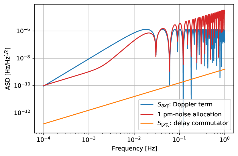
Figure 3: Amplitude spectral density of the second generation TDI combination when using measurements expressed in units of frequency. The blue curve shows the amplitude of Doppler-related terms, c.f. eq. 18, the orange curve shows the amplitude of the delay commutators, c.f. eq. 19, while the red curve presents the usual LISA $1\text{\,}\mathrm{pm}$-noise allocation, c.f. eq. 20. The light travel times used in this simulation are presented in fig. 2.

IV Adapting time-delay interferometry for Doppler shifts

As mentioned in the previous section, accounting for the Doppler effect in the inter-spacecraft beatnote frequency comes down to replacing the delay operator ${\mathbf{D}_{ij}}$ in eq. 9 by $(1-\dot{d}_{ij}){\mathbf{D}_{ij}}$. We can formalize it by introducing the Doppler-delay operator,

$${\dot{\mathbf{D}}_{ij}}=(1-\dot{d}_{ij}){\mathbf{D}_{ij}}\,\text{,}$$ (21)

such that laser noise entering eq. 10 takes the same algebraic form as its phase counterpart eq. 9,

$$\nu^{\text{isc}}_{ij}={\dot{\mathbf{D}}_{ij}}\nu_{j}-\nu_{i}+({\mathbf{D}_{ij}}\nu_{j})\dot{H}_{ij}\,\text{.}$$ (22)

We now introduce a new type of second generation TDI combination by considering the standard expression from eq. 11 but using the Doppler-delay operators introduced in eq. 21. The new TDI variable writes

$$\begin{split}&\dot{X}_{2}=(1-{\dot{\mathbf{D}}_{121}}-{\dot{\mathbf{D}}_{12131}}+{\dot{\mathbf{D}}_{1312121}})(\eta_{13}+{\dot{\mathbf{D}}_{13}}\eta_{31})\\ &\quad-(1-{\dot{\mathbf{D}}_{131}}-{\dot{\mathbf{D}}_{13121}}+{\dot{\mathbf{D}}_{1213131}})(\eta_{12}+{\dot{\mathbf{D}}_{12}}\eta_{21})\,\text{.}\end{split}$$ (23)

The algebraic form of this expression is now identical in phase and frequency, and we immediately recover the residual noise given in eq. 14,

$$\dot{X}^{\nu}_{2}=\commutator{\commutator{{\dot{\mathbf{D}}_{131}}}{{\dot{\mathbf{D}}_{121}}}}{{\dot{\mathbf{D}}_{12131}}}\nu_{1}\,\text{.}$$ (24)

A direct comparison with eq. 15 demonstrates that the new TDI variable introduced in eq. 23 is not impacted by the Doppler noise $\delta X_{2}^{\nu}$.

To compute the PSD of the $\dot{X}_{2}^{\nu}$ residual laser noise, we study the commutator of Doppler-delay operators

$$y=\commutator{{\dot{\mathbf{D}}_{i_{1}j_{1}}}\dots\dot{\mathbf{D}}_{i_{n}j_{n}}}{{\dot{\mathbf{D}}_{k_{1}l_{1}}}\dots\dot{\mathbf{D}}_{k_{n}l_{n}}}\,\text{.}$$ (25)

As one can observe in fig. 2, the light TT derivatives evolve slowly with time, with $\ddot{d}\Delta t\sim 10^{-14}\ll\dot{d}\sim 10^{-8}$ if $\Delta t\sim$10\text{\,}\mathrm{s}$$ is the timescale of the TTs considered here. Therefore, we can assume that $\dot{d}$’s are constant when computing $y$. Equation 25 can then be factored as

$$\begin{split}y=\quantity(\prod_{m=1}^{n}{(1-\dot{d}_{i_{m}j_{m}})})\quantity(\prod_{m=1}^{n}{(1-\dot{d}_{k_{m}l_{m}})})\times\\ \commutator{{\mathbf{D}_{i_{1}j_{1}}}\dots\mathbf{D}_{i_{n}j_{n}}}{{\mathbf{D}_{k_{1}l_{1}}}\dots\mathbf{D}_{k_{n}l_{n}}}\,\text{.}\end{split}$$ (26)

The factor that contains the TT derivatives is a constant, which, to first order, deviates from 1 by $2\bar{\dot{d}}n\approx${10}^{-7}$$. We can therefore neglect it when estimating the PSD. For this reason, the PSD of the laser noise residual for the new TDI variable introduced in eq. 23 is then given by

$$\opbraces{S_{\dot{X}^{\nu}_{2}}}(\omega)=\opbraces{S_{[X^{\nu}_{2}]}}(\omega)\,,$$ (27)

whose expression is explicitly given in eq. 19. A direct comparison with eq. 17 shows that the PSD of the new ${\dot{X}}_{2}^{\nu}$ TDI variable is not impacted by the unacceptably large contribution from $\delta X_{2}^{\nu}$.

The method presented in this section which consists in replacing ${\mathbf{D}_{ij}}$ by ${\dot{\mathbf{D}}_{ij}}$ in the usual TDI combinations in order to remove the effect of Doppler shift is very general and can be applied to any TDI combination.

V Simulation results

Using LISANode Bayle (2019) and lisainstrument, a Python simulator based on LISANode, we simulated the interferometric measurements as frequency deviations from the average beatnote frequencies. These frequency deviations include only laser noise, which is Doppler-shifted during propagation. We assumed 3 free-running lasers for this study, and used a high sampling rate, such that effects of onboard filtering appear off band. We used the same realistic orbits and light travel times as presented in fig. 2, and simulated ${10}^{7}$ samples, i.e., a bit less than $12$ days.

The TDI processing was performed using PyTDI. In fig. 4, we compare 2 different scenarios using the same input data. The blue curve shows the amplitude spectral density (ASD) of the residual laser noise when the standard second-generation Michelson $X^{\nu}_{2}$ variable is used. We superimpose the model for the expected excess of noise $\delta X^{\nu}_{2}$ due to Doppler effect given in eq. 18, and check that it matches our simulated results. Alternatively, the orange curve shows the ASD of the residual laser noise when the Doppler-corrected second-generation Michelson $\dot{X}^{\nu}_{2}$ variable is used. It is superimposed with the analytical expectation given in eq. 27 in most of the band, until we reach a noise floor around $2\text{\times}{10}^{-12}\text{\,}\mathrm{Hz}\mathrm{/}\sqrt{\mathrm{Hz}}$. This noise floor is in agreement with the numerical accuracy typically achieved in our simulations.

These simulations confirm the analytical results developed in the previous section. In particular, it shows that the residual noise of the new TDI variable introduced in eq. 23 is similar to the one obtained with the standard TDI combinations when the Doppler effect is neglected. Say in other words, the TDI variable corrects efficiently for the Doppler contribution which otherwise induces an unacceptably large noise.

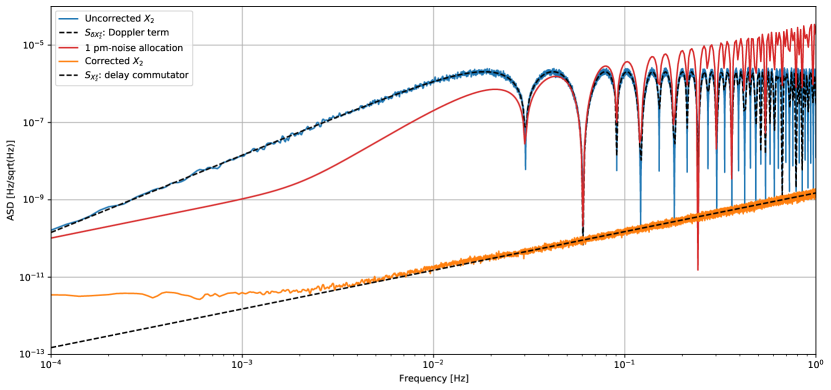
Figure 4: Amplitude spectral density of the residual laser noise in $X_{2}^{\nu}$ obtained using data in units of frequency, with the traditional algorithms (in blue) and Doppler correction (in orange). The theoretical models from Eqs. (18) and (19) are superimposed as black dashed lines. These curves need to be compared with the $1\text{\,}\mathrm{pm}$-noise allocation (in red).

VI Conclusion

In this paper, we show that the TDI combinations found in the literature Tinto and Dhurandhar (2021) do not reduce laser noise to required levels when applied to data in units of frequency and we provide an analytical formulation of the additional residual noise. We then propose a technique to adapt existing TDI combinations to data in units of frequency. We show through analytical studies, as well as with numerical simulations that we recover the original laser-noise reduction performance, compatible with requirements to detect and exploit GWs signals.

TDI is required to suppress primary noises in the interferometric measurements to levels below that of GW signals. Existing formulations are based on the assumption that these measurements are expressed in terms of phase, or disregard the impact of Doppler shifts when data in frequency are used Tinto and Dhurandhar (2021). However, applying these TDI algorithms to data in units of frequency yields extra noise residuals due to the Doppler shift induced by the time variation of the arm lengths. This extra noise residuals are larger than GW signals. To account for Doppler shifts we reformulate the TDI combinations by replacing delay operators by their Doppler equivalent, which not only shift measurement in time but also scale them by the corresponding Doppler factor, see eq. 21. We show that this general procedure yields new TDI combinations, whose performance when applied to measurements in frequency match that of the traditional combinations when working in units of phase.

This is a major result to study the impact of different physical units in LISA data processing. We show that laser noise reduction can reach similar levels using phase or frequency measurements. Nevertheless, computing the TDI using frequency measurements require the knowledge of both the TT and their time derivatives while only the TT are needed in order to construct TDI variables using phase measurements. This might impact the development of a Kalman filter whose goal is to provide an estimate of the TT Wang et al. (2014, 2015). Finally, it is known that the clocks from the various spacecraft will drift with respect to each other because of relativistic effects Pireaux (2007) and because of clock noise. Therefore, the LISA pre-processing will also include a synchronization of the clocks from the 3 spacecraft Tinto and Dhurandhar (2021). How this synchronization will impact the construction of TDI variables is currently under exploration and might differ if one uses phase or frequency units. A detailed study of the interplay of TDI with clock synchronization is left for a dedicated study. Finally, let us mention that using frequency units to perform the data analysis of LISA may also impact the sources parameters inference since the TDI response function used in Bayesian algorithm may have to include the currently neglected Doppler correction.

Appendix A Mapping between conventions

The following table gives the mapping between the double-index conventions used in the article, and historic ones using primed indices, used in, e.g., Bayle et al. (2019); Bayle (2019); Otto (2015); Petiteau et al. (2008). We give the correspondence for optical bench and associated subsystems and quantities, and that for light TTs and their derivatives.

Double-index	Primed indices for optical benches	Primed indices for light TTs
12 (e.g., $\nu^{\text{isc}}_{12}$ or $d_{12}$)	1 (e.g., $\nu^{\text{isc}}_{1}$)	3 (e.g., $d_{3}$)
23 (e.g., $\nu^{\text{isc}}_{23}$ or $d_{23}$)	2 (e.g., $\nu^{\text{isc}}_{2}$)	1 (e.g., $d_{1}$)
31 (e.g., $\nu^{\text{isc}}_{31}$ or $d_{31}$)	3 (e.g., $\nu^{\text{isc}}_{3}$)	2 (e.g., $d_{2}$)
13 (e.g., $\nu^{\text{isc}}_{13}$ or $d_{13}$)	$1^{\prime}$ (e.g., $\nu^{\text{isc}}_{1^{\prime}}$)	$2^{\prime}$ (e.g., $d_{2^{\prime}}$)
32 (e.g., $\nu^{\text{isc}}_{32}$ or $d_{32}$)	$3^{\prime}$ (e.g., $\nu^{\text{isc}}_{3^{\prime}}$)	$1^{\prime}$ (e.g.,  $d_{1^{\prime}}$)
21 (e.g., $\nu^{\text{isc}}_{21}$ or $d_{21}$)	$2^{\prime}$ (e.g., $\nu^{\text{isc}}_{2^{\prime}}$)	$3^{\prime}$ (e.g.,  $d_{3^{\prime}}$)

References

- Abbott et al. (2016) B. P. Abbott et al. (LIGO Scientific Collaboration and Virgo Collaboration), Phys. Rev. Lett. 116, 061102 (2016).
- Abbott et al. (2019) B. P. Abbott et al. (LIGO Scientific, Virgo), Phys. Rev. X 9, 031040 (2019), arXiv:1811.12907 [astro-ph.HE] .
- Amaro-Seoane et al. (2017) P. Amaro-Seoane et al. (LISA Collaboration), Laser Interferometer Space Antenna, Tech. Rep. (LISA Consortium, 2017) arXiv.org:1702.00786 [astro-ph] .
- Giampieri et al. (1996) G. Giampieri, R. W. Hellings, M. Tinto, and J. E. Faller, Optics Communications 123, 669 (1996).
- Armstrong et al. (1999) J. W. Armstrong, F. B. Estabrook, and M. Tinto, The Astrophysical Journal 527, 814 (1999).
- Tinto and Armstrong (1999) M. Tinto and J. W. Armstrong, Phys. Rev. D 59, 102003 (1999).
- Tinto and Dhurandhar (2021) M. Tinto and S. V. Dhurandhar, Living Reviews in Relativity 24, 1 (2021).
- Tinto et al. (2002) M. Tinto, F. B. Estabrook, and J. W. Armstrong, Phys. Rev. D 65, 082003 (2002).
- Shaddock et al. (2003) D. A. Shaddock, M. Tinto, F. B. Estabrook, and J. W. Armstrong, Phys. Rev. D 68, 061303 (2003), gr-qc/0307080 .
- Cornish and Hellings (2003) N. J. Cornish and R. W. Hellings, Classical and Quantum Gravity 20, 4851 (2003), gr-qc/0306096 .
- Tinto et al. (2004) M. Tinto, F. B. Estabrook, and J. W. Armstrong, Phys. Rev. D 69, 082001 (2004), gr-qc/0310017 .
- Schwarze et al. (2019) T. S. Schwarze, G. Fernández Barranco, D. Penkert, M. Kaufer, O. Gerberding, and G. Heinzel, Phys. Rev. Lett. 122, 081104 (2019), arXiv:1810.00728 [astro-ph.IM] .
- Otto (2015) M. Otto, Time-Delay Interferometry Simulations for the Laser Interferometer Space Antenna, Ph.D. thesis, Leibniz U., Hannover (2015).
- Laporte et al. (2017) M. Laporte, H. Halloin, E. Bréelle, C. Buy, P. Grüning, and P. Prat, J. Phys. Conf. Ser. 840, 012014 (2017).
- Cruz et al. (2006) R. J. Cruz, J. I. Thorpe, M. Hartman, and G. Mueller, Proceedings, 6th International LISA Symposium on Laser interferometer space antenna: Greenbelt, USA, June 19-23, 2006, AIP Conf. Proc. 873, 319 (2006).
- Vallisneri (2005) M. Vallisneri, Phys. Rev. D 71, 022001 (2005), arXiv:gr-qc/0407102 .
- Petiteau et al. (2008) A. Petiteau, G. Auger, H. Halloin, O. Jeannin, E. Plagnol, S. Pireaux, T. Regimbau, and J.-Y. Vinet, Phys. Rev. D 77, 023002 (2008), arXiv:0802.2023 [gr-qc] .
- Bayle et al. (2019) J.-B. Bayle, M. Lilley, A. Petiteau, and H. Halloin, Phys. Rev. D 99, 084023 (2019), arXiv:1811.01575 [astro-ph.IM] .
- Dhurandhar et al. (2005) S. V. Dhurandhar, K. Rajesh Nayak, S. Koshti, and J. Y. Vinet, Class. Quant. Grav. 22, 481 (2005), arXiv:gr-qc/0410093 .
- Nayak et al. (2006) K. R. Nayak, S. Koshti, S. V. Dhurandhar, and J. Y. Vinet, Class. Quant. Grav. 23, 1763 (2006).
- Joffre et al. (2020) E. Joffre, D. Wealthy, I. Fernandez, C. Trenkel, P. Voigt, T. Ziegler, and W. Martens, Advances in Space Research (2020), https://doi.org/10.1016/j.asr.2020.09.034.
- Martens and Joffre (2021) W. Martens and E. Joffre, (2021), arXiv:2101.03040 [gr-qc] .
- Heinzel et al. (2011) G. Heinzel, J. José Esteban, S. Barke, M. Otto, Y. Wang, A. F. Garcia, and K. Danzmann, Classical and Quantum Gravity 28, 094008 (2011).
- José Esteban et al. (2011) J. José Esteban, A. F. García, S. Barke, A. M. Peinado, F. Guzmán Cervantes, I. Bykov, G. Heinzel, and K. Danzmann, Optics Express 19, 15937 (2011).
- Wang et al. (2014) Y. Wang, G. Heinzel, and K. Danzmann, Phys. Rev. D 90, 064016 (2014), arXiv:1402.6222 [gr-qc] .
- Wang et al. (2015) Y. Wang, G. Heinzel, and K. Danzmann, Phys. Rev. D 92, 044037 (2015), arXiv:1503.08377 [gr-qc] .
- Bayle (2019) J.-B. Bayle, Simulation and Data Analysis for LISA, Ph.D. thesis, Université de Paris (2019).
- Pireaux (2007) S. Pireaux, Classical and Quantum Gravity 24, 2271 (2007), arXiv:gr-qc/0703119 .