Internally Hankel $k$-positive systems

Abstract

The classes of externally Hankel $k$-positive LTI systems and autonomous $k$-positive systems have recently been defined, and their properties and applications began to be explored using the framework of total positivity and variation diminishing operators. In this work, these two system classes are subsumed under a new class of internally Hankel $k$-positive systems, which we define as state-space LTI systems with $k$-positive controllability and observability operators. We show that internal Hankel $k$-positivity is a natural extension of the celebrated property of internal positivity ($k=1$), and we derive tractable conditions for verifying the cases $k>1$ in the form of internal positivity of the first $k$ compound systems. As these conditions define a new positive realization problem, we also discuss geometric conditions for when a minimal internally Hankel $k$-positive realization exists. Finally, we use our results to establish a new framework for bounding the number of over- and undershoots in the step response of general LTI systems.

1 Introduction

Externally positive linear time-invariant (LTI) systems

$$x(t+1) =Ax(t)+bu(t)$$ (1)

$$y(t) =cx(t),$$

mapping nonnegative inputs $u(t)$ to nonnegative outputs $y(t)$ have been recognized as an important system class at least since the exposition by Luenberger [24], but many of their favourable properties have only recently been exploited [31, 34, 10, 32]. Particular emphasis has been given to the subclass of internally positive systems, that is, externally positive systems such that $x(t)$ remains in the nonnegative orthant for nonnegative $u(t)$. As such systems are characterized by nonnegative system matrices $A$, $b$ and $c$, they can be studied with finite-dimensional nonnegative matrix analysis [6], an advantage that motivated the search for conditions under which an externally positive system admits an internally positive realization [28, 2, 4].

At the same time, externally positive systems have been studied for over a century from the viewpoint of fields such as statistics and interpolation theory, leading to the theory of total positivity [20]. Central to this theory is the study of variation-diminishing convolution operators

$$y(t)=\sum_{\tau=-\infty}^{\infty}g(t-\tau)u(\tau),$$ (2)

with nonnegative kernels $g$, that bound the variation (number of sign changes) of $y(t)$ by the variation of $u(t)$. More generally, a linear mapping $u\mapsto Gu$ is called $k$-variation diminishing ($\text{VD}_{k}$) if it maps an input $u$ with at most $k$ sign changes to an output $Gu$ whose number of sign changes do not exceed those of $u$; if the order in which sign changes occur is preserved whenever $u$ and $Gu$ share the same number of sign variations, the $\text{VD}_{k}$ property is said to be order-preserving ($\text{OVD}_{k}$). A core result of total positivity is an algebraic characterization: an operator is $\text{OVD}_{k}$ if and only its matrix representation is ${k\text{-positive}}$, that is, all the minors of order up to $k$ in that matrix are nonnegative [17, 20]; total positivity refers to the case when this is true for all $k$. Under this framework, externally positive LTI systems are associated with $\text{OVD}_{0}$ Hankel and Toeplitz operators, while for internally positive systems $x\mapsto Ax$ as well as the controllablity and observability operators are $\text{OVD}_{0}$.

Despite the link between positive systems and variation-diminishing operators, it was not until very recently that $\text{OVD}_{k-1}$ and $k$-positivity have been studied as properties of LTI systems when $k>1$. New results, with applications in non-linear systems analysis and model order reduction, have so far focused on two distinct cases: the external case [16, 17, 15], where $\text{OVD}_{k}$ is considered as a property of system convolution operators; and related autonomous cases [26, 1], which concern $k$-positivity of the state-space matrix $A$ with $b=0$. A main result of [17] characterizes (externally) Hankel $k$-positive systems, i.e., systems with $\text{OVD}_{k-1}$ Hankel operators, in terms of the external positivity of all so-called $j$-compound systems, $1\leq j\leq k$, whose impulse responses are given by consecutive $j$-minors of the Hankel operator’s matrix representation.

In this paper, we develop a realization theory of Hankel $k$-positivity based on the notion of internally Hankel $k$-positive systems, which we define as state-space systems where the controllability and observability operators as well as $A$ are $\text{OVD}_{k-1}$. Not only does this theory enable the study of variation-diminishing systems through finite-dimensional analysis, but it also establishes an important first bridge between the aforementioned autonomous and external notions. Our main result is a finite-dimensional, tractable condition for the verification of the $\text{OVD}_{k-1}$ property of the controllability and observability operators. Using this result, internal Hankel $k$-positivity can be completely characterized in terms of the existence of a realization that renders all $j$-compound systems internally positive, $1\leq j\leq k$. We then use these insights to discuss geometric conditions for the existence of minimal internally Hankel ${k\text{-positive}}$ realizations, as previously done for the special case $k=1$ in [28]. In particular, it is easy to verify then that all relaxation systems [35] ($k=\infty$) have a minimal internally Hankel totally positive realization.

As a practical application, we show how our results can be used to obtain upper bounds on the number of over- and undershoots in the step response of an LTI system. This is a classical control problem that lies at the heart of the rise-time-settling-time trade-off [3], and for which several lower bounds [7, 33, 23, 22], but few upper bounds [23, 22] have been found. Our approach can be seen as a direct generalization of [23, 22]. Non-linear extensions of this problem are of interest both in control [21] and online learning, in the form of (static) regret [29]; we thus envision our work as the basis for possible interdisciplinary applications. Other possible contributions resulting from non-linear extension are discussed in [17].

The paper is organized as follows. In the preliminaries, we recap total positivity theory and externally Hankel $k$-positive systems. Then, we introduce the concept of internal Hankel $k$-positivity and present our main results on its characterization. Subsequently, extensions to continuous-time and applications to the determination of impulse response zero-crossings are discussed. We conclude with illustrative examples and a summary of open problems.

2 Preliminaries

This work lies at the interface between positive control systems and total positivity theory. Alongside some standard notation, this section briefly introduces key concepts and results from these fields, including recent results on externally $k$-positive LTI systems, which are crucial to the motivation of our main results.

2.1 Notations

We write $\mathds{Z}$ for the set of integers and $\mathds{R}$ for the set of reals, with $\mathds{Z}_{\geq 0}$ and $\mathds{R}_{\geq 0}$ standing for the respective subsets of nonnegative elements; the corresponding notation with strict inequality is also used for positive elements. The set of real sequences with indices in $\mathds{Z}$ is denoted by $\mathds{R}^{\mathds{Z}}$. For matrices $X=(x_{ij})\in\mathds{R}^{n\times m}$, we say that $X$ is nonnegative, $X\geq 0$ or $X\in\mathds{R}^{n\times m}_{\geq 0}$ if all elements $x_{ij}\in\mathds{R}_{\geq 0}$ ; again, we use the corresponding notations in case of positivity. The notations also apply to sequences $x=(x_{i})\in\mathds{R}^{\mathds{Z}}$. Submatrices of $X\in\mathds{R}^{n\times m}$ are denoted by $X_{I,J}:=(x_{ij})_{i\in I,j\in J}$, where $I{\subseteq}\{1,\dots,n\}$ and $J{\subseteq}\{1,\dots,m\}$. If $I$ and $J$ have cardinality $r$, then $\det(X_{I,J})$ is referred to as an $r$-minor, and as a consecutive $r$-minor if $I$ and $J$ are intervals. For $X\in\mathds{R}^{n\times n}$, $\sigma(X)=\{\lambda_{1}(X),\dots,\lambda_{n}(X)\}$ denotes the spectrum of $X$, where the eigenvalues are ordered by descending absolute value, i.e., $\lambda_{1}(X)$ is the eigenvalue with the largest magnitude, counting multiplicity. In case that the magnitude of two eigenvalues coincides, we sub-sort them by decreasing real part. If there exists a permutation matrix $P=[P_{1},P_{2}]$ so that $P_{2}^{T}XP_{1}=0$, then $X$ is called reducible and otherwise irreducible. Further, $X$ is said to be positive semidefinite, $X\succeq 0$, if $X=X^{\mathsf{T}}$ and $\sigma(X)\subset\mathds{R}_{\geq 0}$. Further, we use $I_{n}$ to denote the identity matrix in $\mathds{R}^{n\times n}$. For $\mathcal{S}\subset\mathds{R}^{n}$, we denote its closure, convex hull and convex conic hull by $\textnormal{cl}(\mathcal{S})$, $\textnormal{conv}(\mathcal{S})$ and $\textnormal{cone}(\mathcal{S})$, respectively. $\mathcal{S}$ is a polyhedral cone, if there exists $k\in\mathds{Z}_{>0}$ and $P\in\mathds{R}^{n\times k}$ such that $\mathcal{S}=\{Px:x\in\mathds{R}^{k}_{\geq 0}\}=:\textnormal{cone}(P)$. For $A\in\mathds{R}^{n\times n}$, $\mathcal{S}$ is said to be $A$-invariant, $A\mathcal{S}\subset\mathcal{S}$, if $Ax\in\mathcal{S}$ for all $x\in\mathcal{S}$. For a subset $\mathcal{S}\subset\mathds{Z}$, we write $g\geq 0$ or $g\in\mathds{R}^{\mathcal{S}}_{\geq 0}$ if $g:\mathcal{S}\to\mathds{R}_{\geq 0}$ is a nonnegative function (sequence) and

$$\mathds{1}_{\mathcal{S}}(t):=\begin{cases}1&t\in\mathcal{S}\\ 0&t\notin\mathcal{S}\end{cases}$$

for the (1-0) indicator function. In particular, we denote the Heaviside function by $s(t):=\mathds{1}_{\mathds{R}_{\geq 0}}(t)$ and the unit pulse function by $\delta(t)$. The set of all absolutely summable sequences is denoted by $\ell_{1}$ and the set of bounded sequences by $\ell_{\infty}$.

2.2 Linear discrete-time systems

We consider discrete-time, linear time-invariant (LTI) systems with input $u$ and output $y$. The output $g(t)=y(t)$ corresponding to $u(t)=\delta(t)$ is called the impulse response. Throughout this work, we assume that $g\in\ell_{1}$ and $u\in\ell_{\infty}$. The transfer function of the system is given by

$$G(z)=\sum_{t=0}^{\infty}g(t)z^{-t}=\frac{r\prod_{i=1}^{m}(z-z_{i})}{\prod_{j=1}^{n}(z-p_{i})}$$ (3)

where $r\in\mathds{R}$, and $p_{i}$ and $z_{i}$ are referred to as poles and zeros, both of which are sorted in same way as the eigenvalues of a matrix. Without loss of generality, we assume that $g(0)=0$ ($m<n$). The tuple $(A,b,c)$ is referred to as a state-space realization of $G(z)$ if eq. 1 holds, with stable $A\in\mathds{R}^{n\times n}$, and $b,c^{\mathsf{T}}\in\mathds{R}^{n}$. It holds then that

$$g(t)=cA^{t-1}b\,s(t-1).$$

We assume that the set of poles and the set of zeros of a transfer function are disjoint, and define the order of a system as the number of poles of $G(z)$. A realization $(A,b,c)$ is called minimal if the eigenvalues of $A$ are precisely the poles of $G(z)$. For $t\geq 0$, the Hankel operator

$$(\mathcal{H}_{g}u)(t) :=\sum_{\tau=-\infty}^{-1}g(t-\tau)u(\tau)=\sum_{\tau=1}^{\infty}g(t+\tau)u(-\tau)$$ (4)

describes the evolution of $y$ after $u$ has been turned off at $t=0$, i.e., $u(t)=u(t)(1-s(t))$. It obeys the factorization

$$\mathcal{H}_{g}u=\mathcal{O}(A,c)(\mathcal{C}(A,b)u)$$ (5)

with the controllability and observability operators given by

$$x(0)={\mathcal{C}}(A,b)u :=\sum_{t=-\infty}^{-1}A^{-t-1}bu(t),\ u\in\ell_{\infty}$$ (6a)

$$({\mathcal{O}}(A,c)x_{0})(t) :=cA^{t}x_{0},\ x_{0}\in\mathds{R}^{n},\ t\in\mathds{Z}_{\geq 0}$$ (6b)

Finally, for $t,j\in\mathds{Z}_{>0}$, we will often make use of the Hankel matrix

$$H_{g}(t,j) :=\begin{pmatrix}g(t)&g(t+1)&\dots&g(t+j-1)\\ g(t+1)&g(t+2)&\dots&g(t+j)\\ \vdots&\vdots&\ddots&\vdots\\ g(t+j-1)&g(t+j)&\dots&g(t-2(j-1))\\ \end{pmatrix}={\mathcal{O}^{j}}(A,c)A^{t-1}{\mathcal{C}^{j}}(A,b)$$ (7a)

where

$${\mathcal{C}^{j}}(A,b) :=\begin{pmatrix}b&Ab&\dots&A^{j-1}b\end{pmatrix}$$ (7b)

$${\mathcal{O}^{j}}(A,c) :={\mathcal{C}^{j}}(A^{\mathsf{T}},c^{\mathsf{T}})^{\mathsf{T}}.$$ (7c)

2.3 Total positivity and the variation diminishing property

A central idea in this work is that positivity is an instance of the variation diminishing property. The variation of a sequence or vector $u$ is defined as the number of sign-changes in $u$, i.e.,

$$\text{S}(u):=\sum_{i\geq 1}\mathds{1}_{\mathds{R}_{<0}}(\tilde{u}_{i}\tilde{u}_{i+1}),\quad\text{S}(0):=0$$

where $\tilde{u}_{i}$ is the vector resulting form deleting all zeros in $u$.

Definition 2.1.

A linear map $u\mapsto Xu$ is said to be order-preserving ${k}$-variation diminishing ($\text{OVD}_{k}$), $k\in\mathds{Z}_{\geq 0}$, if for all $u$ with $\text{S}(u)\leq k$ it holds that

1. $\text{S}(Xu)\leq\text{S}(u)$.

2. The sign of the first non-zero elements in $u$ and $Xu$ coincide whenever $\text{S}(u)=\text{S}(Xu)$.

If the second item is dropped, then $u\mapsto Xu$ is called ${k}$-variation diminishing ($\text{VD}_{k}$). For brevity, we simply say $X$ is $\text{(O)}\text{VD}_{k}$.

The $\text{OVD}_{k}$ property extends the the cone-invariance of nonnegative matrices, namely $X\in\mathds{R}^{n\times m}_{\geq 0}$ is $\text{OVD}_{0}$, because $X\mathds{R}_{\geq 0}^{m}\subseteq\mathds{R}_{\geq 0}^{n}$. For generic $k$, total positivity theory provides algebraic conditions for the $\text{OVD}_{k}$ property by means of compound matrices. To define these, let the $i$-th elements of the $r$-tuples in

$$\mathcal{I}_{n,r}:=\{v=\{v_{1},\dots,v_{r}\}\subset\mathds{N}:1\leq v_{1}<v_{2}<\dots<v_{r}\leq n\}$$

be defined by lexicographic ordering. Then, the $(i,j)$-th entry of the r-th multiplicative compound matrix ${X}_{[r]}\in\mathds{R}^{\binom{n}{r}\times\binom{m}{r}}$ of $X\in\mathds{R}^{n\times m}$ is defined by $\det(X_{(I,J)})$, where $I$ is the $i$-th and $J$ is the $j$-th element in $\mathcal{I}_{n,r}$ and $\mathcal{I}_{m,r}$, respectively. For example, if $X\in\mathds{R}^{3\times 3}$, then ${X}_{[2]}$ reads

$$\begin{pmatrix}\det(X_{\{1,2\},\{1,2\}})&\det(X_{\{1,2\},\{1,3\}})&\det(X_{\{1,2\},\{2,3\}})\\ \det(X_{\{1,3\},\{1,2\}})&\det(X_{\{1,3\},\{1,3\}})&\det(X_{\{1,3\},\{2,3\}})\\ \det(X_{\{2,3\},\{1,2\}})&\det(X_{\{2,3\},\{1,3\}})&\det(X_{\{2,3\},\{2,3\}})\\ \end{pmatrix}.$$

Notice a nonnegative matrix verifies $X_{[1]}=X\geq 0$, which is equivalent to $X$ being $\text{OVD}_{0}$. This can be generalized through the compound matrix as follows [17, 20].

Definition 2.2.

Let $X\in\mathds{R}^{n\times m}$ and $k\leq\min\{m,n\}$. $X$ is called k-positive if ${X}_{[j]}\geq 0$ for $1\leq j\leq k$, and strictly k-positive if ${X}_{[j]}>0$ for $1\leq j\leq k$. In case $k=\min\{m,n\}$, $X$ is called (strictly) totally positive.

Proposition 2.1.

Let $X\in\mathds{R}^{n\times m}$ with $n\geq m$. Then, $X$ is ${k\text{-positive}}$ with $1\leq k\leq m$ if and only if $X$ is $\text{OVD}_{k-1}$.

The Cauchy-Binet formula implies the following important properties [13].

Lemma 2.1.

Let $X\in\mathds{R}^{n\times p}$ and $Y\in\mathds{R}^{p\times m}$.

1. ${(XY)}_{[r]}={X}_{[r]}{Y}_{[r]}$.

2. $\sigma({X}_{[r]})=\{\prod_{i\in I}\lambda_{i}(X):I\in\mathcal{I}_{n,r}\}$.

3. ${X^{\mathsf{T}}}_{[r]}=({X}_{[r]})^{\mathsf{T}}$.

In conjunction with the Perron-Frobenius theorem [30, 14], this yields a spectral characterization of ${k\text{-positive}}$ matrices as follows.

Corollary 2.1.

Let $X\in\mathds{R}^{n\times n}$ be k-positive such that ${X}_{[j]}$ is irreducible for $1\leq j\leq k$. Then,

1. $\lambda_{1}(X)>\dots>\lambda_{k}(X)>0$.

2. $\lambda_{1}({X}_{[j]})=\prod_{i=1}^{j}\lambda_{i}(X)>0$.

3. ${\begin{pmatrix}\xi_{1}&\dots&\xi_{j}\end{pmatrix}}_{[j]}\in\mathds{R}^{\binom{n}{j}}_{>0}$, $1\leq j\leq k$, where $\xi_{i}$ is the eigenvector associated with $\lambda_{i}(X)$ for $1\leq i\leq k$.

The next result shows that it often suffices to check consecutive minors to verify $k$-positivity vis-a-vis a combinatorial number of minors [20, 9].

Proposition 2.2.

Let $X\in\mathds{R}^{n\times m}$, $k\leq\min\{n,m\}$ be such that

1. all consecutive $r$-minors of $X$ are positive, $1\leq r\leq k-1$,

2. all consecutive $k$-minors of $X$ are nonnegative (positive).

Then, $X$ is (strictly) k-positive.

Finally, to be able to apply Proposition 2.2 to matrices lacking strictly positive intermediate $j$-minors, we will make use of the following.

Proposition 2.3.

Let $F(\sigma)\in\mathds{R}^{n\times n}$ be given by $F(\sigma)_{ij}=e^{-\sigma(i-j)^{2}}$, with $\sigma\geq 0$, and let $X\in\mathds{R}^{n\times m}$ with $m\leq n$. Then for $r\leq m$, the following hold:

1. $F(\sigma)$ is strictly totally positive.

2. $F(\sigma)\to I$ as $\sigma\to\infty$, and $F(\sigma)X\to X$ as $\sigma\to\infty$.

3. if ${X}_{[r]}\geq 0$, and if $\textnormal{rank}\,X=m$, then ${(F(\sigma)X)}_{[r]}>0$ for all $\sigma>0$.

4. if ${(F(\sigma)X)}_{[r]}\geq 0$ for all $\sigma>0$, then ${X}_{[r]}\geq 0$.

Proof.

Parts (i)-(iii) are proven in [20, p.220], while part (iv) is a consequence of (ii) and the continuity of the minors of a matrix in its entries (see e.g. [19]). ∎

2.4 Hankel $k$-positivity and compound systems

The $\text{OVD}_{k}$ property of LTI systems eq. 1 has been studied in [17], where a distinction is made between LTI systems with $\text{OVD}_{k}$ Toeplitz and Hankel operators. The latter are particularly relevant to this work.

Definition 2.3.

A system $G(z)$ is called Hankel ${k\text{-positive}}$ if $\mathcal{H}_{g}$ is $\text{OVD}_{k-1}$ ($k\geq 1$). If $k=\infty$, $G(z)$ is said to be Hankel totally positive.

In other words, $G(z)$ is $\text{OVD}_{k-1}$ from past inputs to future outputs. Note that if $G(z)$ is Hankel ${k\text{-positive}}$, then it is also Hankel ${j\text{-positive}}$, $1\leq j\leq k$. Since an $\text{OVD}_{k-1}$ $\mathcal{H}_{g}$ maps nonnegative inputs to nonnegative outputs, it can be verified that Hankel $1$-positivity coincides with the familiar property of external positivity.

Definition 2.4.

$G(z)$ is externally positive if $y\in\mathds{R}^{\mathds{Z}_{\geq 0}}_{\geq 0}$ for all $u\in\mathds{R}^{\mathds{Z}_{\geq 0}}_{\geq 0}$ (and $x(0)=0)$.

A central observation of [17] is the following characterization involving $k$-positive matrices.

Lemma 2.2.

A system $G(z)$ is Hankel $k$-positive if and only if for all $j\in\mathds{Z}_{>0}$, $H_{g}(1,j)$ is ${k\text{-positive}}$.

Using Propositions 2.2 and 2.3, it is easy to show that $k$-positivity of Hankel matrices only require checking the nonnegativity of consecutive minors [9]. From eq. 7a, each of these consecutive minors is given by

$$g_{[j]}(t):=\det(H_{g}(t,j)),$$

which is interpreted as the impulse response of an LTI system $G_{[j]}(z)$, called the $j$-th compound system. The compound systems feature in the following characterization.

Proposition 2.4.

Given $G(z)$ and $1\leq k\leq n$, the following are equivalent:

1. $G(z)$ is Hankel ${k\text{-positive}}$.

2. $G_{[j]}(z)$ is externally positive for $1\leq j\leq k$.

3. $H_{g}(1,k-1)\succ 0$, $H_{g}(2,k-1)\succeq 0$ and $G_{[k]}(z)$ is externally positive.

4. $G_{[j]}$ is Hankel ${k-j+1\text{-positive}}$ for $1\leq j\leq k$.

In particular, the equivalence between Hankel $\text{OVD}_{0}$ and external positivity becomes evident as both properties require $g_{[1]}=g\geq 0$ [10].

A key fact for our new investigations is that if $(A,b,c)$ is a realization of $G(z)$, then $G_{[j]}(z)$ can be realized as

$$({A}_{[j]},{{\mathcal{C}^{j}}(A,b)}_{[j]},{{\mathcal{O}^{j}}(A,c)}_{[j]}).$$ (8)

Note that by eq. 7a, $g_{[j]}=0$ if $j>n$, which is why $k=n$ coincides with the case $k=\infty$. The following pole constraints of Hankel ${k\text{-positive}}$ systems will also be important for our new developments.

Proposition 2.5.

Let $G(z)=\sum_{a=1}^{l}\sum_{b=1}^{m_{a}}\frac{r_{ba}}{(z-p_{a})^{b}}$ be Hankel ${k\text{-positive}}$. Then, $m_{1}=\dots=m_{k-1}=1$ and $p_{k-1}>0$ if $k\leq\sum_{a=1}^{l}m_{a}$. In particular, $G(z)$ is Hankel totally positive if and only if all poles are nonnegative and simple.

3 Internally Hankel $k$-positive systems

In this section, we introduce and study a subclass of Hankel ${k\text{-positive}}$ systems which admit state-space realizations such that the $\text{OVD}_{k-1}$ property also holds internally.

Definition 3.1.

$(A,b,c)$ is called internally Hankel ${k\text{-positive}}$ if $A$, ${\mathcal{C}}(A,b)$, and ${\mathcal{O}}(A,c)$ are $\text{OVD}_{k-1}$ ($k\geq 1$). If $k=\infty$, we say that $(A,b,c)$ is internally Hankel totally positive.

Internally Hankel ${k\text{-positive}}$ systems are, therefore, $\text{OVD}_{k-1}$ from past input $u$ to $x(0)$, and from $x(0)$ to all future $x(t)$ and future output $y$. In particular, by eq. 5, all internally Hankel ${k\text{-positive}}$ systems are also Hankel ${k\text{-positive}}$, and setting $u\equiv 0$ recovers the ${k\text{-positive}}$ property of autonomous systems as partially studied in [26, 1]. Thus, Definition 3.1 bridges the external and the autonomous notions of variation diminishing LTI systems. In the remainder of this section, we aim to answer the following main questions:

1. How does internal Hankel $k$-positivity manifest as tractable algebraic properties of $(A,b,c)$?

2. When does a system have a minimal internally Hankel $k$-positive realization?

Our answers will generalize the well-known case of $k=1$ [28, 2, 4, 10, 25], which, we will see, coincides with the familiar class of internally positive systems [10].

Definition 3.2.

$(A,b,c)$ is said to be internally positive if for all $u\in\mathds{R}^{\mathds{Z}_{\geq 0}}_{\geq 0}$ and all $x(0)\geq 0$, it follows that $y\in\mathds{R}^{\mathds{Z}_{\geq 0}}_{\geq 0}$ and $x(t)\geq 0$ for all $t\geq 0$.

In Section 4, our findings are extended to continuous-time systems, and we use our result to establish a framework that upper bounds the variation of the impulse response in arbitrary LTI systems.

3.1 Characterization of internally Hankel $k$-positive systems

We start by recalling the following well-known characterization of internal positivity in terms of system matrix properties [25].

Proposition 3.1.

$(A,b,c)$ is internally positive if and only if $A,b,c\geq 0$.

Therefore, internal positivity indeed implies that $(A,b,c)$ is internally Hankel $1$-positive (through Proposition 2.1). The converse can be seen from the following equivalences, which give a first characterization of internal Hankel $k$-positivity.

Lemma 3.1.

For $(A,b,c)$, the following are equivalent:

1. ${\mathcal{C}}(A,b)$ and ${\mathcal{O}}(A,c)$ are $\text{OVD}_{k-1}$, respectively.

2. For all $t\geq k$, ${\mathcal{C}^{t}}(A,b)$ and ${\mathcal{O}^{t}}(A,c)$ are ${k\text{-positive}}$, respectively.

In particular, $(A,b,c)$ is internally Hankel $k$-positive if and only if $A$, ${\mathcal{C}^{t}}(A,b)$ and ${\mathcal{O}^{t}}(A,b)$ are $k$-positive for all $t\geq k$.

Proof.

By Proposition 2.1, it suffices to show that ${\mathcal{C}}(A,b)$ is $\text{OVD}_{k-1}$ if and only if ${\mathcal{C}^{t}}(A,b)$ is $\text{OVD}_{k-1}$ for all $t\geq k$. For ${\mathcal{O}}(A,c)$, the proof is analogous via the duality eq. 7c.
$\Rightarrow$: Follows by considering inputs $u$ with $u(t)=0$ for $t\geq k$.
$\Leftarrow$: Let $u$ be an input with $\text{S}(u)\leq k-1$. Since

$$\text{S}({\mathcal{C}^{t}}(A,b)\begin{pmatrix}u(t-1)&\dotsc&u(0)\end{pmatrix}^{\mathsf{T}})\leq k-1$$

for all $t>0$, in the limit $t\to\infty$ we obtain $\text{S}({\mathcal{C}}(A,b)u)\leq k-1$. ∎

Next, we want to find a finite-dimensional and, thus, certifiable characterization of internal Hankel $k$-positivity. To this end, we derive our first main result: a sufficient condition for $k$-positivity of the controllablility and observability operators.

Theorem 3.1.

Let $(A,b,c)$ be a realization of $G(z)$ such that $A\in\mathds{R}^{K\times K}$ is $k$-positive. Then,

1. if ${{\mathcal{C}^{j}}(A,b)}_{[j]}\geq 0$ for $1\leq j\leq k$ and $\textnormal{rank}(A^{K-j}{\mathcal{C}^{j}}(A,b))=j$ for all $1\leq j\leq k-1$, then ${\mathcal{C}^{t}}(A,b)$ is $k$-positive for all $t\geq k$.

2. if ${{\mathcal{O}^{j}}(A,c)}_{[j]}\geq 0$ for $1\leq j\leq k$ and $\textnormal{rank}({\mathcal{O}^{j}}(A,c)A^{K-j})=j$ for all $1\leq j\leq k-1$, then ${\mathcal{O}^{t}}(A,c)$ is $k$-positive for all $t\geq k$.

The rank constraints are fulfilled if $k$ does not exceed the order of the system and $p_{k-1}>0$.

Proof.

Since the case $k=1$ is trivial, we assume $k>1$. We only prove the first item as the second follows by duality. Assume that (i) holds, and $F(\sigma)$ is as in Proposition 2.3. We will show now by induction on $j$ that for all $\sigma>0$ and $t\geq j$,

$${(F(\sigma){\mathcal{C}^{t}}(A,b))}_{[j]}\;\text{is }\left\{\begin{array}[]{cc}\text{positive},&\text{for }j<k\\ \text{nonnegative},&\text{for }j=k\end{array}\right.$$ (9)

Then, by Proposition 2.3, it follows that $\lim_{\sigma\to\infty}{(F(\sigma){\mathcal{C}^{t}}(A,b))}_{[j]}={{\mathcal{C}^{t}}(A,b)}_{[j]}$ is nonnegative for all $t\geq j$ and $1\leq j\leq k$, and thus $k$-positivity of ${\mathcal{C}^{t}}(A,b)$ is proven for all $t\geq k$.

To prove (9), first notice that if $\textnormal{rank}(A^{K-j}{\mathcal{C}^{j}}(A,b))=j$, then through the Jordan form of $A$, it is easy to show that $\textnormal{rank}(A^{i}{\mathcal{C}^{j}}(A,b))=j$ for all $i\in\mathds{Z}_{\geq 0}$. Further, ${(A^{i}{\mathcal{C}^{j}}(A,b))}_{[j]}={A}_{[j]}^{i}{{\mathcal{C}^{j}}(A,b)}_{[j]}\geq 0$ by Lemma 2.1 and therefore Proposition 2.3 implies that for all $\sigma>0$ and $i\in\mathds{Z}_{\geq 0}$:

$${(F(\sigma)A^{i}{\mathcal{C}^{j}}(A,b))}_{[j]}\;\text{is }\left\{\begin{array}[]{cc}\text{positive},&\text{for }j<k\\ \text{nonnegative},&\text{for }j=k\end{array}\right.$$ (10)

We are now ready to prove the induction on $j$:

Base case ($j=1$): Taking $j=1$ in eq. 10, it follows that

$$F(\sigma){\mathcal{C}^{t}}(A,b)\;\text{is positive for all }\;t\geq 1.$$ (11)

Induction step ($j>1$): Let us now assume that eq. 9 holds true for all $1\leq j\leq j^{\ast}-1<k$. We want to show that eq. 9 also holds for $j=j^{\ast}$. To this end, note that for any $t\geq j^{\ast}$, all consecutive $j^{\ast}$ columns of $F(\sigma){\mathcal{C}^{t}}(A,b)$ are of the form $F(\sigma)A^{i}{\mathcal{C}^{j^{\ast}}}(A,b)$ for some $i\in\mathds{Z}_{\geq 0}$. Thus by eq. 10 all consecutive $j^{\ast}$-minors of $F(\sigma){\mathcal{C}^{t}}(A,b)$ are positive (resp. nonnegative) when $j^{\ast}<k$ (resp. $j^{\ast}=k$). This fact, in conjunction with the strict $(j^{\ast}-1)$-positivity of $F(\sigma){\mathcal{C}^{t}}(A,b)$ (the induction hypothesis), implies through Proposition 2.2 that $F(\sigma){\mathcal{C}^{t}}(A,b)$ is strictly $j^{\ast}$-positive when $j^{\ast}<k$, and $j^{\ast}$-positive when $j^{\ast}=k$. In particular, eq. 9 holds for $j=j^{\ast}$, and the induction is proven.

Let us assume now that $(N,g,h)$ is an $n$-th order minimal realization of $(A,b,c)$, $k\leq n$ and $p_{k-1}>0$. By the Kalman controllability and observability forms there exists then a $T\in\mathds{R}^{K\times K}$ with

$$T^{-1}AT=\begin{pmatrix}N&0&\ast\\ \ast&\ast&\ast\\ 0&0&\ast\end{pmatrix},\;T^{-1}b=\begin{pmatrix}g\\ \ast\\ 0\end{pmatrix},\;cT\begin{pmatrix}h&0&\ast\end{pmatrix}$$

Thus,

$$A^{i}{\mathcal{C}^{j}}(A,b)=T\begin{pmatrix}N^{i}{\mathcal{C}^{j}}(N,g)\\ \ast\\ 0\end{pmatrix}$$

and $\textnormal{rank}(A^{i}{\mathcal{C}^{j}}(A,b))\geq\textnormal{rank}(N^{i}{\mathcal{C}^{j}}(N,g))$. Then, since $p_{k-1}>0$, it follows from the controllablity of $(N,g)$ that $\textnormal{rank}(N^{K-j}{\mathcal{C}^{j}}(N,g))=j$ for all $1\leq j\leq k-1$. Analogous considerations apply to the observability operator. This shows the claim on removing the rank constraint. ∎

Combining Propositions 2.5, 3.1 and 3.1 yields then the following characterizations of internal Hankel $k$-positivity.

Theorem 3.2.

$(A,b,c)$ is internally Hankel ${k\text{-positive}}$ if and only if the realizations of the first $k$ compound systems of $(A,b,c)$ in eq. 8 are (simultaneously) internally positive.

3.2 Internally Hankel $k$-positive realizations

To approach the question of the existence of (minimal) Hankel $k$-positive realizations, we turn to an invariant cone approach, which has proven to be useful in dealing with the case $k=1$ [28, 4]. The following is a classical result.

Proposition 3.2.

For $G(z)$, the following are equivalent:

1. $G(z)$ is externally positive with minimal realization $(A,b,c)$

2. There exists an $A$-invariant proper convex cone $\mathcal{K}$ such that $b\in\mathcal{K}$ and $c^{\mathsf{T}}\in\mathcal{K}^{\ast}$.

In particular, $G(z)$ has an internally positive realization if and only if $\mathcal{K}$ can be chosen to be polyhedral.

Several algorithms for finding such an invariant polyhedral cone can be found, e.g., in [11, 12]. Internal positivity is, therefore, a finite-dimensional means to verify external positivity. However, since not every externally positive system admits an internally positive realization [28, 10], we cannot expect that all externally positive compound systems have internally positive realizations, and, as a consequence, internal Hankel $k$-positivity does not follow from its external counterpart. For Hankel total positivity, however, the two notions are equivalent.

Proposition 3.3.

$G(z)$ is Hankel totally positive if and only if there exists a minimal realization that is internally Hankel totally positive.

Proof.

By Proposition 2.5, it holds that $G(z)=\sum_{i=1}^{n}\frac{r_{i}}{z-p_{i}}$ with $p_{i}\geq 0$ and $r_{i}>0$. This admits a realization $A=\textnormal{diag}(p_{n},\dots,p_{1})$ and $b=c^{\mathsf{T}}$ with $b_{i}=\sqrt{r_{n-i+1}}$, $1\leq i\leq n$. Thus, $A$ is totally positive, and by applying [17, Lemma 22] to the sub-matrices of ${\mathcal{C}^{j}}(A,b)$, also ${\mathcal{C}^{j}}(A,b)={\mathcal{O}^{j}}(A,c)^{\mathsf{T}}$ is totally positive for all $j\geq 1$. Thus, the result follows by Theorem 3.2. ∎

To bridge the gap between external and internal Hankel $k$-positivity, we address the existence of minimal internal realizations.

Theorem 3.3.

$G(z)$ with minimal realization $(A,b,c)$ has a minimal internally Hankel $k$-positive realization if and only if there exists a $P\in\mathds{R}^{n\times n}$ with $\textnormal{rank}(P)=n$ such that for all $1\leq j\leq k$

$$AP=PN,\text{$k$-positive $N$}$$ (12a)

$${{\mathcal{C}^{j}}(A,b)}_{[j]}\in\textnormal{cone}({P}_{[j]}),$$ (12b)

$${{\mathcal{O}^{j}}(A,c)}_{[j]}^{\mathsf{T}}\in\textnormal{cone}({P}_{[j]})^{\ast}.$$ (12c)

Proof.

$\Rightarrow$: Let $(A_{+},b_{+},c_{+})$ be a minimal internally Hankel internally $k$-positive realization. By the similarity of minimal realizations there exists an invertible $P\in\mathds{R}^{n\times n}$ such that for $1\leq j\leq k$

$$AP=PN\text{ with $k$-positive $N=A_{+}$}$$

$${{\mathcal{C}^{j}}(A,b)}_{[j]}={P}_{[j]}{\mathcal{C}^{j}(A_{+},b_{+})}_{[j]}$$

$${{\mathcal{O}^{j}}(A,c)}_{[j]}{P}_{[j]}={\mathcal{O}^{j}(A_{+},c_{+})}_{[j]},$$

which by Theorem 3.2 shows the claim.

$\Leftarrow$: If eqs. 12a, 12b and 12c hold, then there exists a minimal internally positive realization $(N,g,h)$ with nonnegative

$${{\mathcal{C}^{j}}(N,g)}_{[j]} ={P}_{[j]}^{-1}{{\mathcal{C}^{j}}(A,b)}_{[j]}$$

$${{\mathcal{O}^{j}}(N,h)}_{[j]} ={{\mathcal{O}^{j}}(A,c)}_{[j]}{P}_{[j]}$$

for $1\leq j\leq k$ and $k$-positive $N$. Thus, by Theorem 3.2, $(N,g,h)$ is internally Hankel $k$-positive.

∎

Remark 3.1.

From Proposition 3.2, we know that in case of $k=1$, Theorem 3.3 remains true even if we drop minimality, i.e., $P\in\mathds{R}^{K\times K}$ with $K\geq n$. The reason for this lies in the fact that there always exists a controllable, internally positive $(A_{+},b_{+},c_{+})$ [10, 28]. To be able to conclude the same for $k>1$, we would need to show that eqs. 12a and 12b are sufficient for the existence of $b_{+}$ with $b=Pb_{+}$ and ${{\mathcal{C}^{j}}(A_{+},b_{+})}_{[j]}\geq 0$ for $1\leq j\leq k$. Together with Theorem 4.3, it is possible to show then that Theorem 3.3 extends to non-minimal internally Hankel $k$-positive realizations, i.e., $P\in\mathds{R}^{n\times K}$ with $K>n$.

Finally, under an irreducibility condition, all autonomous $k$-positive systems give rise to an internally Hankel $k$-positive system.

Proposition 3.4.

Let $A\in\mathds{R}^{n\times n}$ be $k$-positive with irreducible ${A}_{[j]}$, $1\leq j\leq k$. Then there exists a $b\in\mathds{R}^{n}$ such that ${{\mathcal{C}^{j}}(A,b)}_{[j]}>0$ for all $1\leq j\leq k$ and $(A,b)$ is controllable.

Proof.

By Corollary 2.1, $\lambda_{1}(A)>\dotsc>\lambda_{k}(A)>0$. Let $\xi_{1},\dots,\xi_{k}$ denote the associated eigenvectors. Our goal is to show that there exists $\alpha\in\mathds{R}^{k}$ with $\alpha_{1}\geq\dots\geq\alpha_{k}>0$ such that $b=\sum_{j=1}^{k}\alpha_{j}\xi_{j}$ fulfills the first part of the claim. Then, by continuity of the determinant there also exists such a $b$ with $(A,b)$ controllable.

We begin by writing

$${\mathcal{C}^{j}}(A,b)=\begin{pmatrix}\alpha_{1}\xi_{1}&\dots&\alpha_{k}\xi_{k}\end{pmatrix}V^{j},$$

where $V^{j}$ is the Vandermonde matrix

$$V^{j}=\left(\begin{array}[]{cccc}1&\lambda_{1}(A)&\dotsc&\lambda_{1}(A)^{j-1}\\ \vdots&\vdots&&\vdots\\ 1&\lambda_{k}(A)&\dotsc&\lambda_{k}(A)^{j-1}\end{array}\right),$$

so that Lemma 2.1 implies

$${{\mathcal{C}^{j}}(A,b)}_{[j]} ={\begin{pmatrix}\alpha_{1}\xi_{1}&\dots&\alpha_{k}\xi_{k}\end{pmatrix}}_{[j]}{V^{j}}_{[j]}.$$

Since ${V^{j}}_{[j]}$ is a positive vector [8, Example 0.1.4], we can absorb its contribution into the choice of $\alpha$ and assume without loss of generality that

$${{\mathcal{C}^{j}}(A,b)}_{[j]}={\begin{pmatrix}\xi_{1}&\dots&\xi_{k}\end{pmatrix}}_{[j]}{\mathrm{diag}(\alpha_{1},\dotsc,\alpha_{k})}_{[j]}e$$

where $e$ is the vector of all ones. Thus, ${{\mathcal{C}^{j}}(A,b)}_{[j]}$ is a linear combination of the columns in ${\begin{pmatrix}\xi_{1}&\dots&\xi_{k}\end{pmatrix}}_{[j]}$, where each column is multiplied by the diagonal entry in ${\mathrm{diag}(\alpha_{1},\dotsc,\alpha_{k})}_{[j]}$. In particular, the first column ${\begin{pmatrix}\xi_{1}&\dots&\xi_{k}\end{pmatrix}}_{[j]}$ is positive by Corollary 2.1 and multiplied by the largest factor $\prod_{i=1}^{j}\alpha_{i}$. Therefore, by choosing inductively sufficiently large $\alpha_{1}\geq\dots\geq\alpha_{k}>0$, the entries in ${{\mathcal{C}^{j}}(A,b)}_{[j]}$ are dominated by $\prod_{i=1}^{j}\alpha_{i}{\begin{pmatrix}\xi_{1}&\dots&\xi_{k}\end{pmatrix}}_{[j]}$, proving their positivity for $1\leq j\leq k$. ∎

An example why the irreducibility in Proposition 3.4 cannot in general be dropped is given in Section 5.

4 Extensions

In this section, we first discuss extensions of our results in discrete-time (DT) to continuous-time (CT) systems, followed by applications to step-response analysis.

4.1 Continuous-Time Systems

The tuple $(A,b,c)$ is a CT state-space realization if

$$\dot{x}(t) =Ax(t)+bu(t),$$ (13)

$$y(t) =cx(t),$$

with $A\in\mathds{R}^{n\times n}$, $b,c^{\mathsf{T}}\in\mathds{R}^{n}$. Its impulse response is

$$g(t)=ce^{At}bs(t)$$ (14)

and the controllability and observability operators are given by

$${\mathcal{C}_{\text{\tiny CT}}}(A,b)u :=\int_{-\infty}^{0_{-}}e^{-A\tau}bu(\tau)d\tau$$ (15a)

$$({\mathcal{O}_{\text{\tiny CT}}}(A,c)x_{0})(t) :=ce^{At}x_{0},\ x_{0}\in\mathds{R}^{n},\ t\geq 0.$$ (15b)

As for DT systems, we assume $g$ to be absolutely integrable and $u$ to be bounded. By defining the variation of a continuous-time signal $u:\mathds{R}\to\mathds{R}$ as

$$\text{S}_{\text{\tiny CT}}(u):=\sup_{\begin{subarray}{c}n\in\mathds{Z}_{>0}\\ t_{1}<\dotsc<t_{n}\end{subarray}}\;\text{S}([u(t_{1}),\dotsc,u(t_{n})])$$

we can define CT internal Hankel $k$-positivity as follows.

Definition 4.1.

A CT system $(A,b,c)$ is called CT internally Hankel ${k\text{-positive}}$ if $e^{At}$, ${\mathcal{C}_{\text{\tiny CT}}}(A,b)$, and ${\mathcal{O}_{\text{\tiny CT}}}(A,c)$ are $\text{OVD}_{k-1}$ for all $t\geq 0$.

As in DT, we seek to characterize these systems through finite-dimensional $k$-positive constraints. We will do so by discretization of eq. 15, which allows us to apply our DT results. To this end, consider for $h,j>0$, the (Riemann sum) sampled controllability operator

$$\begin{split}{\mathcal{C}_{\text{\tiny CT}}^{j,h}}(A,b)u&:=h\sum_{i=-j}^{-1}e^{-Aih}bu(ih)=he^{Ah}{\mathcal{C}^{j}}(e^{Ah},b)\left(\begin{array}[]{c}u(-h)\\ u(-2h)\\ \vdots\\ u(-jh)\end{array}\right)\end{split}$$ (16a)

and the sampled observability operator

$$\begin{split}\left(\begin{array}[]{c}y(h)\\ y(2h)\\ \vdots\\ y(jh)\end{array}\right)&={\mathcal{O}^{j}}(e^{Ah},c)e^{Ah}x_{0}=:{\mathcal{O}_{\text{\tiny CT}}^{j,h}}(A,c)x_{0}.\end{split}$$ (16b)

Note that for each $u$ and $x_{0}$ with finite variation there exist sufficiently large $j$ and small $h$ such that $\text{S}_{\text{\tiny CT}}({\mathcal{C}_{\text{\tiny CT}}}(A,b)u)=\text{S}({\mathcal{C}_{\text{\tiny CT}}^{j,h}}(A,b)u)$ and $\text{S}_{\text{\tiny CT}}({\mathcal{O}_{\text{\tiny CT}}}(A,c)x_{0})=\text{S}({\mathcal{O}_{\text{\tiny CT}}^{j,h}}(A,c)x_{0})$. Thus, Proposition 2.1 allows connecting the $\text{OVD}_{k-1}$ property of the CT operators eq. 15 to $k$-positivity of the matrices ${\mathcal{C}_{\text{\tiny CT}}^{j,h}}(A,b)$ and ${\mathcal{O}_{\text{\tiny CT}}^{j,h}}(A,c)$, where we consider all $j\geq k$. Since, by Lemma 2.1, $k$-positivity of these matrices follows from $k$-positivity of $e^{Ah}$, ${\mathcal{C}^{j}}(e^{Ah},b)$, and ${\mathcal{O}^{j}}(e^{Ah},c)$, we arrive at the following CT analogue of Lemma 3.1.

Lemma 4.1.

A CT system $(A,b,c)$ is CT internally Hankel ${k\text{-positive}}$ if and only if there exists a $\varepsilon>0$ such that the DT system $(e^{Ah},b,c)$ is (DT) internally Hankel ${k\text{-positive}}$ for all $h\in(0,\varepsilon)$.

Using Theorem 3.2, CT internal Hankel $k$-positivity can be verified by checking that the realizations

$$({e^{Ah}}_{[j]},{{\mathcal{C}^{j}}(e^{Ah},b)}_{[j]},{{\mathcal{O}^{j}}(e^{Ah},c)}_{[j]})$$

are internally positive for $0\leq j\leq k$. However, it is undesirable to do this for all sufficiently small $h$. Next, we will discuss how to eliminate this variable from the above characterization. A classical result in that direction states that $e^{Ah}\geq 0$ for all $h\in(0,\varepsilon)$, $\varepsilon>0$, (and in fact all $h\geq 0$) if and only if $A$ is Metzler (i.e., $A$ has nonnegative off-diagonal entries) [10, 5]. In general, the compound matrix of $e^{At}$ can be expressed in terms of the additive compound matrix [27]

$$A^{[j]}:=\log({\exp(A)}_{[j]})=\left.\frac{d}{dh}{e^{Ah}}_{[j]}\right|_{h=0}$$

which satisfies

$${e^{Ah}}_{[j]}=e^{A^{[j]}h}.$$ (17)

In other words, $e^{Ah}$ is $k$-positive for all $h\geq 0$ if and only if $A^{[j]}$ is Metzler for $1\leq j\leq k$. The next result will also allow us to remove $h$ from the conditions involving ${\mathcal{C}^{j}}(e^{Ah},b)$ and ${\mathcal{O}^{j}}(e^{Ah},c)$.

Theorem 4.1.

Let $(A,b,c)$ be a CT system such that $A^{[j]}$ is Metzler for $1\leq j\leq k$. Then, the following holds:

1. ${{\mathcal{C}^{j}}(A,b)}_{[j]}\geq 0$ for $1\leq j\leq k$ if and only if there exists a sufficiently small $\varepsilon>0$ such that ${{\mathcal{C}^{j}}(e^{Ah},b)}_{[j]}\geq 0$ for all $1\leq j\leq k$ and all $h\in(0,\varepsilon)$.

2. ${{\mathcal{O}^{j}}(A,c)}_{[j]}\geq 0$ for $1\leq j\leq k$ if and only if there exists a sufficiently small $\varepsilon>0$ such that ${{\mathcal{O}^{j}}(e^{Ah},c)}_{[j]}\geq 0$ for all $1\leq j\leq k$ and all $h\in(0,\varepsilon)$.

Proof.

We only show the first item, as the second follows analogously. Let us begin by showing that we can assume $\textnormal{rank}({\mathcal{C}^{j}}(A,b))=\textnormal{rank}({\mathcal{C}^{j}}(e^{Ah},b))$. To see this, note that if $\textnormal{rank}({\mathcal{C}^{j}}(A,b))<j$, then all $A^{i}b\in\textnormal{im}({{\mathcal{C}^{j-1}}(A,b)})$ for all $i\geq j-1$, where $\textnormal{im}({\cdot})$ denotes the image (range) of a matrix. In particular, $e^{Ah}b=\sum_{i=0}^{\infty}\frac{(Ah)^{i}}{i!}b\in\textnormal{im}({{\mathcal{C}^{j-1}}(A,b)})$ for all $h>0$ and thus, $\textnormal{rank}({\mathcal{C}^{j}}(e^{Ah},b))<j$. Conversely, if $\textnormal{rank}({\mathcal{C}^{j}}(e^{Ah},b))<j$, then by suitable column additions we also have

$$\textnormal{rank}({\mathcal{C}^{j}}(I-e^{Ah},b)\textnormal{diag}(1,h,\dots,h^{j-1})^{-1})=\textnormal{rank}({\mathcal{C}^{j}}(h^{-1}(I-e^{Ah}),b))<j,$$

which, due to the lower semi-continuity of the rank [18], proves in the limit $h\to 0$ that $\textnormal{rank}({\mathcal{C}^{j}}(A,b))<j$. Hence, we can assume that $\textnormal{rank}({\mathcal{C}^{j}}(A,b))=\textnormal{rank}({\mathcal{C}^{j}}(e^{Ah},b))=j$, as otherwise ${{\mathcal{C}^{j}}(A,b)}_{[j]}=0$ and the claim holds trivially.

Next, let ${{\mathcal{C}^{j}}(A,b)}_{[j]}\geq 0$ for $1\leq j\leq k$. Then, ${(F(\sigma){\mathcal{C}^{j}}(A,b))}_{[j]}>0$ for all $\sigma>0$ by Proposition 2.3 (iii). Suitable column additions within ${\mathcal{C}^{j}}(A,b)$ yield that this is equivalent to ${(F(\sigma){\mathcal{C}^{j}}(I+hA,b))}_{[j]}>0$ for all $\sigma,\;h>0$. Since $(I+hA)b$ can be approximated arbitrarily well by $e^{Ah}b$ for sufficiently small $h>0$, the continuity of the determinant [19] implies the equivalence to ${(F(\sigma){\mathcal{C}^{j}}(e^{Ah},b))}_{[j]}>0$ for all $\sigma>0$ and all sufficiently small $h>0$. Hence, our claim follows for for sufficiently small $h>0$ by invoking Proposition 2.3 (iv). ∎

Since $e^{Ah}$ has only positive eigenvalues, it follows from Theorems 3.1 and 4.1 that Theorem 3.2 remains true in CT.

Theorem 4.2.

$(A,b,c)$ is CT internally Hankel ${k\text{-positive}}$ if and only if

$$(A^{[j]},{{\mathcal{C}^{j}}(A,b)}_{[j]},{{\mathcal{O}^{j}}(A,c)}_{[j]}).$$ (18)

is CT internally positive for all $1\leq j\leq k$

Note that our defined compound system realizations are indeed the CT compound systems, whose external positivity can be used to verify CT (external) Hankel $k$-positivity. Finally, an analogue to Theorem 3.3 can be obtained by substituting eq. 12a with the condition stated in the following lemma, extending the corresponding result in [28].

Lemma 4.2.

Let $A\in\mathds{R}^{n\times n}$ and $P\in\mathds{R}^{n\times K}$. Then, $e^{At}P=Pe^{Nt}$ with $e^{Nt}$ $k$-positive for all $t\geq 0$ if and only if there exits a $\lambda>0$ such that $(A+\lambda I_{n})P=P(N+\lambda I_{K})$ with $(N+\lambda I_{K})^{[j]}\geq 0$ for all $1\leq j\leq k$.

Proof.

We begin by remarking the following properties of the additive compound matrix [27]: let $X,Y\in\mathds{R}^{n\times n}$ and $Z\in\mathds{R}^{n\times K}$

1. $(X+Y)^{[j]}=X^{[j]}+Y^{[j]}$

2. ${(e^{Xt}Z)}_{[j]}=e^{X^{[j]}t}{Z}_{[j]}$

$\Leftarrow$: Let $(A+\lambda I_{n})P=P(N+\lambda I_{K})$ for some $\lambda>0$ such that $(N+\lambda I_{K})^{[j]}\geq 0$ for all $1\leq j\leq k$. Then, for all $\frac{i}{t}\geq\lambda$ with $t\geq 0$ and $i\in\mathds{N}$, it holds that $(A+\frac{i}{t}I_{n})P=P(N+\frac{i}{t}I_{K})$ and consequently

$$e^{At}P=\lim_{i\to\infty}\left(I_{n}+\frac{At}{i}\right)^{i}P=P\lim_{i\to\infty}\left(I_{K}+\frac{Nt}{i}\right)^{i}=Pe^{Nt}.$$

Moreover, by the first propety above $N^{[j]}$ is Metzler, which by eq. 17 implies that $e^{Nt}$ is $k$-positive for $t\geq 0$.

$\Rightarrow$: Let $e^{At}P=Pe^{Nt}$ with $k$-positive $e^{Nt}$ for all $t\geq 0$. Then, by definition of the additive compound matrix and the properties above, it holds that

$$(A+\lambda I_{n})^{[j]}{P}_{[j]} =(A^{[j]}+\lambda I_{n}^{[j]}){P}_{[j]}$$

$$={P}_{[j]}(N^{[j]}+\lambda I_{K}^{[j]})={P}_{[j]}(N+\lambda I_{K})^{[j]}$$

for all $\lambda\geq 0$, $1\leq j\leq k$, where $N^{[j]}$ is Metzler by eq. 17. Thus, by choosing $\lambda$ sufficiently large, we conclude that $(N+\lambda I_{K})^{[j]}$ is nonnegative for all $1\leq j\leq k$. ∎

4.2 Impulse and step response analysis

Next, we want to apply our results to the analysis of over- and undershooting in a step response, a classical problem in control (see e.g. [3]). For LTI systems, the total number of over- and undershoots equals the number of sign changes in the impulse response. While several lower bounds for these sign changes have been derived [7, 33, 23, 22], fewer results seem to exist on upper bounds [22, 23].

In our new framework, we observe that the impulse response of $(A,b,c)$ fulfils $g(t)=({\mathcal{O}}(A,c)b)(t)$. Therefore, if ${\mathcal{O}}(A,c)$ is $\text{OVD}_{k-1}$, then the impulse response of $(A,b,c)$ changes its sign at most $\text{S}(b)$ times for all $\text{S}(b)\leq k-1$, and has the same sign-changing order as $b$ in case of an equal number of sign-changes. Similarly to Theorem 3.3, we conclude the following result.

Theorem 4.3.

Let $(A,b,c)$ be an observable realization of $G(z)$. Then, there exists a realization $(A_{+},b_{+},c_{+})$ of $G(z)$ such that $A_{+}$ and ${\mathcal{O}}(A_{+},c_{+})$ are $\text{OVD}_{k-1}$ if and only if there exists a $P\in\mathds{R}^{n\times K}$, $K\geq n$ such that $AP=PA_{+}$ and ${{\mathcal{O}^{j}}(A,c)}_{[j]}^{\mathsf{T}}\in\textnormal{cone}({P}_{[j]})^{\ast}$, $1\leq j\leq k$.

Proof.

$\Rightarrow$: Follows by Lemma 3.1 as in the proof to Theorem 3.3.

$\Leftarrow$: Let $A$ and ${\mathcal{O}}(A_{+},c_{+})$ be $\text{OVD}_{k-1}$. Then by the Kalman observability decomposition, there exists a transformation $T=\begin{pmatrix}P\\ \ast\end{pmatrix}$ such that

$$TA_{+}=\begin{pmatrix}A&0\\ \ast&\ast\end{pmatrix}T,\quad c_{+}=\begin{pmatrix}c&0\end{pmatrix}T.$$

Consequently, $AP=PA_{+}$, $c_{+}=cP$ and therefore, by Lemma 3.1, ${{\mathcal{O}^{j}}(A,c)}_{[j]}{P}_{[j]}={{\mathcal{O}^{j}}(A_{+},c_{+})}_{[j]}$. ∎

Since the realization $(A_{+},b_{+},c_{+})$ may not be unique, it remains an open question how to minimize the sign changes in $b_{+}$ in order to make the upper bound the least conservative. We leave an answer to this question for future work. It should be noted that the approach in [22] essentially corresponds to the case where a realization with a totally positive observability operator exits, because it assumes positive distinct real poles and real zeros, apart from multiple poles at zero. To simplify the treatment of multiple poles at zero in our framework, we remark the following corollary.

Corollary 4.1.

Let $(A,c)$ be such that ${{\mathcal{O}^{j}}(A,c)}_{[j]}\geq 0$ for all $1\leq j\leq k$ and $\textnormal{rank}({\mathcal{O}^{j}}(A,c))=j$ for all $1\leq j\leq k-1$. Further, assume there exists an $\varepsilon>0$ such that $A+\eta I$ is $k$-positive and $\textnormal{rank}(A+\eta I)$ is full for all $\eta\in(0,\varepsilon)$. Then, ${\mathcal{O}^{t}}(A,c)$ is $\text{OVD}_{k-1}$.

Proof.

Since ${\mathcal{O}^{j}}(A+\eta I,c)$ results from row additions in ${\mathcal{O}^{j}}(A,c)$, it follows that ${{\mathcal{O}^{j}}(A,c)}_{[j]}\geq 0$ if and only if ${{\mathcal{O}^{j}}(A+\eta I,c)}_{[j]}\geq 0$, and $\textnormal{rank}({\mathcal{O}^{j}}(A,c))=\textnormal{rank}({\mathcal{O}^{j}}(A+\eta I,c))$. Since, by assumption, $\textnormal{rank}(A+\eta I)$ is full, it suffices to check the rank condition on ${\mathcal{O}^{j}}(A+\eta I,c)$ in Theorem 3.1 in order to conclude with Lemma 3.1 that ${\mathcal{O}}(A+\eta I,c)$ is $\text{OVD}_{k-1}$. By the continuity of the minors [19], it follows then that also ${\mathcal{O}}(A,c)$ is $\text{OVD}_{k-1}$. ∎

5 Examples

5.1 Internal Hankel $k$-positivity

Consider a system given by the realization

$$A_{+}=\begin{pmatrix}0.25&0.25&0.20\\ 0.25&0.30&0.30\\ 0.10&0.35&0.40\end{pmatrix},\,b_{+}=c_{+}^{\mathsf{T}}=\begin{pmatrix}1\\ 0.1\\ 0\end{pmatrix}$$

For this realization, we have

$${\mathcal{C}^{3}}(A_{+},b+)=10^{-2}\begin{pmatrix}100&27.5&16.575\\ 10&28&19.325\\ 0&13.5&17.95\end{pmatrix},$$

$${\mathcal{C}^{3}}(A_{+},b+)_{[2]}=10^{-3}\begin{pmatrix}252.5&176.675&6.73375\\ 135&179.5&26.98625\\ 13.5&17.95&24.17125\\ \end{pmatrix},$$

and ${\mathcal{C}^{3}}(A_{+},b+)_{[3]}=21.472625\cdot 10^{-3}$. Furthermore, we have

$$A_{+[2]}=10^{-2}\begin{pmatrix}1.25&2.5&1.5\\ 6.25&8&3\\ 5.75&7&1.5\end{pmatrix}$$

and $A_{+[3]}=\det A=-2.25\cdot 10^{-3}$ (all numbers above are exact). Several facts can be stated regarding this realization. Firstly, $\textnormal{rank}\,A=\textnormal{rank}\,{\mathcal{C}^{3}}(A_{+},b_{+})=3$, and thus the system is controllable. Furthermore, $A_{+}$ is $2$-positive, but not $3$-positive, while ${\mathcal{C}^{3}}(A_{+},b_{+})$ is $3$-positive. It immediately follows from Theorem 3.1 that the controllability operator ${\mathcal{C}}(A_{+},b_{+})$ is $2$-positive, which can readily be verified numerically. Secondly, it can be verified (we omit the details) that ${\mathcal{O}^{3}}(A_{+},b_{+})$ is full-rank and $3$-positive; we conclude from Theorems 3.2 and 3.1 that the (minimal) realization $(A_{+},b_{+},c_{+})$ is internally Hankel $2$-positive, but not $3$-positive (since ${A_{+}}_{[3]}=\det A<0$). The canonical controllable realization of $G(z)$ reads

$$A=\begin{pmatrix}0&1&0\\ 0&0&1\\ -0.00225&-0.1075&0.95\end{pmatrix},\,b=\begin{pmatrix}0\\ 0\\ 1\end{pmatrix},\,c=\begin{pmatrix}0.0058\\ -0.6565\\ 1.01\end{pmatrix}^{\mathsf{T}}$$ (19)

which is not internally Hankel $k$-positive for any $k\geq 1$. For the two realizations above, the $P$ matrix from Theorem 3.3 is simply the canonical controllability state-transformation matrix, given by

$$P={\mathcal{C}^{3}}(A_{+},b_{+}){\mathcal{C}^{3}}(A,b)^{-1}.$$

To illustrate the variation-diminishing property, we show in Figures 1-2 the time evolution of $y_{+}(t)=({\mathcal{O}}(A_{+},b_{+})x_{0})(t)$ and $y(t)=({\mathcal{O}}(A,b)x_{0})(t)$ for the initial condition $x_{0}=(-40.5,0.9,0.015)^{\mathsf{T}}$. It can be seen that given $\text{S}(x_{0})=1$, the internally Hankel $2$-positive realization yields $\text{S}(y_{+})=0$, and the sign variation in $x_{0}$ is diminished; the controllability canonical realization yields $\text{S}(y)=3$, and the variation in $x_{0}$ is increased.

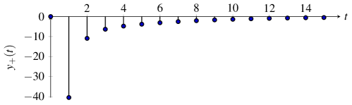
Figure 1: The output of the internally Hankel $2$-positive realization, $y_{+}(t)=({\mathcal{O}}(A_{+},b_{+})x_{0})(t)$, has a smaller variation than $x_{0}=(-40.5,0.9,0.015)^{\mathsf{T}}$ .

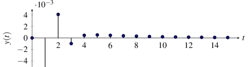
Figure 2: The output of the canonical controllable form realization eq. 19, $y(t)=({\mathcal{O}}(A,b)x_{0})(t)$, has a larger variation than $x_{0}=(-40.5,0.9,0.015)^{\mathsf{T}}$.

5.2 Impulse response analysis

Consider the following system, previously shown as an example in [22]:

$$G(z)=\frac{(z-0.22)(z-0.6)}{z^{3}(z-0.7)}$$

The transfer function $G(z)$ has a realization given by

$$A=\begin{pmatrix}0.7&1&0&0\\ 0&0&1&0\\ 0&0&0&1\\ 0&0&0&0\end{pmatrix}\,b=\begin{pmatrix}0\\ 1\\ -0.82\\ 0.132\end{pmatrix}\,c=\begin{pmatrix}1\\ 0\\ 0\\ 0\end{pmatrix}^{\mathsf{T}}$$ (20)

It can be verified that this realization has totally positive $A$ and ${\mathcal{O}^{4}}(A,c)$. Furthermore, since $A$ is upper triangular with band-width $1$, $A+\eta I$ is totally positive and $\textnormal{rank}(A+\eta I)$ is full for any $\eta>0$. Thus, by Corollary 4.1, the number of sign changes in the impulse response of $G(z)$ (and, hence, the number of extrema in its step response) is upper bounded by $\text{S}(b)=2$; this same upper bound was previously obtained by [22]. Figure 3 shows that the this bound is tight.

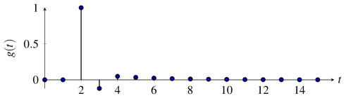
Figure 3: Impulse response of the system in eq. 20 has two zero crossings, which coincides with our derived upper bound.

However, in contrast to [22], our framework does not assume real poles or zeros. In particular, the modified transfer function

$$G_{m}(z)=\frac{(z-0.5+i)(z-0.5-i)}{z^{3}(z-0.7)},$$

can be realized with the same $A$ and $c$ as in eq. 20 and with $b=\begin{pmatrix}0&1&-1&1.25\end{pmatrix}^{\mathsf{T}}$, which again provides a tight upper bound on the variation of the impulse response.

Finally, note that by Proposition 2.5, there cannot be any $b$ such that ${\mathcal{C}}(A,b)$ is ${2\text{-positive}}$, because otherwise $(A,b,c)$ would be Hankel ${2\text{-positive}}$. This illustrates the importance of the irreducibility condition in Proposition 3.4.

6 Conclusion

Under the assumption of $k$-positive autonomous dynamics, this work has derived tractable conditions for which the controllability and observability operators are $k$-positive. These results have been used in two ways.

First, we introduced and studied the notion of internally Hankel $k$-positive systems, i.e., systems which are variation diminishing from past inputs with at most $k-1$ variations to future states to future outputs. It has been shown that these properties are tractable through internal positivity of the associated compound systems. In particular, internal Hankel $k$-positivity provides a means of studying external Hankel $k$-positivity with finite-dimensional tools. As a result, this systems class combines and extends two important system classes: (i) the celebrated class of internally positive systems ($k=1$) [10] and (ii) the class of relaxation systems [35] ($k=\infty$); the latter has also been shown to admit minimal internally Hankel totally positive realizations. Moreover, our results lay the groundwork for future work linking autonomous variation diminishing systems, as considered in [26, 1], with the theory of externally variation diminishing systems [17]. Finally, as a generalization of the case $k=1$ found in [28], a characterization of when an externally Hankel ${k\text{-positive}}$ system possesses a minimal internally Hankel ${k\text{-positive}}$ realization has been discussed. In future work, the characterizations for non-minimal realizations and realization algorithms shall be addressed. Noticeably, we have not introduced an internal notion for externally Toeplitz $k$-positive systems: this is a consequence of the non-separability of the Toeplitz operator. Thus, contrary to the standard definition of internal positivity, this suggests that the Hankel operator is a more natural object with which to associate internal positivity.

Second, we have developed a new framework for upper-bounding the number of sign changes in the impulse response of an LTI system. In particular, while the results of [22] are recovered in the case $k=\infty$, our framework allows considering generic $k$. In future work, we plan to address the conservatism of our analysis, its numerical numerical tractability, and the theoretical implication of the location of zeros. Further, we believe that a non-linear extension of our framework will be of timely importance. For instance, the cumulative difference between a step response and the output, called the (static) regret, is a common tractable measure in online learning [29] and adaptive control problems [21]. However, its meaningfulness depends on a small variability such as a small variance or a bounded variation.

References

• [1] R. Alseidi, M. Margaliot and J. Garloff “Discrete-Time $k$-Positive Linear Systems” In IEEE Transactions on Automatic Control 66.1, 2021, pp. 399–405 DOI: 10.1109/TAC.2020.2987285
• [2] B… Anderson, M. Deistler, L. Farina and L. Benvenuti “Nonnegative realization of a linear system with nonnegative impulse response” In IEEE Transactions on Circuits and Systems I: Fundamental Theory and Applications 43.2, 1996, pp. 134–142
• [3] Karl Johan Åström and Richard M Murray “Feedback systems: an introduction for scientists and engineers” Princeton university press, 2010
• [4] L. Benvenuti and L. Farina “A tutorial on the positive realization problem” In IEEE Transactions on Automatic Control 49.5, 2004, pp. 651–664 DOI: 10.1109/TAC.2004.826715
• [5] A. Berman and R. Plemmons “Nonnegative Matrices in the Mathematical Sciences” SIAM, 1994
• [6] Abraham Berman, Michael Neumann and Ronald J Stern “Nonnegative Matrices in Dynamic Systems” Wiley & Sons, 1989
• [7] T. Damm and L.. Muhirwa “Zero Crossings, Overshoot and Initial Undershoot in the Step and Impulse Responses of Linear Systems” In IEEE Transactions on Automatic Control 59.7, 2014, pp. 1925–1929 DOI: 10.1109/TAC.2013.2294616
• [8] S.M. Fallat and C.R. Johnson “Totally Nonnegative Matrices” Princeton University Press, 2011
• [9] Shaun Fallat, Charles R. Johnson and Alan D. Sokal “Total positivity of sums, Hadamard products and Hadamard powers: Results and counterexamples” In Linear Algebra and its Applications 520, 2017, pp. 242–259 DOI: https://doi.org/10.1016/j.laa.2017.01.013
• [10] L. Farina and S. Rinaldi “Positive linear systems: theory and applications”, Pure and applied mathematics (John Wiley & Sons) Wiley, 2000
• [11] Lorenzo Farina “On the existence of a positive realization” In Systems & Control Letters 28.4, 1996, pp. 219–226
• [12] Lorenzo Farina and Sergio Rinaldi “Positive Linear Systems: Theory and Applications” John Wiley & Sons, 2011
• [13] Miroslav Fiedler “Special matrices and their applications in numerical mathematics” Courier Corporation, 2008
• [14] Georg Frobenius “Über Matrizen aus nicht negativen Elementen” Königliche Gesellschaft der Wissenschaften, Göttingen, [s.a.]. ETH-Bibliothek Zürich, Rar 1524, 1912 DOI: 10.3931/e-rara-18865
• [15] C. Grussler, T. Damm and R. Sepulchre “Balanced truncation of $k$-positive systems”, 2020 eprint: arXiv:2006.13333
• [16] Christian Grussler and Anders Rantzer “On second-order cone positive systems”, arXiv:1906.06139, 2019 eprint: arXiv:1906.06139
• [17] Christian Grussler and Rodolphe Sepulchre “Variation diminishing linear time-invariant systems”, 2020 eprint: arXiv:2006.10030
• [18] Jean-Baptiste Hiriart-Urruty and Hai Yen Le “A variational approach of the rank function” In TOP 21.2, 2013, pp. 207–240 DOI: 10.1007/s11750-013-0283-y
• [19] Roger A. Horn and Charles R. Johnson “Matrix Analysis” Cambridge University Press, 2012
• [20] Samuel Karlin “Total positivity” Stanford University Press, 1968
• [21] N. Karlsson “Feedback Control in Programmatic Advertising: The Frontier of Optimization in Real-Time Bidding” In IEEE Control Systems Magazine 40.5, 2020, pp. 40–77 DOI: 10.1109/MCS.2020.3005013
• [22] M. El-Khoury, O.D. Crisalle and R. Longchamp “Discrete Transfer-function Zeros and Step-response Extrema” 12th Triennal Wold Congress of the International Federation of Automatic control. Volume 2 Robust Control, Design and Software, Sydney, Australia, 18-23 July In IFAC Proceedings Volumes 26.2, Part 2, 1993, pp. 537–542 DOI: https://doi.org/10.1016/S1474-6670(17)49000-8
• [23] Mario El-Khoury, Oscar D. Crisalle and Roland Longchamp “Influence of zero locations on the number of step-response extrema” In Automatica 29.6, 1993, pp. 1571–1574 DOI: https://doi.org/10.1016/0005-1098(93)90023-M
• [24] D.G. Luenberger “Introduction to Dynamic Systems: Theory, Models, and Applications” Wiley, 1979
• [25] David Luenberger “Introduction to Dynamic Systems: Theory, Models & Applications” John Wiley & Sons, 1979
• [26] Michael Margaliot and Eduardo D. Sontag “Revisiting Totally Positive Differential Systems: A Tutorial and New Results”, 2018 eprint: arXiv:1802.09590
• [27] James S. Muldowney “Compound matrices and ordinary differential equations” In Rocky Mountain J. Math. 20.4 Rocky Mountain Mathematics Consortium, 1990, pp. 857–872 DOI: 10.1216/rmjm/1181073047
• [28] Yoshito Ohta, Hajime Maeda and Shinzo Kodama “Reachability, Observability, and Realizability of Continuous-Time Positive Systems” In SIAM Journal on Control and Optimization 22.2, 1984, pp. 171–180
• [29] Francesco Orabona “A Modern Introduction to Online Learning”, 2019 eprint: arXiv:1912.13213
• [30] Oskar Perron “Zur Theorie der Matrices” In Mathematische Annalen 64.2, 1907, pp. 248–263 DOI: 10.1007/BF01449896
• [31] Anders Rantzer “Scalable control of positive systems” In European Journal of Control 24, 2015, pp. 72–80
• [32] N.. Son and D. Hinrichsen “Robust Stability of positive continuous time systems” In Numerical Functional Analysis and Optimization 17.5-6, 1996, pp. 649–659
• [33] D. Swaroop and D. Niemann “Some new results on the oscillatory behavior of impulse and step responses for linear time invariant systems” In Proceedings of 35th IEEE Conference on Decision and Control 3, 1996, pp. 2511–2512 vol.3 DOI: 10.1109/CDC.1996.573471
• [34] T. Tanaka and C. Langbort “The Bounded Real Lemma for Internally Positive Systems and H-Infinity Structured Static State Feedback” In IEEE Transactions on Automatic Control 56.9, 2011, pp. 2218–2223
• [35] Jan C Willems “Realization of systems with internal passivity and symmetry constraints” In Journal of the Franklin Institute 301.6 Elsevier, 1976, pp. 605–621