Efficient sampling of constrained high-dimensional theoretical spaces
with machine learning

Abstract

Models of physics beyond the Standard Model often contain a large number of parameters. These form a high-dimensional space that is computationally intractable to fully explore. Experimental constraints project onto a subspace of viable parameters, but mapping these constraints to the underlying parameters is also typically intractable. Instead, physicists often resort to scanning small subsets of the full parameter space and testing for experimental consistency. We propose an alternative approach that uses generative models to significantly improve the computational efficiency of sampling high-dimensional parameter spaces. To demonstrate this, we sample the constrained and phenomenological Minimal Supersymmetric Standard Models subject to the requirement that the sampled points are consistent with the measured Higgs boson mass. Our method achieves orders of magnitude improvements in sampling efficiency compared to a brute force search.

I Introduction

Models of physics beyond the Standard Model often feature many new parameters that are unknown a priori and may only be determined by experiment. However, experimental constraints are not trivial to apply, as they often are expressed in terms of weak-scale observables rather than the theory’s fundamental parameters. While it is often straightforward (if computationally expensive) to calculate the weak-scale observables from the parameters, the inverse problem is typically intractable. That is, weak scale constraints do not allow for a trivial reduction of the dimensionality of the theory space.

The standard approach is to numerically scan over the theoretical parameters and reject those that are not consistent with experimental data. However, the number of samples required for a brute-force search of the parameter space increases exponentially with its dimension. Thus, particle physicists studying models of new physics are often faced with a computationally intractable task. Out of pragmatism, one then restricts to a more tractable subset of parameters based on theoretical prejudice. The danger of this approach is that one may miss viable parameters that are both consistent with experimental observations and generate novel phenomenology.

The Minimal Supersymmetric Standard Model (MSSM) is a well-known example new physics model with a large number of free parameters ($\sim 100$); most of which are the masses and couplings of the supersymmetric partners of Standard Model particles [1]. This overwhelming dimensionality prohibits a fully general survey of the parameter space. Studies of the MSSM typically restrict to theoretically motivated subspaces [2, 3, 4, 5, 6, 7, 8, 9, 10, 11, 12, 13]. These include the 4+1 dimensional constrained MSSM (cMSSM) as well as the 19 dimensional phenomenological MSSM (pMSSM) [14, 15]. However, even these reduced spaces are difficult to scan using a brute-force search.

High dimensionality is not the only challenge when scanning the parameters of the MSSM. The fundamental parameters of the theory are defined at some high energy scale—e.g. the scale of a so-called Grand Unified Theory (GUT)—and must be evolved to the energy scale of the experiment. This evolution requires one to solve the coupled renormalization group equations for the high-scale parameters over many orders of magnitude to the weak scale. The computational cost of RGE running and calculating experimental observables for a single set of parameters is expensive, $\mathcal{O}(\text{second})$ for a modern CPU.

Many recent scans have incorporated machine learning in some capacity to decrease the computational burden of brute-force searching these spaces [12, 13, 7]. These use various machine learning models to learn the forward problem of determining weak scale properties given GUT scale parameters. This bypasses the need to perform RGE running and weak scale computations, however one is still faced with the challenge of doing a brute-force search over a high-dimensional parameter space. Machine learning models for the forward problem are thus only a constant improvement compared to the exponential dependence on the dimension of the space.

In this work, we introduce two methods to efficiently sample high-dimensional parameter spaces subject to constraints at the weak scale. We test these frameworks by sampling regions of the cMSSM and pMSSM parameter spaces that admit a Higgs mass consistent with its experimental value [16, 17]. The first uses a deep neural network to machine-learn the likelihood of an event satisfying this constraint and then samples this likelihood using Hamiltonian Monte Carlo (HMC). The second trains a generative model known as a normalizing flow. We then compare the performance of these frameworks to random sampling.

These methods allows us to directly and quickly generate points in the parameter space that admit a consistent Higgs mass. By solving the inverse problem of sampling GUT scale parameters given weak scale properties, we aim to minimize inefficiencies that arise in a brute-force search.

Our presentation is a proof of concept for these generative models and is encouraging for practical applications. For example, the ability to efficiently scan the MSSM parameter space makes it much easier to determine the high-scale parameters that are consistent with a new particle’s mass and width if a sparticle is discovered. Alternatively, a trained generative model may permit scans over parameters that are consistent with experimental observations to search for specific theoretical features that one may wish to study, for example: gauge coupling unification, a particular type of dark matter particle, or low fine tuning measures.

As a demonstration of the efficiency of the generative models, we scan the cMSSM and pMSSM parameter spaces for points that produce the Higgs mass and that saturate the observed dark matter relic density, requiring [18, 19]

$$\begin{array}[]{r@{{}}c@{{}}l}122~{}\text{GeV}<{}&m_{h}&{}<128~{}\text{GeV}\;,\\ 0.08<{}&\Omega_{\textrm{DM}}h^{2}&{}<0.14\;.\end{array}$$

In this study, the generative models have been trained for consistency with the Higgs mass, not the relic density. We compare a brute-force scan using random sampling to a generative model that has been trained to sample points that admit a consistent Higgs mass. We show that the generative models dramatically increase the sampling efficiency of this scan.

II Methods

II.1 Data Generation

The cMSSM contains 4 continuous parameters defined at the GUT scale and 1 discrete sign parameter. These are the universal scalar mass $m_{0}$, the universal gaugino mass $M_{1/2}$, universal trilinear coupling $A_{0}$, the ratio of Higgs vacuum expectation values $\tan\beta$, and the sign of $\mu$. The pMSSM is the most general subspace of the MSSM that admits first and second generation universality, no new sources of CP violation, and no flavor changing neutral currents [15]. The full list parameters of the pMSSM are listed as part of Table 2. Upon evolving these parameters to the weak scale, one is able to calculate observable quantities such as the Higgs mass and the dark matter thermal relic density, among others.

Our datasets are formed by uniform random sampling within bounded regions of the parameter space at the GUT scale. These bounds are listed for the cMSSM and the pMSSM in Table 1 and Table 2, respectively [2, 9], and are chosen to cover large volumes of the parameter space that are sensitive to modern collider experiments. For the cMSSM, we fix $\operatorname{sign}(\mu)=1$. We sample approximately $1.5\times 10^{6}$ datapoints in the cMSSM and approximately $1.95\times 10^{7}$ datapoints in the pMSSM. Once sampled, we calculate Higgs masses and relic densities with micrOMEGAs, which internally uses SoftSUSYv4.1.0 to perform RGE running [20, 21].

Parameter	Domain	Description
$m_{0}$	$[0,10]$ TeV	Universal scalar mass
$m_{1/2}$	$[0,10]$ TeV	Universal gaugino mass
$A_{0}$	$[-6m_{0},6m_{0}]$ TeV	Universal trilinear coupling
$\tan\beta$	$[1.5,50]$	Ratio of Higgs VEVs

Table 1: Parameter bounds in the cMSSM scan, following Ref. [2]. A uniform prior is used for all parameters except $A_{0}$, where we uniformly sample $A_{0}/m_{0}$.

Parameter	Domain	Description
$|M_{1}|$	$[.05,4]$ TeV	Bino mass
$|M_{2}|$	$[.1,4]$ TeV	Wino mass
$M_{3}$	$[.4,4]$ TeV	Gluino mass
$|\mu|$	$[.1,4]$ TeV	Bilinear Higgs mass
$|A_{t}|$	$[0,4]$ TeV	Trilinear top coupling
$|A_{b}|$	$[0,4]$ TeV	Trilinear bottom coupling
$|A_{\tau}|$	$[0,4]$ TeV	Trilinear $\tau$ coupling
$M_{A}$	$[.1,4]$ TeV	Pseudo-scalar Higgs mass
$m_{\tilde{L}_{1}}$	$[.1,4]$ TeV	1st gen. l.h. slepton mass
$m_{\tilde{e}_{1}}$	$[.1,4]$ TeV	1st gen. r.h. slepton mass
$m_{\tilde{L}_{3}}$	$[.1,4]$ TeV	3rd gen. l.h. slepton mass
$m_{\tilde{e}_{3}}$	$[.1,4]$ TeV	3rd gen. r.h. slepton mass
$m_{\tilde{Q}_{1}}$	$[.4,4]$ TeV	1st gen. l.h. squark mass
$m_{\tilde{u}_{1}}$	$[.4,4]$ TeV	1st gen. r.h. $u$-type squark mass
$m_{\tilde{d}_{1}}$	$[.4,4]$ TeV	1st gen. r.h. $d$-type squark mass
$m_{\tilde{Q}_{3}}$	$[.2,4]$ TeV	3rd gen. l.h. squark mass
$m_{\tilde{u}_{3}}$	$[.2,4]$ TeV	3rd gen. r.h. $u$-type squark mass
$m_{\tilde{d}_{3}}$	$[.2,4]$ TeV	3rd gen. r.h. $d$-type squark mass
$\tan\beta$	$[1,60]$	Ratio of Higgs VEVs

Table 2: Parameter bounds in the pMSSM scan, following Ref. [9]. A uniform prior is used for all parameters. “Left-handed” and “right-handed” are abbreviated by l.h. and r.h., respectively.

We apply the following two theoretical constraints: the parameters allow for consistent electroweak symmetry breaking and that all squared masses are positive. In addition to these, we also require that SoftSUSY converges. We do not require that the lightest supersymmetric particle is neutral, though this is the case for 90% of the cMSSM and 99% of the pMSSM parameter points with a consistent Higgs mass.

The theoretical uncertainty in Higgs mass calculations is significantly larger than its experimental uncertainty [22]. We take the uncertainty in the Higgs mass calculations to be $\sigma_{m_{h}}=3~{}$GeV for all points in the data set [2, 9].

II.2 Neural Network

To train the neural network, we assign all points in the dataset a likelihood

$$L(\theta)=\begin{cases}1&|m_{h}(\theta)-m_{h,\mathrm{exp}}|<\sigma_{m_{h}}\;,\\ 0&\text{otherwise}\;,\end{cases}$$ (II.1)

where the normalization constant is ignored. All data points that fail the theoretical constraints are assigned a likelihood of zero.

We use a deep neural network to learn the function $L(\theta)$ [23]. This has two benefits. First, it greatly reduces the time required to evaluate the likelihood of a point. Second, it provides a differentiable interpolation of $L(\theta)$. In the next section we show that HMC requires a significant number of likelihood evaluations as well as gradients of the likelihood. It thus utilizes the full potential of these benefits.

We train a deep neural network $\hat{L}(\theta)$ to minimize the usual L2 loss function

$$\mathcal{L}=|\hat{L}(\theta)-L(\theta)|^{2}\;.$$ (II.2)

We use a training, validation, and testing split of $0.7,0.15,0.15$ respectively for both datasets. Batch norm and dropout layers are used in between each hidden layer of the neural network. Backpropogation is performed using the ADAM optimizer [24].

Some of the pMSSM parameters in Table 2 span a disconnected range of positive and negative values, for example $M_{1}$, $M_{2}$ and $\mu$. We preprocess these parameters by shifting negative values to create a single continuous domain; for example, for $\mu$ we shift the negative values by 200 GeV. This has no physical significance and simply prepares the data for input into the neural network. We then standardize each feature. For the cMSSM dataset, we use the feature $A_{0}/m_{0}$ in place of $A_{0}$, as this feature is uniformly distributed.

II.3 Hamiltonian Monte Carlo

The Hamiltonian Monte Carlo method is a Markov chain Monte Carlo technique that allows distant proposals with high acceptance rates [25, 26]. First, we define an auxiliary momentum variable $p$, where each component is initially drawn from a normal distribution. Next, we define a potential energy function given by

$$V(\theta)=-\log(\hat{L}(\theta))\;.$$ (II.3)

The kinetic energy function takes the familiar form with unit mass $m=1$,

$$T=\frac{1}{2}p^{2}\;.$$ (II.4)

We then evolve the system from time $t=0$ to $t=\tau$ by solving Hamilton’s equations of motion

$$\frac{\mathop{}\!\mathrm{d}\theta_{i}}{\mathop{}\!\mathrm{d}t} =p_{i}\;, \frac{\mathop{}\!\mathrm{d}p_{i}}{\mathop{}\!\mathrm{d}t} =\frac{\nabla\hat{L}(\theta)}{\hat{L}(\theta)}\;.$$ (II.5)

We solve the equations of motion using the leap-frog algorithm so that energy is approximately conserved. We take $\theta(\tau)$ as a proposal to add to the Markov chain. The proposal is accepted with probability

$$P=\min\left(1,\frac{e^{-H(\theta(\tau),p(\tau))}}{e^{-H(\theta(0),p(0))}}\right)\;.$$ (II.6)

By energy conservation an analytic solution to the Hamilton equations should always yield probability 1. However, a rejection step is necessary because we solve these equations numerically. If $\theta(\tau)$ is rejected, then $\theta(0)$ is added to the Markov chain instead. In the limit of an infinite number of samples, the Markov chain converges to samples of the distribution $\hat{L}(\theta)$. We seed the Markov chain with a random positive sample from the dataset used to train the neural network. We set hard walls at the boundary of parameter space by setting the potential energy to infinity.

II.4 Normalizing Flows

It is difficult to draw samples from a complicated distribution, like the high-dimensional parameter spaces of the cMSSM and pMSSM. On the other hand, it is easy to draw samples from an equally high-dimensional Gaussian distribution. Normalizing flows is a technique that learns an invertible map $f$ from the simple distribution $p_{Z}$ to the challenging distribution $p_{Y}$. One then creates a set of samples from the challenging distribution by mapping easy-to-generate samples:

$$p_{Y}(y)=p_{Z}(f^{-1}(y))\left|\det\left(\frac{\partial f}{\partial y}\right)\right|^{-1}.$$ (II.7)

The function $f$ depends on a set of parameters $\Theta$ which are learned by maximizing the log likelihood of a training set, $\mathcal{X}$. The loss function for this training is thus

$$\mathcal{L}(\mathcal{X}) =-\sum_{y\in\mathcal{X}}\left(\log\left(p_{Z}(f^{-1}(y))\right)-\log\left|\det\left(\frac{\partial f}{\partial y}\right)\right|\right).$$

We construct $f$ to be the composition of $n$ successive maps, $f=f_{n}\circ\cdots\circ f_{1}$ [23]. Defining $z_{i+1}=f_{i}(z_{i})$ and identifying $y=z_{n+1}$ yields the loss function

$$\mathcal{L}(\mathcal{X}) =-\sum_{y\in\mathcal{X}}\left(\log\left(p_{Z}(z_{1})\right)-\sum_{i=1}^{n}\log\left|\det\left(\frac{\partial z_{i+1}}{\partial z_{i}}\right)\right|\right).$$

We choose the $f_{i}$ to be autoregressive transformations. This means that the parameters $\Theta^{k}_{i}$ that define the function $f_{i}$ acting on the $k^{\text{th}}$ feature $z_{i}^{k}$ depends only on the first $(k-1)$ features $z_{i}^{1},\cdots,z_{i}^{k-1}$. Explicitly,

$$z_{i+1}^{k}=f_{i}\bigl{(}z_{i}^{k}\,;\;\Theta_{i}^{k}(z_{i}^{1:k-1})\bigr{)}.$$

This structure ensures that the Jacobian matrix $\partial z_{i+1}/\partial z_{i}$ is lower triangular so that the determinant is simply the product of diagonal elements. Thus the function $f$ may be efficiently constructed in linear time.

The function $\Theta_{i}^{k}\left(z_{i}^{1:k-1}\right)$ can be represented efficiently with a Masked Autoencoder for Distribution Estimation (MADE) [27]. MADE networks turn off specific internal weights of the neural network so that the autoregressive property is enforced, allowing one neural network to output all model parameters rather than performing a sequential loop over features.

For our application, we choose $f_{i}$ to be rational-quadratic neural spline flows with autoregressive layers [28]. These are piece-wise monotonic functions defined as the ratio of two quadratic functions on the interval $[-B,B]$, with $K+1$ knots determining the boundaries between bins. Outside of this interval, the transformation is defined to be the identity. These transformations are parameterized by $3K-1$ parameters for each feature, which are $K$ bin heights, $K$ bin widths, and $K-1$ positive derivative values at the knots, as the derivatives are set to $1$ at $-B$ and $B$ to ensure a continuous derivative over the domain. Permutation layers are included between rational-quadratic transformation layers. We implement the normalizing flow using the Python package nflows [28].

III Results

We analyze the performance of these generative frameworks on the cMSSM and pMSSM datasets described above. The cMSSM is low dimensional and can be scanned relatively well with brute-force search. Thus, we view the cMSSM as a test for the generation methods and the pMSSM as a more practical application. We present the results for the neural network with HMC as well as the normalizing flow side by side. For each method, we generate a dataset of $4\times 10^{5}$ datapoints.

We present histograms of generated variables at the GUT scale to confirm that the distribution of theory parameters is not biased by our generative framework. We also present histograms of $m_{h}$ to ensure that our generative models sample within the band of permitted Higgs masses and $\Omega_{\textrm{DM}}h^{2}$ to provide evidence that the distribution of weak scale quantities match, as these are sensitive to higher order correlations in GUT scale parameters. Finally, we report sampling efficiencies, which are defined as the fraction of the dataset that satisfy a constraint. The hyperparameters used for the supervised neural network, Hamiltonian Monte Carlo, and normalizing flow are given in the Appendix for both datasets.

III.1 cMSSM

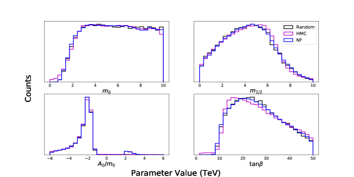
Figure 1: Histograms of cMSSM parameters that yield the experimental Higgs mass. We observe good agreement between the random sampling, HMC, and the flow model. Black: Data obtained through random sampling with a uniform prior and rejecting points that do not have a consistent Higgs mass. Magenta: data sampled with HMC. Blue: data sampled from the flow model. No rejection step is applied to generated samples.

In Figure 1, we compare histograms of GUT scale cMSSM parameters. For both generative models, we see very good agreement between the distribution of generated samples and the distribution of randomly sampled points after the Higgs mass constraint is applied. Next, we run the parameters to the weak scale in order to perform the combined search for $\Omega_{\textrm{DM}}h^{2}$ and $m_{h}$. In Figure 2, we show the distribution of Higgs masses for generated points and randomly sampled points with a rejection step applied. We see that the generative models typically sample within the band of permitted Higgs masses.

As an example application in this context, we show histograms of the dark matter relic density for these datasets in Figure 3. We see that the distribution over dark matter relic densities from the generative models appear to accurately reflect the same distribution in the dataset after the Higgs mass constraint is applied. We emphasize that because the RGEs are coupled, weak-scale quantities are generally sensitive to higher order correlations of the GUT scale parameters, and so matching weak-scale distributions is evidence of matching higher order correlations in the GUT scale parameters. This indicates that the $m_{h}$-constrained subspace has been accurately sampled, allowing for an exploration of additional constraints, such as relic density.

In Table 3, we compare various statistical properties of random sampling to those of our generative frameworks trained to satisfy the Higgs mass constraint. The first row shows the sampling efficiency with respect to the theoretical constraints mentioned in Section II.A. We see that samples from the generative models are more likely to pass these constraints, as points with a consistent Higgs mass necessarily satisfy the theoretical constraints. The second row shows the sampling efficiency with respect to the Higgs mass constraint. Predictably, the generative models have significantly higher sampling efficiencies than random sampling. We also see that the flow model slightly outperforms the HMC sampling method.

The third row shows the sampling efficiencies with respect to the combined Higgs mass and relic density constraint, where the generative models are still trained to only satisfy the Higgs mass constraint. As mentioned in the introduction, this simulates a scenario where one would like to study the effect of imposing a new constraint in addition to constraints that are already accounted for. Once again, we see that the generative models have much higher sampling efficiencies, resulting from the high probability that the samples pass the Higgs mass constraint. We see an increase in sampling efficiency of approximately an order of magnitude for both generative frameworks.

	Sampling Method
Constraint	Random	HMC${}_{m_{h}}$	NF${}_{m_{h}}$
Theory	$0.595$	$0.859$	$0.879$
$\text{Theory}\cap m_{h}$	$0.0389$	$0.723$	$0.796$
$\text{Theory}\cap m_{h}\cap\Omega_{\textrm{DM}}h^{2}$	$0.000222$	$0.00271$	$0.00456$

Table 3: Comparison of sampling efficiency in the cMSSM for several methods and several levels of constraints. We compare a brute force random scan (random), Hamiltonian MC of a neural network trained to learn the $m_{h}$ constraint (HMC${}_{m_{h}}$), and normalizing flows that incorporate the $m_{h}$ constraint (NF${}_{m_{h}}$). The constraints applied are theoretical consistency checks (see text), consistency with the experimental Higgs mass and consistency with the Higgs mass and the dark matter relic density $(\Omega_{\textrm{DM}}h^{2})$.

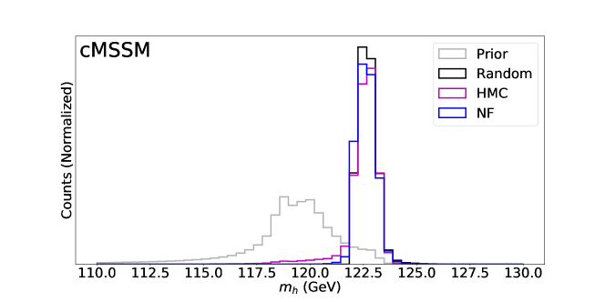
Figure 2: Histogram of Higgs masses in the cMSSM for different sampling methods. The generative models are seen to mostly sample points consistent with the Higgs mass constraint. Gray: data obtained through random sampling with a uniform prior. Black: the same randomly sampled data, but points that do not have a consistent Higgs mass are rejected. Magenta: data sampled with HMC. Blue: data sampled with the normalizing flow.

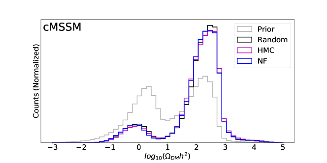
Figure 3: Histogram of dark matter thermal relic densities in the cMSSM for different sampling methods. We observe that the distributions of the generative models match the distribution of random sampling, providing evidence that the generative models are able to match higher order correlations in GUT scale parameters. Gray: data obtained through random sampling with a uniform prior. Black: the same randomly sampled data, but points that do not have a consistent Higgs mass are rejected. Magenta: data sampled with HMC. Blue: data sampled with the normalizing flow. Generative models have been trained to satisfy the Higgs mass constraint.

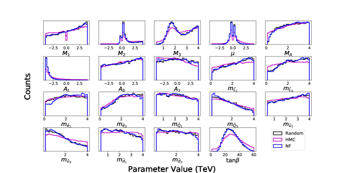
Figure 4: Histograms of pMSSM parameters that yield the experimental Higgs mass. We observe good agreement between random sampling, HMC, and the flow model. Black: Data obtained through random sampling with a uniform prior and rejecting points that do not have a consistent Higgs mass. Magenta: data sampled with HMC. Blue: data sampled from the flow model. No rejection step is applied to generated samples.

III.2 pMSSM

Differences between the generative models appear in the higher-dimensional pMSSM. In Figure 4, we compare histograms of GUT scale parameters sampled using brute-force search, HMC and the normalizing flow model. Despite the increased dimensionality, we find very good agreement in the distributions of all parameters at the GUT scale, though HMC has noticeable deviations in some parameters.

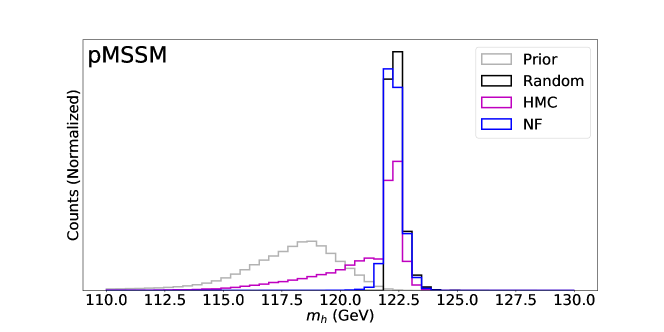
Figure 5: Histogram of Higgs masses in the pMSSM. The generative models are seen to mostly sample points consistent with the Higgs mass constraint. Gray: data obtained through random sampling with a uniform prior. Black: the same randomly sampled data, but points that do not have a consistent Higgs mass are rejected. Magenta: data sampled with HMC. Blue: data sampled with the normalizing flow.

Figures 5 and 6 present histograms of $m_{h}$ and $\Omega_{\textrm{DM}}h^{2}$ for the pMSSM. The generative models tend to sample in the band of allowed Higgs masses, with the normalizing flow model matching the brute-force scan well. The HMC samples have a long tail outside of this region towards smaller Higgs masses. We see general agreement with the true distribution of dark matter abundances for both generative frameworks, though the HMC samples do not match the brute-force distributions as well as those from the flow model.

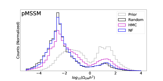
Figure 6: Histogram of dark matter thermal relic densities in the pMSSM. We observe that the distributions of the generative models match the distribution of random sampling, providing evidence that the generative models are able to match higher order correlations in GUT scale parameters. Gray: data obtained through random sampling with a uniform prior. Black: the same randomly sampled data, but points that do not have a consistent Higgs mass are rejected. Magenta: data sampled with HMC. Blue: data sampled with the normalizing flow. Generative models have been trained to satisfy the Higgs mass constraint.

Table 4 summarizes the performance of our sampling methods in the pMSSM. See Section III.1 for a detailed description of the quantities presented in the table. Despite the higher dimensionality of the pMSSM over the cMSSM, we find that generative models increase the sampling efficiency relative to a brute-force search by over two orders of magnitude. This is much greater than the increase seen in the cMSSM and is largely due to the poorer performance of a brute-force search in this space.

	Sampling Method
Constraint	Random	HMC${}_{m_{h}}$	NF${}_{m_{h}}$
Theory	$0.553$	$0.744$	$0.895$
$\text{Theory}\cap m_{h}$	$0.00095$	$0.319$	$0.663$
$\text{Theory}\cap m_{h}\cap\Omega_{\textrm{DM}}h^{2}$	$0.000022$	$0.00574$	$0.0141$

Table 4: Comparison of sampling efficiency in the pMSSM for several methods and several levels of constraints. Methods compared are brute force random scan, Hamiltonian MC of a neural network trained to learn the $m_{h}$ constraint (HMC${}_{m_{h}}$), and normalizing flows that incorporate the $m_{h}$ constraint (NF${}_{m_{h}}$). Constraints applied are theoretical consistency checks (see text), consistency with the experimental Higgs mass and consistency with the Higgs mass and the dark matter relic density $(\Omega_{\textrm{DM}}h^{2})$.

IV Conclusion

We implement two generative frameworks that utilize machine learning in order to increase the sampling efficiency of searches in supersymmetric parameter spaces. These sampling methods offer a more efficient way to search the high-dimensional parameter spaces in models of new particle physics. We compare these generative frameworks to the currently used method of a brute-force search, and have seen orders of magnitude of improvement in the sampling efficiency for both parameter spaces considered here. We show that our generative frameworks are able to sample the underlying data distribution without any evidence of bias or mode collapse.

In the cMSSM, both methods significantly outperformed random sampling, with the flow model slightly outperforming HMC. In the pMSSM the flow model significantly outperforms HMC. This is likely due to the larger dimensionality of the pMSSM. In addition to performance benefits, the flow model is also quicker to train and sample, making it clearly favorable to HMC. However, the HMC framework is more complementary to previous works, as it learns the forward problem of determining likelihoods and uses tested Monte Carlo algorithms to sample this likelihood.

Possibilities for future work include incorporating additional constraints into the generative model. In theory, there is no limit to the number of constraints that can be included into either generative model. However, forming an initial dataset for learning may be difficult when the constraints are very strict. A possible remedy is to train generative models with less restrictive constraints which are then used to produce sizable datasets of points that already satisfy many constraints. This new dataset could then be searched to form a training set for a generative model with increasingly restrictive constraints.

Given the ability of the generative machine learning models to efficiently explore high-dimensional parameter spaces, it will be interesting to apply the techniques described here to other problems. For instance, one may identify relations that explain why there is a ‘little hierarchy’ between the electroweak scale and the scale of soft parameters, which go beyond the focus point scenario [29]. In general, one may be able to identify manifolds of viable points in high-dimensional parameter sets, and explore their geometry.

We have shown promising results in subspaces of the MSSM parameter space. These results apply generally to any high-dimensional parameter space with constraints that are computationally expensive to verify. Another direction for future study may be applications to the parameter spaces of even higher-dimensional models of new physics. This includes potentially relaxing constraints built into the pMSSM parameter space, but could also include applications to non- supersymmetry (SUSY) theories. Finally, one could attempt to further tune the neural network structure and hyperparameters in order to achieve higher sample efficiency than was achieved in this work.

V Acknowledgements

The authors would like to thank Tim Cohen, Syris Norelli, Stephan Mandt and Babak Shahbaba. This material is based upon the work supported by the National Science Foundation Graduate Research Fellowship under Grant No. DGE-1321846. DW is supported by the Department of Energy Office of Science. PT is supported by DOE grant DE-SC/0008541. The work of MR is supported by the National Science Foundation under Grant No. PHY-1915005.

VI Appendix

We present the hyperparameters for our machine learning models in Table 5.

	Parameter	cMSSM	pMSSM
Supervised NN	Learning rate	$0.001$	$0.0001245$
	Hidden layers	$5$	$10$
	Nodes per layer	$49$	$154$
	Dropout	$0.5$	$0.0$
	Activation function	Sigmoid	Sigmoid
	Optimizer	ADAM	ADAM
	Batch size	$128$	$128$
	Epochs	$50$	$50$
pHMC	Step size	$0.025$	$0.008$
	Number of steps	$12$	$12$
	Mass	$1.0$	$1.0$
	Chain length	$5000$	$5000$
	Burn-in steps	$1000$	$1000$
	Number of chains	$100$	$100$
pNF	Num transforms	$3$	$3$
	Batch size	$1024$	$1024$
	Epochs	$300$	$300$
	$B$	$2.0$	$2.0$
	NN hidden features	$64$	$64$

Table 5: Hyperparameters used for the machine learning models for to the cMSSM and pMSSM datasets.

References

- [1] S. P. Martin, “A Supersymmetry primer,” Adv. Ser. Direct. High Energy Phys. 21 (2010) 1–153, arXiv:hep-ph/9709356.
- [2] T. Cohen and J. G. Wacker, “Here be dragons: the unexplored continents of the CMSSM,” Journal of High Energy Physics 2013 no. 9, (Sep, 2013) . http://dx.doi.org/10.1007/JHEP09(2013)061.
- [3] D. Ghosh, M. Guchait, S. Raychaudhuri, and D. Sengupta, “How constrained is the constrained MSSM?,” Physical Review D 86 no. 5, (Sep, 2012) . http://dx.doi.org/10.1103/PhysRevD.86.055007.
- [4] C. Han, K.-i. Hikasa, L. Wu, J. M. Yang, and Y. Zhang, “Status of CMSSM in light of current LHC Run-2 and LUX data,” Physics Letters B 769 (Jun, 2017) 470–476. http://dx.doi.org/10.1016/j.physletb.2017.04.026.
- [5] B. C. Allanach, “Impact of CMS Multi-jets and Missing Energy Search on CMSSM Fits,” Physical Review D 83 no. 9, (May, 2011) . http://dx.doi.org/10.1103/PhysRevD.83.095019.
- [6] O. Buchmueller, R. Cavanaugh, A. D. Roeck, M. J. Dolan, J. R. Ellis, H. Flächer, S. Heinemeyer, G. Isidori, J. Marrouche, D. M. Santos, K. A. Olive, S. Rogerson, F. J. Ronga, K. J. de Vries, and G. Weiglein, “The CMSSM and NUHM1 after LHC Run 1,” The European Physical Journal C 74 no. 6, (Jun, 2014) 2922. https://doi.org/10.1140/epjc/s10052-014-2922-3.
- [7] M. Bridges, K. Cranmer, F. Feroz, M. Hobson, R. Ruiz de Austri, and R. Trotta, “A coverage study of the CMSSM based on ATLAS sensitivity using fast neural networks techniques,” Journal of High Energy Physics 2011 no. 3, (Mar, 2011) . http://dx.doi.org/10.1007/JHEP03(2011)012.
- [8] M. Cahill-Rowley, J. L. Hewett, A. Ismail, and T. G. Rizzo, “Lessons and prospects from the pMSSM after LHC Run I,” Phys. Rev. D 91 (Mar, 2015) 055002. https://link.aps.org/doi/10.1103/PhysRevD.91.055002.
- [9] M. Cahill-Rowley, J. L. Hewett, A. Ismail, and T. G. Rizzo, “pMSSM Studies at the 7, 8 and 14 TeV LHC,” 2013.
- [10] G. Aad, B. Abbott, J. Abdallah, O. Abdinov, R. Aben, M. Abolins, O. S. AbouZeid, H. Abramowicz, H. Abreu, and et al., “Summary of the ATLAS experiment’s sensitivity to supersymmetry after LHC Run 1 — interpreted in the phenomenological MSSM,” Journal of High Energy Physics 2015 no. 10, (Oct, 2015) . http://dx.doi.org/10.1007/JHEP10(2015)134.
- [11] V. Khachatryan, A. M. Sirunyan, A. Tumasyan, W. Adam, E. Asilar, T. Bergauer, J. Brandstetter, E. Brondolin, M. Dragicevic, and et al., “Phenomenological MSSM interpretation of CMS searches in pp collisions at and 8 TeV,” Journal of High Energy Physics 2016 no. 10, (Oct, 2016) . http://dx.doi.org/10.1007/JHEP10(2016)129.
- [12] S. Caron, J. S. Kim, K. Rolbiecki, R. R. de Austri, and B. Stienen, “The BSM-AI project: SUSY-AI–generalizing LHC limits on supersymmetry with machine learning,” The European Physical Journal C 77 no. 4, (Apr, 2017) 257. https://doi.org/10.1140/epjc/s10052-017-4814-9.
- [13] B. Kronheim, M. Kuchera, H. Prosper, and A. Karbo, “Bayesian neural networks for fast SUSY predictions,” Physics Letters B 813 (Feb, 2021) 136041. http://dx.doi.org/10.1016/j.physletb.2020.136041.
- [14] A. H. Chamseddine, R. Arnowitt, and P. Nath, “Locally Supersymmetric Grand Unification,” Phys. Rev. Lett. 49 (Oct, 1982) 970–974. https://link.aps.org/doi/10.1103/PhysRevLett.49.970.
- [15] MSSM Working Group Collaboration, A. Djouadi et al., “The Minimal supersymmetric standard model: Group summary report,” in GDR (Groupement De Recherche) - Supersymetrie. 12, 1998. arXiv:hep-ph/9901246.
- [16] G. Aad, T. Abajyan, B. Abbott, J. Abdallah, S. Abdel Khalek, A. Abdelalim, O. Abdinov, R. Aben, B. Abi, M. Abolins, and et al., “Observation of a new particle in the search for the Standard Model Higgs boson with the ATLAS detector at the LHC,” Physics Letters B 716 no. 1, (Sep, 2012) 1–29. http://dx.doi.org/10.1016/j.physletb.2012.08.020.
- [17] S. Chatrchyan, V. Khachatryan, A. Sirunyan, A. Tumasyan, W. Adam, E. Aguilo, T. Bergauer, M. Dragicevic, J. Erö, C. Fabjan, and et al., “Observation of a new boson at a mass of 125 GeV with the CMS experiment at the LHC,” Physics Letters B 716 no. 1, (Sep, 2012) 30–61. http://dx.doi.org/10.1016/j.physletb.2012.08.021.
- [18] D. N. Spergel, L. Verde, H. V. Peiris, E. Komatsu, M. R. Nolta, C. L. Bennett, M. Halpern, G. Hinshaw, N. Jarosik, A. Kogut, and et al., “First‐Year Wilkinson Microwave Anisotropy Probe ( WMAP ) Observations: Determination of Cosmological Parameters,” The Astrophysical Journal Supplement Series 148 no. 1, (Sep, 2003) 175–194. http://dx.doi.org/10.1086/377226.
- [19] C. L. Bennett, D. Larson, J. L. Weiland, N. Jarosik, G. Hinshaw, N. Odegard, K. M. Smith, R. S. Hill, B. Gold, M. Halpern, E. Komatsu, M. R. Nolta, L. Page, D. N. Spergel, E. Wollack, J. Dunkley, A. Kogut, M. Limon, S. S. Meyer, G. S. Tucker, and E. L. Wright, “NINE-YEAR WILKINSON MICROWAVE ANISOTROPY PROBE ( WMAP ) OBSERVATIONS: FINAL MAPS AND RESULTS,” The Astrophysical Journal Supplement Series 208 no. 2, (Sep, 2013) 20. https://doi.org/10.1088/0067-0049/208/2/20.
- [20] G. Belanger, F. Boudjema, A. Pukhov, and A. Semenov, “micrOMEGAs : a tool for dark matter studies,” 2010.
- [21] B. Allanach, “SOFTSUSY: A program for calculating supersymmetric spectra,” Computer Physics Communications 143 no. 3, (Mar, 2002) 305–331. http://dx.doi.org/10.1016/S0010-4655(01)00460-X.
- [22] P. Athron, J.-h. Park, T. Steudtner, D. Stöckinger, and A. Voigt, “Precise Higgs mass calculations in (non-)minimal supersymmetry at both high and low scales,” Journal of High Energy Physics 2017 no. 1, (Jan, 2017) . http://dx.doi.org/10.1007/JHEP01(2017)079.
- [23] C. M. Bishop, Pattern Recognition and Machine Learning (Information Science and Statistics). Springer-Verlag, Berlin, Heidelberg, 2006.
- [24] D. P. Kingma and J. Ba, “Adam: A Method for Stochastic Optimization,” arXiv:1412.6980 [cs.LG].
- [25] R. M. Neal, “MCMC using Hamiltonian dynamics,” 2012.
- [26] M. Betancourt, “A Conceptual Introduction to Hamiltonian Monte Carlo,” 2018.
- [27] G. Papamakarios, T. Pavlakou, and I. Murray, “Masked Autoregressive Flow for Density Estimation,” arXiv:1705.07057 [stat.ML].
- [28] C. Durkan, A. Bekasov, I. Murray, and G. Papamakarios, “Neural Spline Flows,” arXiv:1906.04032 [stat.ML].
- [29] J. L. Feng, K. T. Matchev, and T. Moroi, “Focus points and naturalness in supersymmetry,” Phys. Rev. D 61 (2000) 075005, arXiv:hep-ph/9909334.
- MSSM
- Minimal Supersymmetric Standard Model
- pMSSM
- phenomenological MSSM
- cMSSM
- constrained MSSM
- SUSY
- supersymmetry
- GUT
- Grand Unified Theory
- HMC
- Hamiltonian Monte Carlo
- RGE
- renormalization group equation