Macroscopic Fluctuations Emerge in Balanced Networks with Incomplete Recurrent Alignment

Abstract

Networks of strongly-coupled neurons with random connectivity exhibit chaotic, asynchronous fluctuations. In a previous study, we showed that when endowed with an additional low-rank connectivity consisting of the outer product of orthogonal vectors, these networks generate large-scale coherent fluctuations. Although a striking phenomenon, that result depended on a fine-tuned choice of low-rank structure. Here we extend that result by generalizing the theory of excitation-inhibition balance to networks with arbitrary low-rank structure and show that low-dimensional variability emerges intrinsically through what we call “incomplete recurrent alignment”. We say that a low-rank connectivity structure exhibits incomplete alignment if its row-space is not contained in its column-space. In the generic setting of incomplete alignment, recurrent connectivity can be decomposed into a “subspace-recurrent” component and an “effective-feedforward” component. We show that high-dimensional, microscopic fluctuations are propagated via the effective-feedforward component to a low-dimensional subspace where they are dynamically balanced by macroscopic fluctuations. We present biologically plausible examples from excitation-inhibition networks and networks with heterogeneous degree distributions. Finally, we define the alignment matrix as the overlap between left- and right-singular vectors of the structured connectivity, and show that the singular values of the alignment matrix determine the amplitude of low-dimensional variability, while its singular vectors determine the structure. Our work shows how low-dimensional fluctuations can emerge generically in strongly-coupled networks with low-rank structure. Furthermore, by generalizing excitation-inhibition balance to arbitrary low-rank structure our work may find relevance in any setting with strongly interacting units, whether in biological, social, or technological networks.

Introduction

The dynamic balance of excitation (E) and inhibition (I) is a paradigmatic theory for describing the activity of neocortical networks (van Vreeswijk and Sompolinsky, 1996, 1998; Brunel, 2000; Renart et al., 2010a). The theory describes how recurrent interactions generate asynchronous irregular firing activity which is typically observed in the cortex across many species, especially in awake, active states of behavior (Softky and Koch, 1993; Ecker et al., 2010, 2014; Cohen and Kohn, 2011; Doiron et al., 2016). The E-I balance network model is driven by strong feed-forward excitation, and strong recurrent connectivity, dominated by inhibition, is necessary in order to balance that input. The result is that the average activity of E and I populations dynamically balance the mean synaptic input, enabling fluctuations to propagate asynchronously. The resulting networks can account for various empirical observations of cortical activity, including not only irregular firing but also low pairwise correlations (Renart et al., 2010a) and broad firing-rate distributions (Roxin et al., 2011). Furthermore, balanced networks perform fast-tracking of external input which can underly predictive coding (Kadmon et al., 2020), and they are capable of amplifying input feature selectivity (Hansel and van Vreeswijk, 2012; Pehlevan and Sompolinsky, 2014) and generating stable patterns of activity for associative memory (van Vreeswijk and Sompolinsky, 2005; Roudi and Latham, 2007; Mongillo et al., 2018).

Many qualitative aspects of the dynamics of excitation-inhibition balance can be understood by studying simpler firing-rate models (Wilson and Cowan, 1972). Firing rate models of randomly connected excitatory and inhibitory populations with strong interactions and strong feed-forward input exhibit a dynamic cancelation of the mean input at the population level (Harish and Hansel, 2015; Kadmon and Sompolinsky, 2015), similarly to the spiking models. The resulting state is chaotic and asynchronous, due to asymmetric random connections(Sompolinsky et al., 1988).

It had been a longstanding question whether such randomly connected networks could intrinsically generate large-scale coherent fluctuations. We previously showed that when randomly connected networks are endowed with additional low-rank connectivity of a particular structure, fluctuations emerge that are shared coherently across the entire network (Landau and Sompolinsky, 2018). Specifically, connectivity structure consisting of outer-products of orthogonal pairs embed a purely feedforward structure into the recurrent network such that fluctuations along the row-space are propagated to the column-space, yielding shared variability in the column-space, without generating feedback that would either supress fluctuations or drive saturation. The same qualitative phenomenon was studied also by Darshan et al (Darshan et al., 2018) and Hayakawa and Fukai Hayakawa and Fukai (2020).

In the current work we study a broader framework of what we refer to as “incomplete recurrent alignment,” of which an orthogonal outer-product is one limiting case. In order to develop our theory of incomplete recurrent alignment, we generalize the theory of excitation-inhibition balance to networks with arbitrary low-rank structure. A number of recent studies have explored the dynamics of networks with low-rank structured connectivity in addition to a random component of connectivity, yet these have all focused on weakly-coupled low-rank structure (Rivkind and Barak, 2017; Mastrogiuseppe and Ostojic, 2018). We show that embuing random networks with strong low-rank connectivity yields a natural generalization of excitation-inhibition balance: a regime of dynamic balance in which strong input to a low-dimensional subspace is canceled without fine-tuning, and fluctuations can emerge in the orthogonal complement.

Using our generalized dynamic balance formalism, we show that incomplete recurrent alignment genereates macroscopic fluctuations. We say that a strongly-coupled recurrent network has incomplete alignment if the row-space of its structured connectivity is not entirely contained in its column-space. We decompose the structrued connectivity into a “subspace recurrent” component, through which macroscopic activity in the column-space is able to dynamically balance its input, and an “effective-feedforward” component, through which microscopic fluctuations in the orthogonal subspace serve as a source of fluctuating input to the macroscopic dynamics in the column-space.

In the general case of incomplete alignment, this fluctuating source from the orthogonal subspace is dynamically balanced by macroscopic fluctuations in the column-space, which we refer to as the “balance subspace”. This balancing of fluctuations is analogous to the way a balanced network cancels shared fluctuations received from external sources (Renart et al., 2010b), except that here the source of the fluctuating input is recurrent. The larger the extent of misalignment, the larger the macroscopic fluctuations that arrise in order to achieve balance. Our theory yields a second-order balance equation for intrinsically generated macroscopic fluctuations, and we show how the macroscopic correlation structure is fully determined by the overlap matrix between left- and right-singular vectors of the structured connectivity, while the time-course of fluctuations is inherited from the time-course of microscopic fluctuations.

In Section I we introduce the model. In Section II we present the decomposition into macroscopic order parameters that reside in the low-dimensional “balance subspace” on the one hand, and microscopic degrees of freedom in the orthogonal subpsace on the other. We show that strong low-rank connectivity yields dynamic balance – a linear equation for the macroscopic firing rates in the balance subspace, and microscopic chaotic fluctuations in the orthogonal subspace. In Section III we show that incomplete alignment of the low-rank connectivity projects the microscopic fluctuations into the balance subspace yielding amplified shared variability. We derive expressions for the amplitude, spatial structure and timescale of this variability. Finally, in Section IV we study two concrete examples of biologically relevant incomplete alignment, excitatory-inhibitory networks with degenerate synaptic weight parameters (as previously studied in (Helias et al., 2014)), and networks with heterogeneous out-degrees.

Results

I Model

We study a network of $N$ firing-rate neurons with a connectivity matrix consisting of structured and random components. The structured component, $\mathbf{M}$, is given by a rank $D$ matrix, where $D$ is finite in the large $N$ limit, and the random component $\mathbf{J}$ has i.i.d. components assumed for simplicity to be Gaussian. Individual elements of both components of the connectivity scale as $\frac{1}{\sqrt{N}}$. Explicitly, we write the structured connectivity matrix in reduced singular value decomposition (SVD) form:

$$\mathbf{M}=\frac{1}{\sqrt{N}}\mathbf{U}\boldsymbol{\Sigma}\mathbf{V}^{T}$$ (1)

where both $\mathbf{U}$ and $\mathbf{V}$ are $N$-by-$D$ matrices with $O\left(1\right)$ components and orthogonal columns of norm $\sqrt{N}$, i.e. $\mathbf{U}^{T}\mathbf{U}=\mathbf{V}^{T}\mathbf{V}=N\mathbf{I}_{DxD}$ (notice that we adopt here a scaling of U and V that differs from the standard SVD convention). $\boldsymbol{\Sigma}$ is a diagonal $D$-by-$D$ matrix with $O\left(1\right)$ positive elements, $\sigma_{k}$.

We define the random component, $\mathbf{J}$, whose elements are sampled i.i.d. from $J_{ij}\sim\mathcal{N}\left(0,\frac{g^{2}}{N}\right)$ with a “gain” parameter $g=O(1)$. For simplicity, we assume that the elements of $\mathbf{J}$ are drawn independently of the structure of $\mathbf{U}$ and $\mathbf{V}$, i.e., we assume that $\frac{1}{N}\mathbf{V}^{T}\mathbf{J}^{k}\mathbf{U}\approx 0$ for all $k\geq 1$Schuessler et al. (2020).

The dynamics of the inputs (Fig 1A) are driven by strong external drive, $\sqrt{N}\mathbf{f},$with $f_{i}\sim O\left(1\right)$, and given by:

$$\dfrac{\mathrm{d}\mathbf{h}}{\mathrm{d}t}=-\mathbf{h}+\left(\mathbf{M}+\mathbf{J}\right)\mathbf{r}+\sqrt{N}\mathbf{f}$$ (2)

where the firing rates of individual neurons are given by $r_{i}=\text{$\phi\left(h_{i}\right)$}$, an instantaneous, sigmoidal non-linearity of the inputs. Unless otherwise mentioned, simulations and numerical calculations in this paper use $\phi\left(h)\right)=\tanh\left(h)\right)$, which can be thought of as the change in firing rate relative to some baseline.

As displayed in Figure 1A, the network structure can be understood schematically: $\mathbf{v}_{k}$, i.e. the $k$th right-singular vector of $\mathbf{M}$, performs a read-out of the network activity; this readout scaled by $\sigma_{k}$ and fed back into the network along the corresponding left-singular vector $\mathbf{u}_{k}$ (Fig 1A).

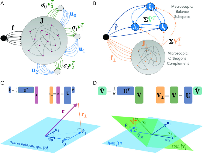
Figure 1: Model Dynamics and Schematic. (A) Schematic representation of network structure with external drive vector, $\mathbf{f}$, random recurrent connectivity, $\mathbf{J}$, and structured recurrent connectivity represented as a read-out along each right-singular vector, $\mathbf{v}_{k}$, scaled by $\sigma_{k}$, and fedback to the network along left-singular vector, $\mathbf{u}_{k}$. (B) Balance subspace decomposition. Schematic representing the decomposition into balance subspace and the orthogonal complement. The subspace recurrence within the balance subspace is given by $\boldsymbol{\Sigma}\hat{\mathbf{V}}^{T}$. The effective-feedforward connectivity from the orthogonal complement to the balance subspace is given by $\boldsymbol{\Sigma}\mathbf{V}_{\perp}^{T}$, which is $0$ in the fully aligned case. (C) Balance subspace decomposition for population vector of firing rates, $\mathbf{r}$. Top: Equations defining $\hat{\mathbf{r}}$ and $\mathbf{r}_{\perp}$. Bottom: Geometric visualization of the balance subspace decomposition.The projection into the balance subspace is given by the compontents, $\hat{r}_{k}$, along each left-singular vector, $\mathbf{u}_{k}$. The projection onto the orthgonal complement is $\mathbf{r}_{\perp}$. The same definitions apply for the dynamical variables, $\mathbf{h}$, and the external drive, $\mathbf{f}$. (D) Balance subspace decomposition of the connectivity structure, defining the alignment matrix, $\hat{\mathbf{V}}$. Top: Equations defining $\hat{\mathbf{V}}$ and $\mathbf{V}_{\perp}$. The same definitions as in (C) are applied to a matrix of $D$ column vectors, each of length $N$. Bottom: Geometrix visualization of incomplete alignment. The span of the columns of $\mathbf{V}$ may generally not be constrained to the balance subspace. The right-singular vector, $\mathbf{v}_{0}$, is projected onto the balance subspace where its component along each left-singular vector, $\mathbf{u}_{0}$ and $\mathbf{u}_{1}$, define the matrix elements $\hat{V}_{00}$ and $\hat{V_{10}}$, respectively. The projection of $\mathbf{v}_{0}$ onto the orthogonal complement defines, $\mathbf{v}_{0}^{\perp}$, the first column of $\mathbf{V}_{\perp}$. Similarly for all right-singular vectors, not shown. If the connectivty structure is “fully aligned”, then the span of $\mathbf{V}$ is identical to the span of $\mathbf{U}$ and the right-singular vectors are obtained from the left-singular vectors by rotation and reflection, such that the alignment matrix, $\hat{\mathbf{V}}$, is orthonormal.

II Balance Subspace Decomposition and the Alignment Matrix

The span of the left-singular vectors, $\mathbf{u}_{k}$, i.e the column-space of the structured connectivity $\mathbf{M}$, defines a distinct subspace. Both the structured and random components of connectivity have strong single synapses, i.e. they are $O\left(\frac{1}{\sqrt{N}}\right)$. However, we observe that the SVD of the random component will yield singular values of $O\left(\frac{1}{N}\right)$, such that any vector of $O\left(1\right)$ firing rates will yield only $O\left(1\right)$ input via the random component. On the other hand, the structured component of connectivity can yield $O\left(\sqrt{N}\right)$ input along the columns of $\mathbf{U}$. Therefore, the subspace spanned by the columns of $\mathbf{U}$ can receive strong recurrent inputs that will drive saturation unless they are balanced, and it will define the macroscopic order parameters of our system.

We call the column-space of the structured connectivity the “balance subspace”. We define the decomposition into the balance subspace and its orthogonal complement: for any $N$-dimensional vector or matrix with $N$-dimensional column-space, $\mathbf{X}$, we write $\mathbf{X}=\mathbf{X}_{\parallel}+\mathbf{X}_{\perp}$, where $\mathbf{X}_{\parallel}=\frac{1}{N}\mathbf{U}\mathbf{U}^{T}\mathbf{X}$ is the projection in the balance subspace, and $\mathbf{X}_{\perp}=\left(\mathbf{I}-\frac{1}{N}\mathbf{U}\mathbf{U}^{T}\right)\mathbf{X}$ is the projection in the orthogonal subspace.

We study the components in the balance subspace relative to the columns of $\mathbf{U}$, that is we write $\mathbf{X}_{\parallel}=\mathbf{U}\hat{\mathbf{X}}$ with

$$\hat{\mathbf{X}}\equiv\frac{1}{N}\mathbf{U}^{T}\mathbf{X}$$ (3)

Figure 1C displays the geometry of this decomposition for the population firing rate vector, $\mathbf{r}=\mathbf{U}\hat{\mathbf{r}}+\mathbf{r}_{\perp}$. We will similarly decompose the input currents, $\mathbf{h}$, into $\mathbf{U}\hat{\mathbf{h}}+\mathbf{h}_{\perp}$.

Additionally, as will be motivated in the following section, we will decompose the matrix of right-singular vectors, $\mathbf{V}=\mathbf{U}\hat{\mathbf{V}}+\mathbf{V}_{\perp}$, introducing the “alignment matrix”, $\hat{\mathbf{V}}$, between the column-space and row-space of the structured connectivity,

$$\hat{\mathbf{V}}=\frac{1}{N}\mathbf{U}^{T}\mathbf{V}$$ (4)

The alignment matrix is the $D$-by-$D$ matrix consisting of the overlap of each right-singular vector of the structured connectivity along each left-singular vector. Figure 1D displays the geometry of the two overlapping hyperplanes, given by the span of left- and right-singular vectors

Importantly, if the right-singular vectors are all contained in the balance subspace, i.e. if the row-space is entirely contained in the column-space, thenthe orthogonal complement is null ($\mathbf{V}_{\perp}=\mathbf{0}$). We refer to this condition as “full recurrent alignment”. Full recurrent alignment is obtained if an only if $\hat{\mathbf{V}}^{T}\hat{\mathbf{V}}=\mathbf{I}_{DxD}$, i.e. if the alignment matrix is orthonormal.

We will assume the external drive is aligned with the balance subpsace so that $\mathbf{f}=\mathbf{U}\hat{\mathbf{f}}$.

II.1 Balance Subspace Dynamics

We decompose the dynamics 2, and first study the the dynamics in the balance subspace, which are the macroscopic order parameters of the network. To do so we apply the above decomposition (Eqn3) on the structured connectivity, $\mathbf{M}$, Eq. 1, in order to write $\hat{\mathbf{M}}=\frac{1}{\sqrt{N}}\mathbf{\boldsymbol{\Sigma}}\mathbf{V}^{T}$. We note that by construction, $\mathbf{M}_{\perp}=0$, since $\mathbf{M}$ projects entirely into the balance subspace.

We use the alignment matrix, $\hat{\mathbf{V}}$, and the orthogonal complement ,$\mathbf{V}_{\perp}$, to further decompose $\mathbf{M}$, giving $\hat{\mathbf{M}}=\frac{1}{\sqrt{N}}\boldsymbol{\Sigma}\hat{\mathbf{V}}^{T}\mathbf{U}^{T}+\frac{1}{\sqrt{N}}\boldsymbol{\Sigma}\mathbf{V}_{\perp}^{T}$. The first term drive the “subspace-recurrent” component of the input, which is due to activity within the balance subspace, while the second term drives the “effective-feedforward” input, which is due to activity in the orthogonal complement.

Given population firing rates, $\mathbf{r}=\mathbf{U}\mathbf{\hat{r}}+\mathbf{r}_{\perp}$, the subspace-recurrent input is $\sqrt{N}\boldsymbol{\Sigma}\hat{\mathbf{V}}^{T}\hat{\mathbf{r}}$ and the effective-feedforward input is $\frac{1}{\sqrt{N}}\boldsymbol{\Sigma}\mathbf{V}_{\perp}^{T}\mathbf{r}_{\perp}$. Projecting the dynamics (Eqn 2) onto the balance subspace yields the macroscopic dynamcis:

$$\dfrac{\mathrm{d}\hat{\mathbf{h}}}{\mathrm{d}t}=-\hat{\mathbf{h}}+\sqrt{N}\left(\boldsymbol{\Sigma}\hat{\mathbf{V}}^{T}\hat{\mathbf{r}}+\hat{\mathbf{f}}\right)+\frac{1}{\sqrt{N}}\boldsymbol{\Sigma}\mathbf{V}_{\perp}^{T}\mathbf{r}_{\perp}+O\left(\frac{1}{\sqrt{N}}\right)$$ (5)

where the $O\left(\frac{1}{\sqrt{N}}\right)$ term is the contribution from the random connectivity, $\mathbf{J}$, onto the balance subspace, which we have ignored. Note that the effective-feedforward contribution via $\mathbf{V}_{\perp}$ is of $O\left(1\right)$.

These macroscopic dynamics admit a balanced fixed point governed by $D$ linear equations:

$$\boldsymbol{\Sigma}\hat{\mathbf{V}}^{T}\hat{\mathbf{r}}^{*}+\hat{\mathbf{f}}=O\left(\frac{1}{\sqrt{N}}\right)$$ (6)

Note that the effective-feedforward input does not contribute to the balance fixed point up to leading order. It will nevertheless have an impact on the macroscopic fluctuations around the fixed point as we shall see below.

The linear balance equations and their solution generalize the $2$-dimensional E-I balance equations to arbitrary low-rank structure and emphasize that they have a natural basis in the columns of $\mathbf{U}$, i.e. the left singular vectors of the structured component of connectivity. Moreover these balance equations are independent of the structure of $\mathbf{U}$, depending only on the singular values and the alignment matrix $\hat{\mathbf{V}}$.

Finally, we note that in general the balance equations may or or may not have an obtainable solution (e.g., consistent with non-saturating local rates). In the following we will assume that the local firing activations and external inputs are normalized such that the balance equations yield a feasible solution, see Appendix Appendix A - Self-Consistency of the Balance Solution and Appendix B - Mean-Field Theory in the Orthogonal Subspace.

II.2 Microscopic dynamics

We now consider the dynamics in the orthogonal complement, by projecting the full dynamics (Eqn 2) via $\mathbf{h}_{\perp}=\left(\mathbf{I}-\frac{1}{N}\mathbf{U}\mathbf{U}^{T}\right)\mathbf{h}$ (recall that we assume that the external drive is contained in the balance subspace):

$$\dfrac{\mathrm{d}\mathbf{h}_{\perp}}{\mathrm{d}t}=-\mathbf{h}_{\perp}+\mathbf{J}_{\perp}\mathbf{r}$$ (7)

Due to the random connectivity, $\mathbf{J}_{\perp}$, These microscopic dynamics can be described by a Gaussian dynamic mean-field theory which we detail in the Appendix following Kadmon and Sompolinsky (2015). The mean-field theory predicts that for sufficiently strong random connectivity these equations will generate asynchronous chaotic dynamics. The order parameter of the chaotic state is the mean single-neuron autocorrelation function $C\left(\tau\right)\equiv\left\langle\delta r_{i}\left(t\right)\delta r_{i}\left(t+\tau\right)\right\rangle$. The implicit differential equation governing $C(\tau)$ is derived from the dynamic mean-field theory and given in Appendix Appendix B - Mean-Field Theory in the Orthogonal Subspace. Note that these microscopic dynamics and the resulting mean-field theory depend on the macroscopic dynamics in the balance subspace, $\hat{\mathbf{h}}$. Both the fixed point values of $\hat{\mathbf{h}}$ and the autocorrelation, $C\left(\tau\right)$, must be consistent with the firing rates determined by the balance equations. We solve the dynamic mean-field theory and find a good match between simulation and theory (SI Fig 1).

As mentioned above, we assume that the balance firing rates given by Eqn 6 yield a non-saturating solution such that sufficiently strong random connectivity will yield chaotic microscopic dynamics (See Appendix Appendix A - Self-Consistency of the Balance Solution).

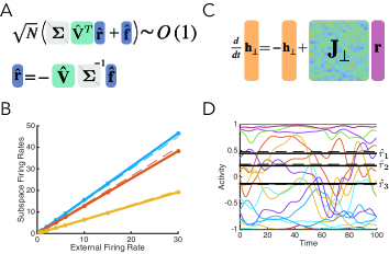
Figure 2: Dynamic Balance in Networks with Low-Rank Structure. (A) Top: Balance requirement for the cancelation of potentially large ($\sqrt{N}$) input into the balance subspace. Bottom: Solution to $D$ linear balance equations in the case where the column-space and row-space are fully aligned (alignment matrix, $\hat{\mathbf{V}}$, is orthonormal). (B) Balance subspace time-average firing rates, $\left\langle\hat{r}_{k}\right\rangle$, vs overall scaling factor of external firing rate, solid lines are the simulations which match closely with the prediction from linear balance equations (A) shown in dotted lines (C) Dynamics of the microscopic degrees of freedom in the orthogonal complement. (D) Sample activity trace. Colored lines are individual neuron firing rates, $r_{i}\left(t\right)$, displaying chaotic fluctuations. Black lines are the balance subspace firing rates, $\hat{r}_{k}\left(t\right)$, with simulations in solid lines and theory in dashed lines. ((B) employed a rectified-linear non-linearity $\phi\left(h\right)\equiv\left\lfloor h\right\rfloor_{+}$)

III Incomplete Alignment Amplify Fluctuations

In this section we assume a network in the chaotic balanced state described above. In this state, the macroscopic balance subspace firing rates, $\hat{\mathbf{r}}$ (defined via 3) satisfy the balance equations (Eqn 6), and are thus constant to leading order.

In this section we show that incomplete alignment amplifies macroscopic fluctuations in the balance subspace, $\delta\hat{\mathbf{r}}\left(t\right)\equiv\hat{\mathbf{r}}\left(t\right)-\left\langle\hat{\mathbf{r}}\right\rangle$. These are quantified by the $D$-by-$D$ matrix of covariance functions:

$$\hat{\mathbf{C}}\left(\tau\right)\equiv\left\langle\delta\hat{\mathbf{r}}\left(t\right)\delta\hat{\mathbf{r}}^{T}\left(t+\tau\right)\right\rangle$$ (8)

We will study the dynamics of the macroscopic, balance subspace fluctuations, $\delta\hat{\mathbf{h}}\equiv\hat{\mathbf{h}}-\left\langle\hat{\mathbf{h}}\right\rangle$, by subtracting the time-average from Eqn 5. We first consider the case of full alignment, in which $\mathbf{V}_{\perp}=0$, and there is no effective-feedforward input from the orthogonal subspace to the balance subspace. The dynamics of $\delta\hat{\mathbf{h}}$ are then given by

$$\dfrac{\mathrm{d}\delta\hat{\mathbf{h}}}{\mathrm{d}t}=-\delta\hat{\mathbf{h}}+\boldsymbol{\Sigma}\sqrt{N}\hat{\mathbf{V}}^{T}\delta\hat{\mathbf{r}}+O\left(\frac{1}{\sqrt{N}}\right)$$

where the $O\left(\frac{1}{\sqrt{N}}\right)$ contribution is from the random connectivity, and we remind the reader that the alignment matrix, $\hat{\mathbf{V}}=\frac{1}{N}\mathbf{U}^{T}\mathbf{V}$, is orthonormal in the case of full alignment.

In this case, we must have $\sqrt{N}\delta\hat{\mathbf{r}}\ll 1$, otherwise the input fluctuations driving $\delta\hat{\mathbf{h}}$ will be $O\left(1\right)$, and this will destabilize the balance state. We verify this numerically and find that in fully algined networks the total variance of temporal fluctuations, given by the trace of $\hat{\mathbf{C}}\left(0\right)$, is $O\left(\frac{1}{N^{2}}\right)$ (as also discussed recently Kadmon et al. (2020)).

To probe the impact of misalignment, we simulate networks with varying levels of alignment (see Appendix D1 - Constructing Arbitrary Low-Rank Structure with Uniform Misalignment for details) and varying network size. We find that in misaligned networks the macroscopic fluctuations are larger by an order of magnitude: their total variance is $O\left(\frac{1}{N}\right)$ (Fig 3A) . Furthermore, we find that incomplete alignment yields non-trivial covariance structure, whereas in fully aligned networks $\hat{\mathbf{C}}$is essentially structureless (Fig 3B).

To explain the emergence of macroscopic fluctuations, we return to the dynamics of $\delta\hat{\mathbf{h}}$, in the general, $\mathbf{V}_{\perp}\neq 0$, case:

$$\dfrac{\mathrm{d}\delta\hat{\mathbf{h}}}{\mathrm{d}t}=-\delta\hat{\mathbf{h}}+\boldsymbol{\Sigma}\left(\sqrt{N}\hat{\mathbf{V}}^{T}\delta\hat{\mathbf{r}}+\hat{\boldsymbol{\eta}}\right)$$ (9)

where, $\hat{\boldsymbol{\eta}}=\frac{1}{\sqrt{N}}\mathbf{V}_{\perp}^{T}\delta\mathbf{r}_{\perp}$, are the fluctuations in the effective-feedforward input from the orthogonal subspace to the balance subspace due to the misaligned connectvity. If the typical elements of $\mathbf{V}_{\perp}$ are $O\left(1\right)$ then microscopic fluctuations in the orthogonal subspace are projected to the balance subspace yielding input-fluctuations, $\hat{\boldsymbol{\eta}}$, that are $O\left(1\right)$. Thus we expect incomplete alignment to drive significant macroscopic input correlations. Indeed, as we show for an example network in Figure 3C, the net input-fluctuations from the orthogonal subspace onto the balance subspace is $O\left(1\right)$.

A stable balanced state requires that these $O\left(1\right)$ effective feed-forward input-fluctuations from $\hat{\boldsymbol{\eta}}$ be canceled to leading order by recurrent balance subspace fluctuations in $\delta\hat{\mathbf{r}}$, maintaining $O\left(\frac{1}{\sqrt{N}}\right)$ fluctuations in $\delta\hat{\mathbf{h}}$. This argument yields a fluctuation balance equation for the macroscopic activity order parameters:

$$\sqrt{N}\hat{\mathbf{V}}^{T}\delta\hat{\mathbf{r}}+\hat{\boldsymbol{\eta}}=O\left(\frac{1}{\sqrt{N}}\right)$$ (10)

requiring $\delta\hat{\mathbf{r}}\approx-\frac{1}{\sqrt{N}}\left(\hat{\mathbf{V}}^{T}\right)^{-1}\hat{\boldsymbol{\eta}}$ to leading order.

The fluctuation blance equation (Eqn 10), allows us to derive an analytical expression for the amplitude, structure and temporal profile of the fluctuations in $\delta\hat{\mathbf{r}}$. As we show in Appendix Appendix E - Fluctuation Balance under Recurrent Misalignment:

$$\hat{\mathbf{C}}\left(\tau\right)=\frac{C\left(\tau\right)}{N}\left(\left[\hat{\mathbf{V}}\hat{\mathbf{V}}^{T}\right]^{-1}-\mathbf{I}\right)$$ (11)

where $C\left(\tau\right)\equiv\left\langle\delta r_{i}\left(t\right)\delta r_{i}\left(t+\tau\right)\right\rangle$ is the average single-neuron autocorrelation, which can be calculated by dynamic mean-field theory given only the balance fixed point, $\hat{\mathbf{r}}^{*}$ (see Appendix B2 - Dynamic Mean-Field Theory of Chaos in the Orthogonal Subspace and SI Fig 1).

The total temporal variance in the balance subspace is

$$\left\langle\delta\hat{\mathbf{r}}^{T}\delta\hat{\mathbf{r}}\right\rangle=\frac{C\left(0\right)}{N}\sum_{k=1}^{D}\left(\frac{1}{s_{k}^{2}}-1\right)$$ (12)

where $s_{k}$ are the singular values of the alignment matrix, $\hat{\mathbf{V}}$ , showing that decreased alignment, as measured by decreased singular values of the alignment matrix, increases the macroscopic temporal fluctuations. Furthermore, we can see that as a network approaches full alignment, $s_{k}\rightarrow 1$, the $O\left(\frac{1}{N}\right)$ leading contribution to the net macroscopic fluctuations vanishes, consistent with our observation (Fig 3A) of $O\left(\frac{1}{N^{2}}\right)$ scaling in fully aligned networks .

Our analytical expression (Eqn 11) reveals how misalignment, via $\hat{\mathbf{V}}$, imprints a non-trivial spatial structure on the fluctuations in the balance subspace. From Eq. 11 (see also Appendix Appendix E - Fluctuation Balance under Recurrent Misalignment), one sees that the eigenvectors of the cross-covariance, $\hat{\mathbf{C}}$, i.e. the principal components of the balance subspace activity, are given by the left singular vectors of the alignment matrix, $\hat{\mathbf{V}}$. The corresponding eigenvalues are determined by the corresponding singular values of $\hat{\mathbf{V}}$, and given by $\frac{C\left(0\right)}{N}\left(\frac{1}{s_{k}^{2}}-1\right)$. Thus, the spatial structure of macroscopic fluctuations is entirely determined by the singular value decomposition of the alignment matrix. Interestingly, it is independent of $\boldsymbol{\Sigma}$, the singular values of the full structured connectivity, because $\boldsymbol{\Sigma}$ multiplies (Eq. 9) both the effective-feedforward input, $\hat{\boldsymbol{\eta}}$, and the balance subspace recurrent input, $\hat{\mathbf{V}}^{T}\delta\hat{\mathbf{r}}$, and therefore does not enter the fluctuation balance equation (Eq. 10).

Aonther noted feature of Eqn 11 is that $\hat{\mathbf{C}}\left(\tau\right)$ is a product of a $D$-by-$D$ matrix and a scalar temporal profile, thus the time course of macroscopic fluctuations are identical across the $D$ modes of the balance subspace, and are given by the average single-neuron autocorrelation function, $C\left(\tau\right)$.

In order to verify our predictions, we construct networks with Gaussian balance subspace and a heterogeneous set of $\left\{s_{k}\right\}\in\left[0,1\right]$ (Figure 3D-F, see Appendix D2 - Constructing Heterogeneous Misalignment for details). For our choice of parameterization we derive an expression for the total temporal variance as a function of $\det\hat{\mathbf{V}}=\prod_{k}s_{k}$, and verify it over an order of magnitude for different instantiations of $\hat{\mathbf{V}}$ with randomly chosen singular vectors (Fig 3F). For a given choice of $\hat{\mathbf{V}}$, we show that both our closed-form expressions for the spatial structure (Fig 3D) and our theoretical prediction of the time-course yield very good predictions (Fig 3E).

For a fixed network size, the macroscopic fluctuations grow with decreased alignment until at least one singular value, $s_{j}$, is on the order of magnitude of $\frac{1}{\sqrt{N}}$. As we detail in Appendix Appendix F - The Case of Non-Alignment, at that scale, the activity of the corresponding mode is unconstrained by the leading-order balance equations (Eq. 6). At the same time, the recurrent subspace fluctuations (Eqn 9), $\delta\hat{\mathbf{r}}$, are not sufficient to fully cancel the effective-feedforward fluctuations, $\hat{\boldsymbol{\eta}}$, and the fluctuation balance equation (Eqn 10) cannot be satisfied. In that situation, the theory derived here breaks down, and macroscopic synchronous fluctuations with $\delta\hat{\mathbf{h}},\text{$\delta\hat{\mathbf{r}}$}\sim O\left(1\right)$ can emerge. Similar scenarios were studied in (Darshan et al., 2018; Hayakawa and Fukai, 2020)).

The self-consistent solution to the fluctuations describing the fluctuations in $\hat{\mathbf{h}}$ are beyond the scope of this work.

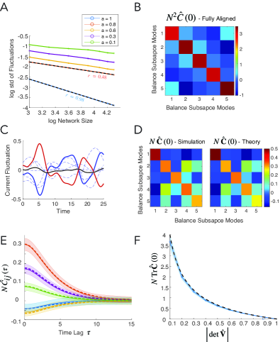
Figure 3: Partial Misalignment Can Increase Fluctuations in the Balance Subspace. (A) Log-log plot of total macroscopic temporal fluctuations vs network size, i.e. $\frac{1}{2}\log_{10}\underset{}{\mathrm{Tr}}\hat{\mathbf{C}}\left(0\right)$ vs $\log_{10}N$, for varying values of alignment parameter, $a$ ($a=1$ is fully aligned. See D1 - Constructing Arbitrary Low-Rank Structure with Uniform Misalignment for details). Linear fit (dashed line) shows that standard deviation of fluctuations scales as $\frac{1}{\sqrt{N}}$for networks with incomplete alignment, as compared to $\frac{1}{N}$ for fully aligned networks. (B) The $D$-by-$D$ covariance of firing rate fluctuaitons in the balance subspace, $\hat{\mathbf{C}}\left(0\right)$, for a fully aligned network is structureless. Compare (D) for case of incomplete alignment. (C) Sample trace of fluctuations in input currents onto a single mode of the balance subspace ($D=5$, $N=8000$ in this example). $O\left(1\right)$ fluctuations in the “effective-feedforward” input from the orthogonal subspace (red) are canceled by fluctuations in the “subspace-recurrent input” from within the balance subspace (blue, dotted line displays individual input modes and solid line displays net current fluctuations). Block solid line displays net flucutations in input current, which are $O\left(\frac{1}{\sqrt{N}}\right)$. (D) $D$-by-$D$ covariance of firing rate fluctuations in the balance subspace, displayed here scaled by $N$. (i.e. $N\hat{\mathbf{C}}\left(0\right)$). Left: single trial simulation. Right: Theory given by Eqn 11. (E) Time course of cross-correlation function between pairs of modes, scaled by $N$, $N\hat{C}_{ij}\left(\tau\right)$. Red is the autocorrelation, other colors display cross-correlation. Dotted lines show theory (Eqn 11). Solid lines show simulation results with shaded regions displaying standard deviation over 20 random realizations of $\mathbf{U}$ for fixed $\hat{\mathbf{V}}$. In (C) and (D), $\left|\det\hat{\mathbf{V}}\right|=0.2255$, the the singular values of $\hat{\mathbf{V}}$ were set to be $\left\{0.9,0.825,0.75,0.675,0.6\right\}$ (see Appendix Methods for more details). (F) Total variance of firing rate fluctuations in the balance subspace, scaled by $N$, plotted against the determinant of the alignment matrix, $\hat{\mathbf{V}}$. Blue shows simulation results with standard deviation over 20 random realizations. Dotted black line shows theory as given by Eqn 12. In these simulations, the external drive, $\mathbf{f}$, was rescaled in order to fix the norm of the balance firing rates, $\left\|\hat{r}^{*}\right\|$ (see Appendix Methods for more details) $N=10000$ in all simulations unless otherwise noted.

IV Biologically Relevant Examples

IV.1 Degenerate Excitation-Inhibition Balance

We first provide a sketch of the application of our generalized balance framework in the well-known setting of excitation-inhibition balance. Typically such a network is constructed by randomly and independently assigning connections to a fraction, $p$, of all pairs of neurons, with the synaptic weight (and sign) from neuron $j$ to neuron $i$ depending on each of their identities as either excitatory or inhibitory:

$$W_{ij}=\begin{cases}\pm\frac{J_{\alpha_{i}\alpha_{j}}}{p\sqrt{N}}&\mathrm{with\;\mathrm{prob\;}}p\\ 0&\mathrm{with}\;\mathrm{prob\;}1-p\end{cases}$$ (13)

where $\alpha_{i}=I$ for $N_{I}$ inhibitory neurons, and $\alpha_{i}=E$ for the remaining $N_{E}$ excitatory neurons, and the sign of the weight is corresponding to the pre-synaptic neuron, so that if $\alpha_{j}=E$ ($I$) the $j$th column of $W$ is positive (negative). Such a random binary connectivity matrix can be approximated by a low-rank, deterministic component with a $2$-by-$2$ block structure, and an additional random component (Kadmon and Sompolinsky, 2015). The low-rank component, though it is not symmetric because of the excitation-inhibition structure, is in general fully aligned: The balance subspace is the two-dimensional subspace spanned by two block-vectors, one with matching signs and one with opposing signs:

$$\mathbf{u}_{0}\sim\left(\begin{array}[]{c}+\\ +\end{array}\right)$$ (14)

$$\mathbf{u}_{1}\sim\left(\begin{array}[]{c}+\\ -\end{array}\right)$$ (15)

That is, the balance subspace consists of a “sum mode” and a “difference mode” of the excitatory and inhibitory populations. The read-out performed by the structured connectivity is from the same subspace, that is, the span of $\left\{\mathbf{v}_{0},\mathbf{v}_{1}\right\}$ is identical and therefore the alignment matrix is orthonormal.

However, consider the situation in which the synaptic weight is independent of the identity of the post-synaptic neuron: $J_{EI}=J_{II}=J_{I}$ and $J_{EE}=J_{IE}=J_{E}$. Because the average synaptic strengths in this network do not depend on the identity of the post-synaptic neuron, the structured component of connectivity is rank one: it is the outer product of a sum-mode and a difference mode. As Helias et al Helias et al. (2014) have also shown, this parameterization yields amplified fluctuations in both the E and I populations. We now show that this these fluctuations can be characterized as a specific case of our theory of incomplete alignment.

For simplicity, we assume $N_{I}=N_{E}=\frac{N}{2}$, (see Appendix G1 - Degenerate Excitation-Inhibition Balance Example for Unequal Population Size for general case). Explicitly we write the structured component of connectivity as $\frac{\sigma}{\sqrt{N}}\mathbf{u}_{0}\mathbf{v}_{0}^{T}$, according to our generalized balance formalism, with the following definitions:

$$\mathbf{u}_{0}=\left(\begin{array}[]{c}\mathbf{1}\\ \mathbf{1}\end{array}\right)$$ (16)

$$\mathbf{v}_{0}=\frac{1}{\sigma}\left(\begin{array}[]{c}J_{E}\mathbf{1}\\ -J_{I}\mathbf{1}\end{array}\right)$$ (17)

$$\sigma=\sqrt{\frac{J_{E}^{2}+J_{I}^{2}}{2}}$$ (18)

where $\mathbf{1}$ is the uniform column-vector of length $\frac{N}{2}$.

We observe that the alignment matrix is a scalar in this case, and is given by:

$$\hat{v}=\frac{1}{N}\mathbf{u}^{T}\mathbf{v}=\frac{J_{E}-J_{I}}{2\sigma}$$ (19)

Inhibition-dominance and network stability will require that $J_{I}\geq J_{E}$. We assume the external drive is uniform, $\mathbf{f}=\mathbf{1}r_{0}$, and then the balance equation yields population average firing

$$\hat{r}=-\frac{r_{0}}{\hat{v}\sigma}=\frac{2r_{0}}{J_{I}-J_{E}}$$ (20)

As the relative strength of inhibition decreases toward parity with excitation, the alignment between $\mathbf{v}_{0}$ and $\mathbf{u}_{0}$ shrinks: the row-vector, $\mathbf{v}_{0}^{T}$, reads out the difference between net E and I activity, while the column-vector, $\mathbf{u}_{0}$, drives E and I equally. To avoid saturation while changing the I-E ratio, the external drive must shrink to compensate for diminished alignment, by scaling $r_{0}\propto\hat{v}\sigma=J_{I}-J_{E}$.

Applying our theory (Eqn 11) we find that reduced I-E ratio will lead to larger fluctuations of the population firing rate, $\hat{C}\left(\tau\right)=\left\langle\hat{r}\left(t\right)\hat{r}^{T}\left(t+\tau\right)\right\rangle$:

$$\hat{C}\left(\tau\right)=\frac{C\left(\tau\right)}{N}\left(\frac{J_{E}+J_{I}}{J_{E}-J_{I}}\right)^{2}$$ (21)

By fixing $J_{E}$ and varying the ratio $\frac{J_{I}}{J_{E}}$ while scaling $r_{0}$ to maintain the balance firing rate, we confirm this prediction via simulations in Figure 4F.

Note that in the limit of $J_{I}\rightarrow J_{E}$, the expression for the size of these fluctuations diverges. In that limit, external drive must be zero in order to avoid saturation, and the size of the fluctutaions along $\mathbf{u}_{0}$, i.e. coherent fluctuations shared by the entire population, is $O\left(1\right)$. Our theory breaks down once the fluctuations in $\hat{r}$ are sufficiently large relative to $\frac{1}{\sqrt{N}}$, as they begin to significantly impact the fluctuations in the orthogonal complement (Landau and Sompolinsky, 2018; Hayakawa and Fukai, 2020).

IV.2 Heterogeneous Out-Degrees

We now employ our theory of misalignment to study the dynamics of networks with heterogeneous out-degrees (see Appendix G2 - Heterogeneous In- and Out-Degrees for the case of both heterogeneous out- and in-degrees). Consider a single inhibitory population in which each neuron $i$ has $K_{i}$ randomly chosen outgoing connections, with each non-zero synapse having weight $-\frac{J}{\sqrt{N}}$, where $K$ is the average number of connections per neuron. Just as in the E-I setting, such a random binary connectivity structure can be approximated by a deterministic low-rank component and a random component of connectivity. The deterministic component in this case can be written as:

$$M_{ij}=\frac{J}{\sqrt{N}}\frac{k_{j}}{N}$$ (22)

where we have defined the relative out-degrees, $k_{i}\equiv\frac{K_{i}}{K}$.

This deterministic $\mathbf{M}$ is a rank-one matrix given by $\mathbf{M}=\sigma\mathbf{u}_{0}\mathbf{v}_{0}^{T}$, with the following definitions:

$$\mathbf{u}=\mathbf{1}$$ (23)

$$\mathbf{v}=\frac{\mathbf{k}}{\sqrt{\left\langle k^{2}\right\rangle}}$$ (24)

$$\sigma=\sqrt{\left\langle k^{2}\right\rangle}Jp$$ (25)

where $p\equiv\frac{K}{N}$, $\left\langle k^{2}\right\rangle$ is the mean-square of the relative out-degrees, and $\mathbf{1}$ is the column vector of all ones.

The alignment matrix is scalar in this case as well and is given by

$$\hat{v}=\frac{\mathbf{1}^{T}\mathbf{k}}{N}\frac{1}{\sqrt{\left\langle k^{2}\right\rangle}}=\frac{1}{\sqrt{\left\langle k^{2}\right\rangle}}$$ (26)

Thus we see that the extent of alignment, and therefore the strength of “subspace reccurence” decreases with increasing breadth of the out-degree distributions

The balance equation gives

$$\hat{r}=-\frac{r_{0}}{\hat{v}\sigma}=\frac{r_{0}}{Jp}$$ (27)

such that the balance firing rates in the population are unaffected by broadening of the out-degree. This is intuitive because the mean recurrent input is not expected to depend on the breadth of the out-degree.

Nevertheless, broad a out-degree distribution increases the extent of coherent fluctuations, as decreased alignment means an increasing of “effective-feedforward” connectivity from the orthogonal complement to the balance subspace. Concretely, we have:

$$\hat{C}\left(\tau\right)=\frac{C\left(\tau\right)}{N}\left(\left\langle k^{2}\right\rangle-1\right)$$ (28)

Note that $\left\langle k^{2}\right\rangle-1$ is exactly the variance of the relative out-degrees. The increase of correlations with broader out-degree was observed in Roxin (2011).

We find that broader out-degree distribution leads to larger coherent fluctuations and confirm this prediction via simulations (Fig 4F). It is worth noting that the structure of $\mathbf{V}_{\perp}$ does not enter the mean-field theory, beyond the assumption that $\boldsymbol{\eta}=\frac{1}{\sqrt{N}}\mathbf{V}_{\perp}^{T}\delta\mathbf{r}$ is an independent mean-zero Gaussian process. In practice, we generate out-degrees from a log-normal distribution and find that the simulations fit the theory well within a broad range of out-degree variability, although the fit worsens as the variability increases, as presumably the Gaussian assumption is violated.

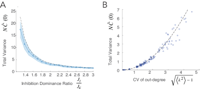
Figure 4: Biologically Relevant Examples of Incomplete Alignment Yiedling Low-Dimensional Fluctuations (A) E-I network with degenerate weight parameters in the sense that the strength of both E and I synapses are independent of the identity of the post-synaptic neuron. Variance of population firing rate over time, scaled by $N=20000$ in this simulation. Dotted black line shows theory (Eqn 21). Shaded region shows standard error of the mean over 20 trials. (B) Inhibitory network with heterogeneous out-degree. Variance of the population firing rate over time, scaled by $N$, as a function of the coefficient of variation (CV) of the the out-degree. Dotted line shows theory (Eqn 28). Circles show single trial simulations. Out-degrees were drawn from a log-normal distribution. In-degrees were taken to be uniform. $N=10000$.

V Discussion

We have generalized the theory of dynamic excitation-inhibition balance to networks with arbitrary low-rank structured connectivity, $\mathbf{M}=\frac{1}{\sqrt{N}}\mathbf{U}\boldsymbol{\Sigma}\mathbf{V}^{T}$, together with an additive random component of connectivity. We decompose the network dynamics into the “balance subspace”, given by $\mathrm{span}\left(\mathbf{U}\right)$, which receives strong structured recurrent input, and its orthogonal complement within which the recurrent input is driven by random connectivity. The core insight of our theory is that the macroscopic, low-dimensional dynamics in the balance subspace are determined by the alignment matrix, $\hat{\mathbf{V}}=\frac{1}{N}\mathbf{U}^{T}\mathbf{V}$, between left- and right-singular vectors. We derive linear balance equations for the activity in the balance subspace which are a generalization of the two balance equation in excitation-inhibition networks. These balance equations are independent of the underlying statistics of the balance subspace itself, $\mathbf{U}$, but rather depend only on the alignment, $\hat{\mathbf{V}}$, and the singular values, $\boldsymbol{\Sigma}$, which scale the recurrent connectivity in each of the balance subspace modes.

We observe that $\hat{\mathbf{V}}$quantifies the alignment between row-space and column-space of the structured connectivity, that is, between the the read-out and feed-back subspaces. If the read-out subspace is identical to the feed-back subspace, then $\hat{\mathbf{V}}$ is orthonormal. If $\hat{\mathbf{V}}$ is not an orthonormal matrix then the structured connectivity is not fully aligned. In this case the structured connectivity can be decomposed to a subspace-recurrent component that reads-out network activity strictly from within the balance subspace, and an effective-feedforward component that reads-out network activity from the orthogonal complement and projects it to the balance subspace.

We show that increased misalignment increases coherent, low-dimensional fluctuations in the balance subspace. This is due to the strengthening of the effective-feedforward component of the structured connectivity, which reads-out microscopic fluctuations from the orthogonal complement and projects them to the balance subspace. It is important to emphasize that the fluctuating input currents projected from the orthogonal complement to the balance subspace are of $O\left(1\right)$, but that balance leads to a dynamic canceling of these fluctuating currents to leading order. This cancelation is manifested by a set of fluctuation-balance equations that enable us to determine the size, structure, and temporal profile of firing rate fluctuations in the balance subspace, $\hat{\mathbf{C}}\left(\tau\right)$, as a function of $\hat{\mathbf{V}}$. Despite the suppression of fluctuations via dynamic balance, the magnitude of coherent fluctuations due to misalignment is an order of magnitude larger than under fully aligned connectivity. These fluctuations increase with misalignment as a function of the singular values of $\hat{\mathbf{V}}$, as the subspace-recurrent feedback is weakened requiring larger macroscopic fluctuations in order to cancel the input fluctuations from the orthogonal complement. Because they are driven by the microscopic fluctuations in the orthogonal complement, the temporal profile of these shared macroscopic fluctuations is identical to the average temporal profile of single-neuron fluctuations. The spatial structure of the fluctuations within the $D$-dimensional balance subspace is given by the left-singular vectors of the alignment matrix.

Note that in the limit where at least one of the singular values of $\hat{\mathbf{V}}$ is zero, fluctuation balance cannot be achieved along the corresponding modes. Any external drive into these modes will drive saturation, but if there is no external drive to these modes, then the fluctuations in the orthogonal complement will be propagated to this mode via the structured connectivity in a fully feed-forward manner, without being suppressed by dynamic balance. This can lead to $O\left(1\right)$ shared fluctuations as studied in (Landau and Sompolinsky, 2018).

We have studied continuous rate-neuron models, for their analytical tractability. However, we expect that our theory will hold qualitatively for spiking-neuron network models as well. This is because we find that despite the elevated shared fluctuations, networks with incomplete alignment exhibit asynchronous dynamics as long as the singular values of $\hat{\mathbf{V}}$are non-zero. Thus we expect that spiking networks with strong low-rank connectivity structure will operate in an asynchronous, irregular regime that is well-described by a mean-field theory (Brunel, 2000) which can be etended to include the impact of misaligned structure as we have done here.

We have studied the structure of temporal fluctuations but our approach can be readily extended to study the structure of quenched variability over multiple realizations of the random connectivity. We expect that incomplete alignment will amplify quenched fluctuations in a similar manner.

Note that throughout this work we assume that the external drive vector, $\mathbf{\hat{\mathbf{f}}}$, is such that enables a balanced fixed point. This requires that the external drive be almost entirely contained in the balance subspace (up to $O\left(\frac{1}{\sqrt{N}}\right)$ projections). The impact of misaligned external drive is to effectively weaken the input to the balance subspace, thus shifting the balance fixed point and eventually suppressing chaos and yielding saturation, as we showed in (Landau, 2020). In addition, a balanced fixed points imposes further constrains on $\hat{\mathbf{f}}$. For example, in standard E-I balance networks, external drive onto the E population must be sufficiently stronger that that onto the I population in order to maintain non-negative firing rates (van Vreeswijk and Sompolinsky, 1998; Baker et al., 2020). Describing these constraints in the general low-rank setting is beyond the scope of this work.

We note that the random component of connectivity may have statistical structure, for example different cell-types may have different overall variability of their synaptic strengths yielding a block-structure on the variances (Aljadeff et al., 2015; Kadmon and Sompolinsky, 2015; Schuessler et al., 2020). Additionally, the low-rank structure may be correlated with the random component of connectivity (Schuessler et al., 2020). These types of correlations in the connectivity may have non-trivial impact in the regime of dynamic balance which may be of interest for future study.

Relationship to Previous Models of Dynamic Balance

Our framework of generalized dynamic balance unifies much previous work. For example the typical E-I balance network has rank-$2$ deterministic structure, in which both the column-space and row-space consist of a “sum” mode and a “difference” mode, and therefore the structure is fully aligned. Some E-I network models (e.g. (Brunel, 2000; Ostojic, 2014)), however, use a degenerate block-structure by constraining the average weights to be independent of post-synaptic population. As we have shown here, in this case, the structured connectivity has rank $1$ and is only partially aligned. The balance subspace is a sum mode, $\mathbf{u}_{0}\propto\mathbf{1}$, while the read-out mode, $\mathbf{v}_{0}$, is a difference mode. As the relative strength of inhibition decreases, the recurrent connectivity becomes less alignedand yields larger and larger coherent fluctuations. These increased fluctuations in the case of degenerate E-I structure have been previously studied in (Helias et al., 2014). As suggested in the discussion in (Helias et al., 2014), even stronger correlations arrise in the case of a “doubly-degenerate” E-I structure, in which in addition to being independent of post-synaptic population, the average weights are set to zero. Such a case was studied in (Hayakawa and Fukai, 2020) and corresponds to the limit where $\hat{\mathbf{V}}=0$ in our formalism.

E-I networks with distance dependent connectivity have been the focus of a number of past studies (van Vreeswijk and Sompolinsky, 2005; Rosenbaum and Doiron, 2014; Darshan et al., 2018; Ebsch and Rosenbaum, 2020). In the typically studied setting, each of the E and I connectivity profiles share the same periodic boundary conditions and are constrained to finite spatial frequency modes, and therefore both the column-space and row-space are spanned by a concatenated Fourier basis of E and I cells, and therefore$\hat{\mathbf{V}}$ is orthonormal. (Darshan et al., 2018) present cases in which E-I networks with distance-dependent connectivity have a singular $\hat{\mathbf{V}}$. For example, they consider the case in which the I-to-E connectivity has spatial dependence while all other connectivity profiles are spatially uniform. In our formalism, the column-space (columns of $\mathbf{U}$) no longer includes Fourier modes of the I population, but rather consists of Fourier modes of the E population concatenated with the zero vector over the I population. On the other hand the row-space (columns of $\mathbf{V})$ does not include Fourier modes from the E population, but rather, consists of I-population Fourier modes concatenated with the zero vector over the E population, and these modes are entirely orthogonal to $\mathbf{U}$ so that they are fully feed-forward. Thus spatially correlated fluctuations are propagated from the I population to the E population, where they are not canceled. As further discussed in (Darshan et al., 2018), the situation is different if the I population has distant-dependent connectivity internally as well. In our formalism this would mean that while columns of $\mathbf{V}$ would still not include Fourier modes of E, the columns of $\mathbf{U}$ would once again consist of the concatenated E and I Fourier modes. Thus, this is an example of partial alignment. Therefore, the spatially correlated fluctuations in the presence of I-to-I distance dependent are an order of magnitude smaller than the purely feed-forward case, they are still an order of magnitude larger than in the fully aligned case in which the E population also has distance-dependent projections (whether to itself or to the I population).

Networks with heterogeneous in-degrees have been previously shown to exhibit broken balance (Pyle and Rosenbaum, 2016; Landau et al., 2016). That result can be undestood in a straightforward manner in our framework of generalized balance: if the in-degrees from the external drive are not a linear combination of E and I in-degrees, then the external drive is not fully aligned with the balance subspace and there will be strong external drive to the orthogonal complement which will drive saturation (Landau, 2020). In addition to heterogeneous in-degrees, here we have studied the impact of heterogeneous out-degrees on dynamic balance. We show that broad out-degree distributions in balanced networks are a form of incomplete alignment and result in increased coherent fluctuations. A similar phenomenon was observed numerically in (Roxin, 2011). We provide an analytical expression for the size of fluctuations as a function of the breadth of the out-degrees, and verify it numerically. We furthermore show that negative correlations between in- and out-degrees will further amplify the shared fluctuations (AppendixG2 - Heterogeneous In- and Out-Degrees)

Other work has shown that balance networks can exhibit shared variability if they have shared fluctuations in their external input (Darshan et al., 2017; Rosenbaum et al., 2016). Our work assumes a constant external input.

Conclusion

Previous studies have explored particular examples of low-rank deterministic structure in balanced networks, most often via distance-dependent connectivity (van Vreeswijk and Sompolinsky, 2005; Rosenbaum and Doiron, 2014; Rosenbaum et al., 2016; Darshan et al., 2018) or sub-population structure (Kadmon and Sompolinsky, 2015; Darshan et al., 2017). In such low-rank structures, the column-space (the span of the left-singular vectors) is typically identical to the row-space (the span of the right-singular vectors). We call such networks “fully aligned”, and study the more general situation of partial alignment in which the row-space is not entirely contained in the column-space of the low-rank matrix. We show that such incomplete alignment can have qualitative impact on network dynamics. The key feature of the structured connectivity in our analysis is the alignment matrix, comprised of the overlaps between left- and right-singular vectors.

Low-rank structured connectivity may reflect different cell-types, distance-dependence, functional connectivity, as well as heterogeneity between neurons (van Vreeswijk and Sompolinsky, 2005; Rosenbaum and Doiron, 2014; Landau et al., 2016; Darshan et al., 2018). Such a generalization may be important for incorporating biological realism into balance-network models. From another perspective, low-rank structure has been of recent interest in designing networks that perform specific computations (Sussillo and Abbott, 2009; Mastrogiuseppe and Ostojic, 2018). Our work studies a new regime where low-rank connectivity is strong, and suggests a bridge between networks designed for computation and biological networks exhibiting dynamic balance.

We have developed a generalized theory of dynamic balance, which both unifies previous studes and reveals new results. Our generalization expands the study of dynamic balance to a broad class of low-rank structures – those with only partial alignment between column-space and row-space. These structures have previously only appeared in particular cases, but in our framework they appear as the general case of low-rank connectivity. We show that incomplete alignment generates coherent fluctuations via effective-feed-forward propagation from a high-dimensional subspace with microscopic chaos to a low-dimensional, balance subspace. We derive a set of fluctuation balance equations that provides an analytical solution for the structure of coherent fluctuations in the balance subspace.

This theory may find relevance well beyond neuroscience. Recent studies of complex systems attempt to explore the relationship between structure and dynamics in a variety of real-world networks (Barzel and Barabási, 2013; Hens et al., 2019). Many of these studies limit the strength of interaction between units ($\sim\frac{1}{N}$) in order to facilitate mean-field approaches. The theory of excitation-inhibition balance studies a regime of strong interactions ($\sim\frac{1}{\sqrt{N}}$) but until now its application has remained limited to neuroscience because of the excitation-inhibition structure (Dale’s Law). Our generalized framework of dynamic balance may be relevant for any setting with strongly interacting units, whether biological, social, or technological networks.

Appendix

Appendix A - Self-Consistency of the Balance Solution

As discussed in the bain text, the macroscopic dynamics in the balanced subspace (Eqn 5) admit a balanced fixed point governed by the $D$ linear balance equations: $\boldsymbol{\Sigma}\hat{\mathbf{V}}^{T}\hat{\mathbf{r}}^{*}+\hat{\mathbf{f}}\approx 0$ (Eqn 6 in the main text). Balance is achieved when the firing rates in the balance subspace satisfy this equation up to a finite-size correction of $\frac{1}{\sqrt{N}}$. These firing rates, $\hat{\mathbf{r}}$, are given by the components of the full population firing rate vector, $\mathbf{r}=\phi\left(\mathbf{h}\right)$, along $\mathbf{U}$:

$$\hat{\mathbf{r}}^{*}=\frac{1}{N}\mathbf{U}^{T}\phi\left(\mathbf{U}\hat{\mathbf{h}}^{*}+\mathbf{h}_{\perp}\right)$$ (29)

As we shall see, these $D$ equations constrain both the residual fields in the balance subspace, $\hat{\mathbf{h}}^{*}$ , as well as the statistics of the microscopic, local dynamics in the orthogonal complement, $\mathbf{h}_{\perp}$.

The dynamical state in the orthogonal complement can be either a stable fixed point (FP) or chaos. Given a fixed $\hat{\mathbf{h}}^{*}$, those dynamics are described by a mean-field theory that predicts that the microscopic degrees of freedom, $h_{\perp_{i}}$, are be described as independent, identical, mean-zero Gaussians, either fixed in time or fluctuating with a monotonically decaying autocorrelation. The mean-field theory follows previous work (e.g. (Sompolinsky et al., 1988; Kadmon and Sompolinsky, 2015)), and we detail it for our setting below in Appendix Appendix B - Mean-Field Theory in the Orthogonal Subspace. The result of the mean-field theory is that if balance is achieved, avoiding saturation, then there is a FP with Gaussian statistics that transitions to chaos for sufficiently strong random component of connectivity. The expression for the variance in the orthogonal subspace, $\Delta_{0}=\left\langle h_{\perp_{i}}^{2}\right\rangle$, depends only on $\hat{\mathbf{h}}^{*}$ and $g$. In the FP regime, $\Delta_{0}$ is the spatial disorder and is given by a single implicit equation, while in the chaotic regime, $\Delta_{0}$ averages both spatial and temporal disorder and is constrained by a pair of equations together with the spatial variance of the single-neuron long-time averages.

Given, $\Delta_{0}$, $\hat{\mathbf{r}}$ is given by first averaging over the Gaussian component in the orthogonal subspace and then projecting the result onto balance subspace:

$$\hat{\mathbf{r}}^{*}=\frac{1}{N}\mathbf{U}^{T}\left\langle\phi\left(\mathbf{U}\hat{\mathbf{h}}^{*}+\sqrt{\Delta_{0}}z\right)\right\rangle_{Dz}$$ (30)

where $\left\langle\right\rangle_{Dz}$ is an integral over the standard normal measure, $Dz=\frac{dz}{2\pi}\mathrm{\mathrm{e}}^{-\frac{z^{2}}{2}}$. Combining the balance balance requirement $\hat{\mathbf{r}}^{*}\approx\hat{\mathbf{r}}^{bal}$ (Eqn 6) gives us a set of $D$ implicit equations, which given $\Delta_{0}$, determine $\hat{\mathbf{h}}^{*}$:

$$\frac{1}{N}\mathbf{U}^{T}\left\langle\phi\left(\mathbf{U}\hat{\mathbf{h}}^{*}+\sqrt{\Delta_{0}}z\right)\right\rangle_{Dz}=-\hat{\mathbf{V}}\boldsymbol{\Sigma}^{-1}\hat{\mathbf{f}}$$ (31)

We stress that this Gaussian mean-field equation for self-consistency in the balance subspace holds regardless of whether the dynamics in the orthogonal subspace are in the FP or chaotic regime, but the total variance in the orthogonal subspace, $\Delta_{0}$, must also be found in a manner self-consistent with $\hat{\mathbf{h}}^{*},$as we show below.

Appendix B - Mean-Field Theory in the Orthogonal Subspace

We now detail the mean-field theory describing the dynamics in the orthogonal subspace for both fixed point and chaos. We will assume an approximate fixed point in the balance subspace, $\hat{\mathbf{h}}^{*}$, that enables the corresponding firing rates, $\hat{\mathbf{r}}^{*}$, to satisfy the $D$ balance equations (Eqn 6).

We further assume full external alignment, as we have throughout the main text, so that the external drive, $\mathbf{f}$, does not project into the orthogonal subspace. The dynamics are given by:

$$\dfrac{\mathrm{d}\mathbf{h}_{\perp}}{\mathrm{d}t}=-\mathbf{h}_{\perp}+\frac{g}{\sqrt{N}}\mathbf{J}_{\perp}\mathbf{r}$$ (32)

where, we remind the reader, $\mathbf{X}_{\perp}=\left(\mathbf{I}-\frac{1}{N}\mathbf{U}\mathbf{U}^{T}\right)\mathbf{X}$ is the orthogonal compliment of the vector or matrix of column-vectors, $\mathbf{X}$, and the vector of firing rates is given by $\mathbf{r}=\phi\left(\mathbf{h}\right)$. Through the non-linearity, $\phi$, the dynamics in the orthogonal complement depend on the dynamics in the balance subspace, $\hat{\mathbf{h}}^{*}$.

B1 Fixed Point and its Stability

The fixed point equation in the orthogonal subspace is

$$\mathbf{h}_{\perp}^{*}=\mathbf{J}_{\perp}\mathbf{r}^{*}$$ (33)

Given a fixed $\hat{\mathbf{h}}^{*}$, we follow the mean-field theory presented, for example in (Kadmon and Sompolinsky, 2015), which treats the recurrent drive due to the random connectivity, as independent, identical, mean-zero Gaussians. This theory assumes that due to the random connectivity, $\left(\sum_{j}^{N}J_{\perp_{ij}}r_{j}\right)^{2}\approx\sum_{j}J_{\perp_{ij}}^{2}r_{j}^{2}\approx N\left\langle J_{ij}^{2}\right\rangle\left\langle r_{j}^{2}\right\rangle$, which therefore determines the spatial variance at the fixed point, $\Delta_{0}\equiv\left\langle h_{\perp_{i}}^{2}\right\rangle$, to be

$$\Delta_{0}=g^{2}\left\langle r_{j}^{2}\right\rangle$$ (34)

The mean-square firing rates, $\left\langle r_{j}^{2}\right\rangle=\left\langle\phi^{2}\left(h_{j}\right)\right\rangle$, must be found by averaging over the network, where $h_{j}$ has a component in the balance subspace and an additional Gaussian component with variance $\Delta_{0}$. Because the two components are independent, we can perform the average over the Gaussian randomness before averaging over the population, and thus we arrive at an implicit mean-field fixed-point equation for $\Delta_{0}$:

$$\Delta_{0}=g^{2}\frac{\mathbf{1}^{T}}{N}\left\langle\phi^{2}\left(\mathbf{U}\hat{\mathbf{h}}^{*}+\sqrt{\Delta_{0}}z\right)\right\rangle_{Dz}$$ (35)

where $\left\langle\right\rangle_{Dz}$ means averaging over the standard normal measure $Dz=\mathrm{e}^{-\frac{z^{2}}{2}}dz$.

Given a fixed $\hat{\mathbf{h}}^{*}$, the Jacobian matrix for the stability of the fixed point in the orthogonal complement is given by $J_{\perp_{ij}}\phi^{\prime}\left(h_{j}\right)$. As we have done previously, we assume that $h_{j}$ is independent of $J_{\perp_{ij}}$, and this Jacobian matrix is a random matrix with column-wise variance. The support of the eigenvalues of such a matrix is identical that of a random matrix with uniform variance that is given by the average of the column-wise variances (Ahmadian et al., 2015). Thus, the effective gain at the fixed point, which is given by the maximal real part of the eigenvalues of the Jacobian, is given by $g_{eff}^{2}=\left\langle J_{\perp_{ij}}^{2}\right\rangle\left\langle\phi^{\prime}\left(h_{j}\right)^{2}\right\rangle$, which can be calculated as:

$$g_{eff}^{2}=g^{2}\frac{\mathbf{1}^{T}}{N}\left\langle\phi^{\prime 2}\left(\mathbf{U}\hat{\mathbf{h}}^{*}+\sqrt{\Delta_{0}}z\right)\right\rangle_{Dz}$$ (36)

The fixed point in the orthogonal complement, $\mathbf{h}_{\perp}^{*}$, will be stable for $g_{eff}<1$, and for $g_{eff}>1$ the microscopic dynamics in the orthogonal compliment will be chaotic. Those dynamcis are described by a dynamic mean-field theory (DMFT), detailed in the next section.

The stability calculation here is equivalent to considering perturbations within the orthogonal complement, with the balance subspace held fixe. A complete treatment of stability should consider arbitrary perturbations, in both the orthogonal complement and the balance subspace, following (Kadmon and Sompolinsky, 2015; Mastrogiuseppe and Ostojic, 2018).

B2 - Dynamic Mean-Field Theory of Chaos in the Orthogonal Subspace

In the chaotic regime, the input to the orthogonal subspace can still be considered Gaussian but its temporal statistics must be derived, that is we seek to find the autocorrelation:

$$\Delta\left(\tau\right)\equiv\left\langle h_{i}^{\perp}\left(t\right)h_{i}^{\perp}\left(t+\tau\right)\right\rangle$$ (37)

The dynamics in the orthogonal subspace can be represented by a single stochastic differential equaiton:

$$\dfrac{\mathrm{d}h_{i}^{\perp}}{\mathrm{d}t}=-h_{i}^{\perp}+\eta_{i}$$ (38)

where $\eta_{i}\left(t\right)=\sum_{j}J_{ij}^{\perp}r_{j}\left(t\right)$. Again, due to the randomness of the connectivity, $\eta_{i}$ has mean-zero over neurons and time, and the average autocorrelation of $\eta_{i}$ is a scaled version of the average autocorrelation of $r_{i}$:

$$\left\langle\eta_{i}\left(t\right)\eta_{i}\left(t+\tau\right)\right\rangle=g^{2}C_{T}\left(\tau\right)$$ (39)

where we have written

$$C_{T}\left(\tau\right)\equiv\left\langle\phi\left(h_{i}\left(t\right)\right)\phi\left(h_{i}\left(t+\tau\right)\right)\right\rangle$$ (40)

for the average autocorrelation of the firing rates. Note that the notation $\left\langle\;\right\rangle$ now denotes averaging over both time and neurons. Additionally, note that we have inserted the notation $C_{T}$ for the total autocorrelation in order to differentiate from the mean single-neuron temporal autocorrelation ($C\left(\tau\right)=C_{T}\left(\tau\right)-\left\langle\phi\left(h_{i}\right)\right\rangle^{2}$) introduced in the main text in Section III, Equation 11.

To compute $C_{T}\left(\tau\right)$ we first write $h_{i}=\mathbf{u}_{i}^{T}\hat{\mathbf{h}}^{*}+h_{i}^{\perp}$, where $\mathbf{u}_{i}$ is the $i$th row of the left-singular vector matrix, and gives the projection of neuron $i$ in the balance subspace. Next we rewrite the two correlated Gaussians, $h_{i}^{\perp}\left(t\right)$ and $h_{i}^{\perp}\left(t+\tau\right)$, via three independent Gaussians, one of which contributes the correlated component:

$$h_{i}^{\text{$\perp$}}\left(t\right)=\sqrt{\Delta_{0}-\Delta\left(\tau\right)}x_{1}+\sqrt{\Delta\left(\tau\right)}y$$ (41)

$$h_{i}^{\perp}\left(t+\tau\right)=\sqrt{\Delta_{0}-\Delta\left(\tau\right)}x_{2}+\sqrt{\Delta\left(\tau\right)}y$$ (42)

where we have introduced $\Delta_{0}\equiv\Delta\left(0\right)$ as the total variance. These three Gaussians need to be integrated over, and then the balance subspace structure averaged to yield

$$C_{T}\left(\tau\right)=\frac{1}{N}\sum_{i}\left\langle\left\langle\phi\left(\mathbf{u}_{i}^{T}\hat{\mathbf{h}}^{*}+\sqrt{\Delta_{0}-\Delta\left(\tau\right)}x+\sqrt{\Delta\left(\tau\right)}y\right)\right\rangle_{Dx}^{2}\right\rangle_{Dy}$$ (43)

Thus given the autocorrelation, $\Delta\left(\tau\right)$, in the orthogonal complement, we have an expression for the average single neuron firing rate autocorrelation, $C_{T}\left(\tau\right)$. Next, following the standard DMFT approach ((Sompolinsky et al., 1988; Kadmon and Sompolinsky, 2015)) we write an implicit differential equation that determines the autocorrelation self-consistently:

$$\left(1-\dfrac{\partial^{2}}{\partial\tau^{2}}\right)\Delta\left(\tau\right)=g^{2}C_{T}\left(\tau\right)$$ (44)

The total variance, $\Delta_{0}$, is the initial condition of Eqn 44 and must be found self-consistently along with the conditions $\dfrac{\partial}{\partial\tau}\Delta\left(0\right)=0$ and $\dfrac{\partial^{2}}{\partial\tau^{2}}\Delta\left(\infty\right)=0$. As detailed in (Sompolinsky et al., 1988; Kadmon and Sompolinsky, 2015), the differential equation (Eqn 44) can be re-expressed as a one-dimensional dynamics under a potential energy. Given $\hat{\mathbf{h}}$, the initial condition, $\Delta_{0}$, can be found by using the requirement that the potential energy at the initial condition equals its value at $\tau\rightarrow\infty$, together with the fact that $\Delta\left(\infty\right)=g^{2}C_{T}\left(\infty\right)$. Therefore, in practice, given the fixed point in the balance subspace, $\hat{\mathbf{h}}^{*}$, the total variance in the orthogonal subspace, $\Delta_{0}=\left\langle\left(h_{i}^{\perp}\right)^{2}\right\rangle$, and the spatial variance of the time-averages, $\Delta\left(\infty\right)=\frac{1}{N}\sum_{i}\left\langle h_{i}^{\perp}\right\rangle_{t}^{2}$, are found via a pair of coupled equations. The fixed point in the balance subspace depends on $\Delta_{0}$ in turn, via the balance equations (Eqn 31).

In sum, the mean-field characterization of the system determines $\hat{\mathbf{h}}^{*}$ and $\Delta_{0}$ via either $D+1$ equations (in the FP regime) or $D+2$ equations (in the chaotic regime). When these equations are satisfied the network generalizes the dynamic balance of excitation-inhibition. This balance is dynamic in the sense that without fine-tuning, the macroscopic firing rates in the balance subspace self-adjust to cancel the strong external drive. Depending on the single-neuron transfer function and the strength of the random component of connectivity, balance can take the form of either a stable fixed-point, or the more familiar balanced state of chaotic dynamics with local fluctuations propagating in the orthogonal complement.

Appendix C - The Case of Gaussian Structured Connectivity

Here we study the mean-field theory for the case in which the structured connectivity is Gaussian. In particular, the elements of $\mathbf{U}$ are taken to be i.i.d. by $\mathcal{N}\left(0,1\right)$. The Gaussianity construction greatly simplifies the mean-field expression for $\hat{r}_{k}$ (Eqn 30). In the general case, calculating $\hat{r}_{k}$ requires first averaging $r_{i}=\phi\left(\mathbf{u}_{i}^{T}\hat{\mathbf{h}}+h_{i}^{\perp}\right)$ over the variability in the orthogonal subspace by a Gaussian integral for each neuron $i$ (where $\mathbf{u}_{i}$ is the $i$th row of $\mathbf{U}$ as above), and then computing a weighted average over the structure of the $k$th column of $\mathbf{U}$. That is

$$\hat{r}_{k}=\frac{1}{N}\sum_{i=1}^{N}u_{ik}\left\langle\phi\left(\sum_{l=1}^{D}u_{il}\hat{h}_{l}+\sqrt{\Delta_{0}}z\right)\right\rangle_{Dz}$$ (45)

In the Gaussian case, the other modes $l\neq k$ contribute Gaussian variablilty which can simply be added to the variability from the orthogonal subspace, and then $u_{ik}$ can be averaged over as an additional Gaussian. Therefore $\hat{r}_{k}$ reduces to a double Gaussian integral: one integral for the weighted average over the structure of the $k$th mode, which is coupled to $\hat{h}_{k}$, and a second Gaussian that combines the remaining $D-1$ structured modes together with the orthogonal complement:

$$\hat{r}_{k}=\left\langle u\,\phi\left(u\hat{h}_{k}+\sqrt{\Delta_{0}+\sum_{l\neq k}\hat{h}_{l}^{2}}z\right)\right\rangle_{DuDz}$$ (46)

The Gaussian integral over $u$ can be performed via integration by parts. Explicitly, one writes $w\equiv\mathrm{e}^{-\frac{u^{2}}{2}}u$ and $dv\equiv\phi\,du$, then $\int dv\,w=-\int dw\,v=\int Du\,\dfrac{\partial\phi}{\partial u}$. Now the two Gaussians, $u$ and $z$, combine to a single Gaussian integral:

$$\hat{r}_{k}=\hat{h_{k}}\left\langle\phi^{\prime}\left(\sqrt{\Delta_{0}+\left\|\hat{\mathbf{h}}\right\|^{2}}x\right)\right\rangle_{Dx}$$ (47)

We find that due to the Gaussianity of $\mathbf{U}$, $\hat{\mathbf{h}}$ is proportional to $\hat{\mathbf{r}}$. Therefore the $D$ equations for $\hat{h}_{k}$reduce to one implicit scalar equation for $\left\|\hat{\mathbf{h}}\right\|$:

$$\left\|\hat{\mathbf{r}}\right\|=\left\|\hat{\mathbf{h}}\right\|\left\langle\phi^{\prime}\left(\sqrt{\Delta_{0}+\left\|\hat{\mathbf{h}}\right\|^{2}}x\right)\right\rangle_{Dx}$$ (48)

where, of course, $\mathbf{\hat{\mathbf{r}}}$ is determined to leading order by the balance equations.

The Gaussianity of $\mathbf{U}$ also simplifies the mean-field calculation of the variance in the orthogonal complement, $\Delta_{0}$. In the FP equation (Eqn 35) the sum over neurons can be replaced by a Gaussian integral over the balance subspace and combined with the Gaussian integral over the orthogonal complement to yield

$$\Delta_{0}=g^{2}\left\langle\phi^{2}\left(\sqrt{\Delta_{0}+\left\|\hat{\mathbf{h}}\right\|^{2}}x\right)\right\rangle_{Dx}$$ (49)

Similarly, the effective gain at the FP in the orthogonal complement is given by

$$g_{eff}^{2}=g^{2}\left\langle\phi^{\prime 2}\left(\sqrt{\Delta_{0}+\left\|\hat{\mathbf{h}}\right\|^{2}}z\right)\right\rangle_{Dz}$$ (50)

Furthermore, we can simplify the dynamic mean-field expression for the total autocorrelation , $C_{T}\left(\tau\right)\equiv\left\langle\phi\left(h_{i}\left(t\right)\right)\phi\left(h_{i}\left(t+\tau\right)\right)\right\rangle$, as well. In Eqn 43:

$$C_{T}\left(\tau\right)=\left\langle\left\langle\phi\left(\sqrt{\Delta_{0}-\Delta\left(\tau\right)}x+\sqrt{\Delta\left(\tau\right)+\left\|\hat{\mathbf{h}}\right\|^{2}}y\right)\right\rangle_{Dx}^{2}\right\rangle_{Dy}$$ (51)

Thus we find that in the Gaussian setting, the DMFT calculation of the autocorrelation in the orthogonal subspace, $\Delta\left(\tau\right)$, depends only on the norm in the balance subspace, $\left\|\hat{\mathbf{h}}\right\|$. We exploit this in order to calculate $\hat{\mathbf{C}}\left(\tau\right)$ (Eqn 11) as shown in Figure 4(B-D), and we verify the calculation of $C_{T}\left(\tau\right)$ and $\Delta\left(\tau\right)$ directly in Supplementary Figure 1.

Appendix D - Constructing Connectivity Matrices with Incomplete Alignment

D1 - Constructing Arbitrary Low-Rank Structure with Uniform Misalignment

As a concrete example we study a specific form of misalignment in which the alignment matrix is scaled down uniformly across the balance subspace modes. Concretely, for this section we fix the rank $D$ and then in order to construct the structured connectivity, $\mathbf{M}=\frac{1}{\sqrt{N}}\mathbf{U}\boldsymbol{\Sigma}\mathbf{V}^{T}$, we first fix the diagonal of $\boldsymbol{\Sigma}$ to be non-negative numbers (usually we set them to be all ones for simplicity), and then sample the elements of $\mathbf{U}$ independelty from a standard Gaussian distribution. In order to define $\mathbf{V}$, we first construct an arbitrary orthonormal $D$-by-$D$ matrix, $\hat{\mathbf{A}}$, which will be the alignment matrix in the case of full alignment. To construct $\hat{\mathbf{A}}$ we generate random pairs of orthonormal vectors of dimension $D$ which each serve as the real and imaginary part of an eigenvector of $\hat{\mathbf{A}}$. We associate to each pair a uniform random phase constrained to have negative real part. For odd $D$ we add a real eigenvector with eigenvalue $-1$. Explicitly, we generate orthonormal vectors $\mathbf{q}_{re}^{k}$ and $\mathbf{q}_{im}^{k}$ for $k=1...\left\lfloor\nicefrac{{D}}{{2}}\right\rfloor$, and $\theta_{k}\sim U\left[\frac{\pi}{2},\frac{3\pi}{2}\right]$, and then define

$$\mathbf{z}^{k}=\mathbf{q}_{re}^{k}+i\mathbf{q}_{im}^{k}$$ (52)

$$\mathbf{z}^{D-k}=\mathbf{q}_{re}^{k}-i\mathbf{q}_{im}^{k}$$ (53)

And for odd $D$ we set $\mathbf{z}^{\nicefrac{{(D+1)}}{{2}}}$to be a random real orthonormal vector and $\theta_{\nicefrac{{\left(D+1\right)}}{{2}}}=-\pi$. Next we define $\mathbf{Z}$ to be the matrix of column vectors consisting of $\mathbf{z}^{k}$ and $\boldsymbol{\Theta}$ to be the diagonal matrix with $\theta_{k}$ along the diagonal, and finally we have

$$\hat{\mathbf{A}}=\mathbf{Z}\mathrm{\mathrm{e}^{\boldsymbol{\Theta}}}\mathbf{Z}^{T}$$

where the ^T here means conjugate-transpose. Thus $\hat{\mathbf{A}}$ is a random orthonormal $D$-by-$D$ matrix with eigenvalues constrained to the left half of the complex plane. This matrix will define the structure of true recurrence within the balance subspace, which will be additionally scaled by a scalar parameter to adjust the extent of alignment as follows.

We construct an $N$-by-$D$ matrix $\mathbf{A}_{\perp}$, with $\mathbf{A}_{\perp}^{T}\mathbf{A}_{\perp}=N\mathbf{I}_{DxD}$ such that $\mathbf{U}^{T}\mathbf{A}_{\perp}=\mathbf{0}$. And finally we define $\mathbf{V}$ as:

$$\mathbf{V}\equiv a\mathbf{U}\hat{\mathbf{A}}+\sqrt{1-a^{2}}\mathbf{A}_{\perp}$$ (54)

Thus the parameter $a$ scales down the alignment matrix uniformly:

$$\hat{\mathbf{V}}=\frac{1}{N}\mathbf{U}^{T}\mathbf{V}=a\hat{\mathbf{A}}$$ (55)

With this parameterization of the alignment matrix we have $\hat{\mathbf{r}}^{*}=-\frac{1}{a}\boldsymbol{\Sigma}^{-1}\hat{\mathbf{f}}$ for the solution to the balance equations. Plugging this into the mean-field equation for $\left\|\hat{\mathbf{h}}^{*}\right\|$ in the case of Gaussian structure (Eqn 48, we have:

$$\left\|\hat{\mathbf{h}}^{*}\right\|\intop_{-\infty}^{\infty}Dz\,\phi^{\prime}\left(\sqrt{\Delta_{0}+\left\|\hat{\mathbf{h}}^{*}\right\|^{2}}z\right)=\frac{r_{0}}{a}\left\|\boldsymbol{\Sigma}^{-1}\hat{\mathbf{f}}\right\|$$ (56)

This equation is coupled with the mean-field equation for $\Delta_{0}$, Eqn 49, and we solve this pair of equations and then additionally calculate $g_{eff}$ (Eqn 50) and compare to simulations in Fig S1.

D2 - Constructing Heterogeneous Misalignment

Recall that our dynamic mean-field theory prediction for the total temporal variance in the balance subspace is

$$\left\langle\delta\hat{\mathbf{r}}^{T}\delta\hat{\mathbf{r}}\right\rangle=\underset{}{\mathrm{Tr}}\hat{\mathbf{C}}\left(0\right)=\frac{\delta C\left(0\right)}{N}\sum_{k}\left(\frac{1}{s_{k}^{2}}-1\right)$$ (57)

as derived in Section III of the main text. Note that in the paramaterization of Appendix C1, all $D$ singular values of $\hat{\mathbf{V}}$, are given by $a$. In order to verify our theory in a more generic framework, we fix the left- and right-singular vectors of $\hat{\mathbf{V}}$ and then construct the $D$ singular values. In order to nevertheless restrict simulations to a single parameter, we adjust the absolute value of the determinant of $\hat{\mathbf{V}}$, and then set the sequence of $D$ singular values to decay exponentially from $1$ while constraining their product.

Explicitly, given a fixed $\left|\det\hat{\mathbf{V}}\right|=\prod_{k=0}^{D-1}s_{k}$, we write

$$l_{s}\equiv\frac{1}{D}\log\left|\det\hat{\mathbf{V}}\right|=\frac{1}{D}\sum_{k=1}^{D}\log s_{k}$$ (58)

We then define $s_{k}=\exp\left(2k\frac{l_{s}}{\left(D-1\right)}\right)$ for $k=0,...D-1$. This indeed gives $\prod_{k=0}^{D-1}s_{k}=\exp$$\left(\frac{2\log\left|\det\hat{\mathbf{V}}\right|}{D\left(D-1\right)}\sum_{0}^{D-1}k\right)=\left|\det\hat{\mathbf{V}}\right|$.

For this parameterization we can write the total temporal variance as

$$\left\langle\delta\hat{\mathbf{r}}^{T}\delta\hat{\mathbf{r}}\right\rangle=\frac{C\left(0\right)}{N}\left(\frac{1-\left|\det\hat{\mathbf{V}}\right|^{-\frac{4}{D-1}}}{1-\left|\det\hat{\mathbf{V}}\right|^{-\frac{4}{D\left(D-1\right)}}}-D\right)$$ (59)

This is the theory curve displayed alongside simulation results in Fig 4 (B-D) and Fig S2 (B-E).

Appendix E - Fluctuation Balance under Recurrent Misalignment

We return to the balance subspace dynamics in the general setting of incomplete misalignment (Eqn 5)

$$\dfrac{\mathrm{d}\hat{\mathbf{h}}}{\mathrm{d}t}=-\hat{\mathbf{h}}+\sqrt{N}\left(\boldsymbol{\Sigma}\hat{\mathbf{V}}^{T}\hat{\mathbf{r}}+\hat{\mathbf{f}}\right)+\frac{1}{\sqrt{N}}\boldsymbol{\Sigma}\mathbf{V}_{\perp}^{T}\mathbf{r}_{\perp}$$ (60)

Recall that this expression for the dynamics ignores the projection of the random connectivity onto the balance subspace, which is of order of magnitude $O\left(\frac{1}{\sqrt{N}}\right)$.

The dynamics of the fluctuations, $\delta\hat{\mathbf{h}}\equiv\hat{\mathbf{h}}-\left\langle\hat{\mathbf{h}}\right\rangle$, are given by

$$\dfrac{\mathrm{d}\delta\hat{\mathbf{h}}}{\mathrm{d}t}=-\delta\hat{\mathbf{h}}+\boldsymbol{\Sigma}\left(\sqrt{N}\hat{\mathbf{V}}^{T}\delta\hat{\mathbf{r}}+\hat{\boldsymbol{\eta}}\right)$$ (61)

where we have written $\hat{\boldsymbol{\eta}}\equiv\frac{1}{\sqrt{N}}\mathbf{V}_{\perp}^{T}\delta\mathbf{r}_{\perp}$

If the $O\left(1\right)$ fluctuations driven by $\hat{\boldsymbol{\eta}}$ are not canceled by corresponding fluctuations in $\delta\mathbf{r}$, then the dynamics of $\delta\hat{\mathbf{h}}$ will have $O\left(1\right)$ fluctuations. Such significant fluctuations in the balance subspace would drive $\hat{\mathbf{r}}\left(t\right)$ to violate the balance equations, and would in turn generate $O\left(\sqrt{N}\right)$ fluctuations in $\hat{\mathbf{h}}$. Therefore balance must suppress these fluctuations, and the $O\left(1\right)$ effective feed-forward fluctuations $\hat{\boldsymbol{\eta}}$ will be canceled by fluctuations in the balance subspace activity, $\delta\hat{\mathbf{r}}$. As shown in for example in Figure 3C in the main text, our simulations confirm that $O\left(1\right)$ input fluctuations from the orthogonal complement are canceled to leading order by recurrent balance subspace input, yielding small net input to the balance subspace.

This arguement yields a fluctuation balance equation:

$$\sqrt{N}\hat{\mathbf{V}}^{T}\delta\hat{\mathbf{r}}+\hat{\boldsymbol{\eta}}\approx 0$$ (62)

requiring

$$\delta\hat{\mathbf{r}}\approx-\frac{1}{\sqrt{N}}\left(\hat{\mathbf{V}}^{T}\right)^{-1}\hat{\boldsymbol{\eta}}$$ (63)

to leading order.

We employ the SVD of $\hat{\mathbf{V}}$ in order to further simplify, writing $\hat{\mathbf{V}}=\mathbf{L}\mathbf{S}\mathbf{R}^{T}=\sum_{k=1}^{D}L_{k}s_{k}R_{k}^{T}$, where $L_{k}$ and $R_{k}$ are the $k$th left- and right-singular vectors of the alignment matrix, respectively. We write $\hat{\eta}_{k}^{R}\equiv R_{k}^{T}\hat{\boldsymbol{\eta}}$, for the effective-feedforward input along the $k$th right-singular vector of the alignment matrix, and $\delta\hat{r}_{k}^{L}\equiv L_{k}^{T}\delta\hat{\mathbf{r}}$, for the corresponding rate fluctuations along the $k$th left-singular vector. Then we can re-express te the fluctuation balance requirement as

$$\delta\hat{r}_{k}^{L}\approx-\frac{1}{\sqrt{N}}\frac{\hat{\eta}_{k}^{R}}{s_{k}}$$ (64)

Therefore, for moderate misalignment, i.e. $s_{k}\sim O\left(1\right)$, we expect the fluctuations in the balance subspace, $\delta\hat{\mathbf{r}}$, to be $O\left(\frac{1}{\sqrt{N}}\right)$.

To find $\hat{\mathbf{C}}\left(\tau\right)$ we observe that by definition $\mathbf{V}_{\perp}$ is orthogonal to $\mathbf{U}$, and it is independent of $\mathbf{J}$ by assumption. Therefore the fluctuations in the effective-feedforward drive, $\hat{\boldsymbol{\eta}}$, can be approximated as a $D$-dimensional Gaussian with matrix of cross-correlation functions:

$$\left\langle\hat{\boldsymbol{\eta}}\left(t\right)\hat{\boldsymbol{\eta}}^{T}\left(t+\tau\right)\right\rangle=\frac{\left(C_{T}\left(\tau\right)-C_{T}\left(\infty\right)\right)}{N}\mathbf{V}_{\perp}^{T}\mathbf{V}_{\perp}$$ (65)

where $C_{T}\left(\tau\right)=\left\langle r_{i}\left(t\right)r_{i}\left(t+\tau\right)\right\rangle$ is the average total autocorrelation funciton of the firing activity. For notational purposes we write $C\left(\tau\right)\equiv C_{T}\left(\tau\right)-C_{T}\left(\infty\right)=\left\langle\delta r_{i}\left(t\right)\delta r_{i}\left(t+\tau\right)\right\rangle$ in the main text (Eqn 11), for $\delta r_{i}=r_{i}-\left\langle r_{i}\right\rangle$. Note that $C\left(\tau\right)$ captures the average single-neuron temporal variability, while the long-time autocorrelation, $C_{T}\left(\infty\right)$, captures the spatial variabity over single-neuron average firing rates.

To simplify the expression for the covariance of $\hat{\boldsymbol{\eta}}$ and derive an expression for $\hat{\mathbf{C}}\left(\tau\right)$, we recall that $\mathbf{V}_{\perp}=\mathbf{V}-\mathbf{U}\hat{\mathbf{V}}$. We note that the particular structure of the columns of $\mathbf{V}_{\perp}$ is unconstrained other than the requirement of being orthogonal to every column of $\mathbf{U}$, but that the $D$-by-$D$ Gram matrix is fully determined by $\hat{\mathbf{V}}$:

$$\frac{1}{N}\mathbf{V}_{\perp}^{T}\mathbf{V}_{\perp}=\mathbf{I}_{DxD}-\hat{\mathbf{V}}^{T}\hat{\mathbf{V}}=\mathbf{R}\left(\mathbf{I}_{DxD}-\mathbf{S}^{2}\right)\mathbf{R}^{T}$$ (66)

Interestingly, this implies that the effective-feedforward drive is uncorrelated in the basis given by the right-singular vectors of $\hat{\mathbf{V}}$, i.e.

$$\left\langle\hat{\eta}_{k}^{R}\left(t\right)\hat{\eta}_{j}^{R}\left(t+\tau\right)\right\rangle=\delta_{k,j}C\left(\tau\right)\left(1-s_{k}^{2}\right)$$ (67)

We thus find, by applying Eqn 64, that the corresponding balance subspace rate fluctuations projected along the left-singular vectors, $L_{k}$, are uncorrelated:

$$\left\langle\delta\hat{r}_{k}^{L}\left(t\right)\delta\hat{r}_{j}^{L}\left(t+\tau\right)\right\rangle=\delta_{k,j}\frac{C\left(\tau\right)}{N}\frac{1-s_{k}^{2}}{s_{k^{2}}}$$

In other words, the left-singular vectors of the alignment matrix, $L_{k}$, are the eigenvectors of the covariance, $\hat{\mathbf{C}}$, or equivalently, the principal components of the macroscopic fluctuations in the balance subspace. The corresponding eigenvalues, i.e. the variances, are $\frac{C\left(\tau\right)}{N}\frac{1-s_{k}^{2}}{s_{k^{2}}}$.

The total variance in the balance subspace , $\underset{}{\mathrm{Tr}}\hat{\mathbf{C}}\left(0\right)=\left\langle\delta\hat{\mathbf{r}}^{T}\delta\hat{\mathbf{r}}\right\rangle$, is

$$\underset{}{\mathrm{Tr}}\hat{\mathbf{C}}\left(0\right)=\frac{C\left(0\right)}{N}\sum_{k}\left(\frac{1}{s_{k}^{2}}-1\right)$$ (68)

We can change bases to return to the standard basis of the balance subspace (the columns of $\mathbf{U}$):

$$\hat{\mathbf{C}}\left(\tau\right)=\frac{C\left(\tau\right)}{N}\mathbf{L}\left(\mathbf{S}^{-2}-\mathbf{I}_{DxD}\right)\mathbf{L}^{T}$$ (69)

which is equivalent to the result presented in Eqn 11 in the main text.

Appendix F - The Case of Non-Alignment

In this section we study the case of a complete non-alignment, in which at least one of the singular values of the alignment matrix, $\hat{\mathbf{V}}=\frac{1}{N}\mathbf{U}^{T}\mathbf{V}$, is small ($s_{j}\sim O\left(\frac{1}{\sqrt{N}}\right)$).

As discussed in the previous section, the Gram matrix of $\mathbf{V}_{\perp}=\mathbf{V}-\mathbf{U}\hat{\mathbf{V}}$ is determined by by $\hat{\mathbf{V}}$ and given by $\frac{1}{N}\mathbf{V}_{\perp}^{T}\mathbf{V}_{\perp}=\mathbf{R}\left(\mathbf{I}_{DxD}-\mathbf{S}^{2}\right)\mathbf{R}^{T}$. Therefore we can find some $N$-by-$D$ matrix $\mathbf{U}_{\perp}$ whose columns have norm $\sqrt{N}$ and are all orthogonal to each column of $\mathbf{U}$, and write

$$\mathbf{V}_{\perp}=\mathbf{U}_{\perp}\sqrt{\mathbf{I}_{DxD}-\mathbf{S}^{2}}\mathbf{R}^{T}$$ (70)

Therefore we can write $\mathbf{M}=\frac{1}{\sqrt{N}}\mathbf{U}\boldsymbol{\Sigma}\mathbf{V}^{T}$ as

$$\mathbf{M}=\frac{1}{\sqrt{N}}\mathbf{U}\boldsymbol{\Sigma}\mathbf{R}\left(\mathbf{S}\mathbf{L}^{T}\mathbf{U}^{T}+\sqrt{\mathbf{I}_{DxD}-\mathbf{S}^{T}}\mathbf{U}_{\perp}\right)$$ (71)

Thus, we see that in this scenario, with $s_{j}\sim O\left(\frac{1}{\sqrt{N}}\right)$, there is one macroscopic subspace, $\mathbf{u}_{j}^{L}\equiv\mathbf{U}L_{j}$, which does not send any recurrent feedback to the balance subspace, and therefore as we will show, the activity in this subspace is unconstrained by the balance equations.

To see this, we first rescale the balance subspace dynamics (Eqn 60) by $\boldsymbol{\Sigma}^{-1}$ and write: $\mathbf{x}\equiv\boldsymbol{\Sigma}^{-1}\hat{\mathbf{h}}$ and $\mathbf{y}\equiv\boldsymbol{\Sigma}^{-1}\hat{\mathbf{f}}$, yielding dynamics

$$\dfrac{\mathrm{d}\mathbf{x}}{\mathrm{d}t}=-\mathbf{x}+\sqrt{N}\left(\hat{\mathbf{V}}^{T}\hat{\mathbf{r}}+\mathbf{y}\right)$$

to leading order, where we have momentarily ignored the effective-feedforward input, which we will return to below.

Next, we rotate the rescaled dynamics to the basis of right-singular vectors of $\hat{\mathbf{V}}$, $x_{k}^{R}\equiv R_{k}^{T}\mathbf{x}$, while projecting the balance subspace activity to the basis of left-singular vectors, $\hat{r}_{k}^{L}\equiv L_{k}^{T}\hat{\mathbf{r}}$, yielding $D$ dynamical equations:

$$\dfrac{\mathrm{d}x_{k}^{R}}{\mathrm{d}t}\approx-x_{k}^{R}+\sqrt{N}\left(s_{k}\hat{r}_{k}^{L}+y_{k}^{R}\right)$$ (72)

Modes with non-zero alignment, $s_{k}\sim O\left(1\right)$, yield a linear balance equation:

$$\hat{r}_{k}^{L}=-\frac{y_{k}^{R}}{s_{k}}$$ (73)

which is a restatement of the $D$-dimensional balance equations in the main text, using the identity $y_{k}^{R}=R_{k}^{T}\boldsymbol{\Sigma}^{-1}\hat{\mathbf{f}}$ (Eqn 6).

For the unaligned mode, however, balance requires small external drive, $\hat{y}_{j}^{R}\sim O\left(\frac{1}{\sqrt{N}}\right)$. That is, we require that the strong external drive in the balance subspace have no projection on the $j$th right-singular veector of the alignment matrix. We note that this requirement is an extension of our assumption throughout that $\hat{\mathbf{f}}$ is chosen in order to allow a set of balance equations with obtainable firing rates.

Therefore, we can write the balance subspace firing rates as

$$\hat{\mathbf{r}}=-\sum_{k\neq j}\frac{y_{k}^{R}}{s_{k}}L_{k}+\hat{r}_{j}^{L}\left(t\right)L_{j}$$ (74)

where $r_{j}^{L}\left(t\right)$ is unconstrained by the balance equations.

We now turn to the fluctuation dynamics of $j$th mode. We write $s_{j}=\frac{s}{\sqrt{N}}$ and $y_{j}^{R}=\frac{y}{\sqrt{N}}$, and we have

$$\dfrac{\mathrm{d}x_{j}^{R}}{\mathrm{d}t}=-x_{j}^{R}+s\hat{r}_{j}^{L}+y+\hat{\eta}_{j}^{R}$$

where $\hat{\eta}_{j}^{R}=\frac{1}{\sqrt{N}}R_{j}^{T}\mathbf{V}_{\perp}^{T}\mathbf{r}_{\perp}\sim O\left(1\right)$, which in the largne $N$ limit is a Gaussian process with autocorrelation $\left\langle\eta_{j}^{R}\left(t\right)\eta_{j}^{R}\left(t+\tau\right)\right\rangle=C_{T}\left(\tau\right)$ following Eqn 67. This equation predicts $O\left(1\right)$ fluctuations in both $x_{j}^{R}$ and $\hat{r}_{j}^{L}$, but the self-consistent solution involves all the other modes and is beyond the scope of this work.

In the limit of zero alignment, $s=y=0$, the $x_{j}^{R}$ are expected to be simply a Gaussian process with autocorrelation given by

$$\left\langle x_{j}^{R}\left(t\right)x_{j}^{R}\left(t+\tau\right)\right\rangle=\frac{\Delta\left(\tau\right)}{g^{2}}$$ (75)

where $\Delta\left(\tau\right)\equiv\left\langle h_{i}^{\perp}\left(t\right)h_{i}^{\perp}\left(t+\tau\right)\right\rangle$.

Note, however, that the fluctuations in $\hat{\mathbf{h}}=\boldsymbol{\Sigma}\mathbf{x}$ will have non-trivial impact on the microscopic fluctuations in the orthogonal subspace, and therefore $\Delta$$\left(\tau\right)$ can no longer be derived from the DMFT theory above (Eqn 44), except in the limit of $\sigma_{j}\ll 1$. As shown in Landau and Sompolinsky (2018), in that limit the fluctuations in $\hat{h}_{j}^{R}$ do not impact $\Delta\left(\tau\right)$ to leading order, and therefore this regime exhibits a passive coherent chaos with macroscopic fluctuations that are driven in a purely feedforward-like manner by the microscopic chaos in the orthogonal complement via the non-aligned mode of the structured connectivity.

Appendix G - Detailed Examples

G1 - Degenerate Excitation-Inhibition Balance Example for Unequal Population Size

As in the main text, we consider an E-I network in which the synaptic weight depends only on the pre-synaptic neuron: $J_{EI}=J_{II}=J_{I}$ and $J_{EE}=J_{IE}=J_{E}$, such that the structured connectivity becomes rank one: $\frac{\sigma}{\sqrt{N}}\mathbf{u}_{0}\mathbf{v}_{0}^{T}$. We consider a network with $N_{I}=\gamma N$ inhibitory neurons, and the remaining $N_{E}=\left(1-\gamma\right)N$ are excitatory. The structured connectivity is

$$\mathbf{u}_{0}=\left(\begin{array}[]{c}\mathbf{1}_{N_{E}}\\ \mathbf{1}_{N_{I}}\end{array}\right)$$ (76)

$$\mathbf{v}_{0}=\frac{1}{\sigma}\left(\begin{array}[]{c}J_{E}\mathbf{1}_{N_{E}}\\ -J_{I}\mathbf{1}_{N_{I}}\end{array}\right)$$ (77)

$$\sigma=\sqrt{\left(1-\gamma\right)J_{E}^{2}+\gamma J_{I}^{2}}$$ (78)

where $\mathbf{1}_{N_{x}}$ is the uniform column-vector of length $N_{X}$.

The alignment between $\mathbf{u}_{0}$ and $\mathbf{v}_{0}$ is given by:

$$\hat{v}=\frac{\left(1-\gamma\right)J_{E}-\gamma J_{I}}{\sigma}$$ (79)

Inhibition-dominance and network stability will require that $J_{I}\geq\frac{1-\gamma}{\gamma}J_{E}$. At the critical boundary, $\hat{v}=0$.

External allignment requires that the external drive be uniform, $\mathbf{f}=\mathbf{1}$, and the balance equation yields population average firing

$$\hat{r}=\frac{r_{0}}{\gamma J_{I}-\left(1-\gamma\right)J_{E}}$$ (80)

The external drive can be made to compensate for diminished alignment by scaling $r_{0}\propto\hat{v}\sigma=\gamma J_{I}-\left(1-\gamma\right)J_{E}$. In this case even as inhibition is weakened and alignment decreases, the balanced fixed point remains unchanged to leading-order. In this situation, $\hat{C}\left(t\right)=\left\langle\hat{r}\left(t\right)\hat{r}\left(t+\tau\right)\right\rangle$ is given by:

$$\hat{C}\left(\tau\right)=\frac{C\left(\tau\right)}{N}\frac{\gamma\left(1-\gamma\right)\left(J_{E}+J_{I}\right)^{2}}{\left(\left(1-\gamma\right)J_{E}-\gamma J_{I}\right)^{2}}$$ (81)

G2 - Heterogeneous In- and Out-Degrees

Here we consider the case of heterogeneity in both out- and in-degrees, with possible correlations between them. We have a single inhibitory population in which each neuron $i$ is randomly connected via $K_{i}^{in}$ incoming connections, and has $K_{i}^{out}$ randomly chosen outgoing connections, with each non-zero synapse having weight $-\frac{J}{\sqrt{N}}$, where $K$ is the average number of connections per neuron. Such a connectivity structure can be approximated by a deterministic rank-one structure given by

$$M_{ij}=-\frac{J}{\sqrt{N}}\frac{K_{i}^{in}K_{j}^{out}}{KN}$$ (82)

We define the relative in/out degrees as $k_{i}^{\alpha}\equiv\frac{K_{i}^{\alpha}}{K}$, and the mean-square of the relative in/out degrees is $\left\langle k_{\alpha}^{2}\right\rangle$, for $\alpha\in\left\{\mathrm{in},\,\mathrm{out}\right\}$. Then we can write

$$\mathbf{u}=\frac{\mathbf{k}^{in}}{\sqrt{\left\langle k_{in}^{2}\right\rangle}}$$ (83)

$$\mathbf{v}=-\frac{\mathbf{k}^{out}}{\sqrt{\left\langle k_{out}^{2}\right\rangle}}$$ (84)

$$\sigma=\sqrt{\left\langle k_{in}^{2}\right\rangle\left\langle k_{out}^{2}\right\rangle}Jp$$ (85)

where $p\equiv\frac{K}{N}$.

The scalar alignment in this case is

$$\hat{v}=-\frac{1}{N}\frac{\mathbf{k}^{in^{T}}\mathbf{k}^{out}}{\sqrt{\left\langle k_{in}^{2}\right\rangle\left\langle k_{out}^{2}\right\rangle}}=-\frac{1+c}{\sqrt{\left\langle k_{in}^{2}\right\rangle\left\langle k_{out}^{2}\right\rangle}}$$ (86)

where $c=\left\langle\left(k_{i}^{in}-1\right)\left(k_{i}^{out}-1\right)\right\rangle$ is the covariance of the relative in- and out-degrees. We find that if the in-degree and out-degrees are uncorrelated, then

$$\hat{v}=-\frac{1}{\sqrt{\left\langle k_{in}^{2}\right\rangle\left\langle k_{out}^{2}\right\rangle}}$$

and the extent of alignment decreases with increasing breadth of the degree distributions. Correlations between in- and out-degrees increase the alignment and in the extreme case of fully correlated degrees, the absolute alignment remains large, and depends only on the relative breadth of the two distributions, for example $\hat{v}=-1$ for fully correlated degree distributions with identical variances.

External alignment requires that $\mathbf{f}=\mathbf{u}=\frac{\mathbf{k}^{in}}{\sqrt{\left\langle k_{in}^{2}\right\rangle}}$, similar to (Landau et al., 2016). The balance equation gives

$$\hat{r}=-\frac{r_{0}}{\hat{v}\sigma}=\frac{r_{0}}{\left(1+c\right)Jp}$$ (87)

We find that if in- and out-degrees are anticorrelated the balance-rates will be driven up.

Note that in this setting the balance subspace is defined by the in-degrees: $\hat{r}=\frac{1}{N}\frac{\mathbf{k}^{in}}{\sqrt{\left\langle k_{in}^{2}\right\rangle}}^{T}\mathbf{r}$. The population average firing rate, $\bar{r}\equiv\frac{1}{N}\mathbf{1}^{T}\mathbf{r}$ will be approximately equal to $\bar{r}\approx\frac{1}{\sqrt{\left\langle k_{in}^{2}\right\rangle}}\hat{r}$ . The population average external drive is scaled down by the same factor, $\bar{r}_{0}\equiv\frac{1}{N}\mathbf{1}^{T}\mathbf{f}r_{0}=\frac{r_{0}}{\sqrt{\left\langle k_{in}^{2}\right\rangle}}$, so that the balance fixed point is unimpacted by the degree distributions themselves, and only affected by the in- to out- correlations.

The coherent fluctuations, however, will increase with broader degree distributions even in the absence of correlations:

$$\hat{C}\left(\tau\right)=\frac{C\left(\tau\right)}{N}\left(\left\langle k_{in}^{2}\right\rangle\left\langle k_{out}^{2}\right\rangle-1\right)$$ (88)

The resulting fluctuations in the population average will be $\bar{C}\left(\tau\right)=\frac{C\left(\tau\right)}{N}\left(\left\langle k_{out}^{2}\right\rangle-\frac{1}{\left\langle k_{in}^{2}\right\rangle}\right)$, such that they increase with the breadth of each degree distribution.

For correlated in- and out-degrees we find:

$$\hat{C}\left(\tau\right)=\frac{C\left(\tau\right)}{N}\left(\frac{\left\langle k_{in}^{2}\right\rangle\left\langle k_{out}^{2}\right\rangle}{\left(1+c\right)^{2}}-1\right)$$ (89)

So that positive correlations between in- and out-degrees decrease shared fluctuations while negative correlations amplify them.

Figure 5: Supplementary Figure 1: Fluctuations Due To Misalignment and Dynamic Mean-Field Theory. (A) Simulations of the uniform misalignment parameterization show that misalignment of the structured connectivity increases fluctuations in the balance subspace by an order of magnitude. The logarithm of the standard deviation of $\hat{\mathbf{r}}\left(t\right)$ is plotted against the logarithm of network size. In the case of full alignment ($a=1$) the slope is almost exactly $-1$, indicating that the variance $\hat{C}\left(0\right)\sim\frac{1}{N^{2}}$. On the other hand, even mild misalignment ($a=0.8$) yields a slope of approximately $-0.5$, which is consistent with our theory predicting $\hat{C}\left(0\right)\sim\frac{1}{N}$ for misaligned structural connectivity. Data points are averages over 10 realizations, black dotted lines are linear fits. (B)-(D) In the case of Gaussian structured connectivity, the dynamic mean-field theory for the fluctuations in the orthogonal subspace depend only on the norm of the firing rates in the balance subspace. (B) As described in Appendix D2 - Constructing Heterogeneous Misalignment, we vary the determinant of the alignment matrix $\hat{\mathbf{V}}$ while keeping the predicted norm of the balance firing rates fixed. This figure confirms that indeed, in our simulations both the firing rates and the dynamical variables in the balance subspace ($\hat{\mathbf{r}}$ in blue and $\hat{\mathbf{h}}$ in red, respectively) remain constant and very near the dynamic mean-field theory prediction throughout the parameter range. These simulations correspond to Figure 4B. Shaded regions display the standard deviation over 20 random realizations of $\hat{\mathbf{V}}$ with fixed singular values, $s_{k}$ (C) We vary the predicted norm of the balance firing rate while fixing the singular values of $\hat{\mathbf{V}}$. Both $\hat{\mathbf{r}}$ in blue and $\hat{\mathbf{h}}$ in red are well-predicted by DMFT. (D) The autocorrelation of the microscopic degrees of freedom in the orthogonal complement, $\Delta\left(\tau\right)\equiv\left\langle h_{i}^{\perp}\left(t\right)h_{i}^{\perp}\left(t+\tau\right)\right\rangle$, displayed for the same four values of $\left\|\hat{\mathbf{r}}\right\|$ as in (C), together with the corresponding DMFT prediciton. (E) Same as (D) but for the autocorrelation of the singlue neuron firing rates, $C\left(\tau\right)\equiv\left\langle r_{i}\left(t\right)r_{i}\left(t+\tau\right)\right\rangle$. $N=10000$ accept where otherwise mentioned.

References

- van Vreeswijk and Sompolinsky (1996) C. van Vreeswijk and H. Sompolinsky, Science 274, 1724 (1996).
- van Vreeswijk and Sompolinsky (1998) C. van Vreeswijk and H. Sompolinsky, Neural Comput. 10, 1321 (1998).
- Brunel (2000) N. Brunel, J. Comput. Neurosci. 8, 183 (2000).
- Renart et al. (2010a) A. Renart, J. D. Rocha, P. Bartho, L. Hollender, N. Parga, A. Reyes, and K. D. Harris, Science 327, 587 (2010a).
- Softky and Koch (1993) W. R. Softky and C. Koch, J. Neurosci. 13, 334 (1993).
- Ecker et al. (2010) A. S. Ecker, P. Berens, G. A. Keliris, M. Bethge, N. K. Logothetis, and A. S. Tolias, Science (80-. ). 327, 584 (2010).
- Ecker et al. (2014) A. S. Ecker, P. Berens, R. J. Cotton, M. Subramaniyan, G. H. Denfield, C. R. Cadwell, S. M. Smirnakis, M. Bethge, and A. S. Tolias, Neuron 82, 235 (2014).
- Cohen and Kohn (2011) M. R. Cohen and A. Kohn, Nat. Neurosci. 14, 811 (2011).
- Doiron et al. (2016) B. Doiron, A. Litwin-Kumar, R. Rosenbaum, G. K. Ocker, and K. JosiC, The mechanics of state-dependent neural correlations (2016).
- Roxin et al. (2011) A. Roxin, N. Brunel, D. Hansel, G. Mongillo, and C. van Vreeswijk, J. Neurosci. 31, 16217 (2011).
- Kadmon et al. (2020) J. Kadmon, J. Timcheck, and S. Ganguli, Adv. Neural Inf. Process. Syst. 33, 16677 (2020), arXiv:2006.14178 .
- Hansel and van Vreeswijk (2012) D. Hansel and C. van Vreeswijk, J. Neurosci. 32, 4049 (2012).
- Pehlevan and Sompolinsky (2014) C. Pehlevan and H. Sompolinsky, PLoS One 9, e89992 (2014).
- van Vreeswijk and Sompolinsky (2005) C. van Vreeswijk and H. Sompolinsky, Les Houches Lect. LXXX Methods Model. Neurophysics Elsevier (2005).
- Roudi and Latham (2007) Y. Roudi and P. E. Latham, PLoS Comput. Biol. 3, 1679 (2007).
- Mongillo et al. (2018) G. Mongillo, S. Rumpel, and Y. Loewenstein, Nat. Neurosci. 21, 1463 (2018).
- Wilson and Cowan (1972) H. R. Wilson and J. D. Cowan, Biophys. J. 12, 1 (1972).
- Harish and Hansel (2015) O. Harish and D. Hansel, PLoS Comput. Biol. 11, e1004266 (2015).
- Kadmon and Sompolinsky (2015) J. Kadmon and H. Sompolinsky, Phys. Rev. X 5, 1 (2015), arXiv:1508.06486 .
- Sompolinsky et al. (1988) H. Sompolinsky, A. Crisanti, and H. J. Sommers, Phys. Rev. Lett. 61, 259 (1988).
- Landau and Sompolinsky (2018) I. D. Landau and H. Sompolinsky, PLoS Comput. Biol. , 1 (2018).
- Darshan et al. (2018) R. Darshan, C. Van Vreeswijk, and D. Hansel, Phys. Rev. X 8, 031072 (2018).
- Hayakawa and Fukai (2020) T. Hayakawa and T. Fukai, Phys. Rev. Res. 2, 013253 (2020), arXiv:1711.09621 .
- Rivkind and Barak (2017) A. Rivkind and O. Barak, Phys. Rev. Lett. 118, 1 (2017), arXiv:1511.05222 .
- Mastrogiuseppe and Ostojic (2018) F. Mastrogiuseppe and S. Ostojic, Neuron 99, 609 (2018), arXiv:1711.09672 .
- Renart et al. (2010b) A. Renart, J. de la Rocha, P. Bartho, L. Hollender, N. Parga, A. Reyes, and K. D. Harris, Science 327, 587 (2010b).
- Helias et al. (2014) M. Helias, T. Tetzlaff, and M. Diesmann, PLoS Comput. Biol. 10, e1003428 (2014).
- Schuessler et al. (2020) F. Schuessler, A. Dubreuil, F. Mastrogiuseppe, S. Ostojic, and O. Barak, Phys. Rev. Res. 2, 13111 (2020), arXiv:1909.04358 .
- Roxin (2011) A. Roxin, Front. Comput. Neurosci. 5, 8 (2011).
- Landau (2020) I. D. Landau, The impact of structural connectivity on dynamic balance in cortical circuits (Doctoral dissertation), Ph.D. thesis, Hebrew University of Jerusalem (2020).
- Baker et al. (2020) C. Baker, V. Zhu, and R. Rosenbaum, PLoS Comput. Biol. 16, e1008192 (2020).
- Aljadeff et al. (2015) J. Aljadeff, M. Stern, and T. Sharpee, Phys. Rev. Lett. 114, 1 (2015), arXiv:1407.2297 .
- Ostojic (2014) S. Ostojic, Nat. Neurosci. 17, 10.1038/nn.3658 (2014).
- Rosenbaum and Doiron (2014) R. Rosenbaum and B. Doiron, Phys. Rev. X 4, 021039 (2014).
- Ebsch and Rosenbaum (2020) C. Ebsch and R. Rosenbaum, J. Math. Neurosci. 10, 10.1186/s13408-020-00085-w (2020).
- Pyle and Rosenbaum (2016) R. Pyle and R. Rosenbaum, Phys. Rev. E - Stat. Nonlinear, Soft Matter Phys. 93, 1 (2016), arXiv:1601.04972 .
- Landau et al. (2016) I. D. Landau, R. Egger, V. J. Dercksen, M. Oberlaender, and H. Sompolinsky, Neuron 92, 10.1016/j.neuron.2016.10.027 (2016).
- Darshan et al. (2017) R. Darshan, W. E. Wood, S. Peters, A. Leblois, and D. Hansel, Nat. Commun. 8, 15415 (2017).
- Rosenbaum et al. (2016) R. Rosenbaum, M. A. Smith, A. Kohn, J. E. Rubin, and B. Doiron, Nat. Neurosci. 20, 1 (2016).
- Sussillo and Abbott (2009) D. Sussillo and L. F. Abbott, Neuron 63, 544 (2009).
- Barzel and Barabási (2013) B. Barzel and A. L. Barabási, Nat. Phys. 9, 673 (2013).
- Hens et al. (2019) C. Hens, U. Harush, S. Haber, R. Cohen, and B. Barzel, Nat. Phys. 15, 403 (2019).
- Ahmadian et al. (2015) Y. Ahmadian, F. Fumarola, and K. D. Miller, Phys. Rev. E - Stat. Nonlinear, Soft Matter Phys. 91, 1 (2015), arXiv:1311.4672 .