Impact Invariant Control with Applications to Bipedal Locomotion

Abstract

When legged robots impact their environment, they undergo large changes in their velocities in a small amount of time. Measuring and applying feedback to these velocities is challenging, and is further complicated due to uncertainty in the impact model and impact timing. This work proposes a general framework for adapting feedback control during impact by projecting the control objectives to a subspace that is invariant to the impact event. The resultant controller is robust to uncertainties in the impact event while maintaining maximum control authority over the impact invariant subspace. We demonstrate the utility of the projection on a walking controller for a planar five-link-biped and on a jumping controller for a compliant 3D bipedal robot, Cassie. The effectiveness of our method is shown to translate well on hardware.

I Introduction

Handling the making and breaking of contact lies at the core of controllers for legged robots. Its role becomes increasingly important as the the field demands that our legged robots be capable of more agile motions. However, current controllers for legged robots are incredibly sensitive to these impact events. When a robot’s foot makes contact with the world, the foot is brought instantaneously to a stop by a large contact impulse. The presence of large contact forces and rapidly changing velocities hinders accurate state estimation. Coupled with the poor predictive performance of our contact models [halm2019modeling] [fazeli2020fundamental] [remy2017ambiguous], this combination of large state uncertainty and poor models makes control especially difficult.

Roboticists have attempted to improve the robustness of legged robots to these impact events by addressing the reference trajectories as well as the controllers that track those trajectories. For example, the open-loop swing-leg retraction policy has been shown to have inherent stability to varying terrain heights [seyfarth2003swing]. Qualitatively similar motions were also found independently through robust trajectory optimization [dai2012optimizing] [green2020planning]. While designing more robust trajectories shows promise, the challenge of designing controllers to track these often discontinuous trajectories still remains.

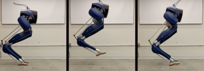
Figure 1: When legged robots such as Cassie execute agile high-impact motions like jumping, shown above, the joint velocities undergo rapid changes at the impact event. Attempting to apply feedback control on these velocities, using a reference trajectory that may be discontinuous due the rigid contact model assumption, is a difficult task. Often, the controller will actually introduce disturbances. This paper proposes a method to project both the robot velocities and the reference trajectory to a subspace that is invariant under impacts.

Tracking a discontinuous trajectory is problematic due to the unavoidable difference between the reference trajectory and actual system caused by even minuscule differences in impact timing. These differences cause feedback control efforts to spike, leading to instabilities. While these controller spikes can be reduced through strategies such as blending controller gains and contact constraints around the impact event [mason2016balancing], [atkeson2015no], these heuristic methods do not address the fundamental challenge of tracking discontinuous trajectories. A strategy that does attempt to directly addresses this challenge is termed reference spreading control [rijnen2017control]. This method leverages contact detection and extending the reference trajectories to ensure that a valid reference trajectory exists despite mismatches in impact timing. However, during the transition between contact modes when the impact is still resolving, tracking even the extended reference trajectories can be detrimental.

Alternate methods, we note, focus instead on avoiding impact events altogether. While impacts do not exist for frequently used templates such as the linear inverted pendulum (LIP) and the spring-loaded inverted pendulum (SLIP), impacts will manifest when embedding these templates onto physical robots with non-negligible mass in the legs. Furthermore, it is neither possible nor desirable to avoid impacts for more agile motions such as running or jumping. Thus, handling non-trivial impacts in a robust manner is essential to the development of more agile legged robots.

In this work, we propose a method for tracking discontinuous trajectories across impacts that directly avoids jumps in tracking error. We achieve this by projecting the tracking objectives down to a subspace where they are invariant to the impact event. Gong and Grizzle [gong2020angular] made an important insight about angular momentum about the contact point, noting that it is invariant to impacts at that contact point. Inspired by this, we generalize this property and extend it to include the entire invariant subspace, which we term the impact invariant subspace. The primary contribution of this paper is the identification of this subspace for the purposes of improving controller robustness to uncertainty in the impact event. We develop a method for adapting controller feedback to be applied only on this subspace of velocities that are invariant to any contact impulses. The subspace is easily defined for any legged robot at any given configuration, and the projection to that subspace can be applied to any tracking objective that is purely a function of the robot’s state. A key benefit of the impact invariant projection is that it enables controllers to be robust to uncertainty in the impact event, while minimally sacrificing control authority .

To demonstrate the directional robustness to uncertainty in the impact event, we apply the projection to a walking gait for a planar five link biped. Additionally we showcase the performance of the projection on an Operational Space Controller (OSC) tracking a jumping motion in simulation and on hardware for the bipedal robot Cassie.

II Background

II-A Rigid Body Dynamics

We use both the planar biped Rabbit [chevallereau2003rabbit] and the 3D complaint bipedal robot Cassie to demonstrate the benefits of the idea of impact invariance. Both legged robots are modeled using conventional floating-base Lagrangian rigid body dynamics. Cassie has passive springs on its heel and knee joints; for the purposes of modeling and control we treat these springs as rigid. However, when evaluating our results in simulation, we do include these terms.

The robot’s state $x\in\mathbb{R}^{2n}=\left[q;\dot{q}\right]$, described by its positions $q\in\mathbb{R}^{n}$ and velocities $\dot{q}\in\mathbb{R}^{n}$, is expressed in generalized floating-base coordinates. The dynamics are derived using the Euler-Langrange equation and expressed in the form of the general manipulator equation:

$$M(q)\ddot{q}+C(q,\dot{q})+g(q) =Bu+J_{\lambda}(q)^{T}\lambda,$$ (1)

where $M$ is the mass matrix, $C$ and $g$ are the Coriolis and gravitational forces respectively, $B$ is the actuator matrix, $u$ is the vector of actuator inputs, and $J_{\lambda}$ and $\lambda$ are the Jacobian of the holonomic constraints and corresponding constraint forces respectively.

II-B Rigid Body Impacts

In this paper, we model the complex deformations and surface forces when a legged robot makes contact with a surface using a rigid body contact model. This contact model does not allow deformations; instead, impacts are resolved instantaneously. Therefore, the configuration remains constant over the impact event and the velocities change instantaneously according to the contact impulse $\Lambda$:

$$M(\dot{q}^{+}-\dot{q}^{-}) =J_{\lambda}^{T}\Lambda,$$ (2)

where $\dot{q}^{+}$ and $\dot{q}^{-}$ are the pre- and post-impact velocities, and $\Lambda$ is the impulse sustained over the impact event. With the addition of a standard constraint that the new stance foot does not move once in contact with the ground (no-slip condition):

$$J_{\lambda}\dot{q}^{+}=0,$$ (3)

$\Lambda$ can be solved for explicitly, determining the post-impact state $x^{+}$ purely as a function of the pre-impact state $x^{-}$:

$$q^{+} =q^{-},$$ (4)

$$\dot{q}^{+} =(I-M^{-1}J_{\lambda}^{T}(J_{\lambda}M^{-1}J_{\lambda}^{T})^{-1}J_{\lambda})\dot{q}^{-}.$$ (5)

This reset map is conventionally enforced as a constraint between hybrid modes separated by an impact event for trajectory optimization of legged robots.

III Impact Invariance

To motivate the concept of the impact invariant subspace, we begin by highlighting and describing the difficulties of applying feedback control during an impact event. For the sake of simplicity, we consider a feedback controller with constant feedback gains that controls an output $y:\mathbb{R}^{n}\rightarrow\mathbb{R}^{d}$ to track a time-varying trajectory $y_{des}(t):~{}\left[0,\infty\right)\rightarrow\mathbb{R}^{d}$ by driving the tracking error $\tilde{y}(t)=~{}y_{des}(t)-y(t)$ to zero. This is commonly accomplished with a standard control law $u=u_{ff}+u_{fb}$ where $u_{ff}$ is the feedforward controller effort required to follow the reference acceleration $\ddot{y}_{des}$ and the $u_{fb}$ is the PD feedback component given by:

$$u_{fb}(t)=K_{p}\tilde{y}(t)+K_{d}\dot{\tilde{y}}(t).$$ (6)

Figure 2: Illustration of a reference trajectory with a discontinuity due to an impact and a system that seeks to track that discontinuous trajectory. The velocity error will spike unless the actual and nominal impact time match up perfectly.

The reference trajectory $\dot{y}_{des}(t)$ for systems that make contact with their environment has discontinuities at the impact events in order to be dynamically consistent with (5). Therefore, in a short time window around an impact event, there will be a discontinuity in the reference trajectory $\dot{y}_{des}(t)$ at the nominal impact time and another discontinuity when the actual system $\dot{y}(t)$ makes contact with the ground as shown in Fig. 2. Because the robot configuration is approximately constant over the impact event, the change in controller effort is governed by the change in velocity error:

$$\Delta u\approx K_{d}\Delta\dot{y},$$ (7)

thus any mismatches in impact timings will unavoidably result in spikes in the feedback error and therefore control effort as similarly noted in [rijnen2017control].

Remark 1

We make an assumption that the jump in the reference trajectory is time-based. Although it is possible to formulate trajectories with event-triggered jumps, these methods require detection, which for state-of-the-art methods still have delays of 4-5ms [bledt2018cheetah]. Moreover, in reality, impacts are not resolved instantaneously but rather over several milliseconds. In this time span, it is not clear which reference trajectory to use as using either trajectory will output a large tracking error.

Note that a large tracking error, shown in Fig. 2, results from only a small difference in impact timing, yet the controller will respond to the large velocity error and introduce controller-induced disturbances. This sensitivity to the impact event is amplified by the large contact forces that impair state estimation and inaccuracies in our contact models [fazeli2020fundamental], meaning that the velocities post-impact may not match up with the reference trajectory. Detecting the “true” error for discontinuous functions is a difficult problem and has been explored in [pfrommer2020contactnets].

The key insight in resolving this problem is inspired by [gong2020angular], in which Gong and Grizzle delineate desirable properties of angular momentum about the contact point, denoted as $L$. They highlight that $L$ is invariant over impacts on flat ground, meaning that it is continuous over the impact event despite it being a function of velocity.

The concept of an impact invariant subspace is a generalization of this property. We observe that there is a space of velocities that, like $L$, are continuous through impacts for any contact impulse. By switching to track these outputs in a small time window around anticipated impacts, we avoid controller-induced disturbances from uncertainty in the impact event. Note that while $L$ $\in\mathbb{R}^{3}$ or $\mathbb{R}^{2}$ for planar systems such as Rabbit, the impact invariant subspace $\in\mathbb{R}^{n-c}$, where $n$ is the dimension of generalized velocities and $c$ is the number of independent constraints of the impact event. For Rabbit, this space is $\in\mathbb{R}^{7-2}$. For Cassie, each foot provides 5 holonomic constraints and the four bar linkage on each leg provides 2 additional holonomic constraints that are always active. Therefore the impact invariant subspace is $\in\mathbb{R}^{18-7}$ for impacts with a single foot (walking, running) and $\in\mathbb{R}^{18-12}$ for impacts with both feet (jumping). A direct benefit of this higher dimensional space is the higher degree of possible control, which enables more agile or energetically efficient motions.

The impact invariant subspace is defined as the nullspace of $M^{-1}J_{\lambda}^{T}$, which is the matrix that maps contact impulses to generalized velocities. Thus a basis $P(q)\in\mathbb{R}^{(n-c)\times n}$ for this nullspace is such that:

$$P(\dot{q}-\dot{q}^{-})=0=PM^{-1}J_{\lambda}^{T}\Lambda.$$ (8)

This creates the intended effect, that is, for any contact impulse $\Lambda$, the impact invariant velocities will be unchanged. Alternatively, to project the generalized velocities down to the impact invariant subspace, we can simply create a low-rank $\mathbb{R}^{n\times n}$ projection matrix $Q(q)=P^{T}P$.

To illustrate the benefit on a physical robot, we apply the impact invariant projection to the joint velocities for Cassie executing a jumping motion right when it lands as shown in Fig. 3. Observe that the projected joint velocities are significantly smoother than the original joint velocities.

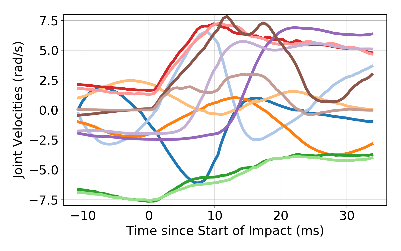
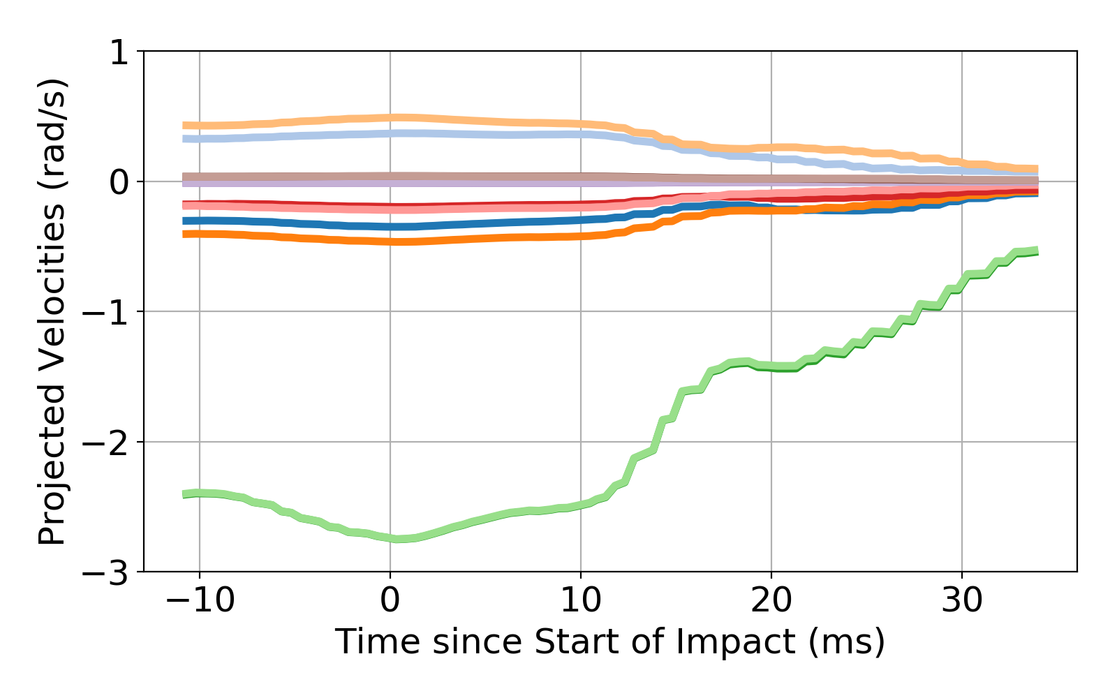
Figure 3: Demonstration of the impact invariant projection on joint velocity data from a successful jumping experiment on the physical Cassie robot. Joint velocities (top) during the landing event change rapidly which is difficult to perform feedback control on. By projecting the same joint velocities to the impact invariant subspace (bottom), the values are more consistent and more amenable for feedback control. Note, the change in joint velocities primarily occurs within a time span of only 10 ms. The L and R subscripts indicate the left and right leg respectively.

III-A Application to Joint Space Tracking

Many joint space controllers have been formulated for the control of bipedal robots. These include controller such as Hybrid LQR [mason2016balancing], joint PD control [gong2019feedback] [green2020learning], as well as inverse dynamics controllers that primarily track joint space outputs [reher2020inverse]. Utilizing the impact invariant projection on these controllers is straightforward. In a small time window around the anticipated impact, simply replace the original control law

$$u=u_{ff}+K_{p}\tilde{q}+K_{d}\dot{\tilde{q}},$$

with the new projected joint velocity error, which results in

$$u^{*}=u_{ff}+K_{p}\tilde{q}+K_{d}Q(q)\dot{\tilde{q}}.$$ (9)

III-B Application to Task Space Tracking

III-B1 Operational Space Controller

When the tracking objectives are instead more general functions of the robot’s state, this style of controller is commonly referred to as operational space control (OSC). An OSC is an inverse dynamics controller that tracks a set of task or output space accelerations by solving for dynamically consistent inputs, ground reaction forces, and generalized accelerations [wensing2013generation] [sentis2005control]. For an output position $y(q)=\phi(q)$ and corresponding output velocity $\dot{y}=J_{y}(q)\dot{q}$, where $J_{y}(q)=\frac{{\partial}\phi}{{\partial}q}$, the commanded output accelerations $\ddot{y}_{cmd}$ are calculated from the feedforward reference accelerations $\ddot{y}_{des}$ with PD feedback:

$$\ddot{y}_{cmd} =\ddot{y}_{des}+K_{p}(y_{des}-y)-K_{d}(\dot{y}_{des}-\dot{y})$$ (10)

The objective of the OSC is then to produce dynamically feasible output accelerations $\ddot{y}$ given by:

$$\ddot{y} =\dot{J}_{y}\dot{q}+J_{y}\ddot{q},$$

such that the instantaneous output accelerations of the robot are as close to the commanded output accelerations as possible. This controller objective can be nicely formulated as a quadratic program:

$$\min_{u,\lambda,\ddot{q}} \sum_{i}^{N}({\ddot{y}_{i}-\ddot{y}_{i_{cmd}}})^{T}W_{i}(\ddot{y}_{i}-\ddot{y}_{i_{cmd}})$$ (11)

subject to: Dynamic Constraints (12)

Holonomic Constraints (13)

$$\text{Friction Cone Constraints}.$$ (14)

$i$ denotes the particular output being tracked (e.g., center of mass or foot position) and $W_{i}$ are corresponding weights on the tracking objectives.

III-B2 Projecting Outputs to the Impact Invariant Subspace

The desired and actual positional outputs $y_{des}$ and $y$ are trivially continuous over impacts. Thus, the impact invariant projection is applied only to the output velocities $\dot{y}$ and $\dot{y}_{des}$. However, due to the lack of a one-to-one mapping between output velocities $\dot{y}$ and generalized velocities $\dot{q}$, the projection in (8) cannot be naively applied. Still, it is possible to project the output velocity to a subspace so that it is invariant to any unknown contact impulse. In practice, this can be accomplished for a single output with the following optimization problem:

$$\min_{\lambda}\quad\left\lVert\dot{y}_{des}-J_{y}(\dot{q}+M^{-1}J_{\lambda}^{T}\lambda)\right\rVert_{2}.$$ (15)

This applies a correction to the generalized velocities $\dot{q}$ that minimizes the tracking error in the output velocities, under the condition that the correction lies within the set of feasible velocities that could result from a contact impulse $\lambda$. In the absence of constraints on $\lambda$, this can be formulated as a least squares problem and the optimal $\lambda$ can be solved for implicitly with the Moore-Penrose pseudo-inverse denoted by $(\cdot)^{\dagger}$. The projected output velocity error, $\dot{y}_{proj}$, can then be found as:

$$\dot{y}_{proj} =\dot{y}_{des}-J_{y}\dot{q}-J_{y}\dot{q}_{\lambda},$$ (16)

where the correction $\dot{q}_{\lambda}$ is given by:

$$\dot{q}_{\lambda} =M^{-1}J_{\lambda}^{T}(J_{y}M^{-1}J_{\lambda}^{T})^{\dagger}(\dot{y}_{des}-J_{y}\dot{q}).$$ (17)

This projected error $\dot{y}_{proj}$ is then used in place of the original output velocity error $\dot{y}_{des}-\dot{y}$ in (10). This can have two interpretations. One interpretation, which is more literal, is that we apply a correction in the space of $\lambda$ that minimizes the velocity tracking error in the output space. The other interpretation, is that the correction projects the velocity tracking error to the impact invariant subspace by eliminating the sensitivity of the error on $\lambda$. In either interpretation, it is easy to see that $\dot{y}_{proj}$ is invariant to any unknown contact impulse. Note, the solution to the least squares problem, $\lambda$, is not intended to be most physically plausible contact impulse, but instead the impulse that minimizes the tracking error. In both interpretations, the projection assumes an optimistic correction in the $\lambda$ space. Related work has also explored incorporating potential impacts into robust control formulations [wang2019impact]. A primary distinction is that [wang2019impact] seeks to be robust to impulsive impacts from a known model but at unexpected times, where our approach makes no assumptions on the magnitude or duration of impact forces.