Hydrodynamic non-linear response of interacting integrable systems

Abstract

We develop a formalism for computing the non-linear response of interacting integrable systems. Our results are asymptotically exact in the hydrodynamic limit where perturbing fields vary sufficiently slowly in space and time. We show that spatially resolved nonlinear response distinguishes interacting integrable systems from noninteracting ones, exemplifying this for the Lieb-Liniger gas. We give a prescription for computing finite-temperature Drude weights of arbitrary order, which is in excellent agreement with numerical evaluation of the third-order response of the XXZ spin chain. We identify intrinsically nonperturbative regimes of the nonlinear response of integrable systems.

Studying the response of a system to external fields yields information on its macroscopic order as well as its microscopic properties. While working to linear order in field strength often suffices to describe experiments, recent advances allow measurements to probe beyond the linear regime. Understanding nonlinear response functions could significantly advance the characterization of exotic phases of matter, but little is known theoretically about their properties in interacting many-body systems. We introduce a framework for computing non-linear responses in a class of exactly solvable one-dimensional quantum systems. We show that non-linear response exhibits clear signatures of interaction effects, in contrast to linear response in similar settings.

I Introduction

Most conventional experimental probes of many-body systems, from spectroscopy to transport, operate in the linear-response regime. Linear-response coefficients such as the a.c. conductivity and dynamical susceptibility have a natural theoretical interpretation in terms of the fluctuation-dissipation theorem Martin (1968): the response to an external probe captures the intrinsic fluctuations of the system’s degrees of freedom. Despite its many successes, linear response has its limitations as a probe of correlated quantum matter. For example, many different mechanisms — of varying levels of interest — give rise to incoherent spectral continua, and cannot be differentiated on the basis of linear-response data. Likewise, quantities like the conductivity probe some specific combination of the density and lifetimes of excitations; thus, e.g., the finite-frequency conductivity is qualitatively the same for a metal and an insulator. Recently, various experimental probes of nonlinear response have been developed to circumvent these difficulties, ranging from quench experiments in ultracold atomic gases Bloch et al. (2008) to pump-probe spectroscopy Cavalleri et al. (2001) and multidimensional coherent spectroscopy Mukamel (1999); Lynch et al. (2010); Lu et al. (2016); Hirori et al. (2011); Kuehn et al. (2011); Jepsen et al. (2001); Woerner et al. (2013); Lu et al. (2017); Mahmood et al. (2021); Wan and Armitage (2019); Parameswaran and Gopalakrishnan (2020); Nandkishore et al. (2021); Nandkishore and Gopalakrishnan (2021); Michishita and Peters (2020); João and Lopes (2019); Choi et al. (2020); Kanega et al. (2021); Holsten and Krüger (2021); Paul (2021) in condensed-matter settings. While the first of these methods is apt for probing far-from-equilibrium dynamics and the second radically reconstructs the state of the system, the third is milder, and probes higher-order and multiple-time correlations of the equilibrium system. Such nonlinear probes are able to distinguish phases that have similar linear-response signatures: e.g., they can distinguish between excitation broadening due to disorder and that from decay Mahmood et al. (2021). Despite a flurry of recent work Sodemann and Fu (2015); Wan and Armitage (2019); Parameswaran and Gopalakrishnan (2020); Parker et al. (2019); Nandkishore et al. (2021); Li et al. (2020); Nandkishore and Gopalakrishnan (2021); Michishita and Peters (2020); João and Lopes (2019); Choi et al. (2020); Kanega et al. (2021); Holsten and Krüger (2021); Paul (2021), the theoretical toolbox for addressing nonlinear response in generic interacting quantum many-body systems is primitive, with few exact results beyond free theories and those that reduce to ensembles of two-level systems. (Notable exceptions are Refs. Doyon and Myers (2019); Myers et al. (2020); Perfetto and Doyon (2020) which compute specific time-ordered $n$-point correlation functions in integrable systems with the goal of characterizing ballistic transport.)

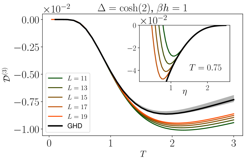
Figure 1: Third-order spin Drude weight $\mathcal{D}^{(3)}$ in the easy-axis regime of the XXZ spin chain with $\beta h=1$. Main figure: Comparison between GHD and ED results for fixed $\Delta$. The lower (upper) boundaries of the shaded region correspond to extrapolations of finite-size ED results with a degree $1$ (degree $2$) polynomial in $1/L$. Inset: $\mathcal{D}^{(3)}$ as a function of $\eta=\cosh^{-1}\Delta$.

Here, we develop and apply an asymptotically exact framework for computing the nonlinear response of interacting integrable systems, i.e. those solvable by the thermodynamic Bethe ansatz (TBA) Takahashi (2005). This framework is based on viewing integrability through the lens of generalized hydrodynamics (GHD) Castro-Alvaredo et al. (2016); Bertini et al. (2016); Doyon (2020) (see also Sachdev and Damle (1997); Damle and Sachdev (1998) for a precursor of this approach, and e.g. Doyon and Yoshimura (2017); Doyon and Spohn (2017); Ilievski and De Nardis (2017); Bulchandani et al. (2017); Piroli et al. (2017); Alba and Calabrese (2017); Doyon et al. (2018, 2017); Cao et al. (2018); Bastianello et al. (2019); De Nardis et al. (2018); Gopalakrishnan et al. (2018); Bastianello et al. (2020); Caux et al. (2019); Møller et al. (2020); Koch et al. (2020); Pozsgay (2020); Borsi et al. (2020); Friedman et al. (2020); Durnin et al. (2020); Fava et al. (2020); Schemmer et al. (2019); Malvania et al. (2020) for recent developments); our results are exact at the hydrodynamic Euler scale, i.e. for perturbations that vary slowly in space and time. [The response to sharply localized potentials could contain oscillations in space and time that the GHD approach automatically averages out and hence cannot properly capture.] We remark that with these caveats GHD, and thus our method, is believed to be exact at any finite temperature and it can be applied to the computation of correlation functions of the density of any conserved charge in any integrable system.

In the present work, we show that the nonlinear response of integrable systems contains information that is absent from (or subleading in) linear response: while the spectral functions of free and interacting integrable systems are qualitatively similar (with only subtle differences in the broadening around their ballistic light-cones Gopalakrishnan et al. (2018); De Nardis et al. (2018)), we find that spatially resolved nonlinear response reveals clear, qualitative distinctions between interacting and noninteracting integrable systems (as well as between chaotic and integrable systems). We discuss the prospects for measuring these features in experiments on interacting many-particle systems using nonlinear spectroscopic probes.

We also consider the generation of persistent currents after the application of an electric field, which is one of the hallmarks of integrability. At linear order in the field, the current is encoded in the linear Drude weight Doyon and Spohn (2017); Ilievski and De Nardis (2017). This can be readily generalized beyond the linear order, by defining higher-order Drude weights $\mathcal{D}^{(n)}$ Watanabe and Oshikawa (2020); Watanabe et al. (2020). We show that our formalism yields a compact recursive formula for $\mathcal{D}^{(n)}$ at finite temperatures. We demonstrate the validity of our hydrodynamic approach by comparing its results with those of exact diagonalization studies of integrable spin chains; we find excellent agreement (Fig. 1). We conclude by discussing the special case of the isotropic Heisenberg chain, which is known to host anomalous superdiffusive transport Ljubotina et al. (2017); Ilievski et al. (2018); Gopalakrishnan and Vasseur (2019); De Nardis et al. (2019a); Ljubotina et al. (2019); Bulchandani (2020); De Nardis et al. (2020) characterized by propagation that is slower than ballistic motion but faster than diffusion. We show that the emergence of supediffusion is accompanied by a breakdown of perturbation theory in the external field and hence an inherently non-perturbative nonlinear response.

II Setup

We consider general one-dimensional systems whose dynamics are governed by some integrable Hamiltonian $H_{0}$. The dynamics under $H_{0}$ are treated within Euler-scale GHD Doyon (2020): we partition the system into hydrodynamic cells each of mesoscopic size and linked to some spacetime point $(x,t)$, and assume that each cell is always instantaneously in some local generalized Gibbs ensemble (GGE) Rigol et al. (2007); Luca D’Alessio and Yariv Kafri and Anatoli Polkovnikov and Marcos Rigol (2016), characterized by the vector of occupation factors of available quasiparticle states, $\boldsymbol{n}(x,t)=\{n_{\theta}(x,t)\}$; the “rapidity” $\theta$ is a convenient way of parameterizing the momentum. (We present results for systems with a single quasiparticle species but the generalization to multiple species is immediate.) The density of quasiparticles of species $\theta$ can be expressed in terms of $\boldsymbol{n}$ as $\rho_{\theta}\equiv\rho^{t}_{\theta}n_{\theta}$, where $\rho^{t}_{\theta}$ is the available density of states for quasiparticles with those quantum numbers. (Note that, in an interacting system, $\rho^{t}_{\theta}$ is itself a nontrivial function of the local GGE.) Because of integrability, $\rho_{\theta}$ is separately conserved for each $\theta$; moreover, $n_{\theta}$ obeys a quasilinear advection equation,

$$\partial_{t}n_{\theta}+v^{\mathrm{eff}}_{\theta}[\boldsymbol{n}]\partial_{x}n_{\theta}=0,$$ (1)

where $v^{\mathrm{eff}}_{\theta}$ is an effective group velocity. In non-interacting systems, the effective velocity $v^{\text{eff}}$ of a quasiparticle is just its group velocity. In an interacting integrable system, however, collisions are associated with a time delay in the quasiparticle trajectory, and thus renormalize the effective quasiparticle velocity. $v^{\text{eff}}$ is therefore a nonlinear functional of $\boldsymbol{n}$.

$H_{0}$ has an infinite set of conserved charges, $[H_{0},\hat{Q}^{j}]=0$, whose expectation values in a GGE state are given by $\langle\hat{Q}^{j}\rangle=\int dx\langle\hat{q}_{j}\rangle=\int dxd\theta\,q^{j}_{\theta}\rho_{\theta}$, where $q^{j}_{\theta}$ is the contribution to the $j^{\text{th}}$ charge density from quasiparticle $\theta$. The corresponding current density is $j_{j}=\int d\theta\rho_{\theta}q^{j}_{\theta}v^{\mathrm{eff}}_{\theta}$. GHD is highly nonlinear, even at the Euler scale, since the properties of each quasiparticle are strongly renormalized by its interactions with all the others; however, this nonlinearity can be addressed using TBA techniques.

Figure 2: Four distinct physical processes contributing to the second-order response $\chi^{(2)}$. (a) A thermal quasiparticle (QP; black line) is accelerated twice by the electric field (red wavy line), and modifies the expectation value $\langle\hat{O}\rangle$ in the final space-time cell. (b) First a thermal QP is accelerated; a second thermal QP (blue line) is later accelerated when the first is in its space-time cell, thus modifying the effective acceleration perceived by the second; both QPs proceed ballistically and the second modifies $\langle\hat{O}\rangle$. (c) Two thermal QPs are independently accelerated by two pulses of the electric field; after travelling to the same space-time cell, and together they modify $\langle\hat{O}\rangle$. (d) As in (c), two thermal QPs are independently accelerated but one scatters off the other before influencing $\langle\hat{O}\rangle$. Only (a) is relevant to free systems but all four processes contribute in interacting integrable systems.

We now discuss how external forces can be incorporated into GHD Doyon and Yoshimura (2017); Bastianello et al. (2019). For concreteness we specialize to the case where the coupling is to a global $U(1)$ charge $\hat{q}=\hat{q}_{0}$, which remains conserved even in the presence of inhomogeneous fields. Thus, the perturbed Hamiltonian is ${H}(t)=\hat{H}_{0}+\int dx\,V(x,t)\hat{q}_{0}(x)$. Assuming $V$ varies slowly in space and time, the Euler-scale time evolution of the system is described by Doyon and Yoshimura (2017); Cao et al. (2018); Bastianello et al. (2019, 2020); Caux et al. (2019); Møller et al. (2020); Koch et al. (2020)

$$\partial_{t}n_{\theta}+v^{\text{eff}}_{\theta}\partial_{x}n_{\theta}+Ea_{\theta}^{\text{eff}}\partial_{\theta}n_{\theta}=0,$$ (2)

where $a_{\theta}^{\text{eff}}[\boldsymbol{n}]$ is the effective acceleration of the quasiparticles, and the sole dependence on the potential is via the electric field $E(x,t)\equiv-\partial_{x}V(x,t)$. As is the case for $v^{\text{eff}}$, $a^{\text{eff}}$ is also renormalized by scattering processes and is hence a nonlinear functional of $\boldsymbol{n}$.

Finally, we note that (2) is strictly valid only at the Euler scale, i.e., for response at asymptotically large $x$ and $t$, but with a fixed ratio $x/t$. Euler-scale response is a hallmark of integrable dynamics: chaotic systems without Galilean invariance have exponentially suppressed response at the Euler scale, since densities spread diffusively rather than ballistically. Interacting integrable systems also have diffusive corrections to ballistic quasiparticle spreading De Nardis et al. (2018); Gopalakrishnan et al. (2018); De Nardis et al. (2019b), but these corrections are also suppressed at the Euler scale.

III Nonlinear-response

Response is concerned with computing the value of some local observable $\hat{O}$—taken here to be a charge density $\hat{q}_{j}$ or current density $\hat{j}_{j}$—following the application of electric fields $E(x,t)$. Since (2) is asymptotically exact at the Euler scale to all orders in $V_{j}$, it is sufficient to work perturbatively in $V_{j}$ to compute the response (we comment on exceptions below). Formally, the connected order-$N$ response is

$$\chi^{(N)}_{\hat{O}}\left(\{x_{n},t_{n}\}\right)=\left.\prod_{n=0}^{N-1}\frac{\delta}{\delta E(x_{n},t_{n})}\langle\hat{O}(x_{N},t_{N})\rangle\right|_{E\to 0}$$ (3)

with $t_{0}<t_{1}<\cdots<t_{N}$. The expectation value is taken with respect to the nonuniform state at time $t_{N}$ generated by perturbing the initial uniform GGE state with external fields at times $t_{1},\ldots t_{N-1}$. Our strategy is to express the expectation value in (3) in terms of quasiparticle occupations, perform all the functional derivatives, and then set $E=0$, yielding an expression that we evaluate in the uniform GGE.

An expectation value $\langle O(x,t)\rangle$ is a nonlinear functional of the local state $\boldsymbol{n}(x,t)$. It can be affected by perturbations at other spacetime points only through the advection of those perturbations to $(x,t)$, which is captured by the propagator $D_{\theta\theta^{\prime}}(z,z^{\prime})=\frac{\delta n_{\theta}(z)}{\delta n_{\theta^{\prime}}(z^{\prime})}$, where we have defined $z\equiv(x,t)$. One can express this dependence in the following compact form, suggestive of a chain rule Doyon (2018a):

$$\frac{\delta\langle\hat{O}(z_{1})\rangle}{\delta E(z_{0})}=\!\int\!\!d\theta d\alpha\frac{\delta\langle\hat{O}(z_{1})\rangle}{\delta n_{\alpha}(z_{1})}\frac{\delta n_{\alpha}(z_{1})}{\delta n_{\theta}(z_{0})}\frac{\delta n_{\theta}(z_{0})}{\delta E(z_{0})},$$ (4)

(4) simply says that expectation values at spacetime point $z_{0}$ depend on fields at $z_{1}\neq z_{0}$ purely via the process by which the fields perturb the quasiparticle distribution at $z_{0}$ and this perturbation is advected over to $z_{1}$.

We are interested in generalizing (4) to the case of higher-order functional derivatives. To organize these more complicated expressions we have developed a diagrammatic framework SM , which relies on the observation that any functional derivative can be composed of the following types of elementary object. First, there are propagators, defined above, connecting perturbations at different spacetime points; in a uniform GGE, the propagators take the simple form $D_{\theta\theta^{\prime}}(x_{0},t_{0};x_{1},t_{1})=\delta_{\theta\theta^{\prime}}\delta\left[(x_{0}-x_{1})-v^{\mathrm{eff}}_{\theta}(t_{0}-t_{1})\right]$ Doyon (2018b). Second, there are functional derivatives of observables at a point with respect to the quasiparticle distribution at the same point, which can be evaluated using TBA techniques Doyon (2020). We call these “measurement vertices.” Third, there are derivatives of the quasiparticle distribution at a spacetime point with respect to fields at the same point. To find these we invert (2) using Green’s function techniques, and thereby find $\frac{\delta n_{\theta}(z)}{\delta E(z)}=-a^{\text{eff}}_{\theta}[\boldsymbol{n}]\partial_{\theta}{n}_{\theta}$ SM . We term these objects “field vertices.” These three types of objects appear in (4). Finally, response functions at order $N>1$ will also involve expressions of the form $\Gamma^{(p)}=\frac{\delta^{p}n_{\theta}(z_{0})}{\delta n_{\theta_{1}}(z_{1})\ldots\delta n_{\theta_{p}}(z_{p})}$. These capture the modification of the spacetime propagator by scattering events, and can be computed by repeatedly differentiating (1) with respect to $n$, which yields a recursive formula, that allows us to express $\Gamma^{(p)}$ in terms of $\partial_{x}\Gamma^{(1)}$ and functional derivatives of the $v^{\text{eff}}[\boldsymbol{n}]$ with respect to quasiparticle occupations SM . We refer to these objects as “scattering vertices.” All other types of object can be expressed in terms of these: e.g., functional derivatives of the form $\frac{\delta^{k}\langle\hat{O}\rangle}{\delta n_{\theta_{1}}(z_{1})\ldots\delta n_{\theta_{k}}(z_{k})}$, can be rewritten in terms of measurement or scattering vertices and propagators, which advect all occupation factors to the point where the functional derivative is taken. We may verify that for $N=1$ this procedure yields the standard expressions for linear response. Higher-order response functions can then be computed recursively from (3).

Although the formal expressions rapidly become unwieldy with increasing $N$, they have a transparent physical interpretation, as we now exemplify for $N=2$. The external field can affect the system via two distinct physical processes, each corresponding to a distinct field vertex (represented by a box with a wavy line in Fig. 2): it can accelerate a thermal quasiparticle from rest within a spacetime cell (the first field vertex in Fig. 2a), or else accelerate a quasiparticle previously acted upon by the field at an earlier time (the second field vertex in Fig. 2a). In a non-interacting integrable system different quasiparticles are independent of each other, thus all connected nonlinear response functions result solely when a single quasiparticle is repeatedly accelerated by the field, and then measured, as in Fig. 2a. However, in interacting integrable systems, quasiparticles influence each other via scattering processes. Consequently, the ability of the field to excite a quasiparticle in a given spacetime cell $z$ is also sensitive to the presence of quasiparticles excited by the field in all spacetime cells in the past light-cone of $z$ under the advective dynamics of GHD, leading to additional connected contributions (as in Fig. 2b). Quasiparticles excited by the field acting at distinct spacetime cells can also propagate to a single cell where they jointly modify the measured observable (Fig. 2c). Interactions thus lead to an infinite hierarchy of field and measurement vertices, that are sensitive to the presence of an increasing number of previously-excited quasiparticles in the spacetime cells where quasiparticles are accelerated or measured. Finally, the nonlinear response also receives contributions from scattering vertices, again of arbitrary order, due to the phase shift experienced by the measured quasiparticle as it propagates between the acceleration and measurement cells in the presence of other excited quasiparticles in the system (Fig. 2d). The $N^{\text{th}}$ order response in an interacting integrable system involves $N$ field vertices and a single measurement vertex, linked by advection propagators $D_{\theta\theta^{\prime}}(z,z^{\prime})$ and scattering vertices, and can be organized using spacetime diagrams SM . Crucially, at fixed $N$, only vertices below some finite order can contribute: for instance Fig. 2 contains all processes contributing to $\chi^{(2)}$.

We caution the reader that in Fig. 2 the effects of fields and collisions are exaggerated for clarity. In fact, the trajectory shift due to scattering processes as in Fig. 2d is infinitesimal, and similarly a perturbing external field only imparts an infinitesimal acceleration to each quasiparticle. Thus there are kinematic restrictions on allowed processes that the figure does not capture. For instance, the process in Fig. 2a is possible only if the three points — the two where the field act and the one at which the measurement occurs — lie on the same ray $x=x_{0}+v_{\lambda}t$ for some initial position $x_{0}$ and some rapidity $\lambda$. This aspect will be crucial to our discussion in the next section.

IV Measuring Interactions in the Lieb-Liniger Gas

As an example of this approach, we apply it to the Lieb-Liniger model of 1D bosons with contact interactions,

$$\hat{H}_{0}=\frac{1}{2}\sum_{j}\hat{p}_{j}^{2}+c\sum_{i\neq j}\delta(\hat{x}_{i}-\hat{x}_{j}),$$ (5)

where $\hat{x}_{j}$ and $\hat{p}_{j}$ are the position and momentum of particle $j$. The bare group velocity $v$ of a particle is equal to its momentum $p$. The effective velocity $v^{\text{eff}}$ can be obtained from $v$ as the solution to an integral equation, whose explicit form is provided in the Methods section. An additional fact, peculiar to the Lieb-Liniger gas, is that the effective acceleration $a^{\text{eff}}$ is not renormalized by interactions; with our choice of conventions, $a^{\text{eff}}=1$. For $c\to 0$, $\hat{H}_{0}$ is a free Bose gas, while for $c\to\infty$ it can be described as a theory of free fermions. This can be recognized, for example, by studying $v^{\text{eff}}$, which in both limits tends to the bare group velocity $v$. Consequently linear response in these two limits approximates that of free bosons or fermions respectively, with only quantitative corrections from interactions. This hinders a precise measurement of $c$ based only on linear response. We now demonstrate that a spatially-resolved measurement of $\chi^{(2)}$ —or higher-order responses— carries direct information about the interactions. For concreteness, we consider a specific charge response of the form $\tilde{\chi}^{(2)}(x,t,\tau)\equiv\chi^{(2)}_{\hat{q}_{0}}(0,0;x,\tau;0,\tau+t)$ where the first perturbation and the measurement coincide spatially, and the system is perturbed at an intermediate time at position $x$. In the free boson or free fermion limits, we know from the discussion in the previous section that the only process contributing to $\chi^{(2)}$ is one where a single quasiparticle is repeatedly accelerated by the subsequent field applications (Fig. 2a). Furthermore, as previously noted, this process can take place only if all the points in which the perturbation is applied and the measurement point lie on the same ray. Thus, in the two non-interacting limits $\tilde{\chi}^{(2)}(x,t,\tau)$ will vanish everywhere except at $x=0$. Conversely, if $c=O(1)$, quasiparticles are strongly interacting, and each influences the dynamics of the others. For example, processes such as those in Fig. 2d will be non-zero since $v^{\text{eff}}$ of a quasiparticle with momentum $p$ will depend on all the quasiparticles in the same region. SM We thus expect that $\chi^{(2)}$ is generically finite and non-zero for arbitrary perturbation and measurement points.

To summarize: if we focus on the region away from $x=0$, i.e. chosen to exclude the case where all points lie along the same ray, we expect $\tilde{\chi}^{(2)}(x,t,\tau)$ to be directly sensitive to the interactions, and hence generically will have a nonzero value away from the free limits $c\to 0$ or $c\to\infty$. An immediate corollary is that in these limits, $\tilde{\chi}^{(2)}(x\neq 0,t,\tau)$ should respectively vanish as $O(c)$ or $O(1/c)$. This should be contrasted with linear response measurements where $\chi^{(2)}=O(1)$ in all these cases and the effect of interactions is to determine sub-leading corrections.

Indeed, this response is readily computed using the above formalism (as detailed in the Methods section and SM ); Fig. 3 shows the results for various interaction strengths, at fixed temperature $T$ and boson density $\bar{n}$. As $c$ decreases we see that the signal moves closer to $x=0$. This is because for $c\to 0$ the system is proximate to a Bose-Einstein condensate at $c=0$ and $T=0$ (see e.g. Refs. Takahashi (1999); Jiang Yu-Zhu (2015)), and hence only slow, low momentum quasiparticle states are occupied. [See the Methods for another effect contributing to the signal moving near $x=0$.] Furthermore, note that the signal starts to decrease either for $c\lesssim 10^{-2}$ or $c\gtrsim 1$, as expected. [Recovering free boson response as $c\to 0$ requires studying very low $c$; as $c$ decreases, the density of states initially increases due to the incipient Bose condensation, enhancing interaction effects.] These observations are not restricted to the protocol analyzed above: any protocol which separates the same-ray ‘free’ contribution from the regular part of the response would yield similar results. Thus, nonlinear correlators provide a more direct window into the interacting Lieb-Liniger gas than linear response.

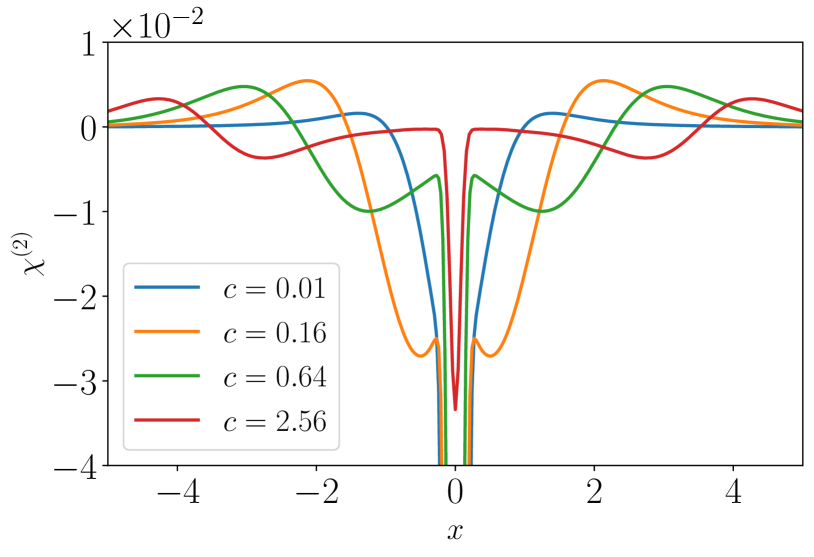
Figure 3: $\chi^{(2)}(0,0;x,\tau;0,\tau+t)$ in the Lieb-Liniger model for various interaction strengths $c$. We take $T=2$, $\bar{n}=1$, $\tau=t=1$ and regularize the $\delta$-function GHD propagator as a Gaussian of width $\eta=0.1$. In a noninteracting system, the only response would come from the resolution-limited spike at $x_{1}=0$; everything else is a signature of interactions.

In passing, note that spatially-resolved measurements of multi-point nonlinear response would also give a powerful diagnostic for ballistic transport, and hence integrability. As we remarked above, the existence of nontrivial Euler-scale response—absent strict Galilean invariance—is a hallmark of integrable dynamics, and suffices to diagnose integrability. Even in Galilean-invariant chaotic fluids with a few conserved currents, quasiparticles propagate sub-ballistically, so one expects an Euler-scale multi-point correlator like that shown in Fig. 3 to be strongly suppressed relative to the integrable case.

V Higher-order Drude weights

So far, we have focused on spatially-resolved response. While this can be measured in cold-atom experiments, most solid-state spectroscopic techniques only access spatially integrated quantities. At the Euler scale, the most natural integrated quantity is the generation of a persistent current in response to a uniform electric field. This follows from the fact that the current operator in an integrable system generically has some part that is strictly conserved under time evolution, so the current generated in response to an electric field will not decay over time. For example, specializing to first-order response, $\int dx\,\chi^{(1)}_{\hat{j}_{0}}(0,0;x,t)$ will tend to a constant as $t\to\infty$; this limiting value is called the Drude weight Bertini et al. (2021); Prosen (2011). Alternatively, in frequency space, the conductivity goes as $\sigma(\omega)=\pi\mathcal{D}\delta(\omega)+\ldots$. Drude weights extend to nonlinear response: a field $E$ applied to the system for a finite time $\Delta t$ drives a persistent current $j_{0}(\varphi)$, where $\varphi\equiv E\Delta t$ is the vector potential variation due to the field. By expanding $j_{0}(\varphi)$ as a series in its argument and taking derivatives, we may define a sequence of nonlinear Drude weights Watanabe and Oshikawa (2020); Watanabe et al. (2020) (which can be defined similarly for any other operator).

Our diagrammatic approach can straightforwardly be used to compute $N^{\text{th}}$ order Drude weights $\mathcal{D}^{(N)}$, by integrating the $N^{\text{th}}$ order response over the positions of the field insertions. As shown in the SM SM , this yields the recursive formula

$$\mathcal{D}^{(N)}_{\hat{O}}=-\int d\theta_{N}a^{\text{eff}}\partial_{\theta_{N}}n\frac{\delta}{\delta n_{\theta_{N}}}\mathcal{D}^{(N-1)}_{\hat{O}},$$ (6)

with $\mathcal{D}^{(0)}=\langle\hat{O}\rangle$. This recursive formula allows to obtain a closed-form expression for non-linear Drude weight of arbitrary order only using TBA technology, with explicit expressions up to third order given in the SM SM .

While (6) rapidly becomes complex with increasing $N$, a simple limit emerges for the first term of a high-temperature expansion: since each factor of $\partial_{\theta}n$ is proportional to $T^{-1}$, the leading contribution to $\mathcal{D}^{(N)}_{\hat{O}}$ is always obtained by acting with $\frac{\delta}{\delta n_{\theta_{N}}}$ on the factor $\partial_{\theta_{N-1}}n_{\theta_{N-1}}$ in $\mathcal{D}^{(N-1)}_{\hat{O}}$. Integrating by parts, we find that as $T\to\infty$,

$$\mathcal{D}^{(N)}_{\hat{O}}=-\int d\theta\partial_{\theta}n\left[a^{\text{eff}}\frac{\partial}{\partial\theta}\right]^{N-1}a^{\text{eff}}\frac{\delta\langle\hat{O}\rangle}{\delta n(\theta)}+O(T^{-2}).$$ (7)

We benchmark this GHD result against numerical simulations of a paradigmatic integrable model, the XXZ spin chain, and focus on spin current response. Since spatial inversion symmetry forces spatially-averaged current response functions to vanish for any even $N$, we focus on $\mathcal{D}^{(3)}$. We work in the easy-axis limit, and exploit the generalized Kohn formula Watanabe and Oshikawa (2020); Watanabe et al. (2020) combined with exact diagonalization (ED) on small systems. (Unfortunately, state-of-the-art matrix product operator techniques for linear Drude weights Karrasch et al. (2012) do not give comparably good results for higher-order Drude weights SM .) Our results are presented in Fig. 1; despite the difficulty of extrapolating reliably to the thermodynamic limit from the small system sizes accessible to ED, we see that the GHD results are within the range of our extrapolations at high temperature, and agree extremely well at lower temperatures. We also see good agreement as we vary the easy-axis anisotropy at fixed temperature.

VI Discussion

In this work we have presented a general framework for computing nonlinear response within GHD, demonstrated that it is in excellent agreement with exact numerics, and illustrated how it can directly distinguish between free and interacting integrable systems. Our results suggest a natural experimental protocol for directly measuring quasiparticle interaction effects in the Lieb-Liniger model using ultracold atomic gases. (Importantly, this approach does not require single-site imaging resolution.) Since our proposal involves finite-time behavior, it can be applied to realistic experimental settings where integrability is only approximate. We have focused on regimes where the nonlinear response is perturbative, and can be expanded in powers of the field strength. In such regimes, our results for nonlinear response bear some resemblance to those for full counting statistics Doyon and Myers (2019); Myers et al. (2020); Perfetto and Doyon (2020). The multipoint correlators that appear in that theory (with all operators evaluated at the same point in space) are a special case of those computed here.

We need not look far for integrable systems in which response is inherently nonperturbative. The most transparent example is the isotropic Heisenberg model, at $h=0$. In linear response, this model exhibits anomalous transport in the Kardar-Parisi-Zhang universality class Ljubotina et al. (2017); Ilievski et al. (2018); Gopalakrishnan and Vasseur (2019); De Nardis et al. (2019a); Ljubotina et al. (2019); Bulchandani (2020); De Nardis et al. (2020). We may approach this regime from nonzero $\beta h$ by taking appropriate limits. Explicitly computing the spin current due to an impulse $\varphi=E\Delta t$, we find that

$$J(h,\varphi)\approx h\sum_{s=1}^{1/h}s^{-4}f(h\varphi s^{3}),$$ (8)

for some scaling function $f$ that is approximately sinusoidal in its argument SM . The sum is over quasiparticle “strings”, which are bound states of $s$ elementary magnons. If we now take $\varphi\to 0$ at fixed $h\neq 0$, we obtain a series in powers of $\varphi$, where the first term is the linear Drude weight ($\varphi\mathcal{D}^{(1)}\sim\varphi h^{2}|\log h|$), the next nonvanishing term is $\mathcal{\varphi}^{3}\mathcal{D}^{(3)}\sim\varphi^{3}/h^{2}$, and higher-order terms are even more singular in the half-filling limit. The $\varphi\to 0$ and $h\to 0$ limits strikingly fail to commute: if we instead take $h\to 0$ at fixed $\varphi$, we find that $J(h,\varphi)\sim h^{2}\varphi|\log h\varphi|$. In effect, $\varphi$ can act as a cutoff on response: for any fixed field, sufficiently large bound states respond nonperturbatively and undergo Bloch oscillations. A proper description of such nonperturbative phenomena requires extending the present framework beyond Euler scale, e.g., by including diffusive corrections De Nardis et al. (2018); Gopalakrishnan et al. (2018); De Nardis et al. (2019b) and other sources of irreversibility Bastianello and De Luca (2019). We leave this as an important direction for future work.

Note added.— As this paper was being completed we became aware of recent work Tanikawa et al. (2021) that computes exact non-linear Drude weights for the XXZ chain. Ref. Tanikawa et al. (2021) considers only $T=0$ and $|\Delta|<1$, and hence has limited overlap with the results presented here. We have checked that our results for $T\to 0$ agree in the relevant regime of $\Delta$. Since the issue of irreversibility for finite-$T$ GHD calculations is particularly challenging to address in the easy-plane regime for reasons noted in Ref. Bastianello and De Luca (2019), we defer detailed study of this regime to future work.

VII Materials and Methods

Computation of $\Gamma^{(2)}$

In this subsection, we describe how $\Gamma^{(2)}=\frac{\delta^{2}n_{\theta}(z)}{\delta n_{\theta_{1}}(z_{1})\delta n_{\theta_{2}}(z_{2})}$ can be expressed in terms of linear propagators $D$ and a scattering vertex. For the most general case of $\Gamma^{(p)}$, we refer the reader to the SM SM .

To compute $\Gamma^{(2)}$ we take the functional derivative of (1) w.r.t. $n(x_{0},t_{0})$ and $n(x_{1},t_{1})$, and evaluate it on top of a homogeneous background, obtaining

$$\left(\partial_{t}+v^{\text{eff}}_{\theta}\partial_{x}\right)\Gamma^{(2)}=\\ =-\left(\int d\theta^{\prime}\,\frac{\delta v^{\text{eff}}_{\theta}}{\delta n_{\theta^{\prime}}}D_{\theta^{\prime},\theta_{1}}(z_{1},z)\partial_{x}D_{\theta,\theta_{0}}(z_{0},z)+(0\leftrightarrow 1)\right).$$ (9)

Note that, since we have now fixed $\boldsymbol{n}$ to be the uniforrm thermal background, we have dropped terms proportional to $\partial_{x}n$. The LHS of this equation consists of $\Gamma^{(2)}$ acted upon by a linear partial differential operator (PDO) [since $\boldsymbol{n}$ is now fixed to be the thermal background] whose Green’s function is given by the propagator $D$. Inverting the PDO using its Green’s function, we have

$$\Gamma^{(2)}=-\delta_{\theta,\theta_{2}}\int d^{2}z_{s}\,D_{\theta}(z_{s},z)\frac{\delta v^{\text{eff}}_{\theta}}{\delta n_{\theta_{1}}}D_{\theta_{1}}(z_{1},z)\partial_{x}D_{\theta}(z_{0},z)+\\ +(0\leftrightarrow 1)$$ (10)

where we introduced $D_{\theta}(z_{0},z_{1})=\delta(x_{1}-x_{0}-v^{\text{eff}}_{\theta}(t_{1}-t_{0}))$, $z_{s}=(x_{s},t_{s})$ labelling the position of the scattering process, and $d^{2}z_{s}=dx_{s}\,dt_{s}$.

In this expression we can recognize the structure of a process like that depicted in Fig. 2d. Note that $\frac{\delta v^{\text{eff}}_{\theta}}{\delta n_{\theta_{1}}}$ and hence $\Gamma^{(2)}$ will be non-zero only if the model is interacting; in a free theory $v^{\text{eff}}$ reduces to the group velocity and will hence be independent of $n_{\theta_{1}}$.

$\chi^{(2)}$ in the Lieb-Liniger model

In this section we focus on the protocol described in the Section “Measuring interactions in the Lieb-Liniger gas” and the corresponding computation of $\chi^{(2)}_{\hat{q}_{0}}(0,0;x,\tau;0,\tau+t)$. In particular, for $x\neq 0$, $\chi^{(2)}$ is given by the sum of two contributions, represented in Fig. 2(c-d). In fact, (a) is zero whenever $x\neq 0$, and (b) is zero in the Lieb-Liniger model since $a^{\text{eff}}=1$ and does not carry any dependence on the state $n$.

For continuity with the previous section, we focus on contribution (d), which is given by

$$\chi^{(2)}_{d}=\int d\theta\,d\theta_{1}\,d\theta_{2}\,a^{\text{eff}}_{\theta_{1}}\partial_{\theta}n_{\theta_{1}}a^{\text{eff}}_{\theta_{2}}\partial_{\theta}n_{\theta_{2}}\Gamma^{(2)}\frac{\delta\langle\hat{O}\rangle}{\delta n(\theta)},$$ (11)

where $\Gamma^{(2)}=\frac{\delta n_{\theta}(0,t+\tau)}{\delta n_{\theta_{1}}(0,0)\delta n_{\theta_{2}}(x,\tau)}$ is given in the previous section in terms of $\frac{\delta v^{\text{eff}}_{\theta}}{\delta n_{\theta_{1}}}$. In the Lieb-Liniger model the momentum corresponds to the rapidity $k=\theta$ and the energy is given by $e=k^{2}/2$ [as customary, we are choosing units in which the mass of the particles is $1$]. The bare group velocity is then given by $v_{\theta}=k=\theta$. The effective group velocity, which is renormalized by the interactions is then given by the solution of the integral equation Doyon (2020)

$$\rho^{t}_{\theta}v^{\text{eff}}_{\theta}=\rho^{t}_{\theta}v_{\theta}+\int{d\theta^{\prime}}\,K_{\theta-\theta^{\prime}}n_{\theta^{\prime}}\rho^{t}_{\theta^{\prime}}v^{\text{eff}}_{\theta^{\prime}}.$$ (12)

$K_{\theta-\theta^{\prime}}$ is the so-called scattering kernel, which encodes the phase shifts (or equivalently time delays) of quasiparticles upon scattering. In the Lieb-Liniger model it takes the form

$$K_{\theta-\theta^{\prime}}=\frac{1}{\pi}\frac{c}{(\theta-\theta^{\prime})^{2}+c^{2}}.$$ (13)

Before separately analysing the two limits $c\to 0$ and $c\to\infty$, we report the free particle result, which holds both for free fermions or bosons, and is entirely due to diagram (a):

$$\chi^{(2)}_{a}=\int\frac{dp}{2\pi}\frac{\delta\langle\hat{O}\rangle}{\delta n_{p}}D_{p}(z_{2},z_{1})a_{p}\partial_{p}\left(D_{p}(z_{1},z_{0})a_{p}\partial_{p}n_{p}\right).$$ (14)

As previously noted, the products $D_{p}(z_{2},z_{1})D_{p}(z_{1},z_{0})$ and $D_{p}(z_{2},z_{1})\partial_{p}D_{p}(z_{1},z_{0})$ vanishes whenever all the points $\{z_{0},z_{1},z_{2}\}$ do not lie on the same ray. Finally, we can see that the only difference between fermions and bosons is in the dependence of $n_{p}$, i.e.

$$n_{p}=\frac{1}{1\pm e^{\beta(e_{p}-\mu)}},$$ (15)

in the two cases.

For the Lieb-Liniger has, it is easiest to recover this form in the free-fermion limit $c\to\infty$, in which $K_{\theta-\theta^{\prime}}\to 0$. In this case, it is then clear that $v^{\text{eff}}_{p}\to v_{p}=p$ independently of the state $n_{\theta}$. As a consequence $\frac{\delta v^{\text{eff}}_{\theta}}{\delta n_{\theta_{1}}}\to 0$ and $\Gamma^{(2)}$ will vanish.

The free-boson limit $c\to 0$ of the Lieb-Liniger gas is more subtle. The key observation is that the width of the function $K_{\theta-\theta^{\prime}}$ is proportional to $c$. Combining this observation with Eq. (12) we expect that $\frac{\delta v^{\text{eff}}_{\theta}}{\delta n_{\theta_{1}}}$ will be non-negligible only if $\theta-\theta_{1}\lesssim c$. Looking at Fig. 2(d), note that the slope of the black trajectory is given by $v^{\text{eff}}(\theta_{1})$, while the slope of the blue one is $v^{\text{eff}}(\theta)$. Thus, as $c\to 0$, for an effective scattering process to take place $v^{\text{eff}}(\theta)-v^{\text{eff}}(\theta_{1})=O(c)$, requiring that the three points lie approximately on the same ray, i.e. $x=O(c)$. We can then see that ultimately this contribution will be peaked in the same region where diagram (a) is non-zero and it will be impossible to separate them. Similar considerations would also hold for diagram (c).

While the above discussion implies that $\tilde{\chi}^{(2)}(x\neq 0,t,\tau)$ tends to zero in the $c\to 0$ limit, as it should for a free-particle system, it is not immediately clear analytically that the signal at $x=0$ tends to its free boson value. This can, however, be verified numerically, by showing that the sum of diagrams (c), and (d) in Fig. 2 tends to zero as $c\to 0$.

Numerical computation of the non-linear Drude weights

In our numerical calculations we used the generalized Kohn formula Watanabe and Oshikawa (2020); Watanabe et al. (2020) combined with exact diagonalization. The generalized Kohn formula relates the current Drude weights to the derivatives of the energy levels when a gauge flux $\varphi$ is threaded through a system with periodic boundary conditions. E.g. for $\mathcal{D}^{(3)}_{\hat{j}_{0}}$ it gives

$$\mathcal{D}^{(3)}_{\hat{j_{0}}}=\frac{1}{L}\sum_{n}p_{n}\frac{d^{4}\epsilon_{n}}{d\varphi^{4}}=\frac{1}{L}\sum_{n}p_{n}\frac{d^{3}\langle\hat{J}_{0}\rangle_{n}}{d\varphi^{3}},$$ (16)

where $L$ denotes the length of the system, $n$ runs over the eigenstates of $\hat{H}_{0}$, each of whom has energy $\epsilon_{n}$ and is occupied with probability $p_{n}$. In the second part $\hat{J}_{0}$ is the total charge current $\sum_{j}\hat{j}_{0}(j)$ and $\langle\cdot\rangle_{n}$ denotes the average over the $n$-th eigenstate. The figures reported in the main text are obtained by summing over all symmetry sectors (momentum and magnetization).

Note that a naive implementation of this formula based on finite differences would be problematic. For small enough $\varphi$ the numerical precision on the finite difference (which must the be divided by $\varphi^{3}$) would limit the accuracy of the results. On the other hand, at large enough $\varphi$, level crossings start to occur, thus compromising the results. Empirically, it seems that these two problems significantly compromise the results for all values of $\varphi$ starting at $L\gtrsim 15$. There are two possible solutions to this problem. One is to use perturbation theory to express $\frac{d^{4}\epsilon_{n}}{d\varphi^{4}}$ based on matrix elements of $\hat{H}_{0}$ and $\hat{J}_{0}$ (see Eq. (31) of Ref. Watanabe et al. (2020)). Another alternative exploits the integrability of the model in question. In fact, we could choose a large $\varphi\simeq 10^{-2}$, and track levels through the various crossings based on their fidelity $\braket{n(\varphi_{0})}{n(\varphi_{1})}$. Both approaches give consistent results for the cases we considered.

Finally, we point out that this approach is heavily limited by finite-size effects, specifically at small $|\Delta|-1$ or medium-high temperatures, where a reliable extrapolation to the thermodynamic limit is not possible SM .

See pages 1 of SuppMat.pdf

See pages 2 of SuppMat.pdf

See pages 3 of SuppMat.pdf

See pages 4 of SuppMat.pdf

See pages 5 of SuppMat.pdf

See pages 6 of SuppMat.pdf

See pages 7 of SuppMat.pdf

See pages 8 of SuppMat.pdf

See pages 9 of SuppMat.pdf

See pages 10 of SuppMat.pdf

See pages 11 of SuppMat.pdf

See pages 12 of SuppMat.pdf

See pages 13 of SuppMat.pdf

See pages 14 of SuppMat.pdf

See pages 15 of SuppMat.pdf

See pages 16 of SuppMat.pdf

See pages 17 of SuppMat.pdf

See pages 18 of SuppMat.pdf

References

- Martin (1968) P. C. Martin, Measurements and correlation functions (CRC Press, 1968).
- Bloch et al. (2008) I. Bloch, J. Dalibard, and W. Zwerger, Rev. Mod. Phys. 80, 885 (2008).
- Cavalleri et al. (2001) A. Cavalleri, C. Tóth, C. W. Siders, J. A. Squier, F. Ráksi, P. Forget, and J. C. Kieffer, Phys. Rev. Lett. 87, 237401 (2001).
- Mukamel (1999) S. Mukamel, Principles of nonlinear optical spectroscopy, 6 (Oxford University Press on Demand, 1999).
- Lynch et al. (2010) S. A. Lynch, P. T. Greenland, A. F. van der Meer, B. N. Murdin, C. R. Pidgeon, B. Redlich, N. Q. Vinh, and G. Aeppli, in 35th International Conference on Infrared, Millimeter, and Terahertz Waves (IEEE, 2010) pp. 1–2.
- Lu et al. (2016) J. Lu, Y. Zhang, H. Y. Hwang, B. K. Ofori-Okai, S. Fleischer, and K. A. Nelson, Proc. Natl. Acad. Sci. 113, 11800 (2016).
- Hirori et al. (2011) H. Hirori, A. Doi, F. Blanchard, and K. Tanaka, Applied Physics Letters 98, 091106 (2011).
- Kuehn et al. (2011) W. Kuehn, K. Reimann, M. Woerner, T. Elsaesser, and R. Hey, J. Phys. Chem. B 115, 5448 (2011).
- Jepsen et al. (2001) P. Jepsen et al., App. Phys. Lett. 79, 1291 (2001).
- Woerner et al. (2013) M. Woerner, W. Kuehn, P. Bowlan, K. Reimann, and T. Elsaesser, New J. Phys. 15, 025039 (2013).
- Lu et al. (2017) J. Lu, X. Li, H. Y. Hwang, B. K. Ofori-Okai, T. Kurihara, T. Suemoto, and K. A. Nelson, Phys. Rev. Lett. 118, 207204 (2017).
- Mahmood et al. (2021) F. Mahmood, D. Chaudhuri, S. Gopalakrishnan, R. Nandkishore, and N. P. Armitage, Nature Physics 17, 627 (2021).
- Wan and Armitage (2019) Y. Wan and N. Armitage, Phys. Rev. Lett. 122, 257401 (2019).
- Parameswaran and Gopalakrishnan (2020) S. A. Parameswaran and S. Gopalakrishnan, Phys. Rev. Lett. 125, 237601 (2020).
- Nandkishore et al. (2021) R. M. Nandkishore, W. Choi, and Y. B. Kim, Phys. Rev. Research 3, 013254 (2021).
- Nandkishore and Gopalakrishnan (2021) R. Nandkishore and S. Gopalakrishnan, Phys. Rev. B 103, 134423 (2021).
- Michishita and Peters (2020) Y. Michishita and R. Peters, arXiv e-prints , arXiv:2012.10603 (2020), arXiv:2012.10603 [cond-mat.str-el] .
- João and Lopes (2019) S. M. João and J. M. V. P. Lopes, Journal of Physics: Condensed Matter 32, 125901 (2019).
- Choi et al. (2020) W. Choi, K. H. Lee, and Y. B. Kim, Phys. Rev. Lett. 124, 117205 (2020).
- Kanega et al. (2021) M. Kanega, T. N. Ikeda, and M. Sato, arXiv e-prints , arXiv:2101.06081 (2021), arXiv:2101.06081 [cond-mat.str-el] .
- Holsten and Krüger (2021) T. Holsten and M. Krüger, arXiv e-prints , arXiv:2101.05019 (2021), arXiv:2101.05019 [cond-mat.stat-mech] .
- Paul (2021) I. Paul, arXiv e-prints , arXiv:2101.04136 (2021), arXiv:2101.04136 [cond-mat.str-el] .
- Sodemann and Fu (2015) I. Sodemann and L. Fu, Phys. Rev. Lett. 115, 216806 (2015).
- Parker et al. (2019) D. E. Parker, T. Morimoto, J. Orenstein, and J. E. Moore, Phys. Rev. B 99, 045121 (2019).
- Li et al. (2020) Z. Li, T. Tohyama, T. Iitaka, H. Su, and H. Zeng, arXiv e-prints , arXiv:2001.07839 (2020), arXiv:2001.07839 [cond-mat.mtrl-sci] .
- Doyon and Myers (2019) B. Doyon and J. Myers, Annales Henri Poincaré 21, 255 (2019).
- Myers et al. (2020) J. Myers, M. J. Bhaseen, R. J. Harris, and B. Doyon, SciPost Phys. 8, 7 (2020).
- Perfetto and Doyon (2020) G. Perfetto and B. Doyon, arXiv e-prints , arXiv:2012.06496 (2020), arXiv:2012.06496 [cond-mat.stat-mech] .
- Takahashi (2005) M. Takahashi, Thermodynamics of one-dimensional solvable models (Cambridge university press, 2005).
- Castro-Alvaredo et al. (2016) O. A. Castro-Alvaredo, B. Doyon, and T. Yoshimura, Phys. Rev. X 6, 041065 (2016).
- Bertini et al. (2016) B. Bertini, M. Collura, J. De Nardis, and M. Fagotti, Phys. Rev. Lett. 117, 207201 (2016).
- Doyon (2020) B. Doyon, SciPost Phys. Lect. Notes , 18 (2020).
- Sachdev and Damle (1997) S. Sachdev and K. Damle, Physical Review Letters 78, 943 (1997).
- Damle and Sachdev (1998) K. Damle and S. Sachdev, Physical Review B 57, 8307 (1998).
- Doyon and Yoshimura (2017) B. Doyon and T. Yoshimura, SciPost Phys. 2, 014 (2017).
- Doyon and Spohn (2017) B. Doyon and H. Spohn, SciPost Phys. 3, 039 (2017).
- Ilievski and De Nardis (2017) E. Ilievski and J. De Nardis, Phys. Rev. B 96, 081118 (2017).
- Bulchandani et al. (2017) V. B. Bulchandani, R. Vasseur, C. Karrasch, and J. E. Moore, Physical Review Letters 119 (2017), 10.1103/physrevlett.119.220604.
- Piroli et al. (2017) L. Piroli, J. De Nardis, M. Collura, B. Bertini, and M. Fagotti, Phys. Rev. B 96, 115124 (2017).
- Alba and Calabrese (2017) V. Alba and P. Calabrese, Proceedings of the National Academy of Sciences 114, 7947 (2017).
- Doyon et al. (2018) B. Doyon, T. Yoshimura, and J.-S. Caux, Phys. Rev. Lett. 120, 045301 (2018).
- Doyon et al. (2017) B. Doyon, J. Dubail, R. Konik, and T. Yoshimura, Phys. Rev. Lett. 119, 195301 (2017).
- Cao et al. (2018) X. Cao, V. B. Bulchandani, and J. E. Moore, Phys. Rev. Lett. 120, 164101 (2018).
- Bastianello et al. (2019) A. Bastianello, V. Alba, and J.-S. Caux, Phys. Rev. Lett. 123, 130602 (2019).
- De Nardis et al. (2018) J. De Nardis, D. Bernard, and B. Doyon, Physical Review Letters 121 (2018), 10.1103/physrevlett.121.160603.
- Gopalakrishnan et al. (2018) S. Gopalakrishnan, D. A. Huse, V. Khemani, and R. Vasseur, Physical Review B 98 (2018), 10.1103/physrevb.98.220303.
- Bastianello et al. (2020) A. Bastianello, A. De Luca, B. Doyon, and J. De Nardis, Phys. Rev. Lett. 125, 240604 (2020).
- Caux et al. (2019) J.-S. Caux, B. Doyon, J. Dubail, R. Konik, and T. Yoshimura, SciPost Phys. 6, 70 (2019).
- Møller et al. (2020) F. Møller, C. Li, I. Mazets, H.-P. Stimming, T. Zhou, Z. Zhu, X. Chen, and J. Schmiedmayer, arXiv e-prints , arXiv:2006.08577 (2020), arXiv:2006.08577 [cond-mat.quant-gas] .
- Koch et al. (2020) R. Koch, A. Bastianello, and J.-S. Caux, arXiv e-prints , arXiv:2010.13738 (2020), arXiv:2010.13738 [cond-mat.quant-gas] .
- Pozsgay (2020) B. Pozsgay, Physical Review Letters 125 (2020), 10.1103/physrevlett.125.070602.
- Borsi et al. (2020) M. Borsi, B. Pozsgay, and L. Pristyák, Physical Review X 10 (2020), 10.1103/physrevx.10.011054.
- Friedman et al. (2020) A. J. Friedman, S. Gopalakrishnan, and R. Vasseur, Phys. Rev. B 101, 180302 (2020).
- Durnin et al. (2020) J. Durnin, M. J. Bhaseen, and B. Doyon, arXiv e-prints , arXiv:2004.11030 (2020), arXiv:2004.11030 [cond-mat.stat-mech] .
- Fava et al. (2020) M. Fava, B. Ware, S. Gopalakrishnan, R. Vasseur, and S. A. Parameswaran, Physical Review B 102 (2020), 10.1103/physrevb.102.115121.
- Schemmer et al. (2019) M. Schemmer, I. Bouchoule, B. Doyon, and J. Dubail, Phys. Rev. Lett. 122, 090601 (2019).
- Malvania et al. (2020) N. Malvania, Y. Zhang, Y. Le, J. Dubail, M. Rigol, and D. S. Weiss, “Generalized hydrodynamics in strongly interacting 1d bose gases,” (2020), arXiv:2009.06651 [cond-mat.quant-gas] .
- Ilievski and De Nardis (2017) E. Ilievski and J. De Nardis, Phys. Rev. B 96, 081118 (2017).
- Watanabe and Oshikawa (2020) H. Watanabe and M. Oshikawa, Phys. Rev. B 102, 165137 (2020).
- Watanabe et al. (2020) H. Watanabe, Y. Liu, and M. Oshikawa, Journal of Statistical Physics 181, 2050 (2020).
- Ljubotina et al. (2017) M. Ljubotina, M. Žnidarič, and T. Prosen, Nature Communications 8, 16117 (2017).
- Ilievski et al. (2018) E. Ilievski, J. De Nardis, M. Medenjak, and T. Prosen, Physical Review Letters 121 (2018), 10.1103/physrevlett.121.230602.
- Gopalakrishnan and Vasseur (2019) S. Gopalakrishnan and R. Vasseur, Physical Review Letters 122 (2019), 10.1103/physrevlett.122.127202.
- De Nardis et al. (2019a) J. De Nardis, M. Medenjak, C. Karrasch, and E. Ilievski, Physical Review Letters 123 (2019a), 10.1103/physrevlett.123.186601.
- Ljubotina et al. (2019) M. Ljubotina, M. Žnidarič, and T. Prosen, Physical Review Letters 122 (2019), 10.1103/physrevlett.122.210602.
- Bulchandani (2020) V. B. Bulchandani, Physical Review B 101 (2020), 10.1103/physrevb.101.041411.
- De Nardis et al. (2020) J. De Nardis, S. Gopalakrishnan, E. Ilievski, and R. Vasseur, Physical Review Letters 125 (2020), 10.1103/physrevlett.125.070601.
- Rigol et al. (2007) M. Rigol, V. Dunjko, V. Yurovsky, and M. Olshanii, Physical Review Letters 98 (2007), 10.1103/physrevlett.98.050405.
- Luca D’Alessio and Yariv Kafri and Anatoli Polkovnikov and Marcos Rigol (2016) Luca D’Alessio and Yariv Kafri and Anatoli Polkovnikov and Marcos Rigol, Advances in Physics 65, 239 (2016).
- De Nardis et al. (2019b) J. De Nardis, D. Bernard, and B. Doyon, SciPost Physics 6 (2019b), 10.21468/scipostphys.6.4.049.
- Doyon (2018a) B. Doyon, SciPost Phys. 5, 54 (2018a).
- (72) See Supplemental Material associated with this manuscript.
- Doyon (2018b) B. Doyon, SciPost Physics 5 (2018b), 10.21468/scipostphys.5.5.054.
- Takahashi (1999) M. Takahashi, Thermodynamics of One-Dimensional Solvable Models (Cambridge University Press, 1999).
- Jiang Yu-Zhu (2015) G. X.-W. Jiang Yu-Zhu, Chen Yang-Yang, Chinese Physics B 24, 50311 (2015).
- Bertini et al. (2021) B. Bertini, F. Heidrich-Meisner, C. Karrasch, T. Prosen, R. Steinigeweg, and M. Žnidarič, Rev. Mod. Phys. 93, 025003 (2021).
- Prosen (2011) T. Prosen, Phys. Rev. Lett. 106, 217206 (2011).
- Karrasch et al. (2012) C. Karrasch, J. H. Bardarson, and J. E. Moore, Phys. Rev. Lett. 108, 227206 (2012).
- Bastianello and De Luca (2019) A. Bastianello and A. De Luca, Phys. Rev. Lett. 122, 240606 (2019).
- Tanikawa et al. (2021) Y. Tanikawa, K. Takasan, and H. Katsura, arXiv e-prints , arXiv:2103.05838 (2021), arXiv:2103.05838 [cond-mat.str-el] .