Optimal Entanglement Certification from Moments of the Partial Transpose

Abstract

For the certification and benchmarking of medium-size quantum devices efficient methods to characterize entanglement are needed. In this context, it has been shown that locally randomized measurements on a multiparticle quantum system can be used to obtain valuable information on the so-called moments of the partially transposed quantum state. This allows one to infer some separability properties of a state, but how to use the given information in an optimal and systematic manner has yet to be determined. We propose two general entanglement detection methods based on the moments of the partially transposed density matrix. The first method is based on the Hankel matrices and provides a family of entanglement criteria, of which the lowest order reduces to the known $p_{3}$-PPT criterion proposed in A. Elben et al., [Phys. Rev. Lett. 125, 200501 (2020)]. The second method is optimal and gives necessary and sufficient conditions for entanglement based on some moments of the partially transposed density matrix.

Introduction.—Intermediate-scale quantum devices involving a few dozen qubits are considered a stepping stone toward the ultimate goal of achieving fault-tolerant quantum computation [1]. For such devices, the standard method of tomography is no longer feasible for gauging the performance in actual experiments [2]. As a result, efficient and reliable characterization methods of such multiparticle systems are indispensable for current quantum information research [3, 4]. As entanglement is a key ingredient in quantum computation and other quantum information processing tasks, many efforts have been devoted to its characterization and quantification [5, 6, 7].

If an experiment aims at producing a specific quantum state with few particles, entanglement witnesses or Bell inequalities provide mature tools for entanglement detection. For larger and noisy systems, however, these methods require significant measurement efforts; moreover, some of the standard constructions of witnesses are not very powerful. To overcome this, methods using locally randomized measurements have been put forward. In these schemes, one performs on the particles measurements in random bases and determines the moments from the resulting probability distribution. It was noted early that this approach allows one to detect entanglement [8, 9] or to evaluate the moments of the density matrix [10]. Recently, this approach turned into the center of attention and found experimental applications. For instance, it was shown that with these methods entropies can be estimated [11, 12], different forms of multiparticle entanglement can be characterized [13, 14, 15, 16], and also bound entanglement as a weak form of entanglement can be detected [17]. Especially, many efforts have been devoted to verify the positive partial transpose (PPT) condition [18] from the moments of the randomized measurements [19, 20, 21].

To explain this approach, let $\rho_{AB}$ be a quantum state in a bipartite quantum system $\mathcal{H}_{A}\otimes\mathcal{H}_{B}$, then the PPT criterion states that for any separable state $\rho_{AB}^{T_{A}}\geq 0$, where ${}^{T_{A}}$ denotes the partial transposition on subsystem $\mathcal{H}_{A}$. For a given quantum state $\rho_{AB}$, it is straightforward to check whether the PPT criterion is violated, and if so, the state must be entangled. However, in actual experiments, the quantum state is unknown, unless the resource-inefficient quantum state tomography is performed. Recently, researchers found that the PPT condition can also be studied by considering the so-called partial transpose moments (PT-moments)

$$p_{k}:=\operatorname{Tr}\Big{[}\big{(}\rho_{AB}^{T_{A}}\big{)}^{k}\Big{]},$$ (1)

which can be efficiently measured from randomized measurements [20, 22]. To see the basic idea behind the PT-moment-based entanglement detection, suppose that we know all the PT-moments $\bm{p}=(p_{0},p_{1},p_{2},\dots,p_{d})$, where $d=d_{A}d_{B}$ is the dimension of the global system $\mathcal{H}_{A}\otimes\mathcal{H}_{B}$. Then, all the eigenvalues of $\rho_{AB}^{T_{A}}$ can be directly calculated [23], from which we can verify whether the PPT criterion is violated. Hereafter, we always assume that $p_{0}=d$ and $p_{1}=1$, which are trivial, but included for convenience.

In practice, however, it is difficult, if not impossible, to measure all the moments of a quantum state. Hence, the problem turns to whether we can detect the entanglement from the moments of limited order. The question whether knowledge of some moments allows to draw conclusions about the underlying probability distribution is indeed fundamental, and has appeared in quantum information theory before [24, 25, 26]. For the case of PT-moments, we formulate this problem as follows:

PT-Moment Problem. Given the PT-moments of order $n$, is there a separable state compatible with the data? More technically formulated, given the numbers $\bm{p}^{(n)}=(p_{0},p_{1},p_{2},\dots,p_{n})$, is there a separable state $\rho_{AB}$ such that $p_{k}=\operatorname{Tr}[(\rho_{AB}^{T_{A}})^{k}]$ for $k=0,1,\dots,n$?

In Ref. [20] the PT-moment problem for $n=3$ was studied and a necessary (but not sufficient) condition was proposed, called the $p_{3}$-PPT criterion:

$$\rho_{AB}\in\mathrm{SEP}~{}\Rightarrow~{}p_{3}\geq p_{2}^{2},$$ (2)

where $\mathrm{SEP}$ denotes the set of separable states.

In this work, we propose two systematic methods for solving the general PT-moment problem. First, we build a connection between the PT-moment problem and the known moment problems in the mathematical literature. This gives a relaxation of the PT-moment problem, resulting in a family of entanglement criteria, in which the $p_{3}$-PPT criterion is the lowest order. Second, we show that the $p_{3}$-PPT criterion is not sufficient for the PT-moment problem of order three. By reformulating the PT-moment problem as an optimization problem, we derive an explicit necessary and sufficient criterion for $n=3$ and further generalize it to the case that $n>3$. At last, we illustrate the efficiency of our criteria with physically relevant examples, e.g., thermal states of condensed matter systems.

Relaxation to the classical moment problems.—We start by relaxing the PT-moment problem and establishing a connection to the classical moment problems. Here, instead of defining the classical moment problems with respect to the Borel measure on the real line [27, 28, 29], we rewrite them with quantum states and observables.

Given a quantum state $\sigma$ and an observable (Hermitian operator) $X$, the $k$-th moment is defined as $m_{k}:=\operatorname{Tr}\big{(}\sigma X^{k}\big{)}$. The moment problems ask the converse: given a sequence of moments, does there exist a quantum state $\sigma$ and an observable $X$ (with some restrictions) giving the desired moments? Albeit formulated in a quantum language, this scenario is essentially classical, since $\sigma$ can be taken diagonal in the eigenbasis of $X$. Especially, the (truncated) Hamburger and Stieltjes moment problems are defined as follows:

Hamburger Moment Problem. Given the moments of order $n$, more precisely, $\bm{m}^{(n)}=(m_{0},m_{1},m_{2},\dots,m_{n})$, is there a quantum state $\sigma$ and an observable $X$ such that $m_{k}=\operatorname{Tr}(\sigma X^{k})$ for $k=0,1,\dots,n$?

Stieltjes Moment Problem. Given the moments of order $n$, more precisely, $\bm{m}^{(n)}=(m_{0},m_{1},m_{2},\dots,m_{n})$, is there a quantum state $\sigma$ and a positive semidefinite observable $X$ such that $m_{k}=\operatorname{Tr}(\sigma X^{k})$ for $k=0,1,\dots,n$?

Clearly, the only difference between these problems is that in the Stieltjes moment problem $X$ has to be positive semidefinite. We define the corresponding two sets of moments as

$$\mathcal{M}_{n} ={\Big{\{}\bm{m}^{(n)}\mid\operatorname{Tr}(\sigma X^{k})=m_{k},~{}\sigma\geq 0,~{}X^{\dagger}=X\Big{\}}},$$ (3)

$$\mathcal{M}_{n}^{+} ={\Big{\{}\bm{m}^{(n)}\mid\operatorname{Tr}(\sigma X^{k})=m_{k},~{}\sigma\geq 0,~{}X\geq 0\Big{\}}}.$$ (4)

Note that in the above definitions there is no restriction on the dimension of $\sigma$ and $X$. Also, since there is no bound on the eigenvalues of $X$, the sets $\mathcal{M}_{n}$ and $\mathcal{M}_{n}^{+}$ are not closed.

If we set $\sigma=\mathds{1}$ and $X=\rho_{AB}^{T_{A}}$, the PT-moments $\bm{p}^{(n)}=(p_{0},p_{1},\dots,p_{n})$ defined by Eq. (1) always satisfy that $\bm{p}^{(n)}\in\mathcal{M}_{n}$, and furthermore the PT-moments given by the PPT states satisfy that $\bm{p}^{(n)}\in\mathcal{M}_{n}^{+}$. Hence, if we can characterize the set $\mathcal{M}_{n}^{+}$, or the difference between $\mathcal{M}_{n}^{+}$ and $\mathcal{M}_{n}\setminus\mathcal{M}_{n}^{+}$, we get a family of necessary conditions for the PT-moment problem. This is a relaxation, as in the definition of $\mathcal{M}_{n}$ and $\mathcal{M}_{n}^{+}$ more general $\sigma$ are allowed.

To proceed, we introduce the notion of Hankel matrices. The Hankel matrices $H_{k}(\bm{m})$ and $B_{k}(\bm{m})$ are $(k+1)\times(k+1)$ matrices defined by

$$[H_{k}(\bm{m})]_{ij}=m_{i+j},~{}[B_{k}(\bm{m})]_{ij}=m_{i+j+1},~{}$$ (5)

for $i,j=0,1,\dots,k$. Hereafter, we will often suppress the argument ($\bm{m}$ or $\bm{p}$) in the notation when there is no risk of confusion. For example,

$$H_{1}= \begin{bmatrix}m_{0}&m_{1}\\ m_{1}&m_{2}\\ \end{bmatrix},~{} B_{1}= \begin{bmatrix}m_{1}&m_{2}\\ m_{2}&m_{3}\\ \end{bmatrix},$$ (6)

$$H_{2}= \begin{bmatrix}m_{0}&m_{1}&m_{2}\\ m_{1}&m_{2}&m_{3}\\ m_{2}&m_{3}&m_{4}\\ \end{bmatrix},\!\! B_{2}= \begin{bmatrix}m_{1}&m_{2}&m_{3}\\ m_{2}&m_{3}&m_{4}\\ m_{3}&m_{4}&m_{5}\\ \end{bmatrix}.$$ (7)

From the definition of the Hankel matrices, one can prove the following result on the relations between $\mathcal{M}_{n},\mathcal{M}_{n}^{+}$ and $H_{k},B_{k}$; see Appendix A for details.

Lemma 1.

(a) A necessary condition for $\bm{m}^{(n)}=(m_{0},m_{1},\dots,m_{n})\in\mathcal{M}_{n}$ is that $H_{\lfloor\frac{n}{2}\rfloor}\geq 0$.
(b) A necessary condition for $\bm{m}^{(n)}=(m_{0},m_{1},\dots,m_{n})\in\mathcal{M}_{n}^{+}$ is that $H_{\lfloor\frac{n}{2}\rfloor}\geq 0$ and $B_{\lfloor\frac{n-1}{2}\rfloor}\geq 0$.

By applying Lemma 1 to the PT-moment problem, we obtain a family of criteria for entanglement detection.

Theorem 2.

Let $p_{k}=\operatorname{Tr}[(\rho^{T_{A}}_{AB})^{k}]$ for $k=1,2,\dots,n$, then a necessary condition for $\rho_{AB}$ being a separable state is that $B_{\lfloor\frac{n-1}{2}\rfloor}(\bm{p})\geq 0$.

Before preceding, we have a few remarks on Lemma 1 and Theorem 2. First, the conditions are almost sufficient in Lemma 1. If we consider the moments $\bm{m}^{(n)}$ in the closure of $\mathcal{M}_{n}$ or $\mathcal{M}_{n}^{+}$, then the conditions of the positivity of Hankel matrices are also sufficient in Lemma 1; see Appendix A for details. Because of the finite precision in actual experiments, this also means that Theorem 2 is the best criterion when relaxing the PT-moment problem to the classical moment problems.

Second, although the condition $H_{\lfloor\frac{n}{2}\rfloor}\geq 0$ is also necessary for $\rho_{AB}$ being separable, it does not give an entanglement criterion as this condition is satisfied by any (separable or entangled) state according to Lemma 1(a).

Third, by noting that $p_{1}=1$, the lowest-order criterion from Theorem 2, $B_{1}\geq 0$, gives that $p_{3}\geq p_{2}^{2}$, which is exactly the $p_{3}$-PPT condition in Eq. (2) from Ref. [20]. When $k>1$, $B_{k}$ gives stronger criteria for entanglement detection. Accordingly, we call the condition

$$\rho_{AB}\in\mathrm{SEP}~{}\Rightarrow~{}B_{\lfloor\frac{n-1}{2}\rfloor}(\bm{p})\geq 0,$$ (8)

$p_{n}$-PPT criterion for $n=3,5,7,\dots$. The power of the $p_{n}$-PPT criteria will be illustrated with examples after we describe the optimal method for the PT-moment problem.

Last, we would like to point out that although higher-order criteria $p_{n}^{n-2}\geq p_{n-1}^{n-1}$ were also proposed in Ref. [20], they usually cannot detect more entangled states than the $p_{3}$-PPT criterion. In Appendix B, we show that these inequalities are strictly weaker than the $p_{n}$-PPT criteria from Theorem 2 and explain why these inequalities are usually much weaker.

Optimal solution to the PT-moment problem.—Theorem 2 already provides a family of strong entanglement criteria, but they are not optimal. This is because in Eqs. (3, 4) $\sigma$ can be arbitrary, but in the PT-moment problem $\sigma$ is always $\mathds{1}$. In the following, we give an optimal solution to the PT-moment problem.

By writing the spectrum of $\rho_{AB}^{T_{A}}$ as $(x_{1},x_{2},\dots,x_{d})$, one can easily see that the PT-moment problem is equivalent to characterizing the set

$$\mathcal{T}_{n}^{+}={\Big{\{}\bm{p}^{(n)}\;\big{|}\;\sum_{i=1}^{d}x_{i}^{k}=p_{k},~{}x_{i}\geq 0\Big{\}}}.$$ (9)

Indeed, for any $\bm{p}^{(n)}\in\mathcal{T}_{n}^{+}$ a compatible separable state can be constructed as follows: Relabel $x_{i}$ for $i=1,2,\dots,d$ as $x_{\alpha\beta}$ for $\alpha=1,2,\dots,d_{A}$ and $\beta=1,2,\dots,d_{B}$; then construct a separable state $\rho_{AB}=\sum_{\alpha,\beta}x_{\alpha\beta}\lvert\alpha\rangle\langle\alpha\rvert\otimes\lvert\beta\rangle\langle\beta\rvert$, where $\lvert\alpha\rangle,\lvert\beta\rangle$ are states in the computational basis. This state has $p_{k}=\operatorname{Tr}[(\rho_{AB}^{T_{A}})^{k}]$ for $k=0,1,\dots,n$. For convenience, we also define the more general set

$$\mathcal{T}_{n}={\Big{\{}\bm{p}^{(n)}\;\big{|}\;\sum_{i=1}^{d}x_{i}^{k}=p_{k},~{}x_{i}\in\mathds{R}\Big{\}}}.$$ (10)

Hereafter, the eigenvalues $(x_{1},x_{2},\dots,x_{d})$ are always assumed to be sorted in descending order, unless otherwise stated. In Eqs. (9, 10), the dimension $d=\dim(\mathcal{H}_{A}\otimes\mathcal{H}_{B})$ is considered as fixed, but actually the optimal entanglement criteria in the following, e.g., Eq. (17), do not depend on $d$ anymore.

The key idea of the optimal criteria is to consider the following optimization,

$$\underset{x_{i}}{\mathrm{min}}/\underset{x_{i}}{\mathrm{max}} \hat{p}_{n}:=\sum_{i=1}^{d}x_{i}^{n}$$ (11)

$$\mathrm{subject~{}to} \sum_{i=1}^{d}x_{i}^{k}=p_{k}~{}~{}\text{for}~{}k=1,2,\dots,n-1,$$

$$x_{i}\geq 0~{}~{}\text{for}~{}i=1,2,\dots,d.$$

Note that this may also be viewed as a minimization or maximization of the Rényi or Tsallis entropy of order $n$ under the constraint that the entropies for lower integer orders are fixed. Suppose that the solutions are given by $\hat{p}_{n}^{\min}$ and $\hat{p}_{n}^{\max}$, respectively, then $p_{n}\in[\hat{p}_{n}^{\min},\hat{p}_{n}^{\max}]$ provides a necessary condition for $\rho_{AB}$ being separable. If one can further show that all $p_{n}\in[\hat{p}_{n}^{\min},\hat{p}_{n}^{\max}]$ are attainable by some $(x_{1},x_{2},\dots,x_{d})$ from a separable state, this will imply the sufficiency of the condition. As Eq. (11) is a polynomial optimization, the sum-of-squares hierarchy can, in principle, be used for approximating the bounds [30, 31]. Remarkably, an alternative sum-of-squares method was used in Ref. [32] for bounding the negative eigenvalues from moments. Here, instead of using these approximation methods, we propose an exact method for solving Eq. (11) analytically.

We start from the simplest case $n=3$. As shown in Appendix C, the maximum and minimization are achieved by

$$\bm{x}_{3}^{\max} =(x_{1},x_{2},x_{2},\dots,x_{2}),$$ (12)

$$\bm{x}_{3}^{\min} =(x_{1},x_{1},\cdots,x_{1},x_{\alpha+1},0,0,\dots,0),$$ (13)

respectively, where $x_{1}$ appears $\alpha=\lfloor 1/p_{2}\rfloor$ times in Eq. (13). Thus, we obtain the following necessary and sufficient condition for the PT-moment problem of order three.

Theorem 3.

(a) There exists a $d$-dimensional separable state $\rho_{AB}$ satisfying that $p_{k}=\operatorname{Tr}[(\rho^{T_{A}}_{AB})^{k}]$ for $k=1,2,3$, if and only if

$$p_{1}=1,\quad\frac{1}{d}\leq p_{2}\leq 1,$$ (14)

$$p_{3}\leq[1-(d-1)y]^{3}+(d-1)y^{3},$$ (15)

$$p_{3}\geq\alpha x^{3}+(1-\alpha x)^{3},$$ (16)

where $\alpha=\lfloor\frac{1}{p_{2}}\rfloor$, $x=\frac{\alpha+\sqrt{\alpha[p_{2}(\alpha+1)-1]}}{\alpha(\alpha+1)}$, and $y=\frac{d-1-\sqrt{(d-1)(p_{2}d-1)}}{d(d-1)}$.
(b) More importantly, suppose that the $p_{k}$ for $k=1,2,3$ are PT-moments from a quantum state. Then, they are compatible with a separable state if and only if

$$p_{3}\geq\alpha x^{3}+(1-\alpha x)^{3},$$ (17)

where $\alpha$ and $x$ are as above.

Mathematically speaking, Theorem 3(a) fully characterizes the set $\mathcal{T}_{3}^{+}$, while Theorem 3(b) characterizes the difference between $\mathcal{T}_{3}^{+}$ and $\mathcal{T}_{3}\setminus\mathcal{T}_{3}^{+}$. In other words, Eqs. (14, 15) are satisfied by any (separable or entangled) state. In practice, $p_{k}$ are usually obtained from experiments, hence Eq. (17) should be used for entanglement detection. Thus, we will refer to Eq. (17) as the $p_{3}$-OPPT (optimal PPT) criterion. Again, we emphasize that the $p_{3}$-OPPT criterion is dimension-independent.

According to Eq. (11), this method is not restricted to the case $n=3$. For example, when $n=4$, the maximum and minimum are achieved by

$$\bm{x}_{4}^{\max}= (x_{1},x_{2},x_{2},\dots,x_{2},x_{\beta+2},0,0,\dots,0),$$ (18)

$$\bm{x}_{4}^{\min}= (x_{1},x_{1}\cdots,x_{1},x_{\gamma+1},x_{\gamma+2},x_{\gamma+2},\dots,x_{\gamma+2}),$$ (19)

respectively, where $\beta$ and $\gamma$ are some fixed integers. However, an important difference to the case $n=3$ is that although solving the problem analytically is still possible, writing down the optimal values is no longer straightforward. This is because the roots of higher-order polynomials are much more complicated [33]. In Appendix C, we describe the general procedure for solving the optimization problems in Eq. (11). We also provide the computer code for $n=3,4,5$ [34].

Examples.—Before discussing the examples, we show how to quantify the violation of the $p_{n}$-PPT and $p_{n}$-OPPT criteria. Analogous to the PPT criterion, we use the negativity [35, 36] to quantify the violation of $p_{n}$-PPT criteria. For $n=3,5,7,\dots$, we define

$$\mathcal{N}_{n}(\rho_{AB})=\frac{1}{2}\big{\lVert}B_{\lfloor\frac{n-1}{2}\rfloor}(\bm{p})\big{\rVert}-\frac{1}{2}\operatorname{Tr}\big{[}B_{\lfloor\frac{n-1}{2}\rfloor}(\bm{p})\big{]},$$ (20)

i.e., the absolute sum of the negative eigenvalues of $B_{\lfloor\frac{n-1}{2}\rfloor}$, where $\lVert\cdot\rVert$ denotes the trace norm. For the $p_{n}$-OPPT, we quantify the violation via

$$\mathcal{O}_{n}(\rho_{AB})=\max\left\{p_{n}^{\min}-p_{n},~{}p_{n}-p_{n}^{\max},~{}0\right\},$$ (21)

for $n=3,4,5,\dots$. Remarkably, although both the $p_{n}$-PPT and $p_{n}$-OPPT criteria can be viewed as hierarchical entanglement criteria based on PT-moments, there are two important distinctions. First, the $p_{n}$-PPT criteria only work when $n$ is odd, while the $p_{n}$-OPPT criteria work whenever $n\geq 3$. Second, $\mathcal{N}_{n}(\rho_{AB})$ in Eq. (20) is well-defined for any $\rho_{AB}$, while $\mathcal{O}_{n}(\rho_{AB})$ only exists when $\mathcal{O}_{n-1}(\rho_{AB})=0$, i.e., the optimization problems in Eq. (11) are feasible.

$D$	NPT	NPT$3$	ONPT$3$	ONPT$4$	NPT$5$	ONPT$5$
2	75.68%	25.53%	39.97%	75.68%	64.78%	75.68%
3	99.99%	25.32%	39.46%	91.63%	97.51%	98.97%
4	100%	23.29%	33.69%	98.68%	100.00%	100.00%
5	100%	21.80%	34.54%	99.95%	100%	100%
6	100%	20.93%	31.20%	100.00%	100%	100%

Table 1: Fraction of (small) $D\times D$ states in the Hilbert-Schmidt distribution (1,000,000 samples) that can be detected with various criteria. Here, NPT denotes the states violating the PPT criterion, NPT$n$ (NPT$3$, NPT$5$) denotes the states violating the $p_{n}$-PPT criterion in Eq. (8), and ONPT$n$ (ONPT$3$, ONPT$4$, ONPT$5$) denotes the states violating the $p_{n}$-OPPT criterion.

To show the power of our criteria, we first investigate the entanglement of randomly generated states. Here, we sample the random $D\times D$ states ($\dim(\mathcal{H}_{A})=\dim(\mathcal{H}_{B})=D$) with the Hilbert-Schmidt distribution [37]. In Table 1, we show the results when $D$ is small ($D=2,3,4,5,6$); additional results when $D$ is large ($D=10,20,30,40$) are shown in Appendix D.

From the sampling, one can see a few remarkable advantages of our criteria. First, most of the entangled states can already be detected by the $p_{5}$-PPT or the $p_{4}$-OPPT criterion. Second, although the $p_{3}$-PPT and $p_{3}$-OPPT criteria are both based on the PT-moments $p_{2}$ and $p_{3}$, the optimal criterion $p_{3}$-OPPT is significantly stronger than the $p_{3}$-PPT criterion in Ref. [20]. Furthermore, the optimal criterion not only detects more entangled states, but also the violation is more significant as shown in Appendix D. Third, compared with the usual entanglement witness method, our criteria have the advantage that neither common reference frames nor prior information is needed for the entanglement detection [13, 20]. Also, compared with the widely-used fidelity-based entanglement witness, many more entangled states can be detected by comparing Table 1 with the results in Refs. [38, 39].

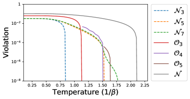
Figure 1: The strength of different PT-moment-based entanglement criteria. Here, we choose the parameters $J=1$ and $g=2.5$ for a $10$-qubit system. The entanglement for the bipartition $(1,2,\dots,5|6,7,\dots,10)$ is considered. The violations $\mathcal{N}_{n}$ and $\mathcal{O}_{n}$ are defined in Eqs. (20, 21), and $\mathcal{N}$ is the negativity of entanglement [36].

For the second example, we consider the one-dimensional quantum Ising model in a transverse magnetic field,

$$H=-J\Big{(}\sum_{i=1}^{N}\sigma_{i}^{z}\sigma_{i+1}^{z}+g\sum_{i=1}^{N}\sigma_{i}^{x}\Big{)},$$ (22)

with the periodic boundary condition ($\sigma^{z}_{N+1}=\sigma_{1}^{z}$), where $J$ corresponds to the coupling strength and $g$ is the relative strength of the external magnetic field. We study the entanglement of the thermal equilibrium (Gibbs) state $\rho(\beta)=\mathrm{e}^{-\beta H}/Z(\beta)$, where $Z(\beta)=\operatorname{Tr}[\mathrm{e}^{-\beta H}]$ is the partition function and $\beta$ is the inverse temperature. The strength of different PT-moment-based entanglement criteria for this model is illustrated in Fig. 1.

At last, we would like to note that the example in Fig. 1 also illustrates an important challenge for testing the PT-moment-based criteria. That is, the violations can become very small for higher-order criteria. Indeed, this is not specific to the PT-moments but also the other moment-based methods. The fundamental reason is that the (PT-)moments decrease exponentially as $n$ goes large. This can be easily seen from the relation that $\lvert\operatorname{Tr}(X^{n})\rvert\leq[\operatorname{Tr}(X^{2})]^{\frac{n}{2}}$ for any Hermitian operator $X$ and $n\geq 2$ . In the PT-moment problem, $\operatorname{Tr}[(\rho_{AB}^{T_{A}})^{2}]=\operatorname{Tr}[\rho_{AB}^{2}]$, which is the purity of the state. Hence, the violations in Fig. 1 become small (compared to the PPT criterion) if the temperature increases. Still, it should be remembered that a small violation is, in general, not connected to a statistically insignificant violation [41, 42, 43]; see Appendix E for more discussions. This difference also means that the numerical values of the violations in Eqs. (20, 21) should not be directly compared with each other.

Conclusion.—We have developed two systematic methods for detecting entanglement from PT-moments. The first method is based on the classical moment problems, whose lowest order gives the $p_{3}$-PPT criterion in Ref. [20] and higher orders provide strictly stronger criteria. The second method is the optimal method, which gives necessary and sufficient conditions for entanglement detection based on PT-moments. We demonstrated that our criteria are significantly better than existing criteria for physically relevant states.

For the future research, there are several possible directions. First, one may extend the presented theory by taking, instead of the transposition, other positive but not completely positive maps. This may allow one to characterize entanglement in quantum states that escape the detection by the PPT criterion. Second, for the analysis of current experiments, it would be highly desirable to extend the presented theory to the characterization of multiparticle entanglement. Indeed, potential generalizations of the PPT criterion for the multiparticle case exist [44], but how to evaluate this using randomized measurements remains an open question.

We would like to thank Andreas Ketterer, H. Chau Nguyen, Timo Simnacher, and Nikolai Wyderka for discussions. This work was supported by the Deutsche Forschungsgemeinschaft (DFG, German Research Foundation, project numbers 447948357 and 440958198), the Sino-German Center for Research Promotion, and the ERC (Consolidator Grant 683107/TempoQ).

Note added.—While finishing this manuscript, we became aware of a related work by A. Neven et al. [45].

Appendix A The moment problems

In this appendix, we show that the Hankel matrices give almost necessary and sufficient conditions for the moment problems. These results follow from well-known results in the classical moment problems, which are expressed in the language of measure theory; see, for example, Refs. [28, Chapter 3] and [29, Chapter 9]. Here, we give an elementary proof from the point of view of quantum theory. In addition, for the sufficiency part (Lemma 4 in the following), we consider the closures $\mathrm{cl}(\mathcal{M}_{n})$ and $\mathrm{cl}(\mathcal{M}_{n}^{+})$ in order to avoid the complicated rank and range conditions. We start from the proof of Lemma 1.

Lemma 1.

(a) A necessary condition for $\bm{m}^{(n)}=(m_{0},m_{1},\dots,m_{n})\in\mathcal{M}_{n}$ is that $H_{\lfloor\frac{n}{2}\rfloor}\geq 0$.
(b) A necessary condition for $\bm{m}^{(n)}=(m_{0},m_{1},\dots,m_{n})\in\mathcal{M}_{n}^{+}$ is that $H_{\lfloor\frac{n}{2}\rfloor}\geq 0$ and $B_{\lfloor\frac{n-1}{2}\rfloor}\geq 0$.

Proof.

We take advantage of the Hilbert-Schmidt inner product in the operator space

$$\langle X,Y\rangle:=\operatorname{Tr}(X^{\dagger}Y).$$ (23)

Now, consider the sequence of operators $\bm{v}=(\rho^{\frac{1}{2}},\rho^{\frac{1}{2}}X,\dots,\rho^{\frac{1}{2}}X^{\lfloor\frac{n}{2}\rfloor})$, and similarly the sequence of operators $\bm{u}=(\rho^{\frac{1}{2}}X^{\frac{1}{2}},\rho^{\frac{1}{2}}X^{\frac{3}{2}},\dots,\rho^{\frac{1}{2}}X^{\lfloor\frac{n-1}{2}\rfloor+\frac{1}{2}})$ when $X\geq 0$. Then, the Gram matrices for $\bm{v}$ and $\bm{u}$ are given by

$$\langle v_{i},v_{j}\rangle =\operatorname{Tr}(X^{i}\rho^{\frac{1}{2}}\rho^{\frac{1}{2}}X^{j})=\operatorname{Tr}(\rho X^{i+j})=m_{i+j},$$ (24)

$$\langle u_{i},u_{j}\rangle =\operatorname{Tr}(X^{i+\frac{1}{2}}\rho^{\frac{1}{2}}\rho^{\frac{1}{2}}X^{j+\frac{1}{2}})=\operatorname{Tr}(\rho X^{i+j+1})=m_{i+j+1},$$ (25)

which are just the Hankel matrices $H_{\lfloor\frac{n}{2}\rfloor}$ and $B_{\lfloor\frac{n-1}{2}\rfloor}$. As Gram matrices are always positive semidefinite [46], we get the results: (a) $H_{\lfloor\frac{n}{2}\rfloor}\geq 0$ when $\rho\geq 0$; (b) $H_{\lfloor\frac{n}{2}\rfloor}\geq 0$ and $B_{\lfloor\frac{n-1}{2}\rfloor}\geq 0$ when $\rho\geq 0$ and $X\geq 0$. ∎

Lemma 4.

(a) A necessary and sufficient condition for $\bm{m}^{(n)}=(m_{0},m_{1},\dots,m_{n})\in\mathrm{cl}(\mathcal{M}_{n})$ is that $H_{\lfloor\frac{n}{2}\rfloor}\geq 0$.
(b) A necessary and sufficient condition for $\bm{m}^{(n)}=(m_{0},m_{1},\dots,m_{n})\in\mathrm{cl}(\mathcal{M}_{n}^{+})$ is that $H_{\lfloor\frac{n}{2}\rfloor}\geq 0$ and $B_{\lfloor\frac{n-1}{2}\rfloor}\geq 0$.

Proof.

From Lemma 1, we get that the positive semidefinite property holds when $\bm{m}^{(n)}\in\mathcal{M}_{n}$ or $\bm{m}^{(n)}\in\mathcal{M}_{n}^{+}$. Then the necessity parts of both cases (a) and (b) follow from the fact that the set of positive semidefinite matrices is closed. Thus, we only need to prove the sufficiency parts.

To prove case (a), we first show that when $H_{\lfloor\frac{n}{2}\rfloor}>0$, i.e., $H_{\lfloor\frac{n}{2}\rfloor}$ is strictly positive definite, there exists $\lvert\varphi\rangle$ and $X$ of dimension $\lfloor\frac{n}{2}\rfloor+1$ such that

$$m_{k}=\operatorname{Tr}(\lvert\varphi\rangle\langle\varphi\rvert X^{k})=\langle\varphi\rvert X^{k}\lvert\varphi\rangle$$ (26)

for $k=0,1,2,\dots,n$. For simplicity, we use $\ell$ to denote $\lfloor\frac{n}{2}\rfloor$. The basic idea for proving Eq. (26) is to construct a so-called flat extension $\bm{m}^{(2\ell+2)}$ of $\bm{m}^{(n)}$, i.e., find $m_{2\ell+2}$ (choose an arbitrary $m_{2\ell+1}$ when $n$ is even) such that

$$H_{\ell+1}\geq 0,\quad\operatorname{rank}(H_{\ell+1})=\operatorname{rank}(H_{\ell}).$$ (27)

Note that $H_{\ell}>0$ implies that $\operatorname{rank}(H_{\ell})=\ell+1$. From the following decomposition

$$H_{\ell+1}=\begin{bmatrix}H_{\ell}&\bm{\mu}_{\ell}\\ \bm{\mu}_{\ell}^{T}&m_{2\ell+2}\end{bmatrix}=\begin{bmatrix}\mathds{1}&0\\ \bm{\mu}_{\ell}^{T}H_{\ell}^{-1}&1\end{bmatrix}\begin{bmatrix}H_{\ell}&0\\ 0&m_{2\ell+2}-\bm{\mu}_{\ell}^{T}H_{\ell}^{-1}\bm{\mu}_{\ell}\end{bmatrix}\begin{bmatrix}\mathds{1}&H_{\ell}^{-1}\bm{\mu}_{\ell}\\ 0&1\end{bmatrix},$$ (28)

where $\bm{\mu}_{\ell}=[m_{\ell+1},m_{\ell+2},\dots,m_{2\ell+1}]^{T}$, one can easily see that Eq. (27) is satisfied if $m_{2\ell+2}$ is chosen such that the Schur complement $m_{2\ell+2}-\bm{\mu}_{\ell}^{T}H_{\ell}^{-1}\bm{\mu}_{\ell}$ equals to zero.

From Eq. (27) and $\operatorname{rank}(H_{\ell})=\ell+1$, we can construct $\lvert\varphi_{i}\rangle\in\mathds{R}^{\ell+1}$ for $i=0,1,\dots,\ell+1$, such that

$$\langle\varphi_{i}|\varphi_{j}\rangle=[H_{\ell+1}]_{ij}=m_{i+j},$$ (29)

where $\lvert\varphi_{i}\rangle$ may not be normalized. Then, the assumption that $H_{\ell}$ is of full rank implies that $\{\lvert\varphi_{i}\rangle\mid i=0,1,\dots,\ell\}$ is a basis for $\mathds{R}^{\ell+1}$, and hence there exists a unique matrix $X\in\mathds{R}^{(\ell+1)\times(\ell+1)}$ such that

$$X\lvert\varphi_{i}\rangle=\lvert\varphi_{i+1}\rangle,\quad\text{for}~{}i=0,1,\dots,\ell.$$ (30)

From Eqs. (29, 30), we get that

$$\langle\varphi_{i}\rvert X\lvert\varphi_{j}\rangle=\langle\varphi_{j}\rvert X\lvert\varphi_{i}\rangle=m_{i+j+1}\in\mathds{R}\quad\text{for}~{}i,j=0,1,\dots,\ell,$$ (31)

which implies that the real matrix $X$ is symmetric. By letting $\lvert\varphi\rangle=\lvert\varphi_{0}\rangle$, we get that

$$X^{i}\lvert\varphi\rangle=\lvert\varphi_{i}\rangle\quad\text{for }i=0,1,\dots,\ell+1.$$ (32)

Thus, Eq. (26) follows directly from Eqs. (29, 32).

For the general case that $H_{\lfloor\frac{n}{2}\rfloor}(\bm{m})\geq 0$, we can construct a sequence of moments $\bm{m}_{s}^{(n)}$ for $s\in\mathds{N}$ such that

$$H_{\lfloor\frac{n}{2}\rfloor}(\bm{m}_{s})>0,\quad\lim_{s\to+\infty}\bm{m}_{s}^{(n)}=\bm{m}^{(n)}.$$ (33)

For example, we can take

$$\bm{m}_{s}^{(n)}=\left(1-\frac{1}{s+1}\right)\bm{m}^{(n)}+\frac{1}{s+1}\bm{m}_{0}^{(n)},$$ (34)

where $\bm{m}_{0}^{(n)}$ is an arbitrary sequence of moments such that $H_{\lfloor\frac{n}{2}\rfloor}(\bm{m}_{0})>0$, because

$$H_{\lfloor\frac{n}{2}\rfloor}(\bm{m}_{s})=\left(1-\frac{1}{s+1}\right)H_{\lfloor\frac{n}{2}\rfloor}(\bm{m})+\frac{1}{s+1}H_{\lfloor\frac{n}{2}\rfloor}(\bm{m}_{0})>0$$ (35)

for any $s\in\mathds{N}$. Then, the necessity follows directly from Eqs. (26, 33).

The proof for case (b) is similar. Again, by assuming that $H_{\lfloor\frac{n}{2}\rfloor}>0$ and $B_{\lfloor\frac{n-1}{2}\rfloor}>0$, a similar argument as in Eq. (28) implies that we can construct a flat extension $\bm{m}^{(2\lfloor\frac{n}{2}\rfloor+2)}$ of $\bm{m}^{(n)}$ such that

$$H_{\lfloor\frac{n}{2}\rfloor+1}\geq 0,\quad B_{\lfloor\frac{n}{2}\rfloor}\geq 0,\quad\operatorname{rank}\left(H_{\lfloor\frac{n}{2}\rfloor+1}\right)=\operatorname{rank}\left(H_{\lfloor\frac{n}{2}\rfloor}\right).$$ (36)

Still, we can construct $\lvert\varphi\rangle$ and $X$ as in Eqs. (29, 30), then we only need to show that $X\geq 0$. This follows from that $\{\lvert\varphi_{i}\rangle\}_{i=0}^{\ell}$ is a basis, and

$$\langle\varphi_{i}\rvert X\lvert\varphi_{j}\rangle=m_{i+j+1}=\left[B_{\ell}\right]_{ij},\quad B_{\ell}=B_{\lfloor\frac{n}{2}\rfloor}\geq 0.$$ (37)

The general case that $H_{\lfloor\frac{n}{2}\rfloor}\geq 0$ and $B_{\lfloor\frac{n-1}{2}\rfloor}\geq 0$ can be proved similarly as in Eq. (33). ∎

One may wonder whether Lemma 4 still holds without taking the closure, i.e., whether the sets $\mathcal{M}_{n}$ and $\mathcal{M}_{n}^{+}$ are closed. A well-known counterexample [28, 29] for $\mathcal{M}_{n}$ is $\bm{m}^{(4)}=(1,1,1,1,2)$ with

$$H_{2}=\begin{bmatrix}m_{0}&m_{1}&m_{2}\\ m_{1}&m_{2}&m_{3}\\ m_{2}&m_{3}&m_{4}\\ \end{bmatrix}=\begin{bmatrix}1&1&1\\ 1&1&1\\ 1&1&2\\ \end{bmatrix}\geq 0.$$ (38)

Suppose that there exists (finite- or infinite-dimensional) $\rho$ and $X$ such that $\bm{m}^{(4)}=[\operatorname{Tr}(\rho X^{k})]_{k=0}^{4}=(1,1,1,1,2)$. Then, we have that

$$\operatorname{Tr}[\rho(X-\mathds{1})^{2}]=\operatorname{Tr}[\rho^{\frac{1}{2}}(X-\mathds{1})(X-\mathds{1})\rho^{\frac{1}{2}}]=0,$$ (39)

which implies that $\rho^{\frac{1}{2}}(X-\mathds{1})=(X-\mathds{1})\rho^{\frac{1}{2}}=0$. Thus, $\rho X=\rho$ and hence $\rho X^{4}=\rho$, which is in contradiction to the fact that $\operatorname{Tr}(\rho X^{4})=m_{4}=2\operatorname{Tr}(\rho)=2m_{0}$. However, $\bm{m}^{(4)}=(1,1,1,1,2)$ can be approximated ($\varepsilon\to 0^{+}$) by

$$\rho=\begin{bmatrix}1-\varepsilon&0\\ 0&\varepsilon\end{bmatrix},\quad X=\begin{bmatrix}1&0\\ 0&\varepsilon^{-\frac{1}{4}}\end{bmatrix},$$ (40)

or equivalently, with the pure state $\lvert\varphi\rangle=\sqrt{1-\varepsilon}\lvert 0\rangle+\sqrt{\varepsilon}\lvert 1\rangle$.

For $\mathcal{M}_{n}^{+}$, we can also construct a distinct counterexample $\bm{m}^{(4)}=(1,1,2,4,9)$, which satisfies that

$$H_{2}=\begin{bmatrix}m_{0}&m_{1}&m_{2}\\ m_{1}&m_{2}&m_{3}\\ m_{2}&m_{3}&m_{4}\\ \end{bmatrix}=\begin{bmatrix}1&1&2\\ 1&2&4\\ 2&4&9\\ \end{bmatrix}>0,\quad B_{1}=\begin{bmatrix}m_{1}&m_{2}\\ m_{2}&m_{3}\\ \end{bmatrix}=\begin{bmatrix}1&2\\ 2&4\\ \end{bmatrix}\geq 0.$$ (41)

It is possible to find $\rho$ and $X$ such that $\operatorname{Tr}(\rho X^{i})=m_{i}$ according to Eq. (26). However, it is impossible to make $X\geq 0$, because

$$\operatorname{Tr}[\rho X(X-2\mathds{1})^{2}]=\operatorname{Tr}[\rho^{\frac{1}{2}}(X^{\frac{3}{2}}-2X^{\frac{1}{2}})(X^{\frac{3}{2}}-2X^{\frac{1}{2}})\rho^{\frac{1}{2}}]=0,$$ (42)

which implies that $\rho X^{2}=2\rho X$ and further $\rho X^{4}=8\rho X$. This is in contradiction to the fact that $\operatorname{Tr}(\rho X^{4})=9\operatorname{Tr}(\rho X)$. However, $\bm{m}^{(4)}=(1,1,2,4,9)$ can be approximated ($\varepsilon\to 0^{+}$) by

$$\rho=\begin{bmatrix}\frac{1}{2}&0&0\\ 0&\frac{1}{2}-\varepsilon&0\\ 0&0&\varepsilon\\ \end{bmatrix},\quad X=\begin{bmatrix}2&0&0\\ 0&0&0\\ 0&0&\varepsilon^{-\frac{1}{4}}\\ \end{bmatrix},$$ (43)

or equivalently, with the pure state $\lvert\varphi\rangle=\sqrt{1/2}\lvert 0\rangle+\sqrt{1/2-\varepsilon}\lvert 1\rangle+\sqrt{\varepsilon}\lvert 2\rangle$.

Appendix B Comparison with the higher-order criteria in Ref. [20]

In this appendix, we show that the criteria based on the Hankel matrices are strictly stronger than the criteria

$$p_{n}^{n-2}\geq p_{n-1}^{n-1},\quad\text{for}~{}n=3,4,\dots$$ (44)

which were first proposed in Ref. [20]. This fact can be proved by induction from

$$\begin{bmatrix}p_{n-2}&p_{n-1}\\ p_{n-1}&p_{n}\end{bmatrix}\geq 0,\quad\text{for}~{}n=3,4,\dots$$ (45)

which in turn follow from the positive semidefinite property of the Hankel matrices $H_{k}$ and $B_{k}$. Equation (45) implies that

$$p_{n}\geq 0,\quad p_{n}p_{n-2}\geq p_{n-1}^{2}.$$ (46)

Note that Eq. (46) gives the criterion in Eq. (44) for $n=3$, i.e., the $p_{3}$-PPT criterion. Now, assume that Eq. (44) of order $n-1$ is true, i.e., $p_{n-1}^{n-3}\geq p_{n-2}^{n-2}$, then Eq. (46) implies that

$$p_{n}^{n-2}p_{n-1}^{n-3}\geq p_{n}^{n-2}p_{n-2}^{n-2}\geq p_{n-1}^{2n-4},$$ (47)

from which Eq. (44) of order $n$ follows.

The proof also explains why the criteria in Eq. (44) are usually much weaker than the $p_{n}$-PPT criteria based on the Hankel matrices. This is because Eq. (45) only contains very limited information of the positive semidefinite property of the Hankel matrices. Especially, when $n$ is even, Eq. (45) holds for all states including the nonpositive partial transpose (NPT) ones. Indeed, the higher-order criteria in Eq. (44) are so weak that we did not find with random sampling a single instance of $\rho_{AB}$ for which they are stronger than the $p_{3}$-PPT criterion, although such states can, in principle, be constructed as follows.

The key idea is to find an NPT state $\rho_{AB}$ such that

$$p_{3}\geq p_{2}^{2},\quad\lambda_{\min}\left(\rho_{AB}^{T_{A}}\right)+\lambda_{\max}\left(\rho_{AB}^{T_{A}}\right)<0,$$ (48)

where $p_{n}=\operatorname{Tr}[(\rho_{AB}^{T_{A}})^{n}]$, and $\lambda_{\min}(\rho_{AB}^{T_{A}})$ and $\lambda_{\max}(\rho_{AB}^{T_{A}})$ are the smallest and largest eigenvalues of $\rho_{AB}^{T_{A}}$, respectively. Thus, $\rho_{AB}$ does not violate the $p_{3}$-PPT criterion, but it will violate the higher-order criterion in Eq. (44) when $n$ is a large enough odd number. This is because when $k$ is large enough

$$p_{2k+1}^{2k-1}<0<p_{2k}^{2k}.$$ (49)

Next, we show that if there exists a state $\rho_{A_{1}B_{1}}$ in $\mathcal{H}_{A_{1}}\otimes\mathcal{H}_{B_{1}}$ satisfying that

$$\lambda_{\min}\left(\rho_{A_{1}B_{1}}^{T_{A_{1}}}\right)+\lambda_{\max}\left(\rho_{A_{1}B_{1}}^{T_{A_{1}}}\right)<0,$$ (50)

then a state $\rho_{AB}$ can be constructed by adding some noise such that the first part in Eq. (48), i.e., the $p_{3}$-PPT criterion, is also satisfied. Specifically, let $\mathcal{H}_{A}\otimes\mathcal{H}_{B}=\mathcal{H}_{A_{1}A_{2}}\otimes\mathcal{H}_{B_{1}B_{2}}$ and

$$X_{AB}=\rho_{A_{1}B_{1}}\otimes\lvert 00\rangle\langle 00\rvert_{A_{2}B_{2}}+2\lambda\sum_{i=1}^{N}\lvert 00\rangle\langle 00\rvert_{A_{1}B_{1}}\otimes\lvert ii\rangle\langle ii\rvert_{A_{2}B_{2}}+\lambda\sum_{i=N+1}^{2N}\lvert 00\rangle\langle 00\rvert_{A_{1}B_{1}}\otimes\lvert ii\rangle\langle ii\rvert_{A_{2}B_{2}},$$ (51)

where $0<\lambda\leq\frac{1}{2}\lambda_{\max}(\rho_{A_{1}B_{1}}^{T_{A_{1}}})$ and $N$ is an integer to be determined, then

$$X_{AB}^{T_{A}}=\rho_{A_{1}B_{1}}^{T_{A_{1}}}\otimes\lvert 00\rangle\langle 00\rvert_{A_{2}B_{2}}+2\lambda\sum_{i=1}^{N}\lvert 00\rangle\langle 00\rvert_{A_{1}B_{1}}\otimes\lvert ii\rangle\langle ii\rvert_{A_{2}B_{2}}+\lambda\sum_{i=N+1}^{2N}\lvert 00\rangle\langle 00\rvert_{A_{1}B_{1}}\otimes\lvert ii\rangle\langle ii\rvert_{A_{2}B_{2}}.$$ (52)

Let

$$\rho_{AB}=\frac{X_{AB}}{\operatorname{Tr}(X_{AB})},$$ (53)

then it is straightforward that $\lambda_{\min}(\rho_{AB}^{T_{A}})+\lambda_{\max}(\rho_{AB}^{T_{A}})<0$ for any $N\in\mathds{N}$. Let $\tilde{p}_{n}=\operatorname{Tr}[(\rho_{A_{1}B_{1}}^{T_{A_{1}}})^{n}]$, then the $p_{3}$-PPT criterion $p_{3}\geq p_{2}^{2}$ for $\rho_{AB}$ is equivalent to that

$$\operatorname{Tr}[X_{AB}]\operatorname{Tr}[(X_{AB}^{T_{A}})^{3}]\geq\left[\operatorname{Tr}[(X_{AB}^{T_{A}})^{2}]\right]^{2}~{}\Leftrightarrow~{}2\lambda^{4}N^{2}+(9\lambda^{3}-10\tilde{p}_{2}\lambda^{2}+3\tilde{p}_{3}\lambda)N+(\tilde{p}_{3}-\tilde{p}_{2}^{2})\geq 0,$$ (54)

which can be satisfied by choosing a large enough $N$. Thus, we only need to show that there exists $\rho_{A_{1}B_{1}}$ satisfying Eq. (50). An explicit example is given by the Werner states [47]

$$\rho_{A_{1}B_{1}}=\frac{1}{d_{1}(d_{1}-1)}(\mathds{1}-V_{A_{1}A_{2}}),$$ (55)

where $V_{A_{1}B_{1}}$ is the swap operator between $\mathcal{H}_{A_{1}}$ and $\mathcal{H}_{B_{1}}$, and $d_{1}=\dim(\mathcal{H}_{A_{1}})=\dim(\mathcal{H}_{B_{1}})$. One can easily verify that

$$\lambda_{\min}\left(\rho_{A_{1}B_{1}}^{T_{A_{1}}}\right)+\lambda_{\max}\left(\rho_{A_{1}B_{1}}^{T_{A_{1}}}\right)=-\frac{(d_{1}-2)}{d_{1}(d_{1}-1)},$$ (56)

which is always negative when $d_{1}\geq 3$.

Appendix C The optimal method for the PT-moment problem

In this appendix, we describe in detail the optimal method for the PT-moment problem. As explained in the main text, this is equivalent to characterizing the difference between

$$\mathcal{T}_{n}^{+} ={\Big{\{}\bm{p}^{(n)}=(p_{0},p_{1},\dots,p_{n})\,\Big{|}\,\sum_{i=1}^{d}x_{i}^{k}=p_{k},~{}x_{i}\geq 0\Big{\}}},$$ (57)

$$\mathcal{T}_{n} ={\Big{\{}\bm{p}^{(n)}=(p_{0},p_{1},\dots,p_{n})\,\Big{|}\,\sum_{i=1}^{d}x_{i}^{k}=p_{k},~{}x_{i}\in\mathds{R}\Big{\}}}.$$ (58)

To this end, we consider the following optimization problems,

$$\underset{x_{i}}{\mathrm{min}}/\underset{x_{i}}{\mathrm{max}}\quad \hat{p}_{n}:=\sum_{i=1}^{d}x_{i}^{n}$$ (59)

$$\mathrm{subject~{}to} \sum_{i=1}^{d}x_{i}^{k}=p_{k}\quad~{}\text{for}~{}k=1,2,\dots,n-1,$$

$$x_{1}\geq x_{2}\geq\dots\geq x_{d}\geq 0.$$

Then, the moment $p_{n}$ should be within $[\hat{p}_{n}^{\min},\hat{p}_{n}^{\max}]$, which gives a necessary condition for the moments to originate from a separable state. Actually, as shown in the following, this condition is also sufficient as there is no local minimum and maximum apart from the global ones. We start from the case that $n=3$ and prove Theorem 3 from the main text.

Theorem 3.

(a) There exists a $d$-dimensional separable (PPT) state $\rho_{AB}$ satisfying that $p_{k}=\operatorname{Tr}[(\rho^{T_{A}}_{AB})^{k}]$ for $k=1,2,3$, if and only if

$$p_{1}=1,\quad\frac{1}{d}\leq p_{2}\leq 1,\quad\alpha x^{3}+(1-\alpha x)^{3}\leq p_{3}\leq[1-(d-1)y]^{3}+(d-1)y^{3},$$ (60)

where $\alpha=\lfloor\frac{1}{p_{2}}\rfloor$, $x=\frac{\alpha+\sqrt{\alpha[p_{2}(\alpha+1)-1]}}{\alpha(\alpha+1)}$, and $y=\frac{d-1-\sqrt{(d-1)(p_{2}d-1)}}{d(d-1)}$.
(b) More importantly, suppose that the $p_{k}$ for $k=1,2,3$ are PT-moments from a quantum state. Then, they are compatible with a separable (PPT) state if and only if

$$p_{3}\geq\alpha x^{3}+(1-\alpha x)^{3},$$ (61)

where $\alpha$ and $x$ are as above.

Proof.

It is well-known that $p_{1}=\operatorname{Tr}[\rho_{AB}^{T_{A}}]=\operatorname{Tr}[\rho_{AB}]=1$, and further the optimization problems in Eq. (59) for $n=3$ are feasible if and only if $1/d\leq p_{2}\leq 1$. To solve the optimization problems in Eq. (59) for $n=3$, we start from the simplest nontrivial case that $d=3$. Then, the optimization reads

$$\underset{x_{i}}{\mathrm{min}}/\underset{x_{i}}{\mathrm{max}}\quad \hat{p}_{3}:=x_{1}^{3}+x_{2}^{3}+x_{3}^{3}$$ (62)

$$\mathrm{subject~{}to} x_{1}+x_{2}+x_{3}=p_{1},$$

$$x_{1}^{2}+x_{2}^{2}+x_{3}^{2}=p_{2},$$

$$x_{1}\geq x_{2}\geq x_{3}\geq 0,$$

where $p_{1}$ and $p_{2}$ are constants and $\hat{p}_{3}$ is the objective function that we want to optimize. From Eq. (62) we can get how $\hat{p}_{3}$ varies with $x_{i}$, i.e., the relations between the differentials $\mathrm{d}\hat{p}_{3}$ and $\mathrm{d}x_{i}$,

$$\mathrm{d}x_{1}+\hbox{} \mathrm{d}x_{2}+\hbox{} \mathrm{d}x_{3} =0,$$ (63)

$$x_{1} \mathrm{d}x_{1}+x_{2} \mathrm{d}x_{2}+x_{3} \mathrm{d}x_{3} =0,$$

$$x_{1}^{2} \mathrm{d}x_{1}+x_{2}^{2} \mathrm{d}x_{2}+x_{3}^{2} \mathrm{d}x_{3} =\frac{1}{3}\mathrm{d}\hat{p}_{3}.$$

This can be viewed as a system of linear equations on $\mathrm{d}x_{i}$ and can be directly solved by taking advantage of Cramer’s rule and the Vandermonde determinant [46], whenever $x_{i}$ are all different. This gives the following relations between $\mathrm{d}\hat{p}_{3}$ and $\mathrm{d}x_{i}$

$$\mathrm{d}\hat{p}_{3}= 3(x_{1}-x_{2})(x_{1}-x_{3})\mathrm{d}x_{1}$$ (64)

$$= 3(x_{2}-x_{3})(x_{2}-x_{1})\mathrm{d}x_{2}$$

$$= 3(x_{3}-x_{1})(x_{3}-x_{2})\mathrm{d}x_{3}.$$

Recalling that $x_{1}\geq x_{2}\geq x_{3}$ by assumption, Eq. (64) implies that $\mathrm{d}x_{i}$ are not independent and an alternating relation exists between them. For example, $\mathrm{d}x_{1}>0$ will result in that $\mathrm{d}x_{2}<0$ and $\mathrm{d}x_{3}>0$ (when $x_{i}$ are all different). Further, Eq. (64) also implies that if the optimization problems in Eq. (62) are feasible, then $\mathrm{d}\hat{p}_{3}>0$ when $x_{1}$ increases (and thus $x_{2}$ decreases and $x_{3}$ increases); and $\mathrm{d}\hat{p}_{3}<0$ when $x_{1}$ decreases (and thus $x_{2}$ increases and $x_{3}$ decreases). Then, without the boundary condition $x_{i}\geq 0$, the maximum of $\hat{p}_{3}$ will be achieved when $x_{2}=x_{3}$ and the minimum will be achieved when $x_{1}=x_{2}$. When the boundary condition $x_{3}\geq 0$ is taken into consideration, the minimum may also be achieved when $x_{3}$ decreases to zero.

Note that the above analysis does not depend on the actual values of $p_{1}$ and $p_{2}$ (even if $p_{1}\neq 1$). This implies that if the optimization problems in Eq. (11) for $\hat{p}_{3}$ ($n=3$) are feasible, the (local) maximum will be achieved only if

$$\bm{x}_{3}^{\max}=(x_{1},\underbrace{x_{2},x_{2},\dots,x_{2}}_{d-1~{}\text{times}}),$$ (65)

and the (local) minimum will be achieved only if

$$\bm{x}_{3}^{\min}=(\underbrace{x_{1},x_{1},\cdots,x_{1}}_{\alpha~{}\text{times}},x_{\alpha+1},\underbrace{0,0,\dots,0}_{d-\alpha-1~{}\text{times}}).$$ (66)

This is because for the maximization any tuple $(x_{i_{1}},x_{i_{2}},x_{i_{3}})$ with $i_{1}<i_{2}<i_{3}$ needs to satisfy that $x_{i_{2}}=x_{i_{3}}$, and for the minimization it needs to satisfy that $x_{i_{1}}=x_{i_{2}}$ or $x_{i_{3}}=0$. Without loss of generality, we assume that $x_{\alpha+1}\neq x_{1}$ in Eq. (66), then the integer $\alpha$ is uniquely determined by

$$\alpha=\left\lfloor\frac{1}{p_{2}}\right\rfloor.$$ (67)

This is because the majorization relation

$$\Big{(}\underbrace{\frac{1}{\alpha+1},\frac{1}{\alpha+1},\dots,\frac{1}{\alpha+1}}_{\alpha+1~{}\text{times}},\underbrace{\vphantom{\frac{1}{\alpha+1}}0,0,\dots,0}_{d-\alpha-1~{}\text{times}}\Big{)}\prec(\underbrace{x_{1},x_{1},\cdots,x_{1}}_{\alpha~{}\text{times}},x_{\alpha+1},\underbrace{0,0,\dots,0}_{d-\alpha-1~{}\text{times}})\prec\Big{(}\underbrace{\frac{1}{\alpha},\frac{1}{\alpha},\dots,\frac{1}{\alpha}}_{\alpha~{}\text{times}},\underbrace{\vphantom{\frac{1}{\alpha}}0,0,\dots,0}_{d-\alpha~{}\text{times}}\Big{)}.$$ (68)

and the strict Schur-convexity of $p_{2}=\sum_{i=1}^{d}x_{i}^{2}$ [48] imply that $1/(\alpha+1)<p_{2}\leq 1/\alpha$.

Now, from Eq. (65), we can get that

$$x_{1}+(d-1)x_{2}=1,$$ (69)

$$x_{1}^{2}+(d-1)x_{2}^{2}=p_{2},$$

$$x_{1}\geq x_{2}\geq 0.$$

Given the feasibility condition $1/d\leq p_{2}\leq 1$, Eq. (69) has a unique solution

$$x_{1}=\frac{\sqrt{(d-1)(p_{2}d-1)}+1}{d},\quad x_{2}=\frac{d-1-\sqrt{(d-1)(p_{2}d-1)}}{d(d-1)}.$$ (70)

From Eq. (66), we can get that

$$\alpha x_{1}+x_{\alpha+1}=1,$$ (71)

$$\alpha x_{1}+x_{\alpha+1}^{2}=p_{2},$$

$$x_{1}\geq x_{\alpha+1}\geq 0,$$

which also has a unique solution

$$x_{1}=\frac{\alpha+\sqrt{\alpha[p_{2}(\alpha+1)-1]}}{\alpha(\alpha+1)},\quad x_{\alpha+1}=\frac{1-\sqrt{\alpha[p_{2}(\alpha+1)-1]}}{\alpha+1}.$$ (72)

So far, we only considered the conditions for local extrema, and found that the minimum and maximum are unique as in Eqs. (70, 72). This implies that these are the global extrema. Further, the uniqueness of the extrema and the continuity of $\hat{p}_{3}$ also imply that the closed feasible region is connected. Thus, all values between the minimum and the maximum are achievable. All these arguments lead to the optimal result in Theorem 3(a).

For Theorem 3(b), as $p_{1}=\operatorname{Tr}[\rho_{AB}^{T_{A}}]=\operatorname{Tr}[\rho_{AB}]$ and $p_{2}=\operatorname{Tr}[(\rho_{AB}^{T_{A}})^{2}]=\operatorname{Tr}[\rho_{AB}^{2}]$, the conditions that $p_{1}=1$ and $1/d\leq p_{2}\leq 1$ are always satisfied by all (separable or entangled) states. To show the redundancy of $p_{3}\leq\hat{p}_{3}^{\max}$, we need to consider the optimization problems in Eq. (59) without the positivity constraints $x_{i}\geq 0$. From Eq. (64), we can see that the maximization is still achieved when $\bm{x}$ is of the form in Eq. (65). Given the above conditions $p_{1}=1$ and $1/d\leq p_{2}\leq 1$, the solution is always positive from Eq. (70). Thus, we prove the optimal result in Theorem 3(b). ∎

We note that for the case $n=3$ the bounds in Theorem 3(a) can also be derived from the optimization of Rényi/Tsallis entropy [49], but our method has the advantages that the refined result in Theorem 3(b) is given, and more importantly, it can be directly generalized to higher-order optimizations in Eq. (59). We take $n=4$ as an example to illustrate this. The basic idea is still to consider the simplest nontrivial situation that $d=4$ first, i.e.,

$$\underset{x_{i}}{\mathrm{min}}/\underset{x_{i}}{\mathrm{max}}\quad \hat{p}_{4}:=x_{1}^{4}+x_{2}^{4}+x_{3}^{4}+x_{4}^{4}$$ (73)

$$\mathrm{subject~{}to} x_{1}+x_{2}+x_{3}+x_{4}=p_{1},$$

$$x_{1}^{2}+x_{2}^{2}+x_{3}^{2}+x_{4}^{2}=p_{2},$$

$$x_{1}^{3}+x_{2}^{3}+x_{3}^{3}+x_{4}^{3}=p_{3},$$

$$x_{1}\geq x_{2}\geq x_{3}\geq x_{4}\geq 0,$$

for which an analog of Eq. (63) reads

$$\mathrm{d}x_{1}+\hbox{} \mathrm{d}x_{2}+\hbox{} \mathrm{d}x_{3}+\hbox{} \mathrm{d}x_{4} =0,$$ (74)

$$x_{1} \mathrm{d}x_{1}+x_{2} \mathrm{d}x_{2}+x_{3} \mathrm{d}x_{3}+x_{4} \mathrm{d}x_{4} =0,$$

$$x_{1}^{2} \mathrm{d}x_{1}+x_{2}^{2} \mathrm{d}x_{2}+x_{3}^{2} \mathrm{d}x_{3}+x_{4}^{2} \mathrm{d}x_{4} =0,$$

$$x_{1}^{3} \mathrm{d}x_{1}+x_{2}^{3} \mathrm{d}x_{2}+x_{3}^{3} \mathrm{d}x_{3}+x_{4}^{3} \mathrm{d}x_{4} =\frac{1}{4}\mathrm{d}\hat{p}_{4}.$$

Then, Cramer’s rule and the Vandermonde determinant imply

$$\mathrm{d}\hat{p}_{4}= 4(x_{1}-x_{2})(x_{1}-x_{3})(x_{1}-x_{4})\mathrm{d}x_{1}$$ (75)

$$= 4(x_{2}-x_{3})(x_{2}-x_{4})(x_{2}-x_{1})\mathrm{d}x_{2}$$

$$= 4(x_{3}-x_{4})(x_{3}-x_{1})(x_{3}-x_{2})\mathrm{d}x_{3}$$

$$= 4(x_{4}-x_{1})(x_{4}-x_{2})(x_{4}-x_{3})\mathrm{d}x_{4}.$$

With a similar argument as for Eq. (64), we get that when the optimization problems in Eq. (73) are feasible, the maximum is achieved when $x_{2}=x_{3}$ or $x_{4}=0$, and the minimum is achieved when $x_{1}=x_{2}$ or $x_{3}=x_{4}$. This analysis implies that if the optimization problems in Eq. (11) for $\hat{p}_{4}$ are feasible i.e., all the conditions in Theorem 3(a) are satisfied, the maximum will be achieved only if

$$\bm{x}_{4}^{\max}=(x_{1},\underbrace{x_{2},x_{2},\dots,x_{2}}_{\beta~{}\text{times}},x_{\beta+2},\underbrace{0,0,\dots,0}_{d-\beta-2~{}\text{times}}),$$ (76)

and the minimum will be achieved only if

$$\bm{x}_{4}^{\min}=(\underbrace{x_{1},x_{1}\cdots,x_{1}}_{\gamma~{}\text{times}},x_{\gamma+1},\underbrace{x_{\gamma+2},x_{\gamma+2},\dots,x_{\gamma+2}}_{d-\gamma-1~{}\text{times}}).$$ (77)

Furthermore, the vectors $\bm{x}_{4}^{\max}$ and $\bm{x}_{4}^{\min}$ are uniquely determined. The argument for the uniqueness is easy but tedious. Here, we only take $\bm{x}_{4}^{\max}$ as an example to show the basic idea; the uniqueness of $\bm{x}_{4}^{\min}$ can be proved similarly. The task is to prove that the equations

$$x_{1}+\beta x_{2}+x_{\beta+2}=1,$$ (78)

$$x_{1}^{2}+\beta x_{2}^{2}+x_{\beta+2}^{2}=p_{2},$$

$$x_{1}^{3}+\beta x_{2}^{3}+x_{\beta+2}^{3}=p_{3},$$

$$x_{1}\geq x_{2}\geq x_{\beta+2}\geq 0.$$

uniquely determine $\beta,x_{1},x_{2},x_{\beta+2}$. To this end, we fix $p_{2}$ but treat $p_{3}$ as a function on $\beta,x_{1},x_{2},x_{\beta+2}$. We aim to show that that $p_{3}$ is monotonically increasing on $x_{1}$ (for fixed $p_{2}$) and thus $p_{2},p_{3}$ uniquely determine $x_{1}$. Then, as in Eq. (66), for fixed $p_{2}$ and $x_{1}$, the equations

$$\beta x_{2}+x_{\beta+2}=1-x_{1},$$ (79)

$$\beta x_{2}^{2}+x_{\beta+2}^{2}=p_{2}-x^{2}_{1},$$

uniquely determine $\beta$, $x_{2}$, and $x_{\beta+2}$ and hence, given the feasibility, $\bm{x}_{4}^{\max}$ is uniquely determined by $p_{2}$ and $p_{3}$.

In the following, we always assume that $p_{2}$ is fixed. Similarly to Eq. (64), we can show that for fixed $\beta$, $\mathrm{d}p_{3}>0$ if $\mathrm{d}x_{1}>0$. Then, we only need to show that there is no overlap between the ranges of $p_{3}$ for different $\beta$ (except the extrema). To this end, we apply a similar argument as in Eqs. (62, 63, 64) to the following optimization for fixed $\beta$,

$$\underset{x_{i}}{\mathrm{min}}/\underset{x_{i}}{\mathrm{max}}\quad p_{3}:=x_{1}^{3}+\beta x_{2}^{3}+x_{\beta+2}^{3}$$ (80)

$$\mathrm{subject~{}to} x_{1}+\beta x_{2}+x_{\beta+2}=1,$$

$$x_{1}^{2}+\beta x_{2}^{2}+x_{\beta+2}^{2}=p_{2},$$

$$x_{1}\geq x_{2}\geq x_{\beta+2}\geq 0.$$

One can show that the minimization is achieved when $x_{1}=x_{2}$ or $x_{\beta+2}=0$, and the maximization is achieved when $x_{2}=x_{\beta+2}$. When these optimization results are written down consecutively for all possible $\beta$, i.e., from $\beta=\alpha-1=\lfloor 1/p_{2}\rfloor-1$ to $\beta=d-2$, one can easily see that $p_{3}$ is monotonically increasing in following process ($\nearrow$ denotes increasing and $\searrow$ denotes decreasing)

$$(x_{1}^{\nearrow},\underbrace{x_{1}^{\searrow},x_{1}^{\searrow},\dots,x_{1}^{\searrow}}_{\alpha-1~{}\text{times}},x_{\alpha+1}^{\nearrow},\underbrace{0,0,\dots,0}_{d-\alpha-1~{}\text{times}}) \Rightarrow{}{} (x_{1}^{\nearrow},\underbrace{x_{2}^{\searrow},x_{2}^{\searrow},\dots,x_{2}^{\searrow}}_{\alpha-1~{}\text{times}},x_{\alpha+1}^{\nearrow},\underbrace{0,0,\dots,0}_{d-\alpha-1~{}\text{times}})$$ (81)

$$\Rightarrow{} (x_{1}^{\nearrow},\underbrace{x_{2}^{\searrow},x_{2}^{\searrow},\dots,x_{2}^{\searrow}}_{\alpha~{}\text{times}},0^{\nearrow},\underbrace{0,0,\dots,0}_{d-\alpha-2~{}\text{times}}) \Rightarrow{}{} (x_{1}^{\nearrow},\underbrace{x_{2}^{\searrow},x_{2}^{\searrow},\dots,x_{2}^{\searrow}}_{\alpha~{}\text{times}},x_{\alpha+2}^{\nearrow},\underbrace{0,0,\dots,0}_{d-\alpha-2~{}\text{times}})$$

$$\vdots$$

$$\Rightarrow{} (x_{1}^{\nearrow},\underbrace{x_{2}^{\searrow},x_{2}^{\searrow},\dots,x_{2}^{\searrow}}_{\beta~{}\text{times}},0^{\nearrow},\underbrace{0,0,\dots,0}_{d-\beta-2~{}\text{times}}) \Rightarrow{}{} (x_{1}^{\nearrow},\underbrace{x_{2}^{\searrow},x_{2}^{\searrow},\dots,x_{2}^{\searrow}}_{\beta~{}\text{times}},x_{\beta+2}^{\nearrow},\underbrace{0,0,\dots,0}_{d-\beta-2~{}\text{times}})$$

$$\Rightarrow{} (x_{1}^{\nearrow},\underbrace{x_{2}^{\searrow},x_{2}^{\searrow},\dots,x_{2}^{\searrow}}_{\beta+1~{}\text{times}},0^{\nearrow},\underbrace{0,0,\dots,0}_{d-\beta-3~{}\text{times}}) \Rightarrow{}{} (x_{1}^{\nearrow},\underbrace{x_{2}^{\searrow},x_{2}^{\searrow},\dots,x_{2}^{\searrow}}_{\beta+1~{}\text{times}},x_{\beta+3}^{\nearrow},\underbrace{0,0,\dots,0}_{d-\beta-3~{}\text{times}})$$

$$\vdots$$

$$\Rightarrow{} (x_{1}^{\nearrow},\underbrace{x_{2}^{\searrow},x_{2}^{\searrow},\dots,x_{2}^{\searrow}}_{d-2~{}\text{times}},x_{d}^{\nearrow}) \Rightarrow{}{} (x_{1},\underbrace{x_{2},x_{2},\dots,x_{2}}_{d-1~{}\text{times}}).$$

Thus, $p_{3}$ is monotonically increasing on $x_{1}$ and there is no overlap between the ranges of $p_{3}$ for different $\beta$ (except the extrema)

The above arguments also provide a method to determine $\beta$ and then $\bm{x}_{4}^{\max}$ completely. Let $\beta_{0}$ be the unique solution of the following equations

$$x_{1}+\beta_{0}x_{2}=1,$$ (82)

$$x_{1}^{2}+\beta_{0}x_{2}^{2}=p_{2},$$

$$x_{1}^{3}+\beta_{0}x_{2}^{3}=p_{3},$$

$$x_{1}\geq x_{2}\geq 0,~{}\beta_{0}\geq 1,$$

then $\beta=\lfloor\beta_{0}\rfloor$ and the maximum point $\bm{x}_{4}^{\max}$ in Eq. (76) can be obtained by solving Eq. (78).

Similarly, let $\gamma_{0}$ be the unique solution of the following equations (unless $p_{k}=1/d^{k-1}$)

$$\gamma_{0}x_{1}+(d-\gamma_{0})x_{2}=1,$$ (83)

$$\gamma_{0}x_{1}^{2}+(d-\gamma_{0})x_{2}^{2}=p_{2},$$

$$\gamma_{0}x_{1}^{3}+(d-\gamma_{0})x_{2}^{3}=p_{3},$$

$$x_{1}\geq x_{2}\geq 0,~{}\gamma_{0}\geq 1.$$

then $\gamma=\lfloor\gamma_{0}\rfloor$ and minimum point $\bm{x}_{4}^{\min}$ in Eq. (77) can be obtained by solving

$$\gamma x_{1}+x_{\gamma+1}+(d-\gamma-1)x_{\gamma+2}=1,$$ (84)

$$\gamma x_{1}^{2}+x_{\gamma+1}^{2}+(d-\gamma-1)x_{\gamma+2}^{2}=p_{2},$$

$$\gamma x_{1}^{3}+x_{\gamma+1}^{3}+(d-\gamma-1)x_{\gamma+2}^{3}=p_{3},$$

$$x_{1}\geq x_{\gamma+1}\geq x_{\gamma+2}\geq 0.$$

Thus, given the feasibility, i.e., all the conditions in Theorem 3(a) are satisfied, the necessary and sufficient condition for $\rho_{AB}$ can be separable (PPT) is

$$\hat{p}_{4}^{\min}\leq p_{4}\leq\hat{p}_{4}^{\max},$$ (85)

where $\hat{p}_{4}^{\min}$ and $\hat{p}_{4}^{\max}$ are determined by $\bm{x}_{4}^{\min}$ in Eq. (77) and $\bm{x}_{4}^{\max}$ in Eq. (76), respectively. Correspondingly, we can show that the lower bound is redundant because $\bm{x}_{4}^{\min}$ is also the minimum without the positivity constraints $x_{i}\geq 0$. An intuitive way to understand why $\bm{x}_{3}^{\max}$ and $\bm{x}_{4}^{\min}$ are redundant is that they are extrema that are not on the boundary of nonnegative vectors.

With an analogous procedure, we can also solve the optimization problems in Eq. (59) for $n=5$, where the maximum will be achieved only if

$$\bm{x}_{5}^{\max}=(x_{1},\underbrace{x_{2},x_{2},\dots,x_{2}}_{\kappa~{}\text{times}},x_{\kappa+2},\underbrace{x_{\kappa+3},x_{\kappa+3},\dots,x_{\kappa+3}}_{d-\kappa-2~{}\text{times}}),$$ (86)

and the minimum will be achieved only if

$$\bm{x}_{5}^{\min}=(\underbrace{x_{1},x_{1},\cdots,x_{1}}_{\eta~{}\text{times}},x_{\eta+1},\underbrace{x_{\eta+2},x_{\eta+2}\dots,x_{\eta+2}}_{\xi~{}\text{times}},x_{\eta+\xi+2},\underbrace{0,0,\dots,0}_{d-\eta-\xi-2~{}\text{times}}).$$ (87)

In this case, it is more complicated to determine $\bm{x}^{\max}_{5}$ and $\bm{x}^{\min}_{5}$. Instead of writing down the complicated formula, we provide the Mathematica code for performing the optimizations.

Appendix D Additional numerical results

Figure 2: An illustration of the difference between the optimal criterion $p_{3}$-OPPT in Theorem 3(b) and the $p_{3}$-PPT condition $p_{3}\geq p_{2}^{2}$ in Ref. [20]. This shows that the violation of the optimal criterion can be up to $12.5\%$ larger.

$D$	NPT	NPT$3$	ONPT$3$	ONPT$4$	NPT$5$
10	100%	19.54%	29.74%	100%	100%
20	100%	18.81%	29.10%	100%	100%
30	100%	18.51%	28.83%	100%	100%
40	100%	18.50%	28.92%	100%	100%

Table 2: Fraction of (large) $D\times D$ states in the Hilbert-Schmidt distribution (100,000 samples) that can be detected with the various criteria. Here, NPT denotes the states violating the PPT criterion, NPT$n$ (NPT$3$, NPT$5$) denote the states violating the $p_{n}$-PPT criterion in Eq. (8), and ONPT$n$ (ONPT$3$, ONPT$4$) denote the states violating the $p_{n}$-OPPT criterion. Note that in Tables 1 and 2, the difference between $100\%$ and $100.00\%$ is that the former is an exact value, while the latter is an approximate value. In addition, see Ref. [50] for an asymptotic behavior ($D\to+\infty$) of the moments for all PPT states.

Appendix E Statistical analysis

In Refs. [20, 22], it was already shown that the PT-moments $p_{n}=\operatorname{Tr}[(\rho_{AB}^{T_{A}})^{n}]$ can be efficiently measured with the classical shadows and $U$-statistics. The statistical error is also explicitly analyzed for $n\leq 3$. The extension the higher-order case is straightforward but tedious. To obtain a general result for arbitrary $n$, we focus on the high accuracy limit (i.e., the error $\varepsilon\ll 1$), and show that for any $N$-qubit state and an arbitrary bipartition $(A|B)$, a total of

$$M\sim\frac{n^{2}2^{N}p_{2}^{n-1}}{\varepsilon^{2}\delta}$$ (88)

copies of the state suffice to ensure that the estimated $\hat{p}_{n}$ obeys $\lvert\hat{p}_{n}-p_{n}\rvert\leq\varepsilon$ with probability at least $1-\delta$. The $n^{2}p_{2}^{n-1}$ scaling in Eq. (88) implies that measuring the higher-order PT-moments does not take many more measurements compared to the lower-order ones; moreover, it also shows that for fixed $N,n,\delta$ the error $\varepsilon$ is proportional to $p_{2}^{(n-1)/2}$. This property is very important for tackling the problem that higher-order PT-moments decrease exponentially, i.e., $p_{n}\leq p_{2}^{n/2}$ discussed in the main text.

Equation (88) follows directly from the statistical analysis in Appendix D of Ref. [20]. For simplicity, we do not restate the data acquisition and processing protocol, but refer the readers to Ref. [20, 22] for the details of the classical shadow formalism. Also, we employ similar notations to make the proof easier to follow. Similarly to Eqs. (D16, D22) in Ref. [20], one can easily show that the variance of the estimator $\hat{p}_{n}$ reads

$$\operatorname{Var}(\hat{p}_{n})= {\binom{M}{n}}^{-1}\binom{n}{1}\binom{M-n}{n-1}\operatorname{Var}\left[\operatorname{Tr}\left(\left(\rho_{AB}^{T_{A}}\right)^{n-1}\hat{\rho}_{AB}^{T_{A}}\right)\right]+\mathcal{O}\left(\frac{1}{M^{2}}\right)$$ (89)

$$\leq \frac{n^{2}}{M}L+\mathcal{O}\left(\frac{1}{M^{2}}\right),$$ (90)

where $L$ denotes the linear contribution

$$L=\operatorname{Var}\left[\operatorname{Tr}\left(\left(\rho_{AB}^{T_{A}}\right)^{n-1}\hat{\rho}_{AB}^{T_{A}}\right)\right],$$ (91)

and its coefficient results from

$$\frac{\binom{n}{1}\binom{M-n}{n-1}}{\binom{M}{n}}=\frac{\binom{n}{1}\binom{M-n}{n-1}}{\frac{M}{n}\binom{M-1}{n-1}}\leq\frac{\binom{n}{1}}{\frac{M}{n}}=\frac{n^{2}}{M}.$$ (92)

The high accuracy limit $\varepsilon\ll 1$ also implies that $M\gg 1$, thus we can ignore the higher-order terms in Eq. (90). To estimate the linear contribution $L$, we set

$$O=\left(\rho_{AB}^{T_{A}}\right)^{n-1},$$ (93)

then

$$L=\operatorname{Var}\left[\operatorname{Tr}\left(O\hat{\rho}_{AB}^{T_{A}}\right)\right]=\operatorname{Var}\left[\operatorname{Tr}\left(O^{T_{A}}\hat{\rho}_{AB}\right)\right]\leq 2^{N}\operatorname{Tr}\big{[}(O^{T_{A}})^{2}\big{]},$$ (94)

where the inequality follows from Eq. (D7) in Ref. [20]. Further,

$$\operatorname{Tr}\big{[}(O^{T_{A}})^{2}\big{]}=\operatorname{Tr}\big{[}O^{2}\big{]}=\operatorname{Tr}\left[(\rho_{AB}^{T_{A}})^{2(n-1)}\right]\leq\left[\operatorname{Tr}\big{[}(\rho_{AB}^{T_{A}})^{2}\big{]}\right]^{n-1}=p_{2}^{n-1},$$ (95)

where we have used the relation that $\operatorname{Tr}(X^{n-1})\leq[\operatorname{Tr}(X)]^{n-1}$ for any $X\geq 0$. Thus, we get that

$$\operatorname{Var}(\hat{p}_{n})\leq\frac{n^{2}2^{N}p_{2}^{n-1}}{M}+\mathcal{O}\left(\frac{1}{M^{2}}\right).$$ (96)

Then, Eq. (88) follows directly from the Chebyshev inequality

$$P\big{(}\lvert\hat{p}_{n}-p_{n}\rvert\geq\varepsilon\big{)}\leq\frac{\operatorname{Var}(\hat{p}_{n})}{\varepsilon^{2}}.$$ (97)

References

• Preskill [2018] J. Preskill, Quantum computing in the NISQ era and beyond, Quantum 2, 79 (2018).
• Paris and Řeháček [2004] M. Paris and J. Řeháček, eds., Quantum State Estimation, Lecture Notes in Physics, Vol. 649 (Springer, Heidelberg, 2004).
• Eisert et al. [2020] J. Eisert, D. Hangleiter, N. Walk, I. Roth, D. Markham, R. Parekh, U. Chabaud, and E. Kashefi, Quantum certification and benchmarking, Nat. Rev. Phys. 2, 382 (2020).
• Kliesch and Roth [2021] M. Kliesch and I. Roth, Theory of quantum system certification, PRX Quantum 2, 010201 (2021).
• Horodecki et al. [2009] R. Horodecki, P. Horodecki, M. Horodecki, and K. Horodecki, Quantum entanglement, Rev. Mod. Phys. 81, 865 (2009).
• Gühne and Tóth [2009] O. Gühne and G. Tóth, Entanglement detection, Phys. Rep. 474, 1 (2009).
• Friis et al. [2019] N. Friis, G. Vitagliano, M. Malik, and M. Huber, Entanglement certification from theory to experiment, Nat. Rev. Phys. 1, 72 (2019).
• Tran et al. [2015] M. C. Tran, B. Dakić, F. Arnault, W. Laskowski, and T. Paterek, Quantum entanglement from random measurements, Phys. Rev. A 92, 050301(R) (2015).
• Tran et al. [2016] M. C. Tran, B. Dakić, W. Laskowski, and T. Paterek, Correlations between outcomes of random measurements, Phys. Rev. A 94, 042302 (2016).
• van Enk and Beenakker [2012] S. J. van Enk and C. W. J. Beenakker, Measuring $\mathrm{Tr}{\rho}^{n}$ on single copies of $\rho$ using random measurements, Phys. Rev. Lett. 108, 110503 (2012).
• Elben et al. [2019] A. Elben, B. Vermersch, C. F. Roos, and P. Zoller, Statistical correlations between locally randomized measurements: A toolbox for probing entanglement in many-body quantum states, Phys. Rev. A 99, 052323 (2019).
• Brydges et al. [2019] T. Brydges, A. Elben, P. Jurcevic, B. Vermersch, C. Maier, B. P. Lanyon, P. Zoller, R. Blatt, and C. F. Roos, Probing rényi entanglement entropy via randomized measurements, Science 364, 260 (2019).
• Ketterer et al. [2019] A. Ketterer, N. Wyderka, and O. Gühne, Characterizing multipartite entanglement with moments of random correlations, Phys. Rev. Lett. 122, 120505 (2019).
• Ketterer et al. [2020] A. Ketterer, N. Wyderka, and O. Gühne, Entanglement characterization using quantum designs, Quantum 4, 325 (2020).
• [15] A. Ketterer, S. Imai, N. Wyderka, and O. Gühne, Certifying multiparticle entanglement with randomized measurements, arXiv:2012.12176 .
• Knips et al. [2020] L. Knips, J. Dziewior, W. Kłobus, W. Laskowski, T. Paterek, P. J. Shadbolt, H. Weinfurter, and J. D. A. Meinecke, Multipartite entanglement analysis from random correlations, npj Quantum Inf. 6, 51 (2020).
• Imai et al. [2021] S. Imai, N. Wyderka, A. Ketterer, and O. Gühne, Bound entanglement from randomized measurements, Phys. Rev. Lett. 126, 150501 (2021).
• Peres [1996] A. Peres, Separability criterion for density matrices, Phys. Rev. Lett. 77, 1413 (1996).
• Gray et al. [2018] J. Gray, L. Banchi, A. Bayat, and S. Bose, Machine-learning-assisted many-body entanglement measurement, Phys. Rev. Lett. 121, 150503 (2018).
• Elben et al. [2020] A. Elben, R. Kueng, H.-Y. R. Huang, R. van Bijnen, C. Kokail, M. Dalmonte, P. Calabrese, B. Kraus, J. Preskill, P. Zoller, and B. Vermersch, Mixed-state entanglement from local randomized measurements, Phys. Rev. Lett. 125, 200501 (2020).
• Zhou et al. [2020] Y. Zhou, P. Zeng, and Z. Liu, Single-copies estimation of entanglement negativity, Phys. Rev. Lett. 125, 200502 (2020).
• Huang et al. [2020] H.-Y. Huang, R. Kueng, and J. Preskill, Predicting many properties of a quantum system from very few measurements, Nat. Phys. 16, 1050 (2020).
• Ekert et al. [2002] A. K. Ekert, C. M. Alves, D. K. L. Oi, M. Horodecki, P. Horodecki, and L. C. Kwek, Direct estimations of linear and nonlinear functionals of a quantum state, Phys. Rev. Lett. 88, 217901 (2002).
• Bohnet-Waldraff et al. [2017] F. Bohnet-Waldraff, D. Braun, and O. Giraud, Entanglement and the truncated moment problem, Phys. Rev. A 96, 032312 (2017).
• Milazzo et al. [2020] N. Milazzo, D. Braun, and O. Giraud, Truncated moment sequences and a solution to the channel separability problem, Phys. Rev. A 102, 052406 (2020).
• Shchukin and Vogel [2005] E. Shchukin and W. Vogel, Inseparability criteria for continuous bipartite quantum states, Phys. Rev. Lett. 95, 230502 (2005).
• Akhiezer [1965] N. I. Akhiezer, The classical moment problem and some related questions in analysis (Oliver & Boyd, 1965).
• Lasserre [2010] J.-B. Lasserre, Moments, Positive Polynomials and Their Applications (World Scientific, 2010).
• Schmüdgen [2017] K. Schmüdgen, The Moment Problem (Springer, Cham, 2017).
• Lasserre [2001] J. B. Lasserre, Global optimization with polynomials and the problem of moments, SIAM J. Optim. 11, 796 (2001).
• Parrilo [2000] P. A. Parrilo, Structured semidefinite programs and semialgebraic geometry methods in robustness and optimizationPh.D. thesis, California Institute of Technology (2000).
• De las Cuevas et al. [2020] G. De las Cuevas, T. Fritz, and T. Netzer, Optimal bounds on the positivity of a matrix from a few moments, Comm. Math. Phys. 375, 105 (2020).
• Abel [1824] N. H. Abel, Mémoire sur les équations algébriques, où on demontre l’impossibilité de la résolution de l’équation générale du cinquième dégré (De l’imprimerie de Groendahl, Christiania, 1824).
• [34] The computer code is included in the source files of this arXiv submission.
• Życzkowski et al. [1998] K. Życzkowski, P. Horodecki, A. Sanpera, and M. Lewenstein, Volume of the set of separable states, Phys. Rev. A 58, 883 (1998).
• Vidal and Werner [2002] G. Vidal and R. F. Werner, Computable measure of entanglement, Phys. Rev. A 65, 032314 (2002).
• Życzkowski et al. [2011] K. Życzkowski, K. A. Penson, I. Nechita, and B. Collins, Generating random density matrices, J. Math. Phys. 52, 062201 (2011).
• Weilenmann et al. [2020] M. Weilenmann, B. Dive, D. Trillo, E. A. Aguilar, and M. Navascués, Entanglement detection beyond measuring fidelities, Phys. Rev. Lett. 124, 200502 (2020), Erratum: Phys. Rev. Lett. 125, 159903(E) (2020).
• Gühne et al. [2021] O. Gühne, Y. Mao, and X.-D. Yu, Geometry of faithful entanglement, Phys. Rev. Lett. 126, 140503 (2021).
• Note [1] This follows directly from the Schur convexity [48] of f(𝒚)=\sum@\slimits@iyin/2𝑓𝒚\sum@subscript\slimits@𝑖superscriptsubscript𝑦𝑖𝑛2f(\bm{y})=\sum@\slimits@_{i}y_{i}^{n/2} for $y_{i}\in[0,+\infty)$.
• van Dam et al. [2005] W. van Dam, R. D. Gill, and P. D. Grunwald, The statistical strength of nonlocality proofs, IEEE Trans. Inform. Theory 51, 2812 (2005).
• Acín et al. [2005] A. Acín, R. Gill, and N. Gisin, Optimal Bell tests do not require maximally entangled states, Phys. Rev. Lett. 95, 210402 (2005).
• Jungnitsch et al. [2010] B. Jungnitsch, S. Niekamp, M. Kleinmann, O. Gühne, H. Lu, W.-B. Gao, Y.-A. Chen, Z.-B. Chen, and J.-W. Pan, Increasing the statistical significance of entanglement detection in experiments, Phys. Rev. Lett. 104, 210401 (2010).
• Jungnitsch et al. [2011] B. Jungnitsch, T. Moroder, and O. Gühne, Taming multiparticle entanglement, Phys. Rev. Lett. 106, 190502 (2011).
• [45] A. Neven, J. Carrasco, V. Vitale, C. Kokail, A. Elben, M. Dalmonte, P. Calabrese, P. Zoller, B. Vermersch, R. Kueng, and B. Kraus, Symmetry-resolved entanglement detection using partial transpose moments, arXiv:2103.07443 .
• Horn and Johnson [2012] R. A. Horn and C. R. Johnson, Matrix Analysis (Cambridge University Press, Cambridge, 2012).
• Werner [1989] R. F. Werner, Quantum states with Einstein-Podolsky-Rosen correlations admitting a hidden-variable model, Phys. Rev. A 40, 4277 (1989).
• Bhatia [1997] R. Bhatia, Matrix Analysis (Springer-Verlag, New York, 1997).
• Berry and Sanders [2003] D. W. Berry and B. C. Sanders, Bounds on general entropy measures, J. Phys. A: Math. Gen. 36, 12255 (2003).
• Szymański et al. [2017] K. Szymański, B. Collins, T. Szarek, and K. Życzkowski, Convex set of quantum states with positive partial transpose analysed by hit and run algorithm, J. Phys. A: Math. Theor. 50, 255206 (2017).