Abstract

In this paper, as the third part of the third step of our study on developing data analysis procedures for using 3-dimensional information offered by directional direct Dark Matter detection experiments in the future, we introduce a 3-dimensional effective velocity distribution of halo Weakly Interacting Massive Particles (WIMPs), which, instead of the theoretically prediction of the entire Galactic Dark Matter particles, describes the actual velocity distribution of WIMPs scattering off (specified) target nuclei in an underground detector. Its target and WIMP–mass dependences as well as (“annual” modulations of) its “anisotropy” in the Equatorial/laboratory and even the Galactic coordinate systems will be demonstrated and discussed in detail. For readers’ reference, all simulation plots presented in this paper (and more) can be found “in animation” on our online (interactive) demonstration webpage (http://www.tir.tw/phys/hep/dm/amidas-2d/).

1 Introduction

In the last (more than) three decades, a large number of experiments has been built and is being planned to search for the most favorite Dark Matter (DM) candidate: Weakly Interacting Massive Particles (WIMPs) $\chi$, by direct detection of the scattering recoil energy of ambient WIMPs off target nuclei in low–background underground laboratory detectors (see Refs. [2, 3, 4, 5] for reviews).

Besides non–directional direct detection experiments measuring only recoil energies deposited in detectors, the “directional” detection of Galactic DM particles has been proposed more than one decade to be a promising experimental strategy for discriminating signals from backgrounds by using additional 3-dimensional information (recoil tracks and/or head–tail senses) of (elastic) WIMP–nucleus scattering events (see Refs. [6, 7, 8, 9, 10] for reviews and recent progresses).

As the preparation for our future study on the development of data analysis procedures for using and/or combining 3-D information offered by directional Dark Matter detection experiments to, e.g., reconstruct the 3-dimensional WIMP velocity distribution, in Ref. [11], we started with the Monte Carlo generation of the 3-D velocity of (incident) halo WIMPs in the Galactic coordinate system, including the magnitude, the direction, and the incoming/scattering time. Each generated 3-D WIMP velocity has then been transformed to the laboratory–independent (Ecliptic, Equatorial, and Earth) coordinate systems as well as to the laboratory–dependent (horizontal and laboratory) coordinate systems (see the simulation workflow sketched in Fig. 1) for the investigations on the angular distribution patterns of the 3-D WIMP velocity (flux) and the (accumulated and average) kinetic energy in different celestial coordinate systems [11, 12] as well as the Bayesian reconstruction of the radial component (magnitude) of the 3-D WIMP velocity [11]. Not only the diurnal modulations, we demonstrated also the “annual” modulations of the angular WIMP velocity (flux)/kinetic energy distributions [11, 12].

However, besides recoil energies, what one could measure (directly) in directional DM detection experiments is recoil tracks (with the sense–recognition) and in turn recoil angles (directions) of scattered target nuclei. In Ref. [13], we have finally achieved our double–Monte Carlo scattering–by–scattering simulation of the 3-D elastic WIMP–nucleus scattering process and can provide the 3-D recoil direction and then the recoil energy of the WIMP–scattered target nuclei event by event in different celestial coordinate systems. Then, in Ref. [14], we have demonstrated the simulation results of the angular distributions of the recoil direction (flux) as well as the accumulated and the average recoil energies of the target nuclei scattered by incident halo WIMPs (indicated by the lower solid blue arrow in Fig. 1).

During the study on the angular distributions of the recoil direction (flux)/energy of target nuclei scattered by incident halo WIMPs [14], several questions have came to our mind: does the subgroup of WIMPs scattering off target nuclei (circled in the simulation workflow in Fig. 1) have the same 3-dimensional velocity distribution as the main group of the entire halo WIMPs (impinging into a (directional) direct DM detector but not necessarily scattering off target nuclei)? Or, equivalently, does the WIMPs scattering off Ar or Xe nuclei have the same 3-D velocity distribution as the WIMPs scattering off Si or Ge nuclei? One could also ask that, once one can reconstruct the (3-D) velocity distribution of WIMPs by using (directional) direct detection data, is the reconstructed (3-D) velocity distribution indeed that of the entire halo WIMPs?

So far (most) people would assume “yes” for these three “simple” questions as well as for (almost) all experimental data analyses (of the exclusion limits) in the parameter space of WIMP properties and for developing phenomenological methods to reconstruct WIMP properties (including our own earlier works). In this paper, as the counterpart of our study on the angular distributions of the recoil flux/energy of WIMP–scattered target nuclei [14], we study the 3-D velocity distribution of incident WIMPs “scattering” off target nuclei for finding out the answers of these questions.

The remainder of this paper is organized as follows. In Sec. 2, we describe the overall workflow of our double–Monte Carlo scattering–by–scattering simulation procedure of 3-dimensional elastic WIMP–nucleus scattering and review briefly the validation criterion of our MC simulation of 3-D WIMP scattering events. Then, in Secs. 3 and 4, we present the (WIMP–mass and target–nucleus dependent) 3-D (radial and angular) distributions of the WIMP effective velocity as well as the angular distributions of the corresponding (average) kinetic energy in the Equatorial and the Galactic coordinate systems, respectively. An annual modulation of (the anisotropy of) the 3-D WIMP effective velocity distribution in the Galactic coordinate system will especially be demonstrated and discussed in detail. We conclude in Sec. 5.

2 Monte Carlo scattering–by–scattering simulation of 3-dimensional elastic WIMP–nucleus scattering events

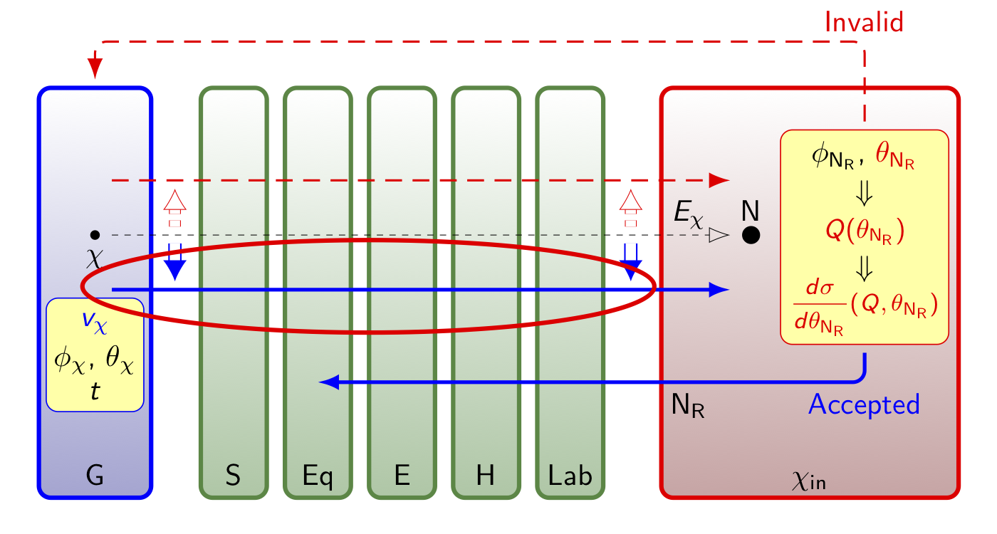
Figure 1: The workflow of our double–Monte Carlo simulation and data analysis procedure of 3-dimensional elastic WIMP–nucleus scattering. See the text for detailed descriptions.

In Ref. [13], we have

1. reviewed the MC generation of the 3-D velocity information (the magnitude, the direction, and the incoming/scattering time) of Galactic WIMPs,

2. summarized the definitions of and the transformations between all celestial coordinate systems.

In this section, we describe at first the overall workflow of our Monte Carlo scattering–by–scattering simulation of the 3-D elastic WIMP–nucleus scattering process. Then we review briefly the validation criterion of our Monte Carlo simulations by taking into account the cross section (nuclear form factor) suppression on each generated recoil energy.

2.1 Simulation workflow

In this subsection, we describe the overall workflow of our double–Monte Carlo simulation and data analysis procedure of 3-D elastic WIMP–nucleus scattering sketched in Fig. 1 in detail:

1. The 3-D velocity information of incident halo WIMPs (the magnitude and the direction as well as the incoming/scattering time) is MC generated according to a specified model of the Dark Matter halo in the Galactic coordinate system (the blue subframe) [11, 13].

2. The generated 3-D WIMP velocities will be transformed through the laboratory–independent (Ecliptic, Equatorial, and Earth) coordinate systems as well as the laboratory–dependent (horizontal and laboratory) coordinate systems (the green subframes) [11, 13] and at the end into the incoming–WIMP coordinate system (the red subframe) [13].

3. In the incoming–WIMP coordinate system, the 3-D elastic WIMP–nucleus scattering process will also be MC simulated by generating the orientation of the scattering plane $\phi_{\rm N_{R},\chi_{in}}$ and the “equivalent” recoil angle $\theta_{\rm N_{R},\chi_{in}}$ (defined in Fig. 2). They define the recoil direction of the scattered target nucleus and the latter, combined with the transformed WIMP incident velocity, will then be used for estimating the transferred recoil energy to the target nucleus, $Q(\theta_{\rm N_{R},\chi_{in}})$, and the differential WIMP–nucleus scattering cross section with respect to the recoil angle, $d\sigma/d\theta_{\rm N_{R},\chi_{in}}(Q,\theta_{\rm N_{R},\chi_{in}})$, in our event validation criterion (see Sec. 2.2).

4. The orientation of the scattering plane $\phi_{\rm N_{R},\chi_{in}}$ and the equivalent recoil angle $\theta_{\rm N_{R},\chi_{in}}$ of the accepted recoil events will be transformed (back) through all considered celestial coordinate systems (indicated by the lower solid blue arrow). All these 3-D recoil information of the scattered target nucleus accompanied with the corresponding recoil energy $Q$ as well as the 3-D velocity of the scattering WIMP in different coordinate systems (the upper solid blue arrow) will be recorded for further analyses.

5. For the invalid cases, in which the estimated recoil energies are out of the experimental measurable energy window or suppressed by the validation criterion, the generated 3-D information on the incident WIMP (the lower dashed red arrow) (and that on the scattered nucleus) will be discarded and the generation/validation process of one WIMP scattering event will be restarted from the Galactic coordinate system (the upper dashed red arrow).

2.2 Validation of 3-D elastic WIMP–nucleus scattering events

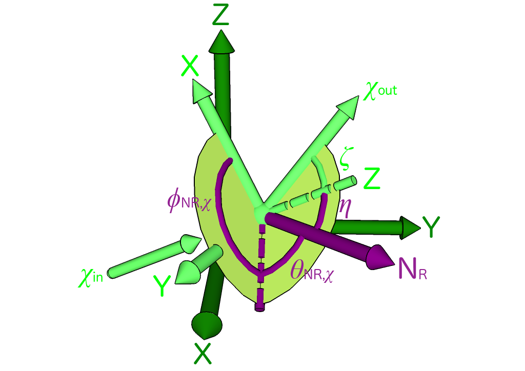
Figure 2: A 3-D elastic WIMP–nucleus scattering event in the (light–green) incoming–WIMP and the (dark–green) laboratory coordinate systems [11, 13]. $\zeta$ and $\eta$ are the scattering angle of the outgoing WIMP $\chi_{\rm out}$ and the recoil angle of the scattered target nucleus N_R measured in the incoming–WIMP coordinate system of this single scattering event, respectively. While the azimuthal angle of the recoil direction of the scattered nucleus N_R in this incoming–WIMP coordinate system, $\phi_{\rm N_{R},\chi_{in}}$, indicates the orientation of the scattering plane, the elevation of the recoil direction of N_R, $\theta_{\rm N_{R},\chi_{in}}$, is namely the complementary angle of the recoil angle $\eta$.

In Fig. 2, we sketch the process of one single 3-D elastic WIMP–nucleus scattering event: $\chi_{\rm in/out}$ indicate the incoming and the outgoing WIMPs, respectively. While $\zeta$ indicates the scattering angle of the outgoing WIMP $\chi_{\rm out}$ (measured from the ${\bf Z}_{\chi_{\rm in}}$–axis of the incoming–WIMP coordinate system, which is defined as the direction of the incident velocity of the incoming WIMP ${\bf v}_{\chi}$), $\eta$ is the recoil angle of the scattered target nucleus N_R. It can be found that the elevation of the recoil direction of the scattered nucleus, $\theta_{\rm N_{R},\chi_{in}}$, is namely the complementary angle of the recoil angle $\eta$. Thus, in our simulations, we can use

$$\theta_{\rm N_{R},\chi_{in}}\in[0,~{}\pi/2]$$ (1)

as the “equivalent” recoil angle. Since for one WIMP event transformed into the laboratory coordinate system with the velocity of ${\bf v}_{\chi}$, the kinetic energy can be given by

$$E_{\chi}=\frac{1}{2}m_{\chi}|{\bf v}_{\chi}|^{2}=\frac{1}{2}m_{\chi}v_{\chi,{\rm Lab}}^{2}~{}\!.$$ (2)

Then the recoil energy of the scattered target nucleus in the incoming–WIMP coordinate system can be estimated by the equivalent recoil angle $\theta_{\rm N_{R},\chi_{in}}$ as [13]

$$Q(\theta_{\rm N_{R},\chi_{in}})=\left[\left(\frac{2m_{\rm r,N}^{2}}{m_{\rm N}}\right)v_{\chi,{\rm Lab}}^{2}\right]\sin^{2}(\theta_{\rm N_{R},\chi_{in}})~{}\!,$$ (3)

where $m_{\rm r,N}\equiv m_{\chi}m_{\rm N}/(m_{\chi}+m_{\rm N})$ is the reduced mass of the WIMP mass $m_{\chi}$ and that of the target nucleus $m_{\rm N}$. And the differential cross section $d\sigma$ given by the absolute value of the momentum transfer from the incident WIMP to the recoiling target nucleus, $q=|{\bf q}|=\sqrt{2m_{\rm N}Q}$, can be obtained as [2, 13]

$$d\sigma=\frac{1}{v_{\chi,{\rm Lab}}^{2}}\left(\frac{\sigma_{0}}{4m_{\rm r,N}^{2}}\right)F^{2}(q)~{}\!dq^{2}=\sigma_{0}F^{2}(Q(\theta_{\rm N_{R},\chi_{in}}))\sin(2\theta_{\rm N_{R},\chi_{in}})~{}\!d\theta_{\rm N_{R},\chi_{in}}~{}\!.$$ (4)

Hence, the differential WIMP–nucleus scattering cross section with respect to the recoil angle $\theta_{\rm N_{R},\chi_{in}}$ can generally be given by [13]

$$\frac{d\sigma}{d\theta_{\rm N_{R},\chi_{in}}}=\bigg{[}\sigma_{0}^{\rm SI}F_{\rm SI}^{2}(Q(\theta_{\rm N_{R},\chi_{in}}))+\sigma_{0}^{\rm SD}F_{\rm SD}^{2}(Q(\theta_{\rm N_{R},\chi_{in}}))\bigg{]}\sin(2\theta_{\rm N_{R},\chi_{in}})~{}\!.$$ (5)

Here $\sigma_{0}^{\rm(SI,SD)}$ are the spin–independent (SI)/spin–dependent (SD) total cross sections ignoring the form factor suppression and $F_{\rm(SI,SD)}(Q)$ indicate the elastic nuclear form factors corresponding to the SI/SD WIMP interactions, respectively.

Finally, taking into account the proportionality of the WIMP flux to the incident velocity, the generating probability distribution of the recoil angle $\theta_{\rm N_{R},\chi_{in}}$, which is proportional to the scattering event rate of incident halo WIMPs with an incoming velocity $v_{\chi,{\rm Lab}}$ off target nuclei going into recoil angles of $\theta_{\rm N_{R},\chi_{in}}\pm d\theta_{\rm N_{R},\chi_{in}}/2$ with recoil energies of $Q\pm dQ/2$, can generally be given by [13]

$$f_{{\rm N_{R}},\chi_{\rm in},\theta}(\theta_{\rm N_{R},\chi_{in}})=\left(\frac{v_{\chi,{\rm Lab}}}{v_{\chi,{\rm cutoff}}}\right)\bigg{[}\sigma_{0}^{\rm SI}F_{\rm SI}^{2}(Q(\theta_{\rm N_{R},\chi_{in}}))+\sigma_{0}^{\rm SD}F_{\rm SD}^{2}(Q(\theta_{\rm N_{R},\chi_{in}}))\bigg{]}\sin(2\theta_{\rm N_{R},\chi_{in}})~{}\!,$$ (6)

where $v_{\chi,{\rm cutoff}}\simeq 800$ km/s is a cut–off velocity of incident halo WIMPs in the laboratory coordinate system.

3 3-D WIMP effective velocity distribution in the Equatorial frame

In Refs. [11] and [12], we demonstrated the angular distributions of the 3-D velocity (flux) and the kinetic energy of Galactic halo WIMPs impinging into (directional) direct DM detectors in different celestial coordinate systems, which show clearly the anisotropy and the directionality (the annual and the diurnal modulations). On the other hand, in Ref. [14], we have presented (the anisotropy and the directionality (the annual modulation) of) the angular distributions of the recoil direction (flux) as well as the accumulated and the average recoil energies of several frequently used target nuclei scattered by (simulated) incident Galactic WIMPs observed in different coordinate systems.

Then, in this and the next sections, we discuss correspondingly (the anisotropy and the directionality (the annual modulation) of) the 3-dimensional effective velocity distributions as well as the accumulated and the average kinetic energies of the (simulated) incident Galactic WIMPs scattering off target nuclei in the laboratory–independent Equatorial and Galactic coordinate systems, respectively.

Five (spin–sensitive) nuclei used frequently in (directional) direct detection experiments: ${}^{19}{\rm F}$, ${}^{40}{\rm Ar}$, ${}^{73}{\rm Ge}$, ${}^{129}{\rm Xe}$, and ${}^{183}{\rm W}$ have been considered as our targets. Then, while the SI (scalar) WIMP–nucleon cross section has been fixed as $\sigma_{\chi{\rm p}}^{\rm SI}=10^{-9}$ pb in our simulations presented in this paper, the effective SD (axial–vector) WIMP–proton/neutron couplings have been tuned as $a_{\rm p}=0.01$ and $a_{\rm n}=0.7a_{\rm p}=0.007$, respectively [13]. So that the contributions of the SI and the SD WIMP–nucleus cross sections (including the corresponding nuclear form factors) to the validation criterion (6) are approximately comparable for the considered ${}^{40}{\rm Ar}$, ${}^{73}{\rm Ge}$, and ${}^{129}{\rm Xe}$ target nuclei.

Moreover, in this paper we assume simply that the experimental threshold energies for all considered target nuclei are negligible, whereas the maximal experimental cut–off energy has been set as $Q_{\rm max}=100$ keV. 5,000 experiments with 500 accepted events on average (Poisson–distributed) in one observation period (365 days/year or 60 days/season) in one experiment for one laboratory/target nucleus have been simulated.

For readers’ reference, all simulation plots presented in this paper (and more) can be found “in animation” on our online (interactive) demonstration webpage [15].

3.1 Target dependence of the 3-D WIMP effective velocity distribution

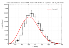
(a) ${}^{19}{\rm F}$

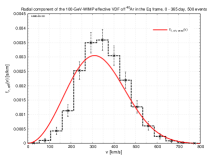
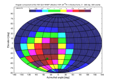
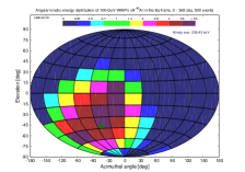
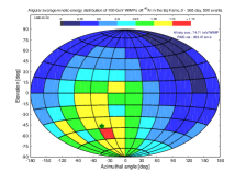
(b) ${}^{40}{\rm Ar}$

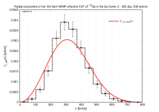
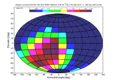
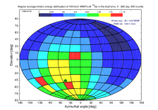
(c) ${}^{73}{\rm Ge}$

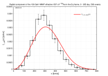
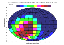
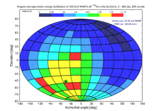
(d) ${}^{129}{\rm Xe}$

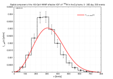
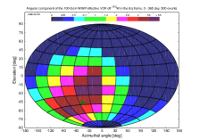
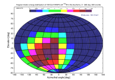
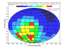
(e) ${}^{183}{\rm W}$

Figure 3: The radial (far–left) and the angular (center–left) components of the WIMP effective velocity distribution of the scattering WIMPs as well as the angular distributions of the corresponding accumulated (center–right) and average (far–right) WIMP kinetic energy in the Equatorial coordinate system. (Note that the angular distributions are in unit of the all–sky average values and the scale of the color bar used in the far–right column is different from that in the two central columns.) Five target nuclei: ${}^{19}{\rm F}$ (a), ${}^{40}{\rm Ar}$ (b), ${}^{73}{\rm Ge}$ (c), ${}^{129}{\rm Xe}$ (d), and ${}^{183}{\rm W}$ (e), have been presented. The mass of incident WIMPs has been set as $m_{\chi}=100$ GeV. 500 accepted WIMP scattering events on average in one entire year have been simulated and binned into 15 (radial) bins as well as 12 $\times$ 12 (angular) bins for the azimuthal angle and the elevation, respectively. The dark–green star indicates the theoretical main direction of incident WIMPs in the Equatorial coordinate system [16]: 42.00^∘S, 50.70^∘W. See the text for further details.

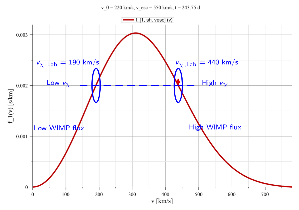
(a)

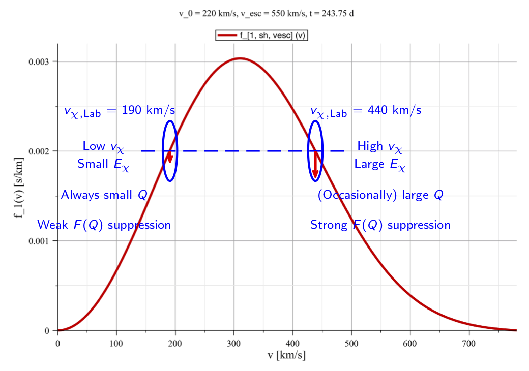
(b)

Figure 4: Two factors which cause the shift of the radial component (magnitude) of the 3-D WIMP effective velocity distribution: (a) the proportionality of the WIMP flux to the incident velocity (b) the cross section (nuclear form factor) suppression. See the text for the detailed arguments.

In Figs. 3, we show the radial (far–left) and the angular (center–left) components of the effective velocity distribution of the scattering WIMPs as well as the angular distributions of the corresponding accumulated (center–right) and average (far–right) WIMP kinetic energy in the Equatorial coordinate system (the angular distributions are in unit of the all–sky average values). Five target nuclei: ${}^{19}{\rm F}$, ${}^{40}{\rm Ar}$, ${}^{73}{\rm Ge}$, ${}^{129}{\rm Xe}$, and ${}^{183}{\rm W}$, have been presented here and the mass of incident WIMPs has been set as $m_{\chi}=100$ GeV. 500 accepted WIMP scattering events on average in one entire year have been simulated and binned into 15 (radial) bins as well as 12 $\times$ 12 (angular) bins for the azimuthal angle and the elevation, respectively. The dark–green star in each plot indicates the theoretical main direction of incident WIMPs in the Equatorial coordinate system: [16]: 42.00^∘S, 50.70^∘W.

As a reference, in the far–left column of Figs. 3, we draw the theoretically predicted shifted Maxwellian velocity distribution of halo WIMPs as the solid red curves [17]:

$$f_{1,{\rm sh},{\rm vesc}}(v_{\chi,{\rm Lab}})$$ (12)

$$= {\footnotesize\left\{\begin{array}[]{l l}\displaystyle N_{{\rm sh},{\rm vesc}}\left(\frac{v_{\chi,{\rm Lab}}}{v_{0}v_{\rm e}}\right)\Big{[}e^{-(v_{\chi,{\rm Lab}}-v_{\rm e})^{2}/v_{0}^{2}}-e^{-(v_{\chi,{\rm Lab}}+v_{\rm e})^{2}/v_{0}^{2}}\Big{]}~{}\!,&{\rm for}~{}v_{\chi,{\rm Lab}}\leq v_{\rm esc}-v_{\rm e}~{}\!,\\ {}&{}\\ \displaystyle N_{{\rm sh},{\rm vesc}}\left(\frac{v_{\chi,{\rm Lab}}}{v_{0}v_{\rm e}}\right)\Big{[}e^{-(v_{\chi,{\rm Lab}}-v_{\rm e})^{2}/v_{0}^{2}}-e^{-v_{\rm esc}^{2}/v_{0}^{2}}\Big{]}~{}\!,&{\rm for}~{}v_{\rm esc}-v_{\rm e}\leq v_{\chi,{\rm Lab}}\leq v_{\rm esc}+v_{\rm e}~{}\!,\\ {}&{}\\ 0~{}\!,&{\rm for}~{}v_{\chi,{\rm Lab}}\geq v_{\rm esc}+v_{\rm e}~{}\!,\end{array}\right.}$$

with the normalization constant

$$N_{{\rm sh},{\rm vesc}}=\left[\sqrt{\pi}~{}\!{\rm erf}{\displaystyle\left(\frac{v_{\rm esc}}{v_{0}}\right)}-\left(\frac{2v_{\rm esc}}{v_{0}}\right)e^{-v_{\rm esc}^{2}/v_{0}^{2}}\right]^{-1}~{}\!.$$ (13)

Here $v_{\rm e}$ is the time–dependent Earth’s velocity in the Galactic frame [18, 2]:

$$v_{\rm e}(t)=v_{0}\left[1.05+0.07\cos\left(\frac{2\pi(t-t_{\rm p})}{1~{}{\rm yr}}\right)\right]~{}\!,$$ (14)

with $t_{\rm p}\simeq$ June 2nd, the date on which the Earth’s orbital speed is maximal${}^{,~{}\!}$. Additionally, the thin vertical dashed black lines here indicate the 1$\sigma$ Poisson statistical uncertainties on the recorded event numbers.

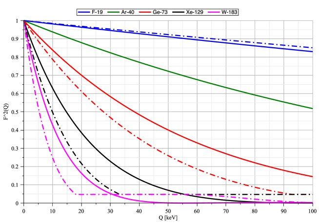
Figure 5: Nuclear form factors of the ${}^{19}{\rm F}$ (blue), the ${}^{40}{\rm Ar}$ (green), the ${}^{73}{\rm Ge}$ (red), the ${}^{129}{\rm Xe}$ (black), and the ${}^{183}{\rm W}$ (magenta) nuclei as functions of the recoil energy. The solid and dash–dotted curves indicate the form factors corresponding to the SI and SD cross sections adopted in our simulation package, respectively [13].

Firstly, from the radial distribution (magnitude) of the incoming velocity of incident WIMPs scattering off target nuclei shown in Figs. 3, the target–dependent discrepancy between the simulated histogram (the effective WIMP velocity distribution) and the theoretically predicted (shifted Maxwellian) velocity distribution can be seen obviously. The reason is follows.

Consider two subgroups of incident halo WIMPs with an equal velocity distribution value. For example, the moving velocities of two subgroup WIMPs are 190 km/s and 440 km/s, respectively. Then, as sketched in Fig. 4(a), since the WIMP flux is proportional to the incident velocity, the higher the velocity, the larger the flux and in turn the larger the scattering probability off target nuclei. However, as also sketched in Fig. 4(b), since the common velocity of the first subgroup of WIMPs is low and thus the common kinetic energy is small, they can only transfer small recoil energies to the scattered target nuclei. The reduction of the scattering probability of these WIMPs due to the (weak) cross section (nuclear form factor) suppression is then small or even negligible. In contrast, the common velocity of the second subgroup WIMPs is ($\sim$ 2.3 times) higher. So their common kinetic energy is ($\sim$ 5.4 times) larger and they could sometimes transfer (much) larger recoil energies to the scattered nuclei. However, the scattering probability of these large–recoil–energy events would be strongly reduced due to the sharply decreased cross section (nuclear form factor), especially with heavy target nuclei like ${}^{129}{\rm Xe}$ and ${}^{183}{\rm W}$ (see Fig. 5).

This indicates that, due to the cross section (nuclear form factor) suppression appearing in Eq. (6), the actual “effective” velocity distribution of incident halo WIMPs scattering off target nuclei should be (much) more strongly reduced from the theoretically predicted velocity distribution in the high velocity range than in the low velocity range. And the average velocity of the scattering WIMPs shifts to a lower velocity (than the theoretical prediction). In addition, as shown in Fig. 5, the heavier the target nucleus, the stronger the cross section (nuclear form factor) suppression (in the high energy range) and thus the larger the shift of the average velocity.

On the other hand, while the angular distribution patterns of the velocity direction (center–left) and the accumulated kinetic energy (center–right) of the scattering WIMPs look very similar to each other (but still slightly different) as well as to those of the entire incident WIMPs presented in Refs. [11, 12], the differences between the distribution patterns of the average WIMP kinetic energy (far–right) off different target nuclei and that of the entire incident WIMPs [12] seem somehow larger. Note here that, since the average velocity of WIMPs scattering off heavier target nuclei is lower and the all–sky average values of the accumulated and the average kinetic energies of the scattering WIMPs are in turn smaller, each distribution pattern shown in the same column of Figs. 3 is normalized by a different standard and demonstrates only the relative flux/kinetic energy of WIMPs with the simulated mass (e.g., $m_{\chi}=100$ GeV here) scattering off the considered target nucleus.

3.2 WIMP–mass dependence of the 3-D WIMP effective velocity distribution

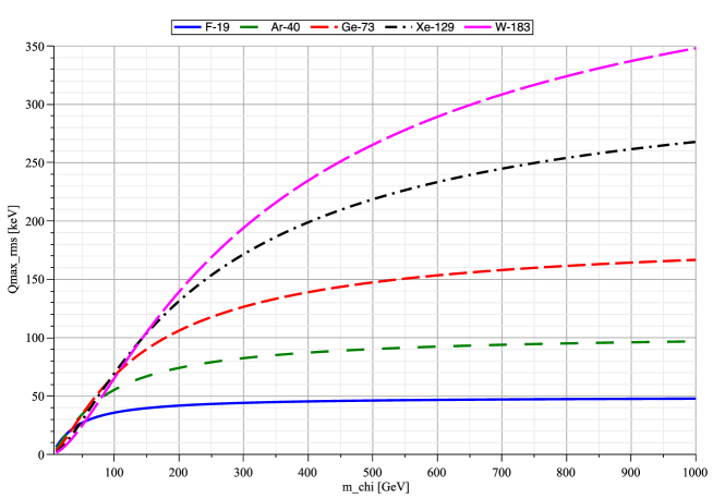
Figure 6: The WIMP–mass dependence of the maximum of the recoil energy, $Q_{\rm max,rms}$, given by Eq. (16). Five frequently used target nuclei: ${}^{19}{\rm F}$ (solid blue), ${}^{40}{\rm Ar}$ (rare–dashed green), ${}^{73}{\rm Ge}$ (dashed red), ${}^{129}{\rm Xe}$ (dash–dotted black), and ${}^{183}{\rm W}$ (long–dashed magenta) have been considered.

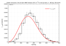
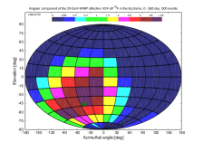
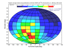
(a) ${}^{19}{\rm F}$

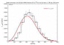
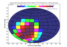
(b) ${}^{40}{\rm Ar}$

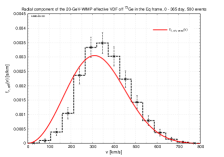
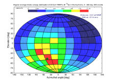
(c) ${}^{73}{\rm Ge}$

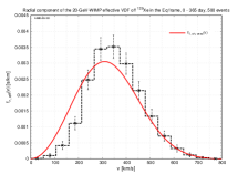
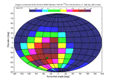
(d) ${}^{129}{\rm Xe}$

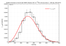
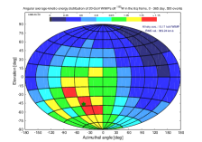
(e) ${}^{183}{\rm W}$

Figure 7: As in Figs. 3, except that the mass of incident WIMPs has been considered as light as $m_{\chi}=20$ GeV.

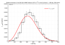
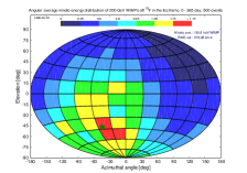
(a) ${}^{19}{\rm F}$

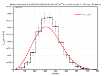
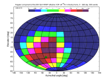
(b) ${}^{40}{\rm Ar}$

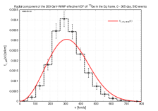
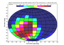
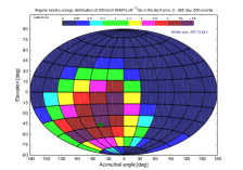
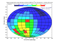
(c) ${}^{73}{\rm Ge}$

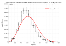
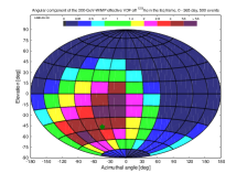
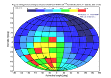
(d) ${}^{129}{\rm Xe}$

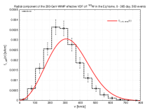
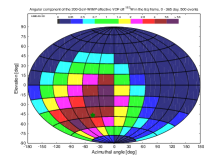
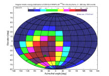
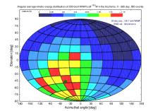
(e) ${}^{183}{\rm W}$

Figure 8: As in Figs. 7 and 3, except that the mass of incident WIMPs has been considered as heavy as $m_{\chi}=200$ GeV.

It is imaginable that, since the larger the mass of incident halo WIMPs, the larger their kinetic energy and the larger the maximal transferable recoil energy to the scattered target nuclei, the discrepancy between the effective velocity distribution of the scattering WIMPs and the theoretical prediction of the entire halo WIMPs caused by the cross section (nuclear form factor) suppression should be enlarged, once the WIMP mass becomes larger. More precisely, in Fig. 6, the WIMP–mass dependence of the maximum (prefactor) of the recoil energy $Q$ given by Eq. (3) with the root–mean–square (rms) velocity [13]

$$v_{\rm rms,Lab}^{2}=\left(\frac{3}{2}\right)v_{0}^{2}+v_{\rm e}^{2}\simeq(355~{}{\rm km/s})^{2}$$ (15)

as the common velocity of incident WIMPs:

$$Q_{\rm max,rms}=\left(\frac{2m_{\rm r,N}^{2}}{m_{\rm N}}\right)v_{\rm rms,Lab}^{2}~{}\!,$$ (16)

shows that the maximal recoil energy transferred by WIMPs increases basically with both of the increased mass of the target nucleus and that of incident WIMPs. Hence, in this subsection, we study the WIMP–mass dependence of the 3-D effective velocity distribution of the scattering WIMPs off different target nuclei in the Equatorial coordinated system in detail.

In Figs. 7 and 8, we show the radial (far–left) and the angular (center–left) components of the WIMP effective velocity distribution as well as the angular distributions of the accumulated (center–right) and average (far–right) WIMP kinetic energy (in unit of the all–sky average values) in the Equatorial coordinate system with a light WIMP mass of $m_{\chi}=20$ GeV and a heavy WIMP mass of 200 GeV, respectively.

It can be found that, once the mass of incident halo WIMPs is as light as ${\cal O}(20)$ GeV, the cross section (nuclear form factor) suppression is weak for all considered target nuclei and the factor of (the proportionality of the WIMP flux to) the incident velocity $v_{\chi,{\rm Lab}}$ appearing in Eq. (6) dominates. Hence, the magnitudes of the “20-GeV–WIMP” effective velocity distribution off all considered target nuclei shift towards the high velocity range and the differences between them are pretty small. Raising the simulated WIMP mass, the peaks of the WIMP effective velocity distribution and the average/rms velocities of the scattering WIMPs shift to lower velocities. The heavier the mass of the target nucleus, the larger the shift and the lower the average/root–mean–square velocities.

Meanwhile, the differences between the (characteristic) distribution patterns of the average WIMP kinetic energy (far–right) scattering off different target nuclei becomes also larger with the increased WIMP mass. For middle–mass and heavy target nuclei like ${}^{73}{\rm Ge}$ and ${}^{129}{\rm Xe}$, two extra hot–points close to the center and at the southwestern corner of the sky [12] would be more obvious than for light target nuclei like ${}^{19}{\rm F}$ and ${}^{40}{\rm Ar}$.

3.3 Annual modulation of the 3-D WIMP effective velocity distribution

Due to the orbital rotation of the Earth around the Sun, the relative velocity of incident halo WIMPs with respect to our laboratory/detector varies annually. Then the flux and the kinetic energy of incident WIMPs, the recoil energy of target nuclei scattered by incident WIMPs, as well as the WIMP effective velocity distribution should in turn vary annually. Hence, in this subsection, we discuss briefly the annual modulation of the 3-D effective velocity distribution of the scattering WIMPs in the Equatorial coordinated system.

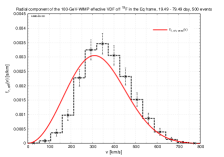
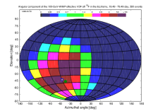
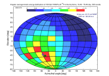
(a) 19.49 – 79.49 day

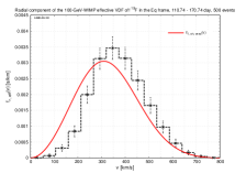
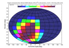
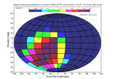
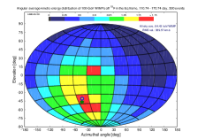
(b) 110.74 – 170.74 day

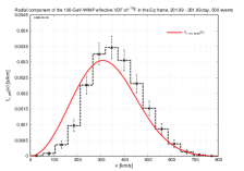
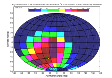
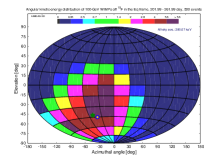
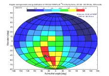
(c) 201.99 – 261.99 day

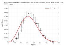
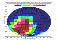
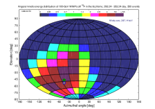
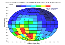
(d) 293.24 – 353.24 day

Figure 9: As in Figs. 3(a): ${}^{19}{\rm F}$ target nuclei scattered by 100-GeV WIMPs, except that 500 accepted events on average in each 60-day observation period of four advanced seasons [11, 13] have been considered. Besides the dark–green star indicating the theoretical main direction of the WIMP wind, the blue–yellow point in each plot indicates the opposite direction of the Earth’s movement in the Dark Matter halo on the central date of the observation period [11].

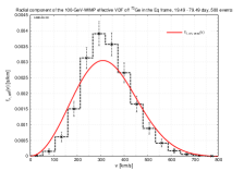
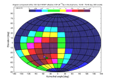
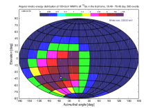
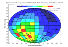
(a) 19.49 – 79.49 day

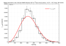
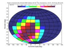
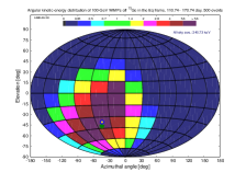
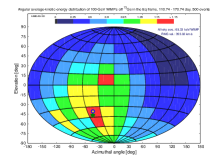
(b) 110.74 – 170.74 day

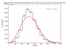
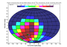
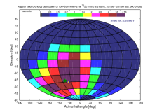
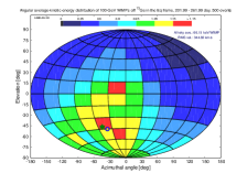
(c) 201.99 – 261.99 day

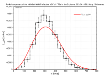
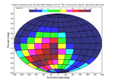
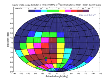
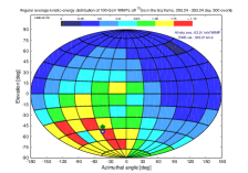
(d) 293.24 – 353.24 day

Figure 10: As in Figs. 9, except that a middle–mass nucleus ${}^{73}{\rm Ge}$ has been considered as our target.

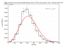
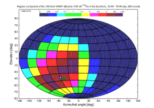
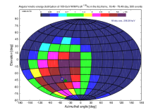
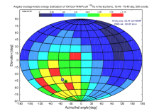
(a) 19.49 – 79.49 day

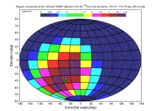
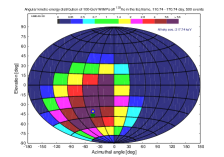
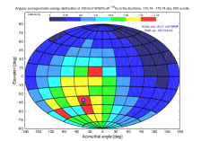
(b) 110.74 – 170.74 day

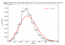
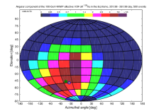
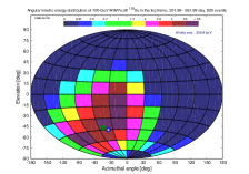
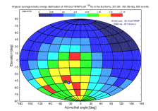
(c) 201.99 – 261.99 day

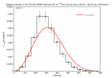
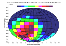
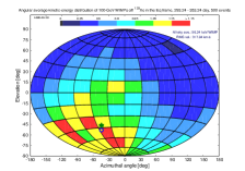
(d) 293.24 – 353.24 day

Figure 11: As in Figs. 9 and 10, except that a heavy nucleus ${}^{129}{\rm Xe}$ has been considered as our target.

In Figs. 9, 10, and 11, we show the radial (far–left) and the angular (center–left) components of the WIMP effective velocity distribution as well as the angular distributions of the accumulated (center–right) and the average (far–right) WIMP kinetic energy (in unit of the all–sky average values) in the Equatorial coordinate system with 500 accepted events on average in each 60-day observation period of four advanced seasons [11, 13]. 100-GeV WIMPs have been simulated to scatter off ${}^{19}{\rm F}$, ${}^{73}{\rm Ge}$, and ${}^{129}{\rm Xe}$ target nuclei, respectively. Besides the dark–green star indicating the theoretical main direction of the WIMP wind, the blue–yellow point in each plot indicates the opposite direction of the Earth’s movement in the Dark Matter halo on the central date of the observation period [11]. Additionally, for demonstrating the WIMP–mass dependence of the annual modulation of the 3-D WIMP effective velocity distribution in the Equatorial coordinate system, in Figs. 12, we raised the mass of incident WIMPs (scattering off ${}^{129}{\rm Xe}$) to $m_{\chi}=200$ GeV. Note that, the theoretically predicted shifted Maxwellian velocity distribution given in Eq. (12) with the time independent relation $v_{\rm e}=1.05~{}\!v_{0}$ has been used here for drawing the (fixed) solid red reference curves in the far–left column.

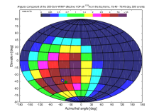
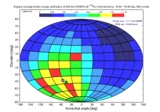
(a) 19.49 – 79.49 day

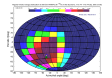
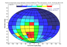
(b) 110.74 – 170.74 day

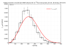
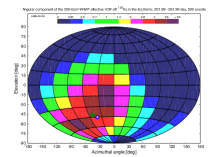
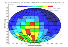
(c) 201.99 – 261.99 day

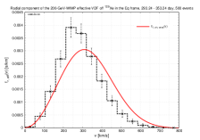
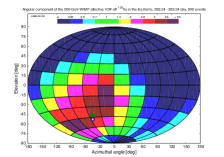
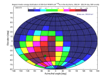
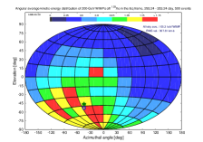
(d) 293.24 – 353.24 day

Figure 12: As in Figs. 11: ${}^{129}{\rm Xe}$ has been considered as the target nucleus, except that the mass of incident WIMPs has been raised to $m_{\chi}=200$ GeV.

It can be found that, firstly, for all considered target nuclei, the magnitude of the WIMP effective velocity distribution varies annually with maximal (minimal) average velocities in the advanced summer (winter). Meanwhile, the angular distributions of the velocity direction (flux) and the kinetic energy of the scattering WIMPs show the expected clockwise–rotated annual variations following the movement of the instantaneous theoretical main direction of incident WIMPs. From the (characteristic) distribution patterns of the average WIMP kinetic energy, one can even observe the target and WIMP–mass dependences.

4 3-D WIMP effective velocity distribution in the Galactic frame

The goal of directional direct Dark Matter detection experiments should not be limited to an identification of positive (annual/diurnal modulated) anisotropy of WIMP–nucleus scattering events and discriminating them from theoretically (approximately) isotropic/incoming–direction–known background/astrophysical events. A more important goal would be to understand the astrophysical and particle properties of Galactic WIMPs as well as the structure of Dark Matter halo. Hence, as a start, we discuss the 3-D effective velocity distribution of incident halo WIMPs in the Galactic coordinate system in this section.

4.1 Target dependence of the 3-D WIMP effective velocity distribution

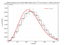
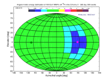
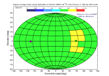
(a) ${}^{19}{\rm F}$

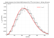
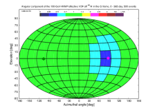
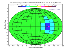
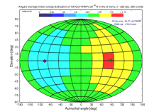
(b) ${}^{40}{\rm Ar}$

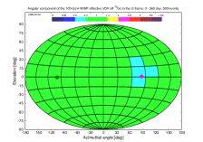
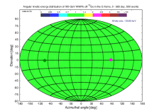
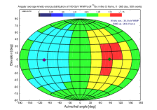
(c) ${}^{73}{\rm Ge}$

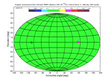
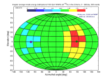
(d) ${}^{129}{\rm Xe}$

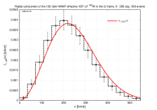
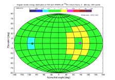
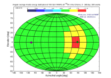
(e) ${}^{183}{\rm W}$

Figure 13: As in Figs. 3: 100-GeV WIMPs scatter off ${}^{19}{\rm F}$ (a), ${}^{40}{\rm Ar}$ (b), ${}^{73}{\rm Ge}$ (c), ${}^{129}{\rm Xe}$ (d), and ${}^{183}{\rm W}$ (e) nuclei, except that the 3-D information on the effective velocity distribution of the (simulated) incident halo WIMPs in the Galactic coordinate system has been presented. The solid red reference curves in the far–left column are the generating (simple Maxwellian) velocity distribution [13]. And the dark–green/purple star on the left–hand (western) sky of each plot indicates the theoretical main direction of incident WIMPs in the Galactic coordinate system [11, 13]: 0.60^∘S, 98.78^∘W, whereas the magenta/dark–green diamond on the right–hand (eastern) sky of each plot indicates additionally the moving direction of the Solar system in the Galactic coordinate system [11, 13]: 0.60^∘N, 81.22^∘E (see also Fig. 14(a)).

As in Sec. 3.1, we show the 3-D effective velocity distributions as well as the angular distributions of the corresponding accumulated and average kinetic energies of incident halo WIMPs scattering off five considered target nuclei: ${}^{19}{\rm F}$, ${}^{40}{\rm Ar}$, ${}^{73}{\rm Ge}$, ${}^{129}{\rm Xe}$, and ${}^{183}{\rm W}$, in the Galactic coordinate system in Figs. 13. The mass of incident WIMPs has been set as $m_{\chi}=100$ GeV and, as a reference, the solid red curves indicating the generating (simple Maxwellian) velocity distribution [13] have also been given in the far–left column. While the dark–green/purple star on the left–hand (western) sky of each plot indicates the theoretical main direction of incident WIMPs in the Galactic coordinate system [11, 13]: 0.60^∘S, 98.78^∘W, the magenta/dark–green diamond on the right–hand (eastern) sky of each plot indicates additionally the moving direction of the Solar system in the Galactic coordinate system [11, 13]: 0.60^∘N, 81.22^∘E (see Fig. 14(a) for a 3-dimensional sketch in the Galactic point of view).

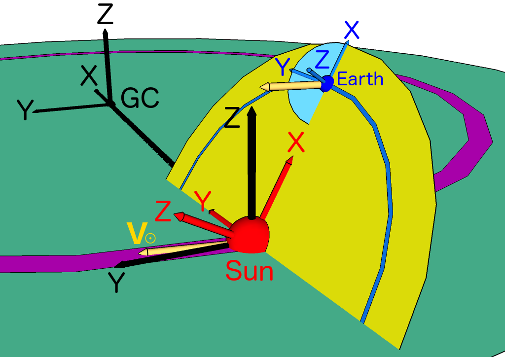
(a)

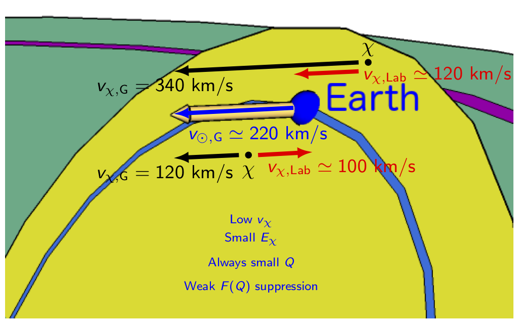
(b)

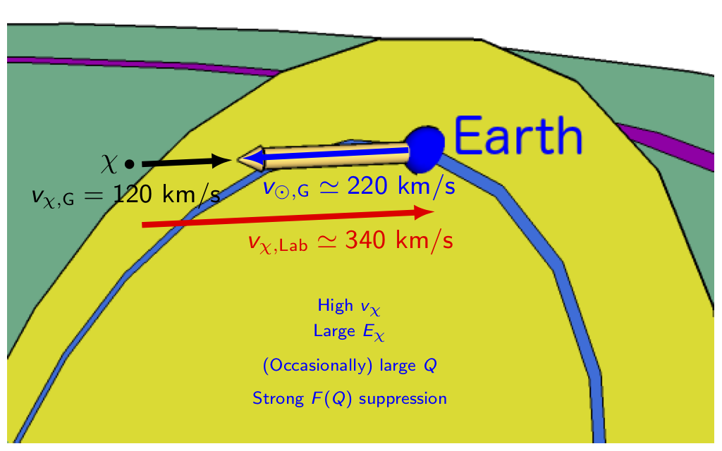
(c)

Figure 14: (a) The definitions of and the relative orientations between the (black) Galactic, the (red) Ecliptic, and the (blue) Equatorial coordinate systems (on the date of the vernal equinox) as well as the direction of the movement of the Solar system (the golden arrows) around the Galactic center (See Ref. [11] for details). The magenta circular band indicates an approximate path of the orbital motion of the Solar system in the Galaxy and the blue circular band indicates the Earth’s orbit around the Sun. (b)(c) The explanations of the anisotropy (forward–backward asymmetry) of the incident flux/kinetic energy of the 3-D WIMP effective velocity distribution due to the cross section (nuclear form factor) suppression. See the text for the detailed arguments.

Now, in the Galactic coordinate system, not only the target–dependent discrepancy of the magnitude of the 3-D WIMP effective velocity distribution from the generating velocity distribution, but also a target–dependent anisotropy of the moving direction (incident flux) as well as those of the angular distributions of the accumulate and the average kinetic energies can be observed clearly.

More precisely, firstly, the one–dimensional WIMP effective velocity distributions shown in the far–left column of Figs. 13 indicate that, as in the Equatorial coordinate system, the average Galactic velocity of incident 100-GeV halo WIMPs scattering off light (heavy) target nuclei like ${}^{19}{\rm F}$ and ${}^{40}{\rm Ar}$ (${}^{129}{\rm Xe}$ and ${}^{183}{\rm W}$) should be higher (lower) than that of the entire halo WIMPs.

Secondly and more importantly, the angular distribution patterns of the flux and the accumulated kinetic energy shown in two central columns of Figs. 13 indicate that WIMPs moving (approximately) in the same direction as the Galactic movement of our Solar system would have lower (higher) probabilities to scatter off light (heavy) target nuclei like ${}^{19}{\rm F}$ and ${}^{40}{\rm Ar}$ (${}^{129}{\rm Xe}$ and ${}^{183}{\rm W}$) than WIMPs moving (approximately) in the opposite direction of the movement of our Solar system. However, interestingly, the angular distributions of the average WIMP kinetic energy shown in the far–right column of Figs. 13 indicate that, for all considered target nuclei, the forwardly–moving (and scattering) WIMPs would have larger average kinetic energies (velocities) than the backwardly–moving WIMPs. Moreover, all distribution patterns in Figs. 13 show that such a “forward–backward asymmetry” of the 3-D WIMP effective velocity distribution in the Galactic coordinate system would itself be asymmetric: the increases (decreases) of the incident flux/kinetic energy of the forwardly–moving WIMPs are obviously (much) stronger than those of the backwardly–moving WIMPs.

The (asymmetric) forward–backward asymmetry of the 3-D WIMP Galactic effective velocity distribution is caused by the proportionality of the WIMP flux to the incident velocity as well as the cross section (nuclear form factor) suppression. Consider three cases. The first case: as sketched in Fig. 14(b), our Solar system moves in the Galactic coordinate system with a velocity of $v_{\rm\odot,G}\simeq 220$ km/s and a group of WIMPs moves (approximately) in the same direction with a small common velocity of $v_{\chi,{\rm G}}=120$ km/s. While, in the Galactic point of view, our detector would catch up WIMPs in this group from behind, in the laboratory/detector points of view, these WIMPs would hit our detector head–on with a relative velocity of $v_{\chi,{\rm Lab}}\simeq 100$ km/s. On the other hand, in the second case, a group of WIMPs moves also in the (approximately) same direction as our Solar system but with a larger common velocity of $v_{\chi,{\rm G}}=340$ km/s. In both of the Galactic and the laboratory/detector points of view, these WIMPs would catch up and hit our detector from behind with a relative velocity of $v_{\chi,{\rm Lab}}\simeq 120$ km/s. In both cases, as argued in Sec. 3.1, the relative velocities of incident WIMPs are low and their kinetic energies are small. Thus the WIMP fluxes are low, and the recoil energies transferred to the scattered target nuclei are always small, so that the cross section (nuclear form factor) suppression on the scattering probability of these WIMPs is weak or even negligible.

In contrast, consider the third case that a group of WIMPs moves in the opposite direction towards our Solar system with a common velocity as low as $v_{\chi,{\rm G}}=120$ km/s (see Fig. 14(c)). These WIMPs would hit our detector head–on with an ($\sim$ 3 times) higher incident velocity of $v_{\chi,{\rm Lab}}\simeq 340$ km/s and in turn a ($\sim$ 9 times) larger kinetic energy. So the WIMP fluxes are higher and the transferable recoil energies to the scattered target nuclei are (much) larger but practically almost always be suppressed, due to the (much) smaller cross section (nuclear form factor).

Furthermore, the “asymmetry” of the forward–backward asymmetry of the WIMP Galactic effective velocity distribution is also easy to understand. The relative velocities of the backwardly–moving WIMPs with respective to our laboratory/detector are at least $\sim$ 220 km/s. In contrast, the relatively velocity of the forwardly–moving WIMPs can be very low and the varying ranges of their incident fluxes, kinetic energies, and transferable recoil energies are much larger.

It would be worth to mention here that, although the radial component of the 100-GeV WIMP effective velocity distribution off ${}^{73}{\rm Ge}$ nuclei shown in Figs. 13(c) seems to match the generating velocity distribution perfectly, the anisotropy of the angular distribution of the average kinetic energy could still be observed clearly.

4.2 WIMP–mass dependence of the 3-D WIMP effective velocity distribution

As in Sec. 3.2, in this subsection, we consider the WIMP–mass dependence of the 3-D WIMP effective velocity distribution in the Galactic coordinated system.

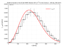
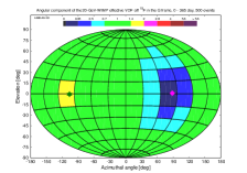
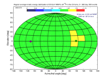
(a) ${}^{19}{\rm F}$

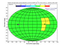
(b) ${}^{40}{\rm Ar}$

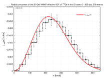
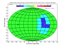
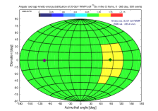
(c) ${}^{73}{\rm Ge}$

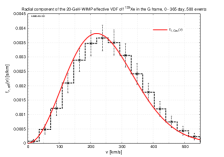
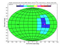
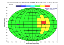
(d) ${}^{129}{\rm Xe}$

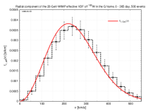
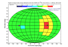
(e) ${}^{183}{\rm W}$

Figure 15: As in Figs. 13, except that the mass of incident WIMPs has been considered as light as $m_{\chi}=20$ GeV.

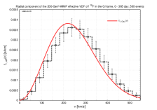
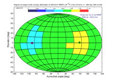
(a) ${}^{19}{\rm F}$

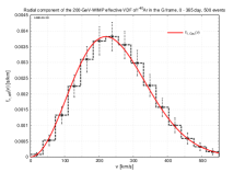
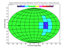
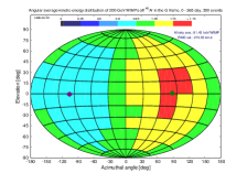
(b) ${}^{40}{\rm Ar}$

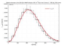
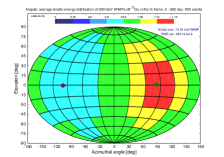
(c) ${}^{73}{\rm Ge}$

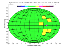
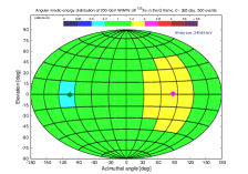
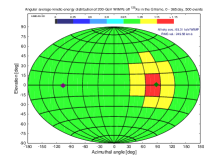
(d) ${}^{129}{\rm Xe}$

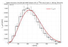
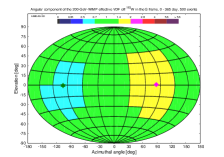
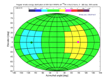
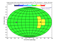
(e) ${}^{183}{\rm W}$

Figure 16: As in Figs. 15, and 13, except that the mass of incident WIMPs has been considered as heavy as $m_{\chi}=200$ GeV.

In Figs. 15 and 16, we show the 3-D effective velocity distributions as well as the angular distributions of the corresponding accumulated and average kinetic energies of incident halo WIMPs scattering off five considered target nuclei in the Galactic coordinate system. A light WIMP mass of $m_{\chi}=20$ GeV and a heavy one of 200 GeV have been simulated.

It can be seen clearly that, firstly, for the case of the light WIMP mass of $m_{\chi}=20$ GeV, the proportionality of the incident flux to the WIMP velocity dominates and thus the forwardly–moving WIMPs would have lower scattering probabilities off all considered target nuclei, but larger average kinetic energies, compared to the all–sky average values. Secondly, as already discussed in Sec. 3.2, once the mass of incident WIMPs becomes larger, the differences between the one–dimensional WIMP effective velocity distribution as well as the angular distribution patterns of the velocity direction/kinetic energy of the scattering WIMPs off different target nuclei would indeed be more and more obvious. It would be worth to note here that, not like the distribution patterns in the Equatorial coordinate system demonstrated in Sec. 3, even for the case of the light WIMP mass of $m_{\chi}=20$ GeV, the target dependence of the angular distribution patterns of the velocity direction/kinetic energy in the Galactic coordinate system could be observed clearly.

4.3 Annual modulation of the 3-D WIMP effective velocity distribution

In Sec. 3.3, we have demonstrated the (target and WIMP–mass dependent) annual modulation of the 3-D WIMP effective velocity distribution off different target nuclei in the Equatorial coordinate system. Considering the more clear target and WIMP–mass dependences and the interesting forward–backward asymmetry of the 3-D WIMP effective velocity distribution in the Galactic coordinate system, it would then be reasonable to study and demonstrate here its annual modulation.

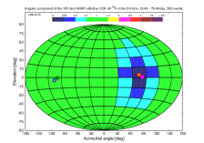
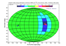
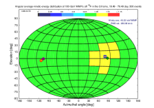
(a) 19.49 – 79.49 day

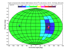
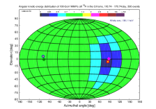
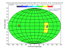
(b) 110.74 – 170.74 day

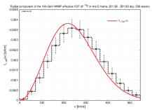
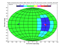
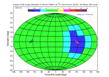
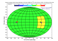
(c) 201.99 – 261.99 day

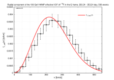
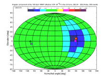
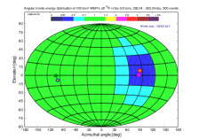
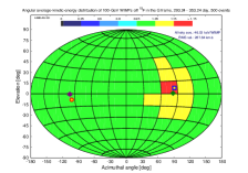
(d) 293.24 – 353.24 day

Figure 17: As in Figs. 13(a): ${}^{19}{\rm F}$ target nuclei scattered by 100-GeV WIMPs, except that 500 accepted events on average in each 60-day observation period of four advanced seasons [11, 13] have been considered. Besides the dark–green/purple star indicating the theoretical main direction of the WIMP wind and the magenta/dark–green diamond indicating the direction of the Solar Galactic movement, (the blue/red–yellow point and) the red/blue–yellow square in each plot indicate the (opposite) direction of the Earth’s movement in the Dark Matter halo on the central date of the observation period [11].

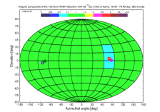
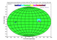
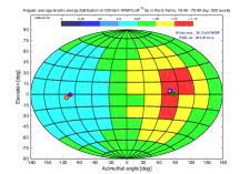
(a) 19.49 – 79.49 day

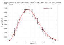
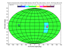
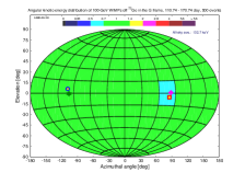
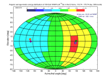
(b) 110.74 – 170.74 day

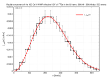
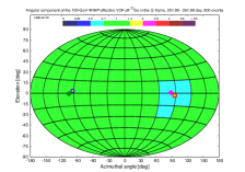
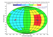
(c) 201.99 – 261.99 day

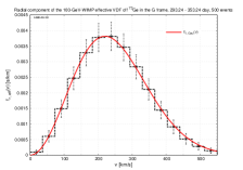
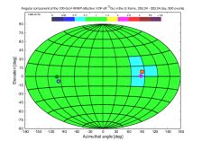
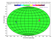
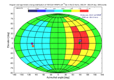
(d) 293.24 – 353.24 day

Figure 18: As in Figs. 17, except that a middle–mass nucleus ${}^{73}{\rm Ge}$ has been considered as our target.

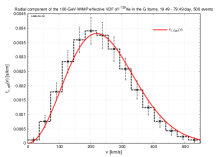
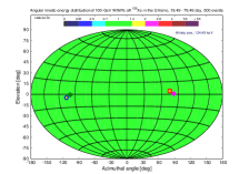
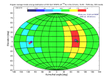
(a) 19.49 – 79.49 day

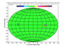
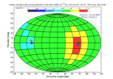
(b) 110.74 – 170.74 day

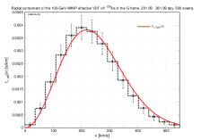
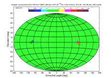
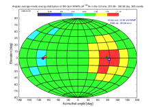
(c) 201.99 – 261.99 day

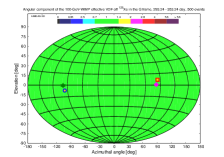
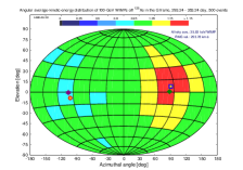
(d) 293.24 – 353.24 day

Figure 19: As in Figs. 17 and 18, except that a heavy nucleus ${}^{129}{\rm Xe}$ has been considered as our target.

In Figs. 17, 18, and 19, we show the 3-D effective velocity distributions as well as the angular distributions of the accumulated and the average kinetic energies of the scattering WIMPs in the Galactic coordinate system with 500 accepted events on average in each 60-day observation period of four advanced seasons. 100-GeV WIMPs have been simulated to scatter off ${}^{19}{\rm F}$, ${}^{73}{\rm Ge}$, and ${}^{129}{\rm Xe}$ target nuclei, respectively. Besides the dark–green/purple star indicating the theoretical main direction of the WIMP wind and the magenta/dark–green diamond indicating the direction of the Solar Galactic movement, (the blue/red–yellow point and) the red/blue–yellow square in each plot indicate the (opposite) direction of the Earth’s movement in the Dark Matter halo on the central date of the observation period [11].

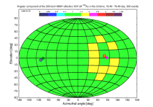
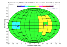
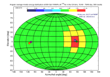
(a) 19.49 – 79.49 day

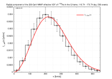
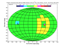
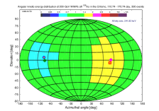
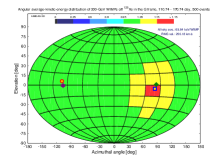
(b) 110.74 – 170.74 day

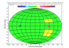
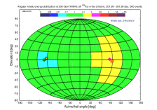
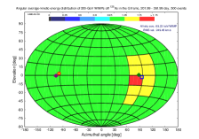
(c) 201.99 – 261.99 day

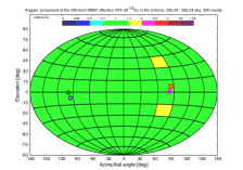
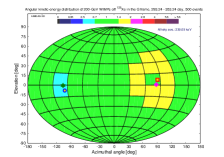
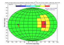
(d) 293.24 – 353.24 day

Figure 20: As in Figs. 19: ${}^{129}{\rm Xe}$ has been considered as the target nucleus, except that the mass of incident WIMPs has been raised to $m_{\chi}=200$ GeV.

Firstly, in contrast to the variations of the one–dimensional (incident) velocity distribution of the scattering WIMPs in the Equatorial (laboratory) coordinate system shown in the far–left columns of Figs. 9 to 12, the average Galactic velocity of light WIMPs scattering off light target nuclei like ${}^{19}{\rm F}$ and ${}^{40}{\rm Ar}$ would be minimal (maximal) in the advanced summer (winter). However, once the WIMP mass is as large as $m_{\chi}\>\raisebox{-3.01385pt}{$\stackrel{{\scriptstyle\textstyle>}}{{\sim}}$}\>~{}\!{\cal O}(200)$ GeV, the average WIMP Galactic velocity scattering off heavy target nuclei like ${}^{129}{\rm Xe}$ and ${}^{183}{\rm W}$ would reversely become maximal (minimal) in summer (winter). In Table 1, we give the summary of the (advanced) season, in which the average Galactic velocity of the scattering WIMPs off the considered target nucleus would be maximal.

Season of the maximal average Galactic velocity of the scattering WIMPs
Target nucleus	WIMP mass
	20 GeV	50 GeV	100 GeV	200 GeV	500 GeV
${}^{19}{\rm F}$
${}^{40}{\rm Ar}$	Winter
${}^{73}{\rm Ge}$					${}^{~{}}$Winter†
${}^{129}{\rm Xe}$			${}^{~{}}$Winter†	Summer
${}^{183}{\rm W}$

Table 1: The summary of the (advanced) season, in which the average Galactic velocity of the scattering WIMPs off the considered target nucleus would be maximal.
^†: Determined by the one–dimensional WIMP effective velocity distribution shown in the far–left columns of Figs. 17 to 20.

Secondly and very importantly, it could also be found that the angular distribution patterns of the velocity direction/kinetic energy of the scattering WIMPs on the eastern sky indeed rotate (approximately) counterclockwise following (the red/blue–yellow square indicating) the instantaneous Earth’s movement in the Dark Matter halo, while the distribution patterns on the western sky rotate synchronously (and approximately) clockwise following (the blue/red–yellow point indicating) the instantaneous theoretical main direction of incident WIMPs. All (light and heavy) considered target nuclei would demonstrate this subtle annual variation of the forward–backward asymmetry.

Finally, for the sake of completeness, in Figs. 20 we raise the mass of incident WIMPs to $m_{\chi}=200$ GeV for demonstrating the WIMP–mass dependence of the annual modulation of the 3-D WIMP effective velocity distribution in the Galactic coordinate system. As expected, the annual modulations of the anisotropy of the angular distribution patterns of the velocity direction/kinetic energy of the scattering WIMPs becomes more obvious.

5 Summary

In this paper, as the counterpart of our study on the angular distributions of the recoil direction (flux) and the recoil energy of the (Monte Carlo simulated) WIMP–scattered target nuclei [14], we investigated the corresponding 3-dimensional effective velocity distribution of WIMPs scattering off target nuclei in different celestial coordinate systems.

Besides the proportionality of the incident flux to the WIMP velocity, we took into account the cross section (nuclear form factor) suppression on the transferred recoil energy in our double–Monte Carlo scattering–by–scattering simulation of the 3-dimensional elastic WIMP–nucleus scattering process and demonstrated the 3-D WIMP effective velocity distributions off several frequently used target nuclei in the Equatorial and the Galactic coordinate systems, which, instead of the theoretical predictions of the entire group of Galactic Dark Matter particles, describe the actual velocity distributions of WIMPs scattering off (specified) target nuclei in an underground detector.

Our simulations showed that, firstly, in both of the Equatorial and the Galactic coordinate systems, there are clear discrepancies between the radial components (magnitudes) of the 3-D WIMP effective velocity distributions and the theoretically predicted and generating one–dimensional velocity distributions of the entire group of incident WIMPs. Such discrepancies depend on the target nucleus as well as on the mass of incident halo WIMPs: once the WIMP mass is as small as only $\cal O$(20) GeV, the proportionality of the WIMP flux to the incident velocity dominates and the average velocity/kinetic energy of the scattering WIMPs off all considered target nuclei would be larger than those of the entire halo WIMPs; with the increased WIMP mass, the average velocity of the scattering WIMPs shifts towards to lower velocities; the heavier the mass of the target nucleus, the larger the shift.

Secondly and more importantly, the angular components (directions/fluxes) of the 3-D WIMP effective velocity distributions as well as the angular distributions of the accumulated kinetic energy of the scattering WIMPs in not only the Equatorial/laboratory but also the Galactic coordinate systems show clear target and WIMP–mass dependent anisotropies, which indicate the forward–backward asymmetry of the scattering rate of incident halo WIMPs: WIMPs moving in the same direction as the Galactic movement of the Solar system or, more precisely, that of our laboratory/detector would have a higher (lower) probability to scatter off heavy (light) target nuclei than WIMPs moving in the opposite direction of the moving direction of the Solar system and our laboratory/detector. However, interestingly, for all considered target nuclei, the forwardly–moving (and scattering) WIMPs would have larger average velocities/kinetic energies than the backwardly–moving WIMPs.

Moreover, the magnitudes of the 3-D WIMP effective velocity distributions in not only the Equatorial/laboratory but also the Galactic coordinate systems vary annually with the target and WIMP–mass dependences. Interestingly, while the average velocity of the scattering WIMPs in the Equatorial coordinate system would be maximal (minimal) in the advanced summer (winter), the average WIMP velocity in the Galactic coordinate system would reversely be minimal (maximal) in summer (winter), except of heavy ($m_{\chi}\>\raisebox{-3.01385pt}{$\stackrel{{\scriptstyle\textstyle>}}{{\sim}}$}\>~{}\!{\cal O}(200)$ GeV) WIMPs scattering off heavy target nuclei like ${}^{129}{\rm Xe}$ and ${}^{183}{\rm W}$.

In our simulations presented in this paper, 500 accepted WIMP–scattering events on average in one observation period (365 days/year or 60 days/season) in one experiment for one laboratory/target nucleus have been simulated. Regarding the observation periods considered in our simulations presented in this paper, we used several approximations about the Earth’s orbital motion in the Solar system. First, the Earth’s orbit around the Sun is perfectly circular on the Ecliptic plane and the orbital speed is thus a constant. Second, the date of the vernal equinox is exactly fixed at the end of the May 20th (the 79th day) of a 365-day year and the few extra hours in an actual Solar year have been neglected. Nevertheless, considering the very low WIMP scattering event rate and thus maximal a few (tens) of total (combined) WIMP events observed in at least a few tens (or even hundreds) of days (an optimistic overall event rate of $\>\raisebox{-3.01385pt}{$\stackrel{{\scriptstyle\textstyle<}}{{\sim}}$}\>~{}\!{\cal O}(1)$ event/day) for the first–phase analyses, these approximations should be acceptable.

In summary, we finally achieved the full Monte Carlo scattering–by–scattering simulation of the 3-dimensional elastic WIMP–nucleus scattering process and can provide experimentally measurable (pseudo)data: the 3-dimensional recoil direction and the recoil energy of the WIMP–scattered target nuclei as well as the 3-D velocity/kinetic energy of the scattering WIMPs. Several important (but unexpected) characteristics have been observed. Hopefully, this (and more works fulfilled in the future) could help our colleagues to develop analysis methods for understanding the astrophysical and particle properties of Galactic WIMPs as well as the structure of Dark Matter halo by using directional direct detection data.

Acknowledgments

The author would like to thank the pleasant atmosphere of the W101 Ward and the Cancer Center of the Kaohsiung Veterans General Hospital, where part of this work was completed. This work was strongly encouraged by the “Researchers working on e.g. exploring the Universe or landing on the Moon should not stay here but go abroad.” speech.

References

- [1]
- [2] G. Jungman, M. Kamionkowski and K. Griest, “Supersymmetric Dark Matter”, Phys. Rep. 267, 195–373 (1996), arXiv:hep-ph/9506380.
- [3] R. J. Gaitskell, “Direct Detection of Dark Matter”, Ann. Rev. Nucl. Part. Sci. 54, 315–359 (2004).
- [4] L. Baudis, “Direct Dark Matter Detection: the Next Decade”, Issue on “The Next Decade in Dark Matter and Dark Energy”, Phys. Dark Univ. 1, 94–108 (2012), arXiv:1211.7222 [astro-ph.IM].
- [5] L. Baudis and S. Profumo, contribution to “The Review of Particle Physics 2020”, Prog. Theor. Exp. Phys. 2020, 083C01 (2020), 27. Dark Matter.
- [6] S. Ahlen et al., “The Case for a Directional Dark Matter Detector and the Status of Current Experimental Efforts”, Int. J. Mod. Phys. A25, 1–51 (2010), arXiv:0911.0323 [astro-ph.CO].
- [7] F. Mayet et al., “A Review of the Discovery Reach of Directional Dark Matter Detection”, Phys. Rept. 627, 1–49 (2016), arXiv:1602.03781 [astro-ph.CO].
- [8] J. B. R. Battat et al., “Readout Technologies for Directional WIMP Dark Matter Detection”, Phys. Rept. 662, 1–46 (2016), arXiv:1610.02396 [physics.ins-det].
- [9] CYGNUS Collab., S. E. Vahsen et al., “CYGNUS: Feasibility of a Nuclear Recoil Observatory with Directional Sensitivity to Dark Matter and Neutrinos”, arXiv:2008.12587 [physics.ins-det] (2020).
- [10] S. E. Vahsen, C. A. J. O’Hare and D. Loomba, “Directional Recoil Detection”, Ann. Rev. Nucl. Part. Sci. xx, 1–45 (2021), arXiv:2102.04596 [physics.ins-det].
- [11] C.-L. Shan, “Simulations of the 3-Dimensional Velocity Distribution of Halo Weakly Interacting Massive Particles for Directional Dark Matter Detection Experiments”, arXiv:1905.11279 [astro-ph.HE] (2019), in publication.
- [12] C.-L. Shan, “Simulations of the Angular Kinetic–Energy Distribution of Halo Weakly Interacting Massive Particles for Directional Dark Matter Detection Experiments”, in publication.
- [13] C.-L. Shan, “Monte Carlo Scattering–by–Scattering Simulation of 3-Dimensional Elastic WIMP–Nucleus Scattering Events”, arXiv:2103.xxxxx [hep-ph] (2021).
- [14] C.-L. Shan, “Simulations of the Angular Recoil–Energy Distribution of WIMP–Scattered Target Nuclei for Directional Dark Matter Detection Experiments”, arXiv:2103.xxxxx [hep-ph] (2021).
- [15] C.-L. Shan, online interactive demonstrations of 3-dimensional WIMP–nucleus elastic scattering for (directional) direct Dark Matter detection experiments and phenomenology, http://www.tir.tw/phys/hep/dm/amidas-2d/ (2021).
- [16] A. Bandyopadhyay and D. Majumdar, “On Diurnal and Annual Variations of Directional Detection Rates of Dark Matter”, Astrophys. J. 746, 107 (2012), arXiv:1006.3231 [hep-ph].
- [17] J. D. Lewin and P. F. Smith, “Review of Mathematics, Numerical Factors, and Corrections for Dark Matter Experiments Based on Elastic Nuclear Recoil”, Astropart. Phys. 6, 87–112 (1996).
- [18] K. Freese, J. Frieman and A. Gould, “Signal Modulation in Cold–Dark–Matter Detection”, Phys. Rev. D37, 3388–3405 (1988).