Revealing three-dimensional quantum criticality by Sr-substitution in Han Purple

Abstract

Classical and quantum phase transitions (QPTs), with their accompanying concepts of criticality and universality, are a cornerstone of statistical thermodynamics. An excellent example of a controlled QPT is the field-induced ordering of a gapped quantum magnet. Although numerous “quasi-one-dimensional” coupled spin-chain and -ladder materials are known whose ordering transition is three-dimensional (3D), quasi-2D systems are special for multiple reasons. Motivated by the ancient pigment Han Purple (BaCuSi₂O₆), a quasi-2D material displaying anomalous critical properties, we present a complete analysis of Ba_0.9Sr_0.1CuSi₂O₆. We measure the zero-field magnetic excitations by neutron spectroscopy and deduce the spin Hamiltonian. We probe the field-induced transition by combining magnetization, specific-heat, torque, and magnetocalorimetric measurements with nuclear magnetic resonance studies near the QPT. By a Bayesian statistical analysis and large-scale Quantum Monte Carlo simulations, we demonstrate unambiguously that observable 3D quantum critical scaling is restored by the structural simplification arising from light Sr-substitution in Han Purple.

I Introduction

At a continuous classical or quantum phase transition (QPT), characteristic energy scales vanish, characteristic (“correlation”) lengths diverge and hence the properties of the system are dictated only by global and scale-invariant quantities Zinn-Justin2002. The critical properties at the transition then depend only on factors such as the dimensionality of the system, the symmetry group of the order parameter, and in some cases on topological criteria. These fundamental factors are not all independent, but are all discrete, and as a result phase transitions can be categorized by their “universality class.”

An instructive example of the effects of dimensionality is found for systems where the U(1) symmetry of the order parameter is broken Pitaevskii2016. For free bosons, the symmetry-broken phase is the Bose-Einstein condensate (BEC) Bose1924; Einstein1924 and, while most familiar in three dimensions (3D), this transition can in fact be found in systems whose effective dimension is any real number $d>2$. However, strictly in 2D the physics is quite different, dependent on the binding of point vortices, and the system displays the Berezinskii-Kosterlitz-Thouless (BKT) transition Berezinskii1971; Kosterlitz1973. In real materials, the issue of system dimensionality is complicated by the fact that the coupling of different subsystems (such as clusters, chains, or planes) may occur on different low energy scales that are only revealed as the temperature is lowered. Strict 1D or 2D behavior is avoided because, as the critical point is approached on the low-dimensional subsystem, the growing correlation length causes the subsystems to become entangled and the critical properties are expected to be those associated with a 3D universality class Giamarchi2003; Sachdev2011.

Dimerized quantum spin systems, composed of strongly coupled pairs of spin-1/2 ions, constitute a particularly valuable class of materials for the study of quantum criticality. For sufficiently strong dimerization, the zero-field ground state of local singlets is always gapped, with the excitations taking the form of propagating local triplet quasiparticles (“triplons”). In an applied magnetic field, this system undergoes a QPT at which the gap is closed and the new ground state has field-induced transverse magnetic order, which can be described as a triplon condensate Nikuni2000; Rice2002; Giamarchi2008; Zapf2014. This is a 3D QPT from a quantum disordered phase with U(1) (or XY) symmetry to a BEC phase, whose emerging long-range magnetic order breaks the U(1) symmetry. This QPT has been studied extensively in materials where the inter-dimer coupling is similar in all three spatial dimensions Rueegg2003; Giamarchi2008. In gapped quasi-1D materials (dimerized chains, Haldane chains, two-leg ladders), fields exceeding the gap reveal the physics of the Tomonaga-Luttinger liquid at higher temperatures, but 3D scaling behavior is restored in the quantum critical regime around the QPT Klanjsek2008; Thielemann2008; Schmidiger2012; Mukhopadhyay2012; Blinder2017; Tsirlin2019. However, 2D systems with continuous symmetry are special because of the Mermin-Wagner theorem Mermin1966, and extra-special because of BKT physics Berezinskii1971; Kosterlitz1973, which has recently been argued to give rise to behavior at the dimensional crossover that is radically different from the 0D and 1D cases Furuya2016. Thus the question arises as to whether the “conventional” emergence of 3D physics can really be expected at the field-induced QPT in a quasi-2D material.

Unfortunately the list of candidate quasi-2D spin-dimer compounds suitable for answering this question is rather short. One well-studied material is SrCu₂(BO₃)₂ Kageyama1999, which displays a wealth of fascinating physics as a consequence of its ideally frustrated Shastry-Sutherland geometry Sutherland1981. While this includes magnetization plateaus Momoi2000; Kodama2002; Takigawa2013 and topological phases Romhanyi2015 in an applied field, first-order QPTs to plaquette Corboz2013; Corboz2014 and antiferromagnetic (AF) phases under applied pressure Waki2007; Takigawa2010; Haravifard2012; Zayed2017; Sakurai2018, proliferating bound-state excitations, and anomalous thermodynamics Wietek2019, it does not include the type of physics we discuss. The compound (C₄H₁₂N₂)Cu₂Cl₆ was also an early candidate due to its well-separated planes of Cl-coordinated Cu dimers, but was found to possess complicated and frustrated 3D coupling Stone2001 and to display an unexpected breakdown of triplon excitations due to strong mutual scattering Stone2006. The chromate compounds Ba₃Cr₂O₈ Nakajima2006; Kofu2009; Aczel2009a and Sr₃Cr₂O₈ Aczel2009b; Nomura2020 form $S=1/2$ dimer units in a triangular geometry and show 3D scaling at the field-induced QPT, but structural distortion and magnetic frustration effects leave their dominant dimensionality (2D or 1D) unconfirmed.

A further prominent material, which does actually realize 2D square lattices of dimers and a field-induced triplon condensation at $\mu_{0}H_{c1}\simeq 23.5$ T, is the ancient pigment Han Purple (BaCuSi₂O₆) Jaime2004; Sebastian2005. In this compound the stacked dimer bilayers have a body-centered offset, leading to the expectation of an exact frustration of AF coupling between successive bilayers, and further to the interpretation of thermodynamic measurements showing apparent 2D scaling close to the QPT Sebastian2006 as a frustration-induced “dimensional reduction” quite different from 3D critical properties. However, it was shown subsequently that the weakly orthorhombic structure of this material below 90 K Samulon2006; Sparta2006; Stern2014 contains three types of structurally Sheptyakov2012 and magnetically Horvatic2005; Rueegg2007; Kraemer2007 inequivalent bilayers, and later that the inter-bilayer coupling is not in fact frustrated Mazurenko2014; Allenspach2020. These properties lead ultimately to a regime of anomalous effective scaling in the experimentally accessible parameter space Allenspach2020, with the 3D critical behavior remaining unobservable.

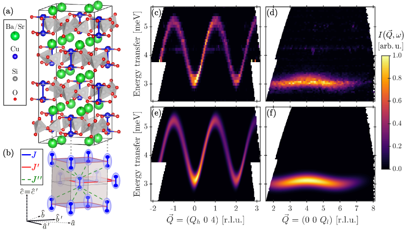
Figure 1: Structure and inelastic neutron spectrum of Ba_0.9Sr_0.1CuSi₂O₆. (a) Tetragonal crystallographic structure of Ba_0.9Sr_0.1CuSi₂O₆ Puphal2016. (b) Representation of the minimal magnetic unit cell, indicating the relevant Heisenberg interaction parameters between dimers on the two bilayers, which are structurally equivalent with body-centered geometry. $({\hat{a}},{\hat{b}},{\hat{c}})$ and $({\hat{a}}^{\prime},{\hat{b}}^{\prime},{\hat{c}}^{\prime})$ denote respectively the axes of the crystallographic and minimal magnetic unit cells Allenspach2020. Dotted grey lines indicate the correspondence between Cu²⁺ ion positions in the two cells. (c)-(d) Neutron scattering spectra measured on CAMEA at 1.5 K for two high-symmetry ${\vec{Q}}$-space directions; ${\vec{Q}}$ is indexed in reciprocal lattice units (r.l.u.) of the crystallographic unit cell. (e)-(f) Spectra modelled using the interaction parameters and linewidths extracted from the data collected on both CAMEA and TASP (Fig. 2).

At room temperature, BaCuSi₂O₆ has a tetragonal structure (space group I4₁/acd) in which all dimer bilayers are equivalent. Thus a possible route to the ideal quasi-2D material would be to suppress the orthorhombic transition. In pursuing this program, a number of stoichiometric substitutions have been tested on the non-magnetic Ba site, and it was reported Puphal2016 that even a 5% Sr substitution is sufficient to stabilize the tetragonal structure, represented in Fig. 1(a), down to the lowest temperatures. However, it is a significant challenge to grow single crystals of the substituted material Well2016, and particularly to grow large single crystals suitable for inelastic neutron scattering (INS) experiments Puphal2019. We have solved these problems, enabling the detailed study of the ground state, excitations, and field-temperature phase diagram of Ba_0.9Sr_0.1CuSi₂O₆ that we present.

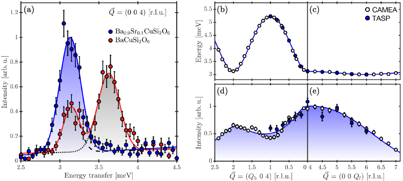
Figure 2: Inelastic neutron scattering analysis. (a) Scattered intensity as a function of energy transfer, measured on TASP at ${\vec{Q}}=(0\;0\;4)$ r.l.u. for Ba_0.9Sr_0.1CuSi₂O₆ at 1.5 K (blue symbols) and BaCuSi₂O₆ at 1.6 K (red). Shaded regions represent Gaussian fits used to extract the triplon energy, linewidth, and intensity. (b)-(e) Multiple Ba_0.9Sr_0.1CuSi₂O₆ energy scans, of the type shown in panel (a), were analyzed for ${\vec{Q}}$-vectors covering two high-symmetry directions in reciprocal space. (b)-(c) Triplon mode energies obtained from data gathered on TASP (blue symbols) and CAMEA (open). (d)-(e) Corresponding scattered intensities. Solid lines are fits obtained from the spin Hamiltonian represented in Fig. 1(b) with the optimal parameters given in the text.

The structure of our contribution is as follows. In Sec. II we detail our crystal-growth procedures, experimental methods, and numerical simulations. In Sec. III we report INS experiments at zero magnetic field, which demonstrate that this compound contains only one type of dimer bilayer, and hence one triplon excitation branch. We determine the minimal spin Hamiltonian, showing that it contains only the three Heisenberg interactions of Fig. 1(b), which form a clear hierarchy of intradimer ($J$), intra-bilayer ($J^{\prime}$), and inter-bilayer ($J^{\prime\prime}$) coupling strengths. Turning to high magnetic fields, in Sec. IV we perform magnetization, magnetic torque, specific-heat, magnetocaloric effect (MCE), and nuclear magnetic resonance (NMR) measurements to obtain a comprehensive experimental picture of the field-temperature phase boundary to the magnetically ordered state. In Sec. V we combine state-of-the-art statistical data analysis and Quantum Monte Carlo (QMC) simulations based on the INS parameters to interpret our results as demonstrating complete consistency with 3D scaling in the quantum critical region. In Sec. VI we discuss the context of these results, particularly regarding possible magnetic disorder effects, and conclude in Sec. VII that the structural consequences of weak chemical substitution by non-magnetic ions are sufficient to realize the simplicity and elegance of the model originally envisaged for Han Purple, namely a quasi-2D spin-dimer material displaying observable 3D quantum critical behavior.

II Material and Methods

II.1 Crystal growth

Single-crystal growth of BaCuSi₂O₆ poses a challenge because the starting CuO component decays before the reagents and compound melt. This decay has been suppressed by increasing the oxygen partial pressure in optical floating-zone growth Jaime2004 and by using oxygen-donating LiBO₂ flux Sebastian2006. However, the latter method cannot be applied to the substituted system, Ba_0.9Sr_0.1CuSi₂O₆, because the metaborate flux reacts with the SrO reagent Well2016. Thus two methods were employed to grow the single crystals used in the present work. All of the high-field experiments were performed using small single crystals (sizes of order 10 mg) grown from the congruent melt in a tube furnace with an oxygen flow at a pressure under 1 bar Well2016. The INS experiments were performed using one rod-shaped single crystal of mass 1.3 g grown by a floating-zone method. While this method was developed Puphal2019 for BaCuSi₂O₆, it could not be applied directly to Ba_0.9Sr_0.1CuSi₂O₆ because large oxygen bubbles from the reduction of CuO disconnected the two rods and terminated the crystal growth. In this sense, obtaining several gram-sized single crystals of Ba_0.9Sr_0.1CuSi₂O₆ constituted a significant achievement, made possible by using one single-crystalline seed in a mixed argon/oxygen atmosphere to reduce the sizes of the disruptive oxygen bubbles.

II.2 Inelastic neutron scattering measurements

INS measurements at zero applied magnetic field were performed on the triple-axis spectrometers TASP and on the multiplexing triple-axis spectrometer CAMEA Groitl2016; Lass2021, both at the SINQ neutron source Blau2009 at the Paul Scherrer Institute. INS probes the dynamical magnetic structure factor, $S({\vec{Q}},\omega)$, which is the spatial and temporal Fourier transform of the spin-spin correlation function, allowing direct access to the magnetic excitation spectrum as a function of the energy ($\hbar\omega$) and momentum ($\vec{Q}$) transfer of the scattered neutrons Furrer2009. On TASP, a temperature of 1.5 K was used and the final neutron energy was fixed to 3.5 meV. The instrumental parameters of a previous study of BaCuSi₂O₆ Allenspach2020 were selected to optimize the energy resolution. On CAMEA, a temperature of 1.5 K was used and sequential measurements at fixed incident neutron energies of 7.5 and 9 meV were combined to obtain a map of the spectrum over multiple Brillouin zones and over an energy range from 2.5 to 5.5 meV. For both measurements, the rod-shaped single crystal was aligned with ($h$ 0 $l$) in the scattering plane [notation from the crystallographic unit cell, Fig. 1(c)] Puphal2016.

The CAMEA data shown in Figs. 1(c)-1(f) were extracted from the raw measured intensities using the software MJOLNIR Lass2020, which corrects these intensities using measurements on a standard vanadium sample. The two datasets shown in Fig. 2(a) differed by sample masses and counting times, which for the Ba_0.9Sr_0.1CuSi₂O₆ sample were measured for approximately 7.5 minutes per point, while the BaCuSi₂O₆ data were measured for approximately 15 minutes per point. The comparison was made by scaling the BaCuSi₂O₆ data so that the integrated intensity of all three modes matched the integrated intensity of the single mode observed in Ba_0.9Sr_0.1CuSi₂O₆.

II.3 High-field measurements

Magnetization. Magnetization measurements up to 50 T were carried out in a capacitor-driven short-pulse magnet at the NHMFL Pulsed Field Facility in Los Alamos using an extraction technique Detwiler2000. These measurements are subject to a strong reduction of the sample temperature in the changing magnetic field, which was calibrated by explicit MCE measurements.

Specific heat. The specific heat was measured with a heat-pulse technique inside a motor-generator-driven long-pulse magnet at the International MegaGauss Science Laboratory of the University of Tokyo Imajo2020. The experimental data points were collected during the flat-topped portion of the magnetic-field profiles created by feedback loop control Kohama2015; Imajo2020, at fields up to 37.8 T and temperatures down to 1 K.

Magnetic torque. Measurements of the magnetic torque were conducted in a 31 T resistive magnet at the NHMFL DC Field Facility in Tallahassee using a silicon-membrane cantilever manufactured by NanoSensors^TM and a ³He cryostat to reach temperatures down to 0.3 K. Torque measurements were made during constant-temperature field sweeps across the phase boundary. The temperature was fixed by maintaining a constant ³He pressure in the sample space; two field-calibrated sensors, one located close to the cantilever and the other at the sample holder, were used for a precise in situ monitoring of the temperature. The angle between the field and the crystallographic axes of the sample was estimated by rotation tests to be 10.5^∘.

Magnetocaloric effect (MCE). MCE measurements were performed in vacuum at temperatures down to 1 K at the International MegaGauss Science Laboratory of the University of Tokyo Kihara2013, and down to 0.4 K at the NHMFL in Los Alamos. In both experiments, the temperature was recorded during magnetic-field pulses up to 50 T using the response of a thin-film AuGe thermometer sputtered onto the sample surfaces. Under adiabatic vacuum conditions, the lines defined by $T(H)$ may be understood as isentropes. The sign of the temperature change is given by the Maxwell relation $(\partial Q/\partial H)/T=-(\partial M/\partial T)|_{H}$; the changes of sign in the gradient of the isentropes correspond to the maxima or minima in $M(T)$ that occur at the ordering transitions.

Nuclear Magnetic Resonance (NMR). ²⁹Si NMR measurements were performed in the field range 22-26 T using a resistive magnet at LNCMI. A 13 mg single-crystal sample (5$\times$1$\times$0.5 mm³) was placed in the mixing chamber of a ³He-⁴He dilution refrigerator with its $c$-axis oriented parallel to the applied field, ${\vec{H}}$. NMR spectra were taken by the spin-echo pulse sequence. In the quantum disordered phase, the spectra are relatively narrow and were covered fully in a single-frequency recording; inside the magnetically ordered phase, the spectra are broader and their reconstruction required several recordings taken at equally spaced frequency intervals, by summation of the individual Fourier transforms. The frequency ($\nu$) of the ²⁹Si spectra was measured relative to the reference $\nu_{0}/(\mu_{0}H)=\,^{29}\gamma=8.4577$ MHz/T. The magnitude of the applied field was calibrated using a metallic ²⁷Al reference placed in the same coil as the sample. The same ²⁷Al reference was also used to obtain a relative temperature calibration at temperatures below 1 K from the Boltzmann-factor dependence of the NMR signal intensity; this was then related to the values measured directly by the field-calibrated RuO₂ temperature sensor at all higher temperatures, where stable and field-independent $T$ values were ensured by fixing the pressure of the He bath.

II.4 Quantum Monte Carlo

We performed QMC simulations by applying the stochastic series expansion (SSE) algorithm Syljuasen2002 on 3D lattices of $L$$\times$$L\times$$L/2$ sites for $L=8$, 10, 12, …, 32. To reduce the computational cost we simulated an effective Hamiltonian of hard-core bosons Mila1998, where each site represents a dimer and each site boson a dimer triplon. The dispersion relation of these bosonic quasiparticles was chosen to match the triplon band determined by INS.

For each applied field, the critical temperature, $T_{c}$, was extracted from the finite-size scaling of the superfluid density, $\rho_{\rm sf}$, of the hard-core bosons (equivalent to the spin stiffness of an ordered magnet). The quantity $L^{d+z-2}\rho_{\rm sf}(L,T)$ has scaling dimension zero, where the dimensionality $d=3$ and the dynamical exponent $z=0$ for a finite-temperature transition, and hence the $L\rho_{\rm sf}(L,T)$ curves for all $L$ cross at the same point, which is $T=T_{c}$ Sandvik1998. We verified that the values of $T_{c}(H)$, and the associated uncertainties $\delta T_{c}(H)$, determined in this way were fully consistent with the critical exponent, $\nu=0.672$, expected for the correlation length Allenspach2020.

III Magnetic excitations at zero field

The first step in characterizing the magnetic excitations of Ba_0.9Sr_0.1CuSi₂O₆ was to succeed in growing gram-sized single crystals by the technique described in Sec. IIA. Figures 1(c) and 1(d) show the experimental neutron spectrum measured on CAMEA over multiple Brillouin zones for two high-symmetry directions, ($Q_{h}$ 0 4) and (0 0 $Q_{l}$), in reciprocal space. The spectrum along ($Q_{h}$ 0 4) displays one triplon mode with a periodicity of 2 in $Q_{h}$ and the spin gap (band minimum) at even values of $Q_{h}$ [Fig. 1(c)]; this single mode has a periodicity of 4 in $Q_{l}$ and the spin gap appears at $Q_{l}=2+4n$ [Fig. 1(d)], where $n$ is an integer. In our model of the spectrum, shown in Figs. 1(e) and 1(f), one may state at the qualitative level that the location of the band minimum in $Q_{h}$ is a consequence of an effectively ferromagnetic (FM) intra-bilayer interaction parameter [$J^{\prime}$ in Fig. 1(b)], as proposed Mazurenko2014 and observed Allenspach2020 in BaCuSi₂O₆. Similarly, the location of the band minimum in $Q_{l}$ is a consequence of a FM inter-bilayer interaction parameter, $J^{\prime\prime}$, which is the magnetic coupling between the top ions of dimers in one bilayer and the bottom ions of the dimers in the next [Fig. 1(b)]. We remind the reader that the FM intra-bilayer correlations ensure that the inter-bilayer interactions are not frustrated for either sign of this latter parameter, excluding Mazurenko2014 the “dimensional reduction” scenario mentioned above. The leading qualitative feature of the intensities is the modulation visible in Figs. 1(c) and 1(e), which is a consequence of the fact that the resolution ellipsoid on CAMEA causes intensity to be spread over a narrower (focusing) or wider (de-focusing) range depending on the value of $\vec{Q}$.

Turning to a quantitative analysis of the low-temperature spectrum, Fig. 2(a) shows the scattered intensity as a function of energy transfer for Ba_0.9Sr_0.1CuSi₂O₆ (blue symbols), and also the comparison with BaCuSi₂O₆ (red) Allenspach2020, which we discuss in Sec. IIIB; both data sets were measured on TASP at ${\vec{Q}}=(0\;0\;4)$ using similar experimental conditions. The solid lines are Gaussian fits used to extract the location, linewidth, and intensity of the triplon modes. The results of applying the same procedure at all ${\vec{Q}}$ points along the same two high-symmetry directions as in Figs. 1(c)-1(f) are shown as the solid symbols in Figs. 2(b)-2(e), where the locations and intensities are compared to the analogous results obtained from CAMEA. The triplon dispersion relations measured on the two spectrometers are in excellent agreement throughout the Brillouin zone [Figs. 2(b) and 2(c)] and the measured intensities are fully compatible [Figs. 2(d) and 2(e)].

III.1 Spin Hamiltonian

We stress that our observation of one triplon mode per minimal magnetic unit cell means that the Ba_0.9Sr_0.1CuSi₂O₆ structure contains only one type of bilayer, in contrast to the complicated situation in BaCuSi₂O₆ Allenspach2020. An accurate determination of the spin Hamiltonian is crucial to verify the quasi-2D characteristics of the material and for a detailed investigation of the resulting critical behavior in an applied magnetic field. We assume that the minimal magnetic Hamiltonian of Ba_0.9Sr_0.1CuSi₂O₆ is that displayed in Fig. 1(b), i.e. that it contains only three interactions, all of purely Heisenberg type, to which, as above, we refer as intradimer ($J$), intra-bilayer ($J^{\prime}$), and inter-bilayer ($J^{\prime\prime}$). We note that $J^{\prime}$ is an effective inter-dimer interaction parameter that combines two pairs of ionic (Cu²⁺-Cu²⁺) interactions within and between the two layers of the bilayer structure Mazurenko2014; Allenspach2020.

By fitting the dispersion of the triplon mode shown in Figs. 2(b) and 2(c) as detailed in App. A, we deduce the optimal parameter set $J=4.28(2)$ meV, $J^{\prime}=-0.52(1)$ meV, and $J^{\prime\prime}=-0.02(1)$ meV, where negative values denote FM interactions and the error bars represent a conservative estimate of the statistical uncertainties. Figures 1(e), 1(f), and 2(b)-2(e) make clear that these parameters provide an excellent account of all the measured data, leaving no evidence of any requirement for further terms in the spin Hamiltonian. The INS parameters also serve as a benchmark for the magnetic interactions estimated using electronic structure calculations based on measurements of the atomic structure Puphal2016, from which one may deduce (using the notation in Table II of that work) that $J_{1}\equiv J$ is obtained to very high accuracy, $J_{3}-J_{5}\equiv J^{\prime}$ is overestimated by approximately 30%, $J_{4}=0$ is identified correctly, and $J_{2}\equiv J^{\prime\prime}$ is surprisingly accurate in both size and sign, given its small value. On this point, we stress that the three terms we have deduced form a hierarchy of interactions whose strengths differ by at least an order of magnitude, and hence that each is responsible for physics at quite different energy scales. Specifically, from the standpoint of triplon excitations, Ba_0.9Sr_0.1CuSi₂O₆ is very much a quasi-2D magnetic material, with an inter-bilayer coupling 25 times smaller than the energy scale characterizing the intra-bilayer excitation processes.

III.2 Comparison to BaCuSi₂O₆

It is instructive to compare the magnetic interactions of the Ba_0.9Sr_0.1CuSi₂O₆ system with those of the parent compound. The transition to a weakly orthorhombic structure below 90 K Samulon2006; Sparta2006; Stern2014 in BaCuSi₂O₆ results in the formation of three structurally inequivalent bilayers of dimers Rueegg2007; Sheptyakov2012. This led to the observation in INS experiments on BaCuSi₂O₆ of either three separate triplon modes or two separate peaks at ${\vec{Q}}$ vectors where the energies of the upper two modes are not distinguishable, which is the case in the data shown in Fig. 2(a) for ${\vec{Q}}=(0\;0\;4)$.

In Ba_0.9Sr_0.1CuSi₂O₆, the absence of this structural transition Puphal2016 means that the system remains tetragonal at low temperatures and only one bilayer type, hosting only one triplon mode, is expected. The neutron spectra presented in Figs. 1(c)-1(f) and 2 confirm this situation. If the tetragonal interaction parameters are compared with the orthorhombic ones, $J=4.28(2)$ is similar to $J_{A}=4.275(2)$ meV, the weakest of the three intradimer couplings in BaCuSi₂O₆ Allenspach2020, which explains the coincidence of the Ba_0.9Sr_0.1CuSi₂O₆ triplon shown in Fig. 2(a) with the lower peak in the BaCuSi₂O₆ data. By contrast, $J^{\prime}=-0.52(1)$ for the tetragonal structure is not close to $J^{\prime}_{A}=-0.480(3)$ meV, but lies between the stronger interactions $J^{\prime}_{B}=-0.497(8)$ meV and $J^{\prime}_{C}=-0.57(1)$ meV found in the distorted structure. Finally, inter-bilayer interaction, $J^{\prime\prime}=-0.02(1)$ meV, is only half the size of the corresponding value in BaCuSi₂O₆, which indicates the extreme sensitivity of these superexchange paths to the smallest structural alterations. However, while the bandwidth of the triplon mode visible in Figs. 1(c), 1(e), and 2(b) is very similar to that in BaCuSi₂O₆, the bandwidth of the inter-bilayer dispersion [Figs. 1(d), 1(f), and 2(c)] is much larger than the almost flat modes observed in BaCuSi₂O₆ Allenspach2020. This is a consequence of the ABC bilayer stacking in BaCuSi₂O₆, by which the three different dimer types cause a dramatic reduction of the inter-bilayer triplon hopping probability.

In principle, valuable physical information is also contained in the line widths of the triplon modes observed in the two materials. Partial Sr substitution on the Ba sites should result in a degree of bond disorder, meaning a distribution in the values of the interaction parameters, which would act to broaden the triplon in Ba_0.9Sr_0.1CuSi₂O₆. Comparison with the A triplon in BaCuSi₂O₆, which lies at the same energy in Fig. 2(a), reveals that the Full Width at Half Maximum (FWHM) of the Gaussian characterizing the 10%-substituted material is 20% higher at ${\vec{Q}}=(0\;0\;4)$ [0.32(2) meV as opposed to 0.25(2) meV]. At ${\vec{Q}}=(1\;0\;4)$, however, the FWHM is essentially unchanged [0.30(2) meV as opposed to 0.29(4) meV, not shown]. A number of factors affect this comparison, including that the Sr-substituted crystal was subject to a grain reorientation during growth Puphal2019 and that the different shapes of the two crystals made it necessary to adjust the focusing slits for each case, affecting the experimental resolution. On the basis of these results, we are not able to discern a significant intrinsic broadening, due to bond disorder, from the extrinsic contributions to broadening, and thus we make only the qualitative statement that disorder effects on the magnetic properties arising from the weak structural disorder caused by Sr-substitution are small in Ba_0.9Sr_0.1CuSi₂O₆.

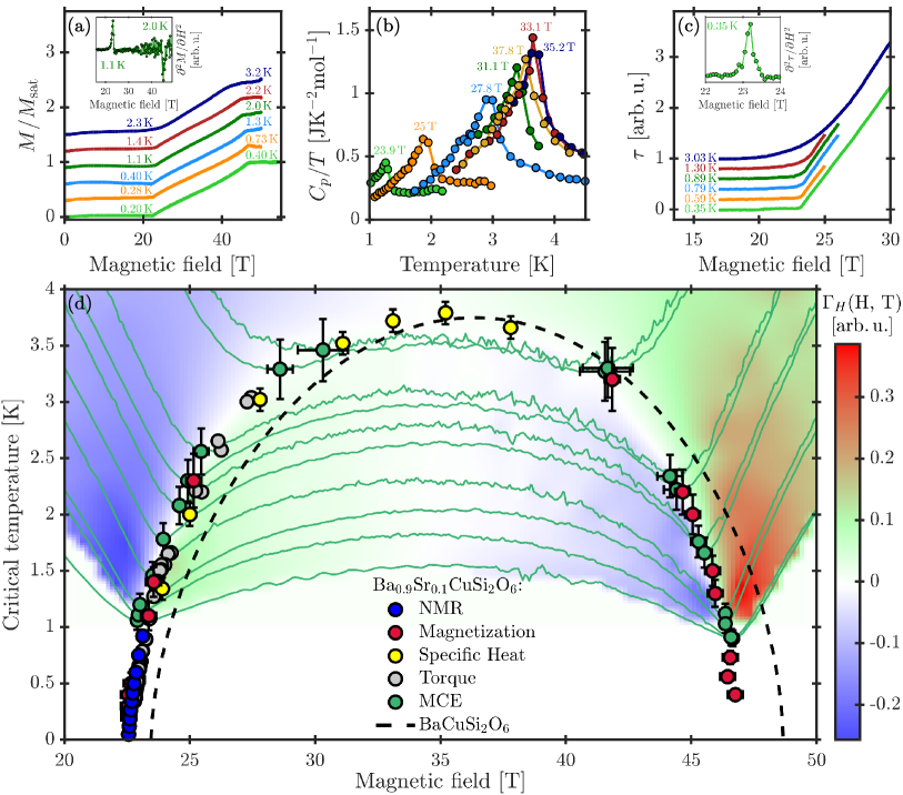
Figure 3: Phase boundary of Ba_0.9Sr_0.1CuSi₂O₆. Results from a wide range of thermodynamic measurements performed on single-crystalline Ba_0.9Sr_0.1CuSi₂O₆ at high magnetic fields, all with ${\hat{H}}\parallel{\hat{c}}$. (a) Magnetization, $M(H)$, measured in pulsed fields up to 50 T. Curves are shown with successive vertical offsets of 0.3. Left and right labels are the calibrated temperatures obtained respectively for the lower and upper phase transitions after correction for the strong magnetocaloric effects (MCEs) acting during the field pulse. The inset shows the second derivative, ${\partial^{2}M}/{\partial H}^{2}$, highlighting the locations of the ordering transitions. (b) Specific heat, $C_{p}(T)$, measured in pulsed fields up to 37.8 T and showing a $\lambda$-anomaly at the phase boundary. The maximum transition temperature, $T_{c}^{\rm max}\simeq 3.8$ K at 35.2 T, demarcates the top of the phase-boundary dome. (c) Magnetic torque, $\tau(H)$, measured in static fields around the onset of magnetic order. Curves above 0.35 K are shown with vertical offsets of 0.2. The inset shows the second derivative, ${\partial^{2}\tau}/{\partial H}^{2}$. (d) Field-temperature phase diagram of Ba_0.9Sr_0.1CuSi₂O₆ obtained by collecting all of our experimental data from magnetization, specific heat, magnetic torque, MCE, and NMR. Solid lines are lines of constant entropy obtained from our MCE measurements. Color contours represent the magnetic Grüneisen parameter, $\Gamma_{H}=-(\partial M/\partial T)/C_{p}=-(\partial T/\partial H)_{S}/T$, which shows a sharp change of sign at the phase boundary. The black dashed line shows for comparison the phase boundary of BaCuSi₂O₆ Jaime2004.

IV Field-temperature phase boundary

The parameters we have determined for the gapped, zero-field ground state have essential consequences for the field-temperature phase diagram. The onset of field-induced magnetic order, when the field is strong enough to close the triplon gap, is generally referred to as a Bose-Einstein condensation of magnons; while the quadratic magnon dispersion at the transition ensures the Bose-Einstein universality class, the effective dimensionality of the system remains an open issue, as explained in Sec. I. Given the questions raised by the parent compound BaCuSi₂O₆, and the more general questions raised about possible fingerprints of BKT physics in coupled quasi-2D systems Furuya2016, we have performed the most comprehensive study within our capabilities of the QPT and the surrounding quantum critical regime.

IV.1 High-field thermodynamic measurements

For this we applied a combination of thermodynamic measurements up to the highest available pulsed and static magnetic fields (Sec. IIC) to map the field-temperature phase diagram of Ba_0.9Sr_0.1CuSi₂O₆. Magnetization data obtained in pulsed fields are shown in Fig. 3(a). While zero magnetization indicates a spin gap, an abrupt jump and increasing $M(H)$ values are a signature of gap closure and magnetic polarization. The phase transitions both into and out of the ordered state are identified as sharp features in the second field derivative [inset, Fig. 3(a)]. Although field pulses up to 50 T make it possible to reach saturation even at the lowest temperatures, the $M(H)$ curves taken in short-pulse magnets are adiabatic, rather than isothermal. BaCuSi₂O₆ and Ba_0.9Sr_0.1CuSi₂O₆ have a strong MCE, meaning that the rapidly changing applied field drives a dramatic reduction of the sample temperature in the absence of heat transfer. We performed explicit MCE measurements (below) in order to obtain an accurate determination of the real measurement temperatures shown for both phase transitions in Fig. 3(a).

We have measured the specific heat in pulsed fields up to 37.8 T and display the results in Fig. 3(b). Because this field value is closer to the upper critical field of Ba_0.9Sr_0.1CuSi₂O₆ than to the lower, these measurements make it possible to access the top of the phase-boundary “dome” shown in Fig. 3(d). The $\lambda$-shaped anomalies in $C_{p}(T)$ are characteristic of second-order phase transitions and we used an equal-area method to estimate the critical temperatures for each magnetic field. The $\lambda$ shapes have also been associated directly with the 3D XY universality class in a number of systems showing magnon BEC Oosawa2001; Jaime2004; Sebastian2005; Aczel2009a; Aczel2009b; Kohama2011; Weickert2019, while below the transition $C_{p}(T)$ is consistent with the $T^{3}$ form expected from AF magnons in 3D.

In a static external field, we have measured the magnetic torque up to 29 T, as shown in Fig. 3(c). In these experiments the sample temperature is known exactly but, because a torque acts only when the sample is tilted away from its principal axes, the tilt angle provides a degree of uncertainty that affects the absolute field. By contrast, the relative values of the critical fields at each temperature are extremely accurate, allowing one to probe the shape of much of the left side of the phase-boundary dome. Again the second field-derivative [inset Fig. 3(c)] gives the most accurate determination of the critical field, $H_{c}$, for each measurement temperature, $T$. Here we have corrected these fields to the NMR values of $H_{c}(T)$ (below) in the regime of temperature where the two methods overlap, thereby obtaining the phase-boundary points shown up to 3.03 K in Fig. 3(d).

The MCE, meaning the change in sample temperature due to an applied field, is related directly to the first temperature derivative of the magnetization (Sec. IIC). MCE measurements in pulsed fields up to 50 T were used to obtain the lines of constant entropy shown in Fig. 3(d), whose local minima mark the location of the ordering transition in both field and temperature. We carried out two separate MCE experiments, at ISSP Tokyo and NHMFL Los Alamos, and used the latter data to deduce the true sample temperature for the magnetization results shown in Fig. 3(a). The MCE shows a discernible asymmetry [Fig. 3(d)], in that the phase-boundary temperature for the same isentrope is higher on the left side of the dome than on the right Nomura2020, indicating that the isothermal entropy, $S(H)$, is higher on the right than on the left. This result implies a larger specific heat on the right side of the dome and has been explained as a magnon mass anisotropy Kohama2011 that is connected to the ratio of the upper and lower critical fields. In Fig. 3(d) we show also the magnetic Grüneisen parameter, whose sign change becomes increasingly abrupt as the temperature is lowered, thereby locating the phase boundary with increasing accuracy.

We also performed NMR measurements at very low temperatures to determine the phase boundary close to the lower critical field, but defer a detailed discussion of these experiments to the next subsection. Figure 3(d) compiles all of our experimental data to display a comprehensive picture of the dome-shaped phase boundary of the magnetically ordered (condensate) phase. The dome is rather symmetrical in shape between a lower critical field $\mu_{0}H_{c1}\simeq 22.5$ T and an upper critical field $\mu_{0}H_{c2}\simeq 46.5$ T, with a maximum height of $T_{c}^{\rm max}\simeq 3.8$ K around 35 T. In Fig. 3(d) we show also the phase-boundary dome determined Jaime2004 for the parent compound, BaCuSi₂O₆, which is altered only slightly by the Sr substitution. Specifically, the small reduction of $H_{c1}$ is a consequence of the smaller gap in Ba_0.9Sr_0.1CuSi₂O₆, which arises due to the combination of increased bandwidth (controlled by $J^{\prime}$) and rather constant band center (controlled by $J$). The reduction of the upper critical field, $H_{c2}$, is a consequence of the fact that the stronger intra-dimer coupling constants of the structurally inequivalent bilayers in BaCuSi₂O₆ are absent in Ba_0.9Sr_0.1CuSi₂O₆.

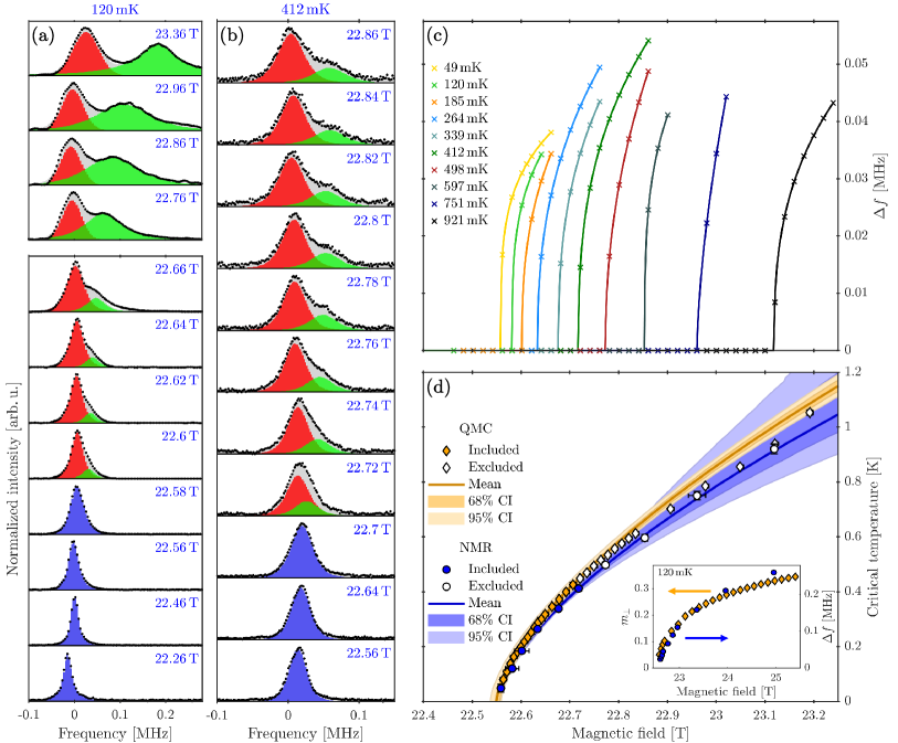
Figure 4: NMR measurements in the critical regime. (a)-(b) ²⁹Si NMR spectra measured for a range of field values around the corresponding value of $H_{c}(T)$ at 120 mK (a) and 412 mK (b). The spectra show a splitting from a single, sharp peak (blue) in the quantum disordered phase at $H<H_{c}(T)$ to two generally broader peaks (red and green) in the magnetically ordered phase at $H>H_{c}(T)$. The measured intensities were modelled as the sum (grey) of the single or double peak(s) and a weak, constant contribution. The double peaks were modelled by a simultaneous fitting procedure in all panels other than the highest four fields shown at 120 mK (a), where individual peak fits were used. (c) Splitting of peaks in the NMR spectra. Solid lines show splitting functions deduced from simultaneous fits to all spectra measured at the same temperature, and crosses mark the field values at which data were taken. (d) Low-field phase boundary of Ba_0.9Sr_0.1CuSi₂O₆ extracted from the NMR peak-splitting data (blue and white circles). Orange and white squares show the phase boundary obtained from QMC simulations. Blue and orange lines show the optimal fit to the phase boundary based on each set of points, obtained from the mean of the posterior distribution determined by a Bayesian inference procedure based on Eq. (1). The blue and orange shaded areas represent the estimated uncertainties in the form of the 68% (dark) and 95% (light shading) credible intervals (CIs). NMR and QMC data points marked by white circles and squares are those excluded from the statistical analysis of the quantum critical properties. Inset: NMR peak-splitting measured up to 25 T at $T=120$ mK (blue circles) juxtaposed with the magnetic order parameter, $m_{\perp}(T)$, obtained from QMC simulations.

IV.2 Nuclear Magnetic Resonance

For a detailed investigation of the quantum critical regime, we performed NMR measurements at high magnetic fields and very low temperatures using the facilities at the LNCMI (Sec. IIC). In the magnetically ordered phase above the critical field, which at any temperature we denote by $H_{c}(T)$, the presence of a staggered magnetization, $m_{\perp}(T)$, transverse to the direction of the external field (which is applied along the ${\hat{c}}$-axis) lifts the degeneracy between sites that were equivalent in the gapped dimer phase Berthier2017; Arcon2017. Their NMR spectra therefore show a splitting into two separate peaks. Figure 4(a) shows ²⁹Si NMR spectra obtained using a 13 mg single crystal of Ba_0.9Sr_0.1CuSi₂O₆ at $T=120$ mK over a range of static magnetic fields crossing the value of $H_{c}$ for this temperature. Whereas in BaCuSi₂O₆ it was possible by ²⁹Si NMR to detect only a broad distribution due to the presence of structurally different bilayer types Horvatic2005; Kraemer2007; Stern2014, whose local spin polarization could be determined quantitatively only by ⁶³Cu NMR Kraemer2013, in the ²⁹Si spectra of the Sr-substituted variant we observe a second peak that splits from the first with increasing applied field, becoming a separate and clearly resolved entity in the upper panels of Fig. 4(a).

Because of the low temperatures of these measurements, the field value at which the NMR peak-splitting appears constitutes our most accurate estimate of the critical field, $H_{c}(T)$, for each temperature, $T$, in the regime most likely to approach quantum critical scaling. The splitting of the peaks in frequency is directly proportional to the magnetic order parameter Berthier2017, allowing us to obtain the field-induced evolution of the ordered moment up to a single, non-universal constant of proportionality, which is the hyperfine coupling constant of the NMR experiment. To determine the field-dependence of the peak-splitting, and hence of the order parameter, we measured NMR spectra up to fields significantly higher than $H_{c}(T)$ for one example temperature, 120 mK [Fig. 4(a)], and the results are shown in the inset of Fig. 4(d). To determine the phase boundary for a study of its quantum critical properties, we have measured NMR spectra for a number of fixed temperatures between 49 and 921 mK, over a range of fields close to $H_{c}(T)$ in each case, and a further set of spectra is shown for $T=412$ mK in Fig. 4(b).

To optimize our extraction of the peak-splitting from the spectral data, which contain multiple additional features and complications, we exploit its relation to the order parameter to model it as a power-law function of the field difference from the phase transition, $H-H_{c}(T)$, and perform a simultaneous fit of one peak (blue) or two split peaks [red and green in Figs. 4(a) and 4(b)] to all NMR spectra measured at the same $T$. Details of this procedure, which is valid over a field-temperature regime near the phase boundary, are provided in App. B. Only at fields well above $H_{c}(T)$ was it possible to obtain reliable fits to the two clearly separated spectral peaks of each individual spectrum, and examples of these fits are shown in the upper panels of Fig. 4(a).

The result of the simultaneous fit procedure is the set of fitting functions shown by the lines in Fig. 4(c), where the crosses represent the fields at which spectra were collected, and these lines yield a set of estimated critical points, $H_{c,j}$, with uncertainties $\delta H_{c,j}$. The corresponding temperature values, with their uncertainties, were determined relative to a field-calibrated RuO₂ thermometer (Sec. IIC). The data pairs $(H_{c,j},\delta H_{c,j})$ and $(T_{c,j},\delta T_{c,j})$ together constitute the NMR phase boundary near the quantum critical point, which we show as the blue and open circles in Fig. 4(d). The blue line and shading represent the results of our statistical analysis of the quantum critical properties of the NMR phase boundary, which we discuss below.

To assist with the interpretation of the measured phase boundary, we performed large-scale QMC calculations of a model with only one type of bilayer, following the established procedure Allenspach2020 summarized in Sec. IID. For this we mapped the spin Hamiltonian of Fig. 1(b) to a hard-core-boson model Mila1998 for triplons with the low-energy triplon dispersion determined from our zero-field INS measurements. The QMC phase boundary in the regime close to the quantum critical point (QCP) is shown by the orange and open squares in Fig. 4(b), while the corresponding lines and shading are the results of the statistical analysis we present next (Sec. V). We remark that the precise agreement in location of the QCP obtained by using the zero-field parameters implies that magnetostriction effects are negligible, a result also found in BaCuSi₂O₆. We also performed QMC simulations to determine the order parameter at low temperatures for fields well inside the magnetically ordered regime, and in the inset of Fig. 4(d) these are shown for a temperature corresponding to 120 mK. By matching the field-induced ordered moment in Bohr magnetons to the peak-splitting measured in MHz over this field range, we obtain the hyperfine coupling constant as noted above.

V Critical exponent

From the statistical mechanics of classical phase transitions, the field-temperature phase boundary should be described by a power-law form in the critical regime close to the QCP, and hence can be expressed as

$$T_{c}(H)=\alpha\big{(}H-H_{c1}\big{)}^{\phi}.$$ (1)

Here $H_{c1}$ is the critical field of the QCP, i.e. at zero temperature, $\alpha$ is a nonuniversal constant of proportionality and $\phi$ is the critical exponent, which is universal and should reflect only the dimensionality of space and the symmetry of the order parameter. In a true BEC one has $\phi=2/d$ Nohadani2004; Kawashima2004; Sebastian2006; Laflorencie2009, where the numerator is the dynamical exponent for free bosons ($\omega\propto k^{2}$) and $d$ the dimensionality of space. The form of Eq. (1) means that the parameters ($\alpha$, $H_{c1}$, $\phi$) required to model the experimental data are highly correlated; specifically, the best estimate for $\phi$ depends strongly on the value of $H_{c1}$. Further, the width of the quantum critical regime, the ranges of $T_{c}$ and $H-H_{c1}$ over which Eq. (1) remains valid, is a non-universal quantity about which little specific information is available. Attempts to deal with both the correlation problem Sebastian2006 and the critical-regime problem Tanaka2001; Oosawa2002 on the basis of limited available data have led in the past to significant confusion, which has been cleared up for certain models Nohadani2004. In order to obtain an accurate estimate of $\phi$ and to quantify its uncertainty reliably, we have applied a thorough statistical analysis using Bayesian inference.

Bayesian inference is a general method for the statistical analysis of all forms of experimental data, and thus its applications can be found throughout physics Toussaint2011. The quantity of interest is the posterior probability distribution,

$$p(\bm{\theta}|\mathcal{D})\propto p(\mathcal{D}|\bm{\theta})p(\bm{\theta}),$$ (2)

of the model parameters, $\bm{\theta}$, conditional on the observed data, $\mathcal{D}$. In this expression of Bayes’ theorem, $p(\mathcal{D}|\bm{\theta})$ denotes the likelihood of making the observations $\mathcal{D}$ for a given $\bm{\theta}$ and $p(\bm{\theta})$ is a prior probability distribution summarizing any information previously available about the model parameters. In the problem of describing the phase boundary, $\bm{\theta}=(\alpha,H_{c1},\phi)$ is the set of parameters in the model of Eq. (1) and $\mathcal{D}=\{H_{c,j},T_{c,j},\delta H_{c,j},\delta T_{c,j}\}$ is the set of phase-boundary points with their associated uncertainties; clearly the total number of points ($j$) in the input information will have a leading role in determining the accuracy of the output. The posterior distribution, $p(\bm{\theta}|\mathcal{D})$, is a high-dimensional density function that contains all of the information available about the parameters in $\bm{\theta}$, including their uncertainties and (non-linear) correlations. To obtain individual parameter estimates and error bars, the posterior distribution is compressed in various ways. We use the mean of the marginal distribution of each parameter, which provides the prediction with the smallest error given the input data Toussaint2011. To quantify these errors, we construct the highest posterior-density credible intervals (CIs), which are the shortest intervals containing a fixed fraction of the posterior density Gelman2004, and show the commonly chosen 68% and 95% CIs.

Figure 4(d) shows the mean of the posterior distributions of the model function of Eq. (1) as a blue line for the NMR dataset, $\mathcal{D}_{\rm NMR}$, and an orange line for our QMC data, $\mathcal{D}_{\rm QMC}$, while the shaded regions indicate the 68% and 95% CIs. Referring back to the issue of the width of the quantum critical regime, the two posterior distributions were constructed on the basis of the 6 NMR phase-boundary data points falling below the temperature $T_{{\rm max}}^{{\rm NMR}}=412$ mK (blue circles) and the 17 QMC points below $T_{{\rm max}}^{{\rm QMC}}=426$ mK (orange squares). The criterion by which these maximum values were determined is discussed below, and an extension of the fit to higher temperatures is shown for reference.

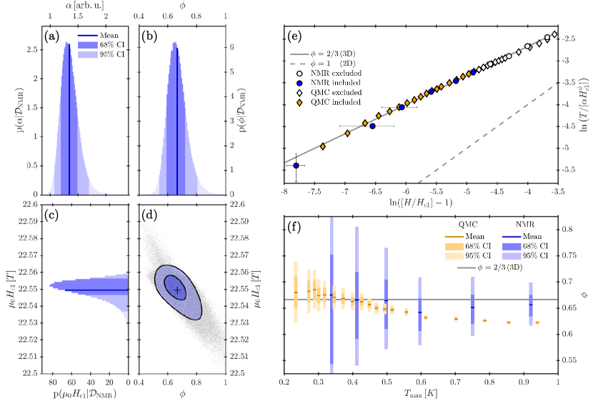
Figure 5: Analysis of the critical exponent. (a)-(c) Posterior probability distributions of the parameters in the model of Eq. (1) for the field-temperature phase boundary. The input for the analysis is the set, $\mathcal{D}_{\rm NMR}$, of 6 blue NMR data points up to $T_{\rm max}=412$ mK in Fig. 4(d). The marginal posterior distributions, $p(\theta_{i}|\mathcal{D})$, for each of the model parameters $\theta_{i}\equiv\alpha$ (a), $\phi$ (b), and $H_{c1}$ (c), are visualized as histograms of samples drawn from the posterior distribution together with their mean (blue lines), 68%, and 95% CI boundaries. (d) Posterior distribution shown by projection to $\phi$ and $H_{c1}$ (i.e. integrating over $\alpha$), which illustrates the strong negative correlation between the two parameters. (e) Phase-boundary points of Fig. 4(d) shown on logarithmic axes. The gradients of both sets of points correspond to the critical exponent, $\phi$. For comparison we indicate the cases $\phi=1$ (dotted) and $\phi=2/3$ (dashed lines). (f) Evolution of $\phi$ as a function of the maximal temperature, $T_{{\rm max}}$, up to which phase-boundary data points are included. Horizontal lines show the mean and shaded boxes the 68% and 95% CIs of the marginal distribution of $\phi$ deduced by including only points below $T_{\rm max}$; the 95% CIs for $T_{\rm max}=264$ mK lie at 0.465 and 0.923. The NMR symbols were obtained by including 5, 6, … 10 of the data points shown in Fig. 4(d) and panel (e), the QMC symbols by including between 8 and 30 data points.

To explain these results, Figs. 5(a)-5(c) show the marginal distributions, $p(\theta_{i}|\mathcal{D}_{\rm NMR})$, of each of the three model parameters in $\bm{\theta}$. These are normalized density distributions, obtained from Monte Carlo sampling of the posterior by integrating over the remaining two parameters in each case, which allow the full shape of each marginal to be investigated. These are clearly skewed, with the distributions of $\alpha$ [Fig. 5(a)] and $\phi$ [Fig. 5(b)] having tails extending towards larger values whereas that of $H_{c1}$ [Fig. 5(c)] extends towards smaller values. Qualitatively, the origin of these distorted shapes lies in the interplay of the uncertainties in the field and temperature measurements, whose simultaneous consideration is a key strength of the Bayesian approach; details of its quantitative implementation are presented in App. C. By contrast, a regression analysis such as a least-squares approach would yield biased estimates under these circumstances. Figure 5(d) shows a projection of the posterior distribution as a pair plot depending on $\phi$ and $H_{c1}$, which highlights the strong negative correlation between these two parameters. In the absence of accurate knowledge of $H_{c1}$, the NMR phase boundary data of Fig. 4(d) can often be described by decreasing $H_{c1}$ while simultaneously reducing the height of the curve, i.e. increasing $\phi$, or vice versa. In view of this situation, one may consider the precise goal of the present analysis as being to localize the most probable ($H_{c1}$, $\phi$) pair accurately on the axes of Fig. 5(d).

Using the mean and 68% CI boundaries of the marginal posterior distributions, from our NMR data for $T\leq T_{\rm max}^{\rm NMR}$ we obtain the model parameter estimates $\alpha=1.35^{+0.15}_{-0.16}$ K, $\mu_{0}H_{c1}=22.550^{+0.007}_{-0.003}$ T, and $\phi=0.666^{+0.053}_{-0.074}$. The non-universal parameter $\alpha$ has no influence on the critical properties. By comparing $H_{c1}$, for a field applied along the ${\hat{c}}$-axis, with the value of the spin gap extracted from INS, $\Delta=3.00(1)$ meV, we deduce a $g$-factor of $g_{\parallel c}=2.298^{+0.008}_{-0.008}$. This result is in agreement with both the value 2.32(2) determined for the Sr-doped material Puphal2016 and the value $g_{\parallel c}=2.306(3)$ obtained for the parent compound Zvyagin2006. Clearly the mean value of $\phi$ we obtain agrees spectacularly well with the 3D exponent of 2/3, although we stress that the CIs are broad (as one may expect from the number of data points in the analysis), and to interpret these results we turn to QMC modelling.

Because our QMC simulations were performed with an effective quasiparticle Hamiltonian matching the INS dispersion, $H_{c1}$ is fixed by the lower band edge (using the same $g$-factor) and the set of points $\{H_{c,j}\}$ has no errors ($\{\delta H_{c,j}\}=0$), which simplifies the statistical analysis (App. C). We deduce the values $\alpha={\rm 1.46}^{+0.03}_{-0.03}$ K and $\phi=0.663^{+0.008}_{-0.009}$, based on our data below $T_{{\rm max}}^{{\rm QMC}}=426$ mK. Figure 5(e) shows the putative critical regime on logarithmic axes, a format in which the gradient of each line is the critical exponent, $\phi$, and in which both our NMR and QMC results are indistinguishable from the line $\phi=2/3$ expected of a 3D BEC.

Returning to the width of the critical regime, this is a non-universal quantity in studies of critical behavior and hence is an unknown in any fitting procedure. Under these circumstances, the windowing fit was introduced Nohadani2004 to discern the trend of the data towards a critical value at the QCP when the width of the critical regime may be arbitrarily small, and has been applied Sebastian2006; Allenspach2020 for the analysis of BaCuSi₂O₆ data. To investigate this issue, we performed an effective windowing analysis by applying the Bayesian inference procedure using 10, 9, 8, 7, 6, and 5 NMR data points, and the results for the fitted exponents are shown as the blue symbols in Fig. 5(f). The horizontal lines show the mean and the heights of the shaded boxes show the 68% and 95% CIs of the marginal posterior distribution of $\phi$ for each case. We observe that the estimated mean value of $\phi$ is almost exactly 2/3 for the three narrowest windows, but then dips on inclusion of the 8th data point and recovers slightly towards 2/3 when the 9th and 10th points are considered. However, by a criterion that the mean $\phi$ should include 2/3 within the 68% CI, all of these windows are consistent with 3D critical scaling.

For further insight as to whether it is realistic to ascribe this behavior in its entirety to quantum critical physics, we perform the same type of analysis using our QMC data. While QMC studies of 3D models have revealed quantum critical regimes with relative widths on the order of 10-20% of the control parameter Nohadani2004; Qin2015, simulations of quasi-1D models have struggled to reach such a regime. Our QMC results, which have better data coverage and much narrower CIs, can be expected to reflect the physics of quasi-2D bosons at the energy scales of their interlayer coupling. The data in Figs. 5(f) show a systematic and near-monotonic evolution best described as the estimated $\phi$ converging to 2/3 from below as the number of data points is reduced. If one defines $T_{\rm max}$ as the highest temperature at which $\phi$ has converged to 2/3 within the 68% CI, one obtains $T_{\rm max}^{{\rm QMC}}=426$ mK, which corresponds to the use of 17 phase-boundary points. On this basis we deduce that effects beyond quantum critical fluctuations become discernible above approximately 0.4 K, and hence that this is an appropriate width to adopt for the scaling regime.

This criterion terminates our NMR dataset at $T_{\rm max}^{\rm NMR}=412$ mK, corresponding to the 6 phase-boundary points used for the analysis shown in Figs. 4(d) and 5(a)-5(d). However, we note that the criterion is far from exact, and in the present case an almost identical estimate with lower uncertainties, $\phi=0.665^{+0.040}_{-0.054}$, is obtained by including the 7th data point. The evolution of the estimated $\phi$ on inclusion of the 9th and 10th data points indicates both the onset of complex and manifestly non-monotonic crossover behavior beyond the critical regime and the accuracy of the analysis beyond features visible in Figs. 4(d) or Figs. 5(e). The discrepancy between the forms of behavior exhibited by our NMR and QMC data could lie in interaction terms neglected in our minimal magnetic Hamiltonian, or in possible disorder effects arising due to Sr substitution, which we discuss further in Sec. VI. However, we stress that these differences in critical behavior are extremely subtle, and are certainly not discernible in the NMR and QMC phase boundaries shown in Fig. 4(d).

To summarize, our NMR measurements and statistical analysis, backed up by our QMC simulations, present a quite unambiguous demonstration of 3D critical physics in a material with a strongly quasi-2D structure and magnetic properties. With reference to the prediction that unconventional magnetic ordering bearing the hallmarks of BKT physics should appear uniquely in 3D coupled quasi-2D systems Furuya2016, our results [Figs. 3(c) and 4(d)] demonstrate that the field-induced onset and evolution of the ordered phase are quite conventional. From this we conclude that the inter-bilayer coupling in Ba_0.9Sr_0.1CuSi₂O₆ is still significantly too large to access BKT physics, despite being only 1/100 of the magnon bandwidth (1/25 of the intra-bilayer interaction, a value that by any other measure appears worthy of the designation “quasi-2D”). Nevertheless, the restoration of observable 3D quantum criticality from an apparently minor chemical substitution constitutes a somewhat remarkable consequence of structural “disorder.”

VI Discussion

We have found that the interaction parameters of Ba_0.9Sr_0.1CuSi₂O₆ determined by INS at zero field, $J=4.28(2)$ meV, $J^{\prime}=-0.52(1)$ meV, and $J^{\prime\prime}=-0.02(1)$ meV, provide an excellent description not only of the triplon spectrum (Figs. 1 and 2) but also of the critical properties at the field-induced QPT [Figs. 4(d) and 5]. It is notable that these interaction parameters are not changed, within the error bars of our zero- and high-field experiments, by applied fields in excess of 20 T. More noteworthy still is the hierarchy of energy scales contained within the minimal spin Hamiltonian, which appear to define a quasi-2D material. The zero-field spectrum measured in Figs. 1 and 2 probes largely the intra-bilayer energy scale, which gives the triplons a bandwidth of 2 meV. However, it is clear in Fig. 5(f) that the inter-bilayer energy of fractions of a Kelvin is the scale on which the 3D physics emerges.

We remark again that the FM effective intra-bilayer interaction removes any frustration of the inter-bilayer interactions, reinforcing the expectation of a simple scaling form around the QCP. In a windowing analysis of the critical scaling in BaCuSi₂O₆, an abrupt change in behavior towards an exponent $\phi=1$ was reported below 0.75 K, which was interpreted as a frustration-induced dimensional reduction Sebastian2006. Subsequent investigation has revealed the absence of frustration Mazurenko2014, the presence of structurally inequivalent bilayers Rueegg2007; Sheptyakov2012, and the problem of the strong negative correlation between $\phi$ and $H_{c1}$ [shown clearly in our Fig. 5(d)]. The experimental confirmation of the absence of frustration was accompanied by detailed QMC simulations of the quantum critical regime, from which it was possible to conclude that the true behavior of the system includes an intermediate field-temperature regime of non-universal scaling governed by an anomalous exponent whose value turned out to be $\phi\gtrsim 0.72$ over much of the effective scaling range Allenspach2020. This result raises the question of whether our present analysis, which obviously relies on a limited number of experimental data points, can be regarded as sufficiently precise to claim that Ba_0.9Sr_0.1CuSi₂O₆ shows true 3D scaling. For this we appeal first to the fact we demonstrated by INS, that the Sr-substituted material has only one bilayer type and one species of triplon (Figs. 1 and 2), whereas all the complications leading to anomalous scaling in BaCuSi₂O₆ result from a new effective energy scale dictated by the separation of the inequivalent triplon modes. Thus in the Sr-substituted case one expects both a wider critical regime and a lack of alternatives other than the universal 2D or 3D forms, and our results are certainly not consistent with 2D scaling ($\phi=1$). Second, we note from the error bars in the QMC data for the layered model of BaCuSi₂O₆ Allenspach2020 that the anomalous effective exponent is in no way compatible with 2/3; by contrast, our NMR data for Ba_0.9Sr_0.1CuSi₂O₆ favor strongly an exponent of 2/3 in Fig. 5(f) rather than any anomalous value, as do our QMC simulations for the model with only one type of bilayer.

The crux of our analysis is the materials-synthesis result that Sr substitution improves the regularity of the BaCuSi₂O₆ structure, maintaining tetragonal symmetry and eliminating the orthorhomic transition that also produces the structurally inequivalent dimer bilayers. However, the introduction of the smaller Sr ion in the inter-bilayer position of the Ba ions also creates a local strain most likely to act along the ${\hat{c}}$-axis within the bilayers. The most important statement concerning any magnetic disorder produced by this structural disorder is that it can be at most a bond disorder, and not a site disorder, because the Cu²⁺ sites are unaffected. Because of the inter-bilayer location of the Ba²⁺ and Sr²⁺ ions, this bond disorder is most likely to affect the local value of $J^{\prime\prime}$, a parameter so small that our results are not very sensitive to the possibility of a distribution of values. The most important observation in the context of possible magnetic disorder is the result of our INS measurements that any resulting triplon broadening (lifetime) effects are too small to be distinguished from extrinsic factors (Sec. IIIB). From this we may conclude that local magnetic effects arising from this disorder are minimal, and that it has no discernible consequences for the magnetic Hamiltonian. Thus the disorder can be called “ideal” in the sense that only its qualitative and quantitative effects on the average structure are relevant. Regarding its density, while the nominal substitution was $x=0.1$ and a compatible value of $x=0.08(2)$ was determined by energy-dispersive x-ray spectroscopy (EDX), a somewhat lower value of $x=0.05(1)$ was obtained from Rietveld refinement of synchrotron diffraction data for crushed crystals Puphal2016.

Further disorder effects within our experiment are the following. The density of magnetic impurities was estimated by fitting the Curie tail in the magnetic susceptibility, which arises at the lowest temperatures due to free spin-1/2 levels, and was found to be 3% in the best crystals selected for our experiments Puphal2016; Puphal2019. A typical nonmagnetic impurity in BaCuSi₂O₆ is Cu₂O, which can be created by the decay of CuO during crystal growth; it is visible on surfaces and in thinner crystals, allowing its presence to be minimized by careful selection of crystals. In our INS experiments, the floating-zone-grown single crystals have a reorientation in growth direction of up to 15^∘ as a consequence of the growth process Puphal2019. However, it is important to stress that none of these possible sources and consequences of disorder are significant when compared to the complex and incommensurate crystal structure and magnetic Hamiltonian realized in the parent material Samulon2006; Rueegg2007; Kraemer2007; Sheptyakov2012; Allenspach2020.

VII Conclusion

In summary, we have performed a comprehensive experimental and numerical analysis of the quasi-2D dimerized antiferromagnet Ba_0.9Sr_0.1CuSi₂O₆. The non-magnetic site disorder due to this weak Sr-substitution of Han Purple affects only the lattice, acting to stabilize the tetragonal room-temperature structure of the parent material down to the lowest temperatures. We have measured the spin excitation spectrum at 1.5 K and zero applied magnetic field to verify that indeed there is only one triplon branch, and hence that all dimer bilayers are structurally and magnetically equivalent in this compound. This triplon has a spin gap of 3.00 meV and is described by only three Heisenberg superexchange interactions, all on very different energy scales.

To examine the consequences of these interactions for field-induced magnetism and universal critical properties at the magnetic transition, we have gathered extensive thermodynamic data at high fields and low temperatures using a range of experimental techniques, including a detailed NMR study of the quantum critical phase boundary. For an optimal analysis of these latter data, we have performed Bayesian inference to obtain the critical exponent $\phi=0.67^{+0.05}_{-0.07}$, determined by assuming a quantum critical regime of approximate width 0.4 K. QMC simulations of a 3D model with a single type of bilayer yielding the triplon band determined from the zero-field INS measurements provide excellent agreement with the quantum critical phase boundary, return a critical exponent $\phi=0.66^{+0.01}_{-0.01}$, and indicate both a convergence to $\phi=2/3$ and the actual width of the regime over which this quantum critical scaling is obeyed. We conclude that the structural alteration caused by the small chemical modification of Han Purple to its 10% Sr-substituted variant fully restores the originally envisaged properties of 3D quantum critical scaling at the field-induced magnetic ordering transition of a structurally and magnetically quasi-2D system.

Appendix A Neutron spectrum calculations

The single-particle excitations in an AF spin-dimer material with a global singlet ground state are coherently propagating triplets, commonly referred to as triplons. To determine the interaction parameters of Ba_0.9Sr_0.1CuSi₂O₆, we have modelled the magnetic dynamical structure factor, $S(\vec{Q},\omega)$, by applying a triplon-based RPA approach Leuenberger1984; Allenspach2020. In this framework, the zero-temperature dispersion of the single triplon mode is given by

$$\omega(\vec{Q})=\sqrt{J^{2}+JJ(\vec{Q})}$$ (3)

for $\vec{Q}\equiv(Q_{h},Q_{k},Q_{l})$ in the crystallographic basis, with

$$J(\vec{Q})= 2J^{\prime}\big{[}\cos(\pi[Q_{h}+Q_{k}])+\cos(\pi[Q_{h}-Q_{k}])\big{]}$$ (4)

$$-2J^{\prime\prime}\cos({\textstyle\frac{1}{2}}\pi Q_{l})\big{[}\cos(\pi Q_{h})+\cos(\pi Q_{k})\big{]}.$$ (5)

The INS intensities, $I(\vec{Q},\omega)$, are given by

$$I(\vec{Q},\omega)=\mathcal{A}F^{2}_{\rm{mag}}(\vec{Q})S(\vec{Q},\omega),$$ (6)

where $\mathcal{A}$ is an overall prefactor. The magnetic form factor, $F_{\rm{mag}}(\vec{Q})$, is known to be spatially anisotropic Allenspach2020 and hence was modelled using the minimal parametrization

$$F_{\rm{mag}}(\vec{Q})\!=\!C_{1}e^{-(c_{h1}Q_{h}^{2}+c_{l1}Q_{l}^{2})}\!+\!C_{2}e^{-(c_{h2}Q_{h}^{2}+c_{l2}Q_{l}^{2})}.$$ (7)

Theoretically, the dynamical structure factor at zero temperature due to the triplon is given by

$$S(\vec{Q},\omega)=N\big{[}1-\cos(\vec{Q}\!\cdot\!\vec{R})\big{]}\frac{J}{\omega(\vec{Q}\,)}\delta\big{(}\omega(\vec{Q})-\omega\big{)},$$ (8)

where $N$ is the number of dimers in the crystal and $\vec{R}$ the vector connecting the two ions of a single dimer. In experiment, $N$ is absorbed in $\mathcal{A}$ and the $\delta$-function is replaced by a Gaussian of unit integrated intensity and width $\Gamma(\vec{Q})$, which includes both intrinsic dynamical and extrinsic instrumental resolution effects. In the modelled spectra shown in Figs. 1 and 2, $\Gamma(\vec{Q})$ was fitted separately at every $\vec{Q}$ point. $\mathcal{A}$ and $F^{2}_{\rm{mag}}(\vec{Q})$ were fitted using the intensity data shown in Figs. 2(d) and 2(e) while keeping the interaction parameters fixed to their optimal values determined using the dispersion data of Figs. 2(b) and 2(c).

Appendix B Extraction of NMR phase boundary

To extract the phase boundary of Ba_0.9Sr_0.1CuSi₂O₆ from the NMR spectra, we modelled the opening and increase of the peak-splitting visible in Figs. 4(a) and 4(b) by exploiting its direct proportionality to the order parameter [inset, Fig. 4(d)]. In the critical regime we therefore assumed that the splitting of peak frequencies is given by

$$\Delta f(H,T)=c(T)[H-H_{c}(T)]^{\zeta(T)}$$ (9)

for each measurement temperature, $T$. This allowed us to perform simultaneous fits of all spectra at each $T$, and hence to optimize the accuracy of our estimate for the corresponding $H_{c}(T)$.

To model the shapes of the NMR peaks [Figs. 4(a) and 4(b)] we used the Student $t$-distribution. A single peak was used below $H_{c}(T)$ and two peaks above, where $H_{c}(T)$ is the key parameter to be fitted. Implementing this behavior required a number of additional assumptions. The widths of the peaks below $H_{c}(T)$ [blue in Figs. 4(a) and 4(b)] and of the lower-frequency peaks above $H_{c}(T)$ (red) were treated as individual parameters, while the widths of the higher peaks above $H_{c}(T)$ (green) were parametrized using a low-order polynomial in order to avoid spurious contributions from background features. The shape parameters of the $t$-distributions were modelled using a function linear in $H-H_{c}(T)$, which allowed us to confirm that the shape remains almost constant for different fields. The relative intensity ratio of the two peaks, and the size of a constant background parameter, were taken to be the same for all spectra measured at the same temperature. To assist the fit convergence, and because the important parameter is the position or positions of the NMR peak(s), all integrated intensities were normalized to unity before processing.

Appendix C Bayesian analysis of phase-boundary data

To analyze the NMR and QMC data close to the QCP within the framework of Eq. (1), it is necessary to specify the functions entering Eq. (2). Beginning with QMC, the critical fields, $H_{c1}$ and $\{H_{c,j}\}$, are input values for the simulation and hence are known exactly ($\{\delta H_{c,j}\}=0$). The corresponding critical temperatures, $\{T_{c,j}\}$, are estimates based on extrapolation from repeated simulations with increasing grid sizes and we assumed them to obey a normal distribution around the true critical fields with standard deviations $\{\delta T_{c,j}\}$. The likelihood function was therefore taken to be

$$p(\mathcal{D}_{\rm QMC}|\bm{\theta}_{\rm QMC})=\prod_{j=1}^{j_{\mathrm{max}}}\mathcal{N}(T_{c,j}|\alpha[H_{c,j}-H_{c1}]^{\phi},\delta T_{c,j}),$$ (10)

where $\mathcal{N}(x|\mu,\sigma)$ denotes the probability density function of the normal distribution with mean $\mu$ and standard deviation $\sigma$, evaluated at $x$. In this expression $\bm{\theta}_{\rm QMC}\equiv(\alpha,\phi)$ contains only two unknowns and $j_{\rm max}$, the index of the data point with temperature $T_{c,j}=T_{\rm max}$, introduces the finite width of the quantum critical regime. The statistical relationship between the phase-boundary parameters and the observations in this case is therefore that of a regression model.

In the phase-boundary data obtained by NMR, both the critical fields and the corresponding temperatures are estimated quantities. Each temperature, $T_{c,j}$, is subject to both measurement uncertainties and possible systematic variations, and was treated as a noisy measurement of a single value. Each critical field, $H_{c,j}$, was obtained from the NMR peak-splitting with an uncertainty that arises from background, noise, and the finite number of measurements, as a result of which it is essentially uncorrelated with $\delta T_{c,j}$. The presence of uncertainty in two measurement dimensions means that the true point on the phase boundary at each $j$ is unknown. Its location can be parametrized by either a temperature or a field coordinate, and here we chose the latter, introducing the parameters $\{H_{c,j}^{*}\}$ to represent the true, unknown critical fields of which $\{H_{c,j}\}$ are uncertain estimates. Taking $\{H_{c,j}\}$ and $\{T_{c,j}\}$ to be independent and to have a normal distribution around these true phase-boundary points, with respective standard deviations $\{\delta H_{c,j}\}$ and $\{\delta T_{c,j}\}$, the likelihood function was taken as

$$p(\mathcal{D}_{\rm NMR}|\bm{\theta}_{\rm NMR}) = \prod_{j=1}^{j_{\mathrm{max}}}\mathcal{N}(T_{c,j}|\alpha[H_{c,j}^{*}-H_{c1}]^{\phi},\delta T_{c,j})$$ (11)

$$\;\;\;\;\;\;\;\;\;\;\times\mathcal{N}(H_{c,j}|H_{c,j}^{*},\delta H_{c,j}),$$

where $\bm{\theta}_{\rm NMR}$ denotes the extended parameter set $(\alpha,H_{c1},\phi,H_{c,j}^{*})$. In the Bayesian methodology, once the posterior is obtained its dependence on the introduced parameters $\{H_{c,j}^{*}\}$ can be removed in an optimal manner by averaging over all possible values weighted by their posterior probability.

Turning to the prior probability distributions in Eq. (2), their selection should guide the inference process efficiently without introducing undue bias in the final result. $\alpha$ is known from studies of BaCuSi₂O₆ Sebastian2006; Allenspach2020 only to be of order unity (for measurements in T and K), and hence we assigned it an uninformative normal distribution on a logarithmic scale. For $\mu_{0}H_{c1}$, we used the gap $\Delta=3.00(1)$ meV obtained from the INS data and the $g$-factor $g_{\parallel c}=2.32(2)$ Puphal2016 to obtain an initial estimate of $22.34\pm 0.24$ T. Because $\phi$ is positive and is not expected to exceed unity, we used as its prior a half-normal distribution, $\mathcal{N}_{\rm{half}}(x|\sigma)$, with the scale parameter chosen to ensure that it is approximately flat in the region where $\phi$ is physically plausible, but does permit larger values. These considerations gave the prior probability distributions

$$\begin{split}p(\log_{10}\alpha)&=\mathcal{N}(\log_{10}\alpha|0,3),\\ p(H_{c1})&=\mathcal{N}(\mu_{0}H_{c1}|22.34\leavevmode\nobreak\ {\rm T},0.24\leavevmode\nobreak\ {\rm T}),\\ p(\phi)&=\mathcal{N}_{\rm{half}}(\phi|2),\end{split}$$ (12)

for the three model parameters. For the true critical fields, $\{H_{c,j}^{*}\}$, required to analyze the NMR phase boundary, these are unknown before measurement and thus we assigned a flat prior probability distribution,

$$p(H_{c,j}^{*})=\mathcal{U}(\mu_{0}H_{c,j}^{*}|0\,\mathrm{T},50\,\mathrm{T}),$$ (13)

where $\mathcal{U}(x|a,b)$ denotes a uniform distribution with limits $a$ and $b$. We made the minimal assumption that the range of possible values does not exceed 0-50 T, which includes the entirety of the ordered phase. Because all of these probabilities are independent, the joint prior probability distributions, $p(\bm{\theta}_{\rm QMC})$ and $p(\bm{\theta}_{\rm NMR})$, entering Eq. (2) are given by their product.

To investigate the unknown width of the quantum critical regime, we repeated the analysis of our NMR data multiple times with $339\leavevmode\nobreak\ {\rm mK}\leq T_{\rm max}\leq 921\leavevmode\nobreak\ {\rm mK}$ ($5\leq j_{\rm max}\leq 10$ data points) and of our QMC data with $234\leavevmode\nobreak\ {\rm mK}\leq T_{\rm max}\leq 939\leavevmode\nobreak\ {\rm mK}$ ($8\leq j_{\rm max}\leq 30$ data points). In each case we recovered the posterior by drawing random samples using emcee ForemanMackey2013, a Markov-chain Monte Carlo implementation of an affine invariant ensemble sampler Goodman2010. An ensemble of 200 chains was sampled for 40 000 steps to ensure equilibration of the Markov process before a further 10 000 steps were recorded, yielding a total of 2 000 000 parameter samples for each $j_{\rm max}$. These samples form point clouds in the parameter space of $\bm{\theta}$, whose density is proportional to the posterior probability, and one of these (obtained using the NMR data with $j_{\rm max}=6$) is visualized using different projections in Figs. 5(a)-5(d). As a heuristic confirmation of convergence we note that the maximal autocorrelation time Goodman2010 was 117 steps. The posterior standard deviations are at least 20 times smaller than the prior ones in all cases, confirming that, after convergence, the results depend only on the data and not on our choice of weakly informative prior.