Real-time quantum calculations of phase shifts using wave packet time delays

Erik Gustafson

{}^{1}

Yingyue Zhu

{}^{2}

Patrick Dreher

{}^{3}

{}^{4}

Norbert M. Linke

{}^{2}

Y. Meurice

{}^{1}

{}^{1}

Department of Physics and Astronomy, The University of Iowa, Iowa City, IA 52242, USA

{}^{2}

Joint Quantum Institute and Department of Physics, University of Maryland, College Park 20740, USA

{}^{3}

Department of Computer Science, North Carolina State University, Raleigh, NC 27695, USA

{}^{4}

Department of Physics, North Carolina State University, Raleigh, NC 27695, USA

(March 12, 2024)

Abstract

We present a method to extract the phase shift of a scattering process using the real-time evolution in the early and intermediate stages of the collision in order to estimate the time delay of a wave packet. This procedure is convenient when using noisy quantum computers for which the asymptotic out-state behavior is unreachable. We demonstrate that the challenging Fourier transforms involved in the state preparation and measurements can be implemented in $1+1$ dimensions with current trapped ion devices and IBM quantum computers. We compare quantum computation of the time delays obtained in the one-particle quantum mechanics limit and the scalable quantum field theory formulation with accurate numerical results. We discuss the finite volume effects in the Wigner formula connecting time delays to phase shifts. The results reported involve two- and four-qubit calculations, and we discuss the possibility of larger scale computations in the near future.

1. Introduction. The idea of simulating quantum field theory with quantum computers has gained considerable interest recently PreskillPOS. In the context of high-energy and nuclear physics, a long term motivation is to develop quantum computing methods that perform real-time evolution for lattice quantum chromodynamics (QCD). This is an ab-initio, ultraviolet complete, theory of strong interactions which has been very successful in describing the static properties of hadrons and nuclei ¹¹1See review 17 of the PDG pdg.. Importance sampling methods, used successfully today for lattice QCD at Euclidean time, are not effective for dealing with the rapid oscillations of real-time unitary operators acting on large Hilbert spaces. Currently, physicists resort to semi-empirical algorithms such as Pythia and Herwig pythiamanual; HerwigManual) to interpret hadronic collider data. Doing ab-initio calculations for jet physics would represent a major accomplishment and remains a long-term goal for the high-energy community and strategies to deal with parton distributions are outlined in Refs. PhysRevD.102.016007; Lamm_2020. Related methods for out-of-equilibrium processes in many-electron systems and information paradoxes in quantum gravity PreskillMicrosoft would also have a large potential impact.

Quantum computers offer an alternative solution to the sign problem plaguing current efforts. A sensible approach would be to follow the sequence of models that has been successful for the development of lattice QCD at Euclidean time on classical computers RevModPhys.51.659; RevModPhys.55.775. The first step in this sequence is to study and understand the properties and behavior of the quantum Ising model (QIM) on today’s Noisy Intermediate-Scale Quantum (NISQ) hardware.

Real time evolution involving a limited number of sites for the QIM has already been attempted using a few qubits on gate based quantum computers CerveraLierta2018exactisingmodel; Lamm:2018siq; GustafsonIsing; gustafson2019real; Kim_2020; yeteraydeniz2021scattering; vovrosh2020confinement; Kandala:2017aa; Kandala_2019; Salath__2015; Labuhn_2016; 2017Natur.551..601Z; PhysRevE.58.5355; 2017Natur.551..579B, as well as developments in progress for more complicated models Alexandru_2019; Zohar_2013; Martinez_2016; Klco:2018kyo; brower2020lattice. Today researchers must grapple with discrepancies between the measured qubit-state occupations on quantum platforms and the exact evolution after only a few Trotter steps. Currently, error-mitigation methods such as zero-point extrapolation Richardson; Klco:2018kyo are necessary to improve the computational results. It has been shown gustafson2019real that by modelling four qubits on an IBM Q quantum computing hardware platform these mitigation methods provide a reasonable extrapolation for times of the order of the approximate periodicity of the problems considered. It is possible to use Trotter steps that are more than 20 times larger than rigorous bounds in $(\delta t)^{2}$ or $(\delta t)^{3}$ would naively suggest, without encountering major discretization errors gustafson2019real; ybook. This allows us to reach larger time scales for studying scattering processes.

Refer to caption — Figure 1: Illustration of the measurement of the time delay between the free and interacting wave packets. The renormalized reflection probability $R_{-}(t)$ is defined in Eq. (13)

In this Letter, we demonstrate that it is possible to use state-of-the-art NISQ devices to prepare and evolve suitable wave packets for the QIM. We show that it is possible to project the wave-function in the early stages of a collision process onto momentum states and to pinpoint a time that corresponds to the middle of the collision. By introducing an extra interaction, we obtain a time delay $\Delta t^{\star}$ illustrated in Fig. 1 that is half of the time delay $\Delta t_{W}$ invoked in Wigner formula PhysRev.98.145 given in Eq. (6) to estimate the derivative of the phase shift with respect to the momentum.

Phase shifts are a key measurement in the scattering process and represent the total change of phase due to interactions. Significant progress has been made in calculating them from lattice QCD in Euclidean time Luscher1986; Briceno:2013bda; Briceno:2016mjc; Briceno:2017max; SavageLAT2016; Davoudi:2018wgb. In standard textbooks, phase shifts and scattering amplitudes are estimated from asymptotic data long after the collision processes have occurred. However, for NISQ devices with limited coherence time or gate-depth, using the information from the early stages of the collision is advantageous. We show that this idea can be implemented on both a quantum computer using superconducting transmon qubits and a trapped ion system operating at the University of Maryland Debnath2016.

The article is organized as follows. We introduce the quantum Ising model with an extra interaction and its Hilbert space. We show that it is possible to implement the three steps of the calculation of the S-matrix elements: 1) preparation of the initial state, 2) real-time evolution, and 3) measurement of the probability for a particular final state. We then extract the phase shift by comparing the cases with and without an external potential. Steps 1) and 3) involve Fourier transforms and are very challenging with NISQ devices. This is why we first restrict ourselves to the quantum mechanics limit where one-particle states interact with an external potential localized at one site. We then show that it is possible to extend the computations to the case of the quantum field theory formulations GustafsonIsing that require more qubits but are guaranteed to scale efficiently for larger volume Lloyd1073.

2. The model. We consider the transverse-field Ising model in one spatial dimension,

\hat{H}_{0}=-J\sum_{i=1}^{N-1}\hat{\sigma}^{x}_{i}\hat{\sigma}^{x}_{i+1}-h_{T}\sum_{i=1}^{N}\sigma^{z}_{i}.

(1)

This model is very well understood RevModPhys.55.775 and discussed for NISQ devices CerveraLierta2018exactisingmodel; Lamm:2018siq; GustafsonIsing; gustafson2019real. It is equivalent to a theory of free fermions with subtle effects from the boundary. Non-trivial interactions can be introduced with an extra term

\hat{H}_{int}=u\sum_{i=1}^{N-1}\hat{\sigma}^{z}_{i}\hat{\sigma}^{z}_{i+1}.

(2)

In order to perform Fourier transforms with a reduced number of qubits we first consider the quantum mechanics limit $J\ll h_{T}$ , where the model consists of energy bands that can be assigned a particle number. This amounts to neglecting terms of the form $\hat{\sigma}^{+}_{i}\hat{\sigma}^{+}_{i+1}$ and their conjugates. For the reduced one-particle problem, the interaction introduces an effective potential at the end of the chain. This reduces the size of the Hilbert space from $2^{N}$ to $N$ and also allows approximate analytic calculations GustafsonIsing.

Specializing to the case $N=4$ , we have, up to an unimportant additive constant, the following effective Hamiltonian matrix:

\hat{H}_{eff}=\begin{pmatrix}0&-J&0&0\\ -J&0&-J&0\\ 0&-J&0&-J\\ 0&0&-J&U\\ \end{pmatrix}.

(3)

This allows us to reduce the Hilbert space from four qubits needed for the $N=4$ field theory problem to two qubits for the one particle limit. The re-mapping is shown in Eq.( 4) with the correspondence illustrated in Fig. 2:

\begin{split}|1000\rangle&\rightarrow|00\rangle,\leavevmode\nobreak\ |0100\rangle\rightarrow|01\rangle\\ |0010\rangle&\rightarrow|10\rangle,\leavevmode\nobreak\ |0001\rangle\rightarrow|11\rangle.\\ \end{split}

(4)

The Hamiltonian in Eq. (3) can now be written as

\begin{split}\hat{H}_{eff}=&-J\sigma^{x}_{II}-\frac{J}{2}\Big{(}\sigma^{x}_{I}\sigma^{x}_{II}+\sigma^{y}_{I}\sigma^{y}_{II}\Big{)}\\ &+\frac{U}{4}(1-\hat{\sigma}^{z}_{I})(1-\hat{\sigma}^{z}_{II}).\end{split}

(5)

The subscripted roman numerals are used to indicate the use of our two-qubit decomposition.

3. Real-time scattering. The time delay $\Delta t_{W}$ of a wave packet with a sharply defined momentum $k$ is related to the derivative of the phase shift by the Wigner formula PhysRev.98.145:

\Delta t_{W}=2\delta^{\prime}(k)/(\partial E/\partial k),

(6)

where $\partial E/\partial k$ is the group velocity, which in our case is $2J\sin(k)$ .

We will explain that $\Delta t_{W}$ can be estimated from the first half of the real-time evolution of the scattering process and that it is actually twice the time delay illustrated in Fig. 1.

We now report quantum computations for $J=0.02$ and $U=0.03$ . In the 2-qubit Hilbert space, the momentum states for $k=\pm\pi/2$ read

|k=\pm\pi/2\rangle=\frac{1}{2}(|00\rangle\pm i|01\rangle-|10\rangle\mp i|11\rangle).

(7)

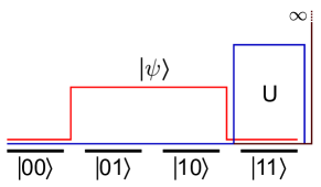
It is necessary for the initial wave packet to have some localization in space so that a distinct scattering event is visible, i.e., there is a point in time when the particle reaches the interaction region. As a side effect, the wave packet will have some momentum distribution because it no longer is a plane wave. As depicted in Fig. 2, we chose our initial wave packet to be $|\pi/2\rangle$ but restricted it to be non-zero only in the middle:

|\psi\rangle=\frac{1}{\sqrt{2}}\Big{(}|01\rangle+i|10\rangle\Big{)}.

(8)

We construct this wave packet on two sites with the following quantum circuit with all qubits initialized in the $|0\rangle$ state:

U_{\text{state prep}}=\begin{gathered}\Qcircuit@C=-1.5em@R=-4em@!{&\gate{X}&\multigate{1}{XX\Big{(}-\frac{3\pi}{2}\Big{)}}&\qw\\ &\qw&\ghost{XX\Big{(}-\frac{3\pi}{2}\Big{)}}&\qw}\end{gathered}.

(9)

The time evolution operator can be written as a combination of XX, YY, X, rotations and a controlled phase operation ( $R_{\phi}$ ):

\begin{matrix} U_{Tr} (ρ, θ) = \end{matrix}, w h e r e ρ = J δ t, θ = U δ t, a n d δ t = 12.5 . W e u s e s t a n d a r d n o t a t i o n s nielsen2000quantum f o r t h e g a t e s . T h e v e r y s l o w g r o w t h o f t h e o n e - s t e p e r r o r f o r l a r g e δ t ybook a l l o w s u s t o r e a c h t=75 w i t h o n l y s i x T r o t t e r s t e p s gustafson2019real . W e t h e n p e r f o r m a q u a n t u m F o u r i e r t r a n s f o r m (Q F T r) o n t h e s e t w o q u b i t s t o t a k e t h i s s t a t e i n t o m o m e n t u m s p a c e : (11)Equation 11eq.Equationeqs.Equations11UQFTr=\Qcircuit@C=-1em@R=-2em@!&\qw\gateRϕ(π/2)\gateH\qw. A f t e r a p p l y i n g t h e Q F T r, t h e q u b i t s t a t e s —10 ⟩ a n d —11 ⟩ c o r r e s p o n d t o t h e m o m e n t u m s t a t e s —k ⟩ a n d | - k ⟩ r e s p e c t i v e l y, w i t h k= π /2 . W e d e f i n e t h e p r o b a b i l i t i e s t o b e i n t h e —±k ⟩ s t a t e (12)Equation 12eq.Equationeqs.Equations12P±(t)≡|⟨±k|ψ(t)⟩|2, a n d t h e i r r e n o r m a l i z e d v e r s i o n s (13)Equation 13eq.Equationeqs.Equations13R±(t)≡P±(t)P+(t)+P-(t) w h i c h b y d e s i g n s a t i s f y (14)Equation 14eq.Equationeqs.Equations14R++R-=1. T h e r e a l - t i m e e v o l u t i o n p r o v i d e s t h e t i m e t^⋆ n e c e s s a r y t o r e a c h t h e s y m m e t r i c s i t u a t i o n w h e r e P_+(t^⋆)=P_- (t^⋆) . T h i s c o r r e s p o n d s t o t h e t i m e w h e r e a c l a s s i c a l p a r t i c l e w o u l d h i t t h e b a r r i e r . W e c a n t h e n c o m p a r e t^⋆ i n t h e c a s e w h e r e U = 0 a n d U = 0.03 a n d w e c a l l t h e s e t i m e s t^⋆_free a n d t^⋆_int. r e s p e c t i v e l y . I n o r d e r t o d e t e r m i n e t h e d i f f e r e n c e (15)Equation 15eq.Equationeqs.Equations15Δt⋆≡t⋆int.-t⋆free=ΔtW2 T h e r e l a t i o n t o t h e t i m e d e l a y Δt _W u s e d i n E q . (6) i s s u p p o r t e d b y n u m e r i c a l c a l c u l a t i o n s p r o v i d e d l a t e r . T h i s r e l a t i o n c a n a l s o b e j u s t i f i e d f r o m t h e t i m e - r e v e r s a l a r g u m e n t t h a t a f t e r t^⋆_int. o n l y ℎ𝑎𝑙𝑓 o f t h e p h a s e s h i f t, δ (k), h a s b u i l t u p w h i l e t h e o t h e r h a l f b u i l d s a f t e r t^⋆ . T h i s i s w h y h i s t o r i c a l l y, t h e t o t a l p h a s e s h i f t i s d e n o t e d 2 δ (k) . T h e t i m e t^⋆ i s d e t e r m i n e d b y t h e s y m m e t r i c c o n d i t i o n R_-(t^⋆)=R_+(t^⋆)=0.5 . T h i s r e q u i r e s s o m e c o n t i n u o u s i n t e r p o l a t i o n a m o n g t h e d i s c r e t e v a l u e s a t t h e T r o t t e r s t e p s . W e f i n d t h a t t h e s i g m o i d p a r a m e t r i z a t i o n (16)Equation 16eq.Equationeqs.Equations16R±(t)≃1/(1+exp(∓(t-t⋆w))), p r o v i d e s v e r y g o o d f i t s o f t h e n u m e r i c a l d a t a a n d s a t i s f i e s t h e s u m r u l e o f E q . (14) b e c a u s e o f i t s r e f l e c t i o n p r o p e r t y . T h i s a l s o i m p l i e s t h a t t h e t i m e r e v e r s a l w i t h r e s p e c t t o t^⋆ a m o u n t s t o t h e m o m e n t u m r e v e r s a l . T h e p a r a m e t e r w d e s c r i b e s t h e w i d t h o f t h e s i g m o i d . T h e d a t a f o r R_- o b t a i n e d f r o m b o t h q u a n t u m c o m p u t e r s a r e s h o w n i n F i g . LABEL:fig:wallscatter t o g e t h e r w i t h t h e s i g m o i d f i t s w h e r e t h e v a l u e s o f t^⋆_free a n d t^⋆_int. a r e i n d i c a t e d b y v e r t i c a l l i n e s c r o s s i n g t h e f i t s a t t h e 0.5 h o r i z o n t a l l i n e . T h i s p r o v i d e s t h e n u m e r i c a l v a l u e s o f Δt^⋆ g i v e n i n T a b l e LABEL:tab:tstar . F o r c o m p a r i s o n, w e g i v e t h e v a l u e s o b t a i n e d b y d o i n g s i g m o i d f i t s o f t h e c o n t i n u o u s - t i m e e v o l u t i o n (f i r s t c o l u m n) a n d t h e T r o t t e r s t e p s (s e c o n d c o l u m n) c a l c u l a t e d n u m e r i c a l l y a t t h e s a m e d i s c r e t e t i m e s a s t h e e x p e r i m e n t a l d a t a . T h e s y s t e m a t i c e r r o r s a r e e x p e c t e d t o b e l a r g e r t h a n t h e s t a t i s t i c a l e r r o r s a n d v e r y d i f f i c u l t t o e s t i m a t e . D e t a i l s o f t h e f i t s a r e g i v e n i n t h e S u p p l e m e n t a r y M a t e r i a l (S M) . W e s e e t h a t b o t h t h e I B M a n d t r a p p e d i o n e s t i m a t e s p r o v i d e l a r g e r a b s o l u t e v a l u e s o f Δt^* t h a n t h e t a r g e t v a l u e s . T h i s c a n b e i n p a r t e x p l a i n e d b y t h e f a c t t h a t t h e f i t s f o r t h e f r e e p r o c e s s t e n d t o l a g b e l o w t h e T r o t t e r s t e p s f o r t¿50 i n d i c a t i n g a l o s s o f c o h e r e n c e . M e a s u r e m e n t s f r o m t h e I B M Q B o g o t a m a c h i n e c o n t a i n b o t h t h e n o i s y d a t a w i t h j u s t r e a d o u t c o r r e c t i o n s a n d a m i t i g a t e d v e r s i o n o b t a i n e d u s i n g m e t h o d s d i s c u s s e d i n R e f . gustafson2019real a n d w h i c h a c c o u n t f o r s o m e s l i g h t l y n e g a t i v e o c c u p a t i o n s a t l o w t . T h e t r a p p e d i o n s i m u l a t i o n s i n c l u d e o n l y r e a d o u t c o r r e c t i o n s w i t h o u t n o i s e m i t i g a t i o n (s e e S M) . W e s e e t h a t t h e q u a n t u m m e c h a n i c s a p p r o x i m a t i o n a l l o w s u s t o p e r f o r m t h e Q F T r a n d g e t r e a s o n a b l e e s t i m a t e s o f Δt^*, (T a b l e LABEL:tab:tstar) . W e e x p e c t t o i m p r o v e t h e a c c u r a c y o f t h e s e e s t i m a t e s i n t h e n e a r f u t u r e . T h e e x t e n s i o n o f t h i s p r o c e d u r e f o r m o r e t h a n f o u r s i t e s r e q u i r e s a n a l l - t o - a l l c o n n e c t i v i t y a n d a C N O T d e p t h i n c r e a s i n g w i t h t h e n u m b e r o f s i t e s . I n c o n t r a s t, t h e f i e l d t h e o r y c a l c u l a t i o n d i s c u s s e d i n t h e n e x t s e c t i o n, a n d w h i c h i s o u r u l t i m a t e g o a l, r e q u i r e s m o r e q u b i t s b u t r e m a i n s l o c a l Lloyd1073 w i t h a c o n s t a n t C N O T d e p t h . Figure 4Figure 4fig.Figurefigs.Figures4Figure 43Exper

(S12)