Fast hyperspectral image denoising and inpainting
based on low-rank and sparse representations

Abstract

This paper introduces two very fast and competitive hyperspectral image (HSI) restoration algorithms: Fast Hyperspectral Denoising (FastHyDe), a denoising algorithm able to cope with Gaussian and Poissonian noise, and Fast Hyperspectral Inpainting (FastHyIn), an inpainting algorithm to restore HSIs where some observations from known pixels in some known bands are missing. FastHyDe and FastHyIn fully exploit extremely compact and sparse HSI representations linked with their low-rank and self-similarity characteristics. In a series of experiments with simulated and real data, the newly introduced FastHyDe and FastHyIn compete with state-of-the-art methods, with much lower computational complexity. A MATLAB demo of this work is available at www.lx.it.pt/~bioucas/code/Demo_FastHyDe_FastHyIn.rar for the sake of reproducibility.

I Introduction

Hyperspectral remote sensing images have been widely used in countless applications (e.g., earth observation, environmental protection and natural disaster monitoring), owing to their remarkably high spectral resolution (hundreds or thousands spectral channels), which enables precise material identification via spectroscopic analysis [1]. However, this potential is often compromised due to low quality of the hyperspectral images (HSIs), linked with various degradation mechanisms, such as electronic noise, Poissonian noise, quantization noise, stripe noise, and atmospheric effects.

As the number of spectral bands increases in the new-generation hyperspectral sensors, the spectral bandwidth decreases implying that, everything else kept constant, each spectral channel receives less photons, yielding higher levels of Poissonian noise. So Poissonian noise is becoming the main concern in real hyperspectral images [2, 3, 4]. If the mean values of the photon counts is larger than 4, then Poissonian noise can be converted into approximately additive Gaussian noise with nearly constant variance using variance-stabilizing transformations [5]. This opens a door to use available algorithms designed for additive Gaussian noise [6]. In this paper, we assume that the observation noise is either additive Gaussian or Poissonian. In the latter case, and prior to restore the noisy image, the Poissonian noise is converted into approximate additive Gaussian noise by applying a variance-stabilizing transformation.

Natural images are self-similar. This means that they contain many similar patches at different locations and scales. This characteristic has been recently exploited by the patch-based image restoration methods and holds the state-of-the-art in image denoising. Representative examples of this methodology in single-band images include the non-local means filter [7], the Gaussian mixture model (GMM) learned from the noisy image [8], and the collaborative filtering of groups of similar patches BM3D [9], LRCF [10], and EPLL [11]. Identical ideas have been pursued in multi-band image denoising: BM4D [12], VBM4D [13], and MSPCA-BM3D [14] use collaborative filtering in groups of 3D patches extracted from volumetric data, videos, multispectral data, respectively. DHOSVD [15] applies hard threshold filtering to the higher order SVD coefficients of similar patches.

In HSI denoising, besides the spatial information, the high correlation in spectral domain has also been widely investigated, as it implies that the spectral vectors live in low-dimensional manifolds or subspaces [1, 16], admitting, therefore, extremely compact and sparse representations on suitable frames. These characteristics have been exploited, namely, in low-rank matrix approximation [17, 18, 19, 20, 21], in the structured tensor TV-based regularization [22], and in the adaptive spectrum-weighted sparse Bayesian dictionary learning method (ABPFA) [23]. Sparse representations have also been exploited in many inverse problems in hyperspectral imaging, for example, classification (see more details in [24, 25, 26]).

Image inpainting is the process of image reconstruction from incomplete observation. For single-band images, spatial information from areas with complete observations is used to inpaint the incomplete observations, i.e., the missing pixels. Inpainting techniques mainly exploit spatial information of consistent geometric structure [27], texture with repetitive patterns [28], and combinations of both [29]. Structural inpainting focuses on the consistency of the geometric structure by enforcing a smoothness prior to preserve edges or isophotes. The consistency of structure may be enforced using partial differential equations [30], total variation [31, 22], and Markov random field image priors [32]. But enforcing consistent structure does not restore texture. This calls for textural inpainting, which tries to capture textures with a repetitive pattern and complete the missing region using its similar neighbourhood. Textural inpainting may not be able to keep consistency in the boundaries between image regions. Since most part of an image consist of structure and texture, the state-of-the-art inpainting methods attempt to combine structural and textural inpainting. For example, [29] decomposes the image into the sum of two functions with different basic characteristics, and then reconstruct each one of these functions separately with structure and texture inpainting algorithms. Exemplar-based image inpainting fills missing regions of an image by searching for similar patches in a neighboring region of the image, and copying the pixels from the most similar patch into the missing region [33, 7].

For multispectral and HSIs inpainting, coherence lying in temporal, spatial, or spectral domains is exploited. For example, the spatiotemporal relationships between a sequence of multitemporal images were studied in [34, 35] to reconstruct corrupted regions. Spectral coherence between a damaged band and other bands was exploited in [23]. In [36], both spatial and spectral coherence were achieved via a multichannel non-local total variation inpainting model.

From the above considerations, it may be concluded that denoising and inpainting approaches share a number of similar techniques to promote spatial-spectral coherence. In fact, from the formal point of view, the inpainting restoration problem may be interpreted as a denoising one with missing observations, whose locations are known [36].

I-A Contribution

Most of the published hyperspectral denoising and inpainting algorithms are time-consuming, namely due to the large sizes of HSIs and, often, due to the implementation of iterative estimation procedures both in the spatial and the spectral domains. In an effort to mitigate these shortcomings, this paper introduces a fast hyperspectral denoising (FastHyDe) approach and its fast hyperspectral inpainting (FastHyIn) extension.

FastHyDe and FastHyIn take full advantage of the HSIs’ low-rank structure and self-similarity referred to above: 1) the low-rank structure of HSI is fully exploited by representing the spectral vectors of the clean image in a pre-learned subspace; 2) we claim that the images of subspace coefficients are self-similar (see Claim 1) and can be denoised component by component using non-local patch-based single band denoisers. Groups of similar non-local patches admit sparse representations which underlies strong noise attenuation.

This work is an extension of the material published in [6]. The new material is the following: a) FastHyDe is herein introduced and characterized in more detail; b) a new algorithm, termed FastHyIn, to solve inpainting inverse problems is introduced; and c) exhaustive array of experiments and comparisons is carried out.

The paper is organized as follows. Section II introduces formally FastHyDe, a denoising approach based on low-rank and sparse representations. Its inpainting version, FastHyIn, is given in Section III. Section IV and V present experimental results including comparisons with the state of the art. Section VI concludes the paper.

II Formulation and proposed denoiser

Let ${\bf X}:=[{\bf x}_{1},\dots\bf x_{n}]\in\mathbb{R}^{n_{b}\times n}$ denote a HSI with $n$ spectral vectors (the columns of $\bf X$) of size $n_{b}$. The rows $\bf X$ contain $n_{b}$ spectral bands, which are images, corresponding to the scene reflectance in a given wavelength interval, with $n$ pixels organized in a grid in the spatial domain. In hyperspectral denoising problems under the additive noise assumption, the observation model may be written as

$$\mathbf{Y=X+N},$$ (1)

where $\mathbf{Y,N}\in\mathbb{R}^{n_{b}\times n}$ represent the observed HSI data and noise, respectively.

We assume that the spectral vectors ${\bf x}_{i}$, for $i=1,\dots,n$, live in a $k-$dimensional subspace ${\cal S}_{k}$, with $n_{b}\gg k$. This is a very good approximation in most real HSIs [1]. Therefore, we may write

$$\mathbf{X=EZ},$$ (2)

where the columns of $\mathbf{E}=[{\bf e}_{1},\dots,{\bf e}_{k}]\in\mathbb{R}^{n_{b}\times k}$ holds a basis for ${\cal S}_{k}$ and matrix $\mathbf{Z}\in\mathbb{R}^{k\times n}$ holds the representation coefficients of $\bf X$ with respect to (w.r.t.) $\bf E$. We assume, without loss of generality, that $\bf E$ is semi-unitary, that is ${\bf E}^{T}{\bf E}={\bf I}_{k}$ with ${\bf I}_{k}$ representing the identity matrix of dimension $k$. Matrix $\bf E$ may be learned from the data using, e.g., the HySime algorithm [16] or singular value decomposition (SVD) of $\bf Y$ in the case the noise is independent and identically distributed (i.i.d.). We will herein term the images associated with the rows of $\bf Z$ as eigen-images.

Images of the real world are self-similar, that is, they contain many similar patches at different locations and scales. The exploitation of self-similarity, as a form of prior knowledge/regularization, underlies the state-of-the-art in imaging inverse problems. HSI bands, being images of the real world, are self-similar. Furthermore, since each band corresponds to the reflectance, in a given wavelength interval, of the same surface, the spatial structure of the self-similarity is identical across all bands. This has a fundamental relevance for the proposed approach stated in the following claim.

Claim 1

The eigen-images associated to the rows of ${\bf Z}$ are self-similar.

Justification: Since $\bf E$ is semi-unitary, then ${\bf Z}={\bf E}^{T}{\bf X}$, and therefore the eigen-images are linear combinations of the the bands of $\bf X$. Given that the bands of $\bf X$ are self-similar and have the same self-similarity spatial structure, then the eigen-images are self-similar. $\square$

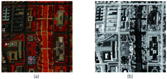
Figure 1: False color composites of the Washington DC Mall subscene (a) and its 1st band of eigen-images (b).

Fig. 1 shows in the left hand side a false color image of the a Washington DC Mall subscene and in the right hand side the eigen-image corresponding to the first column of $\bf E$. Clearly, the eigen-image preserves the self-similar structure of the corresponding color image.

This paper explores two main characteristics of hyperspectral data: 1) HSIs live in low dimensional subspaces, which opens the door to remove the bulk of the noise using projection-based methods [1]; 2) the eigen-images are self-similar and, therefore, they may be denoised with non-local patch-based methods such as BM3D [9] and LRCF [10].

Below we start by considering that the noise is additive Gaussian and i.i.d. Later, we consider additive Gaussian non-i.i.d and Poissonian noise.

II-A Additive Gaussian i.i.d. noise

In the first case, we consider that the noise is additive zero-mean Gaussian and i.i.d. over all components of $\bf N$. Assuming that the subspace $\mathbf{E}$ has been learned from the observed data $\bf Y$, the eigen-images denoising problem is formulated as

$$\begin{split}\widehat{\mathbf{Z}}&\in\arg\min_{\mathbf{Z}}\frac{1}{2}\|\mathbf{EZ-Y}\|_{F}^{2}+\lambda\phi(\mathbf{Z})\\ &=\arg\min_{\mathbf{Z}}\frac{1}{2}\|\mathbf{Z-E}^{T}{\bf Y}\|_{F}^{2}+\lambda\phi(\mathbf{Z}),\end{split}$$ (3)

where $\|{\bf X}\|_{F}=\sqrt{\text{trace}({\bf XX}^{T})}$ is the Frobenius norm of $\bf X$. The optimization problems in (3) are equivalent since ${\bf E}$ is semi-unitary and ${\bf E}^{T}{\bf E}={\bf I}$. The first term on the right-hand of side (3) represents the data fidelity and accounts for the zero-mean Gaussian i.i.d noise, while the second term is a regularizer expressing prior information tailored to self-similar images.

We assume that the function $\phi$ is decoupled w.r.t. the eigen-images, that is

$$\phi(\mathbf{Z})=\sum_{i=1}^{k}\phi_{i}(\mathbf{Z}^{i})$$ (4)

where $\mathbf{Z}^{i}$ is the $i$th eigen-image, i.e., the $i$th row of $\bf Z$. An informal justification for the decoupling is that the components of $\bf Z$ tend to be decorrelated. Although decorrelation does not imply statistical independence, it is a necessary condition for it. In practice, this assumption leads to excellent results as shown in Section IV. Another relevant observation is that the noise associated to the term ${\bf E}^{T}\bf Y$ is still i.i.d. with the same variance as the original components of $\bf N$. In fact,

$${\bf E}^{T}{\bf Y}={\bf Z}+{\bf E}^{T}{\bf N},$$

and therefore the columns of the noise term ${\bf E}^{T}{\bf N}$ are independent and, given $\bf n$, a generic column of $\bf N$, we have

$$\mathbb{E}[{\bf E}^{T}{\bf n}{\bf n}^{T}{\bf E}]={\bf E}^{T}\mathbb{E}[{\bf n}{\bf n}^{T}]{\bf E}=\sigma^{2}{\bf E}^{T}{\bf E}=\sigma^{2}{\bf I}_{k},$$

where $\sigma^{2}$ is the variance of a generic element of $\bf N$. Therefore, ${\bf E}^{T}{\bf n}\sim{\cal N}({{\bf 0},\sigma^{2}{\bf I}_{k}})$, this is, ${\bf E}^{T}{\bf n}$ is zero-mean Gaussian with covariance $\sigma^{2}{\bf I}_{k}$.

Under the hypothesis (4), the solution of (3) is decoupled w.r.t. ${\bf Z}^{i}$ and may be written as

$$\widehat{\mathbf{Z}}=\psi_{\lambda\phi}(\mathbf{E}^{T}{\bf Y})=\left[\begin{array}[]{c}\psi_{{\lambda\phi}_{1}}(\mathbf{e}_{1}^{T}\mathbf{Y})\\ \vdots\\ \psi_{{\lambda\phi}_{k}}(\mathbf{e}_{k}^{T}\mathbf{Y})\end{array}\right],$$ (5)

where

$$\psi_{{\lambda\phi}_{i}}({\bf y})=\arg\min_{\bf w}\frac{1}{2}\|{\bf y-w}\|^{2}_{F}+\lambda\phi_{i}({\bf w})$$ (6)

is the so-called denoising operator, or Moreau proximity operator of $\phi_{i}$ [37]. In this paper, we resort to the plug-and-play (PnP) prior framework [38] to address the denoising problem (6). The central idea in PnP is, instead of investing efforts in tailoring regularizers promoting self-similar images and then computing its proximity operators, to use directly a state-of-the-art denoiser conceived to enforce self-similarity, such as BM3D [9], LRCF [10], and GMM [8]. A pertinent question in the PnP approach is that, given a denoiser, weather there exists a convex regularizer of which the denoiser is the proximity operator. The answer for BM3D, LRCF, and GMM is negative [39, 40], as it is for most state-of-the-art denoisers. This fact should not prevent us, however, to use such denoisers as they are effective in promoting self-similar images. In this work, we selected BM3D, as it is the state-of-the-art and a very fast implementation thereof is publicly available.

The proposed algorithm for HSI denoising, termed Fast Hyperspectral denoising (FastHyDe), is summarized in Algorithm 1. Step 2 learns $\bf E$, e.g., using HySime, step 3 and step 4 compute and denoise the eigen-images, respectively, and step 5 reconstructs the estimate of the original data.

Algorithm 1 FastHyDe for i.i.d. noise

1:Input Noisy HSI data $\mathbf{Y}$ and the noise variance $\sigma^{2}$.

2:Learn the subspace $\mathbf{E}$ from observations $\bf Y$ and compute the noisy eigen-images $\mathbf{E}^{T}\mathbf{Y}$.

3:Compute ${\widehat{\bf Z}}$ by denoising the eigen-images one by one, using a state-of-the-art denoising algorithm.

4:Compute $\widehat{\mathbf{X}}=\mathbf{E\widehat{Z}}$, an estimate of the clean HSI.

Note that the dimension of subspace ${\bf E}$ can be estimated by HySime or by any other subspace identification method. We provide evidence in the experiments that, as far as the subspace dimension is not underestimated, FastHyDe is extremely robust to errors in estimation of the subspace dimension.

II-B Additive Gaussian non-i.i.d. noise

Consider that in the observation model (1), $\mathbf{N}$ is zero-mean, additive, Gaussian, pixelwise independent with spectral covariance $\mathbf{C}_{\lambda}=E[{\bf n}_{i}{\bf n}^{T}_{i}]$, where ${\bf n}_{i}$ is a generic column of $\bf N$. Notice that in the i.i.d. case $\mathbf{C}_{\lambda}=\sigma^{2}{\bf I}$, which is not the case in the non-i.i.d. scenario. We assume that ${\bf C}_{\lambda}$ is positive definite and therefore non-singular. In order to reconvert the non-i.i.d. scenario into the i.i.d. one, the observed data is whitened as

$$\mathbf{\widetilde{Y}}:=\sqrt{\mathbf{C}_{\lambda}^{-1}}\mathbf{Y},$$ (7)

where $\sqrt{\mathbf{C}_{\lambda}^{-1}}$ is a matrix denoting the square root of $\mathbf{C}_{\lambda}^{-1}$ and $\sqrt{\mathbf{C}_{\lambda}}$ denotes its inverse. Then the observation model of $\mathbf{\widetilde{Y}}$ becomes

$$\mathbf{\widetilde{Y}}=\sqrt{\mathbf{C}_{\lambda}^{-1}}\mathbf{X}+\sqrt{\mathbf{C}_{\lambda}^{-1}}\mathbf{N}=\mathbf{\widetilde{X}}+\mathbf{\widetilde{N}}.$$ (8)

The noise covariance matrix of $\widetilde{\bf n}_{i}$, a generic column of $\widetilde{\bf N}_{i}$, is

$$\mathbf{\widetilde{C}}_{\lambda}=E[\widetilde{\bf n}_{i}\widetilde{\bf n}^{T}_{i}]=\mathbf{I}.$$ (9)

Since the noise in (9) is i.i.d., we may again formulate the denoising problem as

$$\mathbf{\widehat{\widetilde{Z}}}=\arg\min_{\mathbf{\widetilde{Z}}}\frac{1}{2}\Big{\|}\mathbf{\widetilde{Z}-\widetilde{E}}^{T}{\bf\widetilde{Y}}\Big{\|}_{F}^{2}+\lambda\phi(\mathbf{\widetilde{Z}}),$$ (10)

where $\widetilde{\mathbf{E}}$ holds an orthonormal basis learned from $\widetilde{\mathbf{Y}}$. The solution of (10) can be found following the same steps described in Algorithm 1. The clean data of $\widetilde{\mathbf{Y}}$ is estimated as

$$\widehat{\widetilde{\mathbf{X}}}=\widetilde{\mathbf{E}}\widehat{\widetilde{\mathbf{Z}}},$$ (11)

followed by recovering the original clean data $\mathbf{X}$ from $\widetilde{\mathbf{X}}$

$$\widehat{\mathbf{X}}=\sqrt{\mathbf{C}_{\lambda}}\widehat{\widetilde{\mathbf{X}}}.$$ (12)

III Fast Inpainting

The clean image ${\bf X}\in{\mathbb{R}}^{n_{b}\times n}$ may be vectorized as ${\bf x}={\rm vec}({\bf X})\in\mathbb{R}^{t}$, $(t=n_{b}\times n)$, where $\rm vec$ stacks the columns of ${\bf X}$. In hyperspectral inpainting problems under the additive noise, the observation model may then be written as

$$\mathbf{y}=\mathbf{M}\mathbf{x}+\mathbf{n}$$ (13)

where $\mathbf{y}\in\mathbb{R}^{q}$, with $q\leq t$, and $\mathbf{n}\in\mathbb{R}^{q}$ represents the observed incomplete data and noise, respectively. The matrix $\mathbf{M}\in\mathbb{R}^{q\times t}$ is a mask that selects a subset of the components of $\bf x$. It is thus a binary matrix corresponding to a subset of rows of an identity matrix, therefore having only one 1 per row. We assume that $\mathbf{M}$ is user-provided.

Below we start by considering Gaussian i.i.d. noise. Later, we consider Gaussian non-i.i.d and Poissonian noise.

III-A Additive Gaussian i.i.d. noise

By still assuming that the spectral vectors belong to subspace spanned by the columns of $\bf E$, and thus , $\mathbf{X=EZ}$, we have

$$\mathbf{x}:=\rm vec({\bf EZ})=(\mathbf{I}\otimes\mathbf{E})\mathbf{z},$$ (14)

where $\otimes$ represents Kronecker product and $\mathbf{z}:=\text{vec}(\mathbf{Z})$. The inpainting problem is formulated as

$$\min_{\mathbf{z}}\frac{1}{2}\|\mathbf{M}(\mathbf{I}\otimes\mathbf{E})\mathbf{z}-\mathbf{y}\|^{2}+\lambda\phi(\mathbf{z}).$$ (15)

Instead of solving (15), which involves a non-diagonal operator, thus, calling for iterative solvers, we propose a suboptimal solution that is very fast and effective. Let ${\bf M}_{i}$ be the submatrix of $\bf M$ acting on the pixel $i$, and

$${\bf y}_{o,i}=\mathbf{M}_{i}{{\bf x}}_{i}+{{\bf n}}_{o,i}\in{\mathbb{R}}^{n_{i}},$$ (16)

be the observed vector at the same pixel, where $n_{i}\leq n_{b}$ denotes the number of observed components at that pixel, and the vector ${{\bf n}}_{o,i}\in{\mathbb{R}}^{n_{i}}$ denotes the corresponding noise components. Since ${\bf x}_{i}={\bf Ez}_{i}$, we may write

$${\bf y}_{o,i}=\mathbf{M}_{i}{\bf Ez}_{i}+{{\bf n}}_{o,i}.$$ (17)

The least squares estimator of coefficients of subspace representation ${{\bf z}}_{i}$ is given by

$$\widehat{{{\bf z}}}_{i}=(\mathbf{E}^{T}\mathbf{M}_{i}^{T}\mathbf{M}_{i}\mathbf{E})^{-1}\mathbf{E}^{T}\mathbf{M}_{i}^{T}{{\bf y}}_{o,i},$$ (18)

where it is assumed that the matrix $\mathbf{E}^{T}\mathbf{M}_{i}^{T}\mathbf{M}_{i}\mathbf{E}$ is non-singular and thus that $n_{i}\geq k$. That is, the number of observed components is larger or equal than the dimension of the signal subspace.

After recovering the unobserved component at each pixel by computing $\widehat{{\bf y}}_{i}=\mathbf{E}\widehat{{{\bf z}}}_{i}$, for $i=1,\dots,n$, we solve the denoising problem

$$\min_{\mathbf{z}}\frac{1}{2}\|(\mathbf{I}\otimes\mathbf{E})\mathbf{z}-\widehat{\mathbf{y}}\|^{2}+\lambda\phi(\mathbf{z}),$$ (19)

where $\widehat{\mathbf{y}}:=\text{vec}\,[\widehat{{\bf y}}_{1},\dots,\widehat{{\bf y}}_{n}]$. Problem (19) is equivalent to

$$\min_{\mathbf{Z}}\frac{1}{2}\|\mathbf{EZ}-\widehat{\mathbf{Y}}\|_{F}^{2}+\lambda\phi(\mathbf{Z}),$$ (20)

Optimization (20) is similar to (3) and, thus, we use FastHyDe to solve it.

At this point, we would like to remark that the pixels completely observed, that is $n_{i}=n_{b}$, are not affect by the computation of $\widehat{\bf z}_{i}$ given (18). In fact, when $n_{i}=n_{b}$, ${\bf M}_{i}$ is a diagonal matrix and we have $\widehat{\bf z}_{i}={\bf E}^{T}{\bf y}_{i}$, which is exactly the vector used in the the second equation in (3). Therefore, the computation (18) shall be applied just to the set of incomplete observed pixels.

The proposed approach for HSI inpainting, termed Fast Hyperspectral inpainting (FastHyIn), is summarized in Algorithm 2. As an extension of FastHyDe, FastHyIn turns into FastHyDe, when the inpainting mask is $\mathbf{M}=\mathbf{I}$.

Algorithm 2 FastHyIn for i.i.d. noise

1:Input the noisy and incomplete HSI data $\mathbf{y}$ and the inpainting mask $\mathbf{M}$

2:Learn the subspace $\mathbf{E}$ from completely observed pixels.

3:Compute the eigen-images $\hat{{\bf z}}_{i}$ according to (18), only for incompletely observed pixels.

4:Compute ${\widehat{\bf Z}}$ by denoising the eigen-images one by one, using a state-of-the-art denoising algorithm.

5:Compute $\widehat{\mathbf{X}}=\mathbf{E\widehat{Z}}$, an estimate of the clean HSI.

III-B Additive Gaussian non-i.i.d. noise

We may treat the non-i.i.d noise as the maximum likelihood (ML) estimation of ${\bf z}_{i}$ in (17) under zero-mean Gaussian noise with correlation ${\bf C}_{\lambda,i}={\bf M}_{i}{\bf C}_{\lambda}{\bf M}_{i}^{T}$. The solution is

$$\widehat{{{\bf z}}}_{i}=(\mathbf{E}^{T}\mathbf{M}_{i}^{T}{\bf C}_{\lambda,i}^{-1}\mathbf{M}_{i}\mathbf{E})^{-1}\mathbf{E}^{T}\mathbf{M}_{i}^{T}{\bf C}_{\lambda,i}^{-1}{{\bf y}}_{o,i}.$$ (21)

As in the i.i.d case, the coefficients (21) need to be computed just for the incompletely observed pixels. Algorithm 3 shows FastHyIn algorithm for non-i.i.d noise.

Algorithm 3 FastHyIn for non-i.i.d. noise

1:Input the noisy and incomplete HSI data $\mathbf{y}$ and the inpainting mask $\mathbf{M}$.

2:Learn the subspace $\mathbf{E}$ from completely observed pixels.

3:Compute $\widehat{{\bf z}}_{i}$ according to (21), only for incompletely observed pixels, and replace ${\bf y}_{o,i}$ with $\widehat{\bf y}_{i}={\bf E}\widehat{{\bf z}}_{i}$.

4:Whiten the observations using (7).

5:Recompute $\widetilde{\bf E}$, a basis for the subspace spanning the whitened data $\widetilde{\bf Y}$.

6:Compute ${\widehat{\bf Z}}$ by denoising the eigen-images one by one, using a state-of-the-art denoising algorithm.

7:Compute $\widehat{\mathbf{X}}=\sqrt{\bf C}_{\lambda}\widetilde{\mathbf{E}}\widehat{\bf Z}$, an estimate of the clean HSI.

Note that Algorithm 3 is applied to general Gaussian non-i.i.d. cases where noise is pixelwise independent but, possibly, bandwise dependent, meaning covariance matrix $\mathbf{C}_{\lambda}$ can be non-diagonal. Now let us consider a simpler non-i.i.d. case where noise is both pixelwise and bandwise independent, meaning covariance matrix $\mathbf{C}_{\lambda}$ is diagonal. In this case, Algorithm 3 can be simplified as follows: instead of implementing steps 1-4, we whiten the incomplete observed pixel ${\bf y}_{o,i}$, that is, we compute

$$\tilde{{\bf y}}_{o,i}:=\sqrt{\mathbf{C}_{\lambda,i}^{-1}}{\bf y}_{o,i},$$ (22)

where ${\bf C}_{\lambda,i}={\bf M}_{i}{\bf C}_{\lambda}{\bf M}_{i}^{T}$. The complete observed pixel can be also whiten using (22) with ${\bf M}_{i}={\bf I}$. After whitening data, we obtain $\tilde{{\bf y}}=[\tilde{{\bf y}}_{o,1}^{T},\tilde{{\bf y}}_{o,2}^{T},\dots,\tilde{{\bf y}}_{o,n}^{T}]^{T}$, whose noise is i.i.d. We may again formulate the inpainting problem w.r.t $\tilde{{\bf y}}$ with i.i.d. noise as in (15).

IV Evaluation with simulated data

IV-A Denoising experiments

Two semi-synthetic observed hyperspectral datasets were simulated using additive Gaussian noise or Poissonian noise. The clean images were obtained form the Pavia Centre subscene (of size $[200\times 200]({\rm pixels})\times 103({\rm bands})$) and the Washington DC Mall subscene (of size $[256\times 256]({\rm pixels})\times 191({\rm bands})$).

In order to simulate the clean images, 23 very low signal-to-noise bands, due to the water vapor absorption, were removed. The remaining spectral vectors, in the two data sets, were projected on a signal subspace learned via SVD. The dimensions of the signal subspace for the Washington DC Mall subscene and the Pavia Centre subscene were set to 8. The projection preserves the bulk of the signal energy and largely reduces the noise. The projected HSIs of high quality are considered clean images in this section. Before adding simulated noise, each band of clean HSIs are normalized to [0, 1] as in [17]. We remark that the normalization is a linear and invertible operation that does not modify the signal-to-noise-ratio (SNR) of the corresponding band and that may be reverted after the denoising. The band 70 of the clean images of the Washington DC Mall subscene and of the Pavia Centre subscene is shown in the top left hand side of Figs. 3 and 4, respectively.

Three kinds of additive noises are considered:

Case 1

(Gaussian i.i.d. noise): ${\bf n}_{i}\sim{\cal N}({\bf 0},{\bf\sigma}^{2}{\bf I})$ with $\sigma\in\{0.02,0.04,0.06,0.08,0.10\}$.

Case 2

(Gaussian non-i.i.d. noise): ${\bf n}_{i}\sim{\cal N}({\bf 0},{\bf D}^{2})$ where $\bf D$ is a diagonal matrix with diagonal elements sampled from a Uniform distribution $U(0,1)$.

Case 3

(Poissonian noise): ${\bf Y}\sim{\cal P}(\alpha{\bf X})$, where ${\cal P}(\bf A)$ stands for a matrix of size$({\bf A})$ of independent Poisson random variables whose parameters are given by the corresponding element of ${\bf A}:=[a_{ij}]$. The parameter $\alpha$ is such that SNR$\,:=\alpha(\sum_{i,j}a_{ij}^{2})/(\sum_{ij}a_{ij})$ was set 15 dB.

The proposed FastHyDe is compared with BM3D [9], applied band by band, BM4D [12], ‘PCA+BM4D’ [41], and NAILRMA [17]. Since all the compared methods assume i.i.d. noise, the observed data in Case 2 and Case 3 are transformed in order to to have additive i.i.d. noise before the denoisers are applied. In case 2, we applied the transformation (7). In case 3, we applied the Anscombe transform $\mathbf{\widetilde{Y}}:=2\sqrt{\mathbf{Y}+\frac{3}{8}}$, which converts Poissonian noise into approximately additive noise [42].

We now discuss the parameter setting of the various algorithms. The parameters of FastHyDe and FastHyIn are the noise covariance matrix ${\bf C}_{\lambda}$ and the signal subspace, which are both computed by HySime [16]. BM3D and BM4D require the value of standard deviation of the noise as input parameter, which is estimated by HySime [16] as well. The remaining BM3D and BM4D parameters, namely the patch size $N1$, the sliding step $Nstep$, and the size of the search neighborhood $Ns$, are set to the default values stated in [9, 12]: $N1$=4, $Nstep$=3 $Ns$=11, for BM3D and, $N1$=8, $Nstep$=3, and $Ns$=39, for BM4D. The subspace dimension of two datasets input to FastHyDe and FastHyIn was set to 10, instead of 8, the true value, to provide evidence of the robustness of FastHyDe and FastHyIn with respect to subspace overestimation. The subspace dimension input to ‘PCA+BM4D’ was set to 8. For NAILRMA, the block size was set to 20 and step size to 8. These values were hand tuned to get optimal performance.

For quantitative assessment, the peak signal-to-noise (PSNR) index and the structural similarity (SSIM) index of each band are calculated. The corresponding mean PSNRs (MPSNR) and mean SSIMs (MSSIM) in Washington DC Mall data and in Pavia Centre are reported in Tabs. I and II, respectively. Dealing with different kinds of noises, FastHyDe yields uniformly the best performance with gains increasing as the noise increases, as it may be concluded from those results. High quality spectral signature is of critical importance to material identification. The quality of reconstructed spectra from different denoising methods may also be inferred from Figs. 3, 4, 5 and 6.

BM3D suits very well the eigen-images, which are self-similar. In addition, the fact that denoising is applied only to the eigen-images, which are much less than the number of bands, significantly reduces the FastHyDe complexity (see Tabs. III and IV), relative to the competitors. The algorithms were implemented using MATLAB R2010 on a desktop PC equipped with eight Intel Core i7-4970 CPU (at 3.60 GHz) and 16 GB of RAM memory.

FastHyDe robustness to subspace overestimation is illustrated in Fig 2. Take as example the noisy image of Washington DC Mall data generated in case 1 with $\sigma=0.10$ (Gaussian i.i.d. noise). The curve in red represents the energy of the original data $\bf X$ along the eigenvalue directions, that is, the values of $\|{\bf e}_{i}^{T}{\bf X}\|_{2}^{2}/n$, ordered by non-increasing magnitude. The straight line in green represents the noise variance. The curve in blue represents the PSNR yielded by FastHyDe for different values of the subspace dimension. It is clear that the PSNR is practically constant provided that the subspace dimension in not underestimated. That is to say that FastHyDe is extremely robust to the subspace dimension overestimation.

Figure 2: Power of signal and of noise and FastHyDe PSNR as a function of the dimension of the subspace estimation (the true subspace dimension is 8).

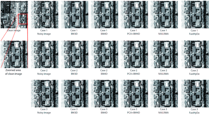
Figure 3: Denoising result for band 70 of DC Mall data with different kinds of noise. Case 1: Gaussian i.i.d. noise. Case 2: Gaussian non-i.i.d. Case 3: Poissonian noise

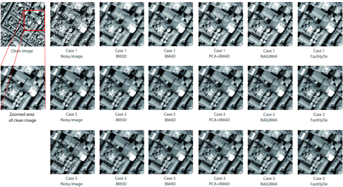
Figure 4: Denoising result for band 70 of Pavia Centre data with different kinds of noise. Case 1: Gaussian i.i.d. noise. Case 2: Gaussian non-i.i.d. Case 3: Poissonian noise.

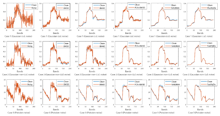
Figure 5: Denoised spectral signatures of Washington DC Mall data with different kinds of noise.

Figure 6: Denoised spectral signatures of Pavia Centre data with different kinds of noise.

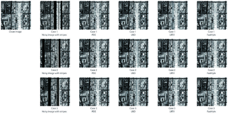
Figure 7: Destriping band 60 of Washington DC Mall with different kinds of noise. Case 1: Gaussian i.i.d. noise. Case 2: Gaussian non-i.i.d. Case 3: Poissonian noise.

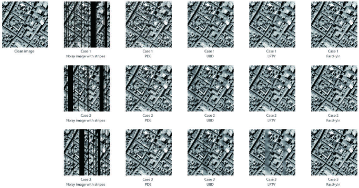
Figure 8: Destriping band 60 of Pavia Centre with different kinds of noise. Case 1: Gaussian i.i.d. noise. Case 2: Gaussian non-i.i.d. Case 3: Poissonian noise.

TABLE I: Quantitative assessment of different denoising algorithms applied to Washington DC Mall.

	$\sigma$	Index	Noisy Image	BM3D	BM4D	PCA+BM4D	NAILRMA	FastHyDe
Case 1	0.02	MPSNR(dB)	33.98	36.25	44.39	46.90	48.37	49.70
		MSSIM	0.9370	0.9663	0.9945	0.9960	0.9974	0.9981
	0.04	MPSNR(dB)	27.96	31.97	39.70	40.85	43.16	44.78
		MSSIM	0.8098	0.9166	0.9840	0.9845	0.9920	0.9945
	0.06	MPSNR(dB)	24.44	29.77	36.22	37.34	40.24	42.00
		MSSIM	0.6827	0.8677	0.9651	0.9666	0.9849	0.9902
	0.08	MPSNR(dB)	21.94	28.33	35.03	34.79	38.22	40.11
		MSSIM	0.5728	0.8253	0.9536	0.9435	0.9769	0.9854
	0.10	MPSNR(dB)	20.00	27.29	33.48	32.78	36.67	38.57
		MSSIM	0.4821	0.7848	0.9346	0.9169	0.9686	0.9801
Case 2		MPSNR(dB)	28.63	33.00	34.20	44.89	47.43	51.75
		MSSIM	0.7463	0.8942	0.9295	0.9893	0.9971	0.9987
Case 3		MPSNR(dB)	26.98	31.29	38.82	39.56	41.75	43.21
		MSSIM	0.7993	0.9118	0.9814	0.9804	0.9888	0.9919

TABLE II: Quantitative assessment of different denoising algorithms applied to Pavia Centre data.

	$\sigma$	Index	Noisy Image	BM3D	BM4D	PCA+BM4D	NAILRMA	FastHyDe
Case 1	0.02	MPSNR(dB)	33.98	36.67	44.58	43.09	46.66	47.09
		MSSIM	0.9328	0.9663	0.9939	0.9903	0.9959	0.9965
	0.04	MPSNR(dB)	27.96	32.68	39.98	37.03	41.71	42.58
		MSSIM	0.7950	0.9212	0.9832	0.9632	0.9874	0.9908
	0.06	MPSNR(dB)	24.44	30.56	37.39	33.45	38.87	40.03
		MSSIM	0.6550	0.8770	0.9701	0.9227	0.9770	0.9840
	0.08	MPSNR(dB)	21.94	29.11	35.55	30.93	36.80	38.32
		MSSIM	0.5362	0.8350	0.9556	0.8753	0.9646	0.9769
	0.10	MPSNR(dB)	20.00	28.06	34.11	29.00	35.31	36.99
		MSSIM	0.4417	0.7966	0.9393	0.8251	0.9541	0.9700
Case 2		MPSNR(dB)	29.77	34.29	35.05	39.70	46.94	49.26
		MSSIM	0.7445	0.9054	0.9225	0.9640	0.9970	0.9979
Case 3		MPSNR(dB)	26.97	32.18	39.46	35.95	40.53	41.59
		MSSIM	0.7595	0.9109	0.9817	0.9522	0.9848	0.9890

TABLE III: Computational time (seconds) of different denoising algorithms applied to Washington DC Mall data.

	$\sigma$	BM3D	BM4D	PCA+	NAILRMA	FastHyDe
				BM4D
Case 1	0.02	196	9679	9853	347	15
	0.04	208	9883	9588	236	14
	0.06	223	9698	8485	171	15
	0.08	205	8771	8405	149	14
	0.10	206	8865	8660	133	13
Case 2		198	8867	8481	27	16
Case 3		183	8899	8537	39	28

TABLE IV: Computational time (seconds) of different denoising algorithms applied to Pavia Centre data.

	$\sigma$	BM3D	BM4D	PCA+	NAILRMA	FastHyDe
				BM4D
Case 1	0.02	56	2118	1824	112	11
	0.04	56	2045	1773	72	9
	0.06	57	1995	1764	56	9
	0.08	59	2000	1753	51	9
	0.10	60	2004	1727	46	10
Case 2		48	1792	1607	9	7
Case 3		48	2189	1626	10	9

IV-B Inpainting experiments

This section evaluates the performance of FastHyIn by comparing it with three inpainting methods: the partial differential equations discretization (PDE) adapted to 3D data [43, 30], the unmixing based denoising (UBD) [44], and the total variation (TV)-regularized low-rank matrix factorization (LRTV) [19]. PDE method fills in selected regions with information surrounding them. UBD reconstructs damaged pixel using spectral unmixing results. LRTV models stripes as sparse noise, exploits spectral low-rank property via nuclear norm, and promotes spatial piecewise smoothness via TV regularization. In our experiments, spectral unmixing in UBD method is implemented as follows: The number of endmembers, their spectral signatures, and their abundances at each pixel are estimated by HySime [16], vertex component analysis [45] and non-negative constrained least squares, respectively.

The noisy images generated in case 1 with $\sigma=0.10$ (Gaussian i.i.d. noise), case 2 (Gaussian non-i.i.d) and case 3 (Poissonian noise) (see more details in Section IV-A) are used again to simulate corrupted images with stripes. Stripes are simulated for four bands (60th to 63rd bands) as shown in second columns in Figs. 7 and 8. The location of missing values is known beforehand and is an input variable in PDE, LRTV, and FastHyIn.

Destriping results are shown in Figs. 7 and 8. Visually, for Washington DC Mall data, almost all the methods are able to inpaint the dead lines, except LRTV in Case 1. For Pavia Centre data and in case 3, UBD and LRTV methods do not remove the stripes completely, as shown in Fig.8.

We remark that it is reasonable that output images of PDE are still noisy, because this method functions only as an inpainter and not as a denoiser. In contrast with this scenario, UBD, LRTV and FastHyIn remove noise largely while inpainting. Note that UBD reconstructs a clean image with estimated endmembers and abundances, meaning that its performance strongly depends on the results of spectral unmixing. Spectral unmixing is still a challenging problem in the realm of hyperspectral image processing [1, 46, 47]. For applying LRTV, the main challenge is to choose suitable regularization parameters. We have hand tuned them to get optimal performance in these experiments. We set rank $r$ = 8 (true value), the TV regularization parameter $\tau=0.015$ for all images, the sparsity regularization parameter $\lambda=70/{\sqrt{n}}$ for Pavia Centre data, and $\lambda=100/{\sqrt{n}}$ for Washington DC Mall data. FastHyIn is user-friendly. Similarly to FastHyDe, it involves only the noise covariance matrix ${\bf C}_{\lambda}$ and the signal subspace, which are both compute by HySime [16]. To provide evidence of FastHyIn robustness to overestimation of the subspace dimension, we set the subspace dimension $k=10$ instead of $k=8$, the true value. Regarding removal of noise, we can see from Tabs. V and VI that FastHyIn yields uniformly the best results in terms of MPSNR and MSSIM.

TABLE V: Quantitative assessment of different inpainting algorithms applied to Washington DC Mall.

	Index	Noisy Image	PDE	UBD	LRTV	FastHyIn
Case 1	MPSNR	19.90	20.01	34.52	35.53	38.58
	MSSIM	0.4794	0.4831	0.9575	0.9535	0.9802
	Time	-	26	23	210	12
Case 2	MPSNR	28.43	28.63	35.46	41.88	51.63
	MSSIM	0.7414	0.7466	0.9648	0.9853	0.9987
	Time	-	35	23	210	13
Case 3	MPSNR	26.80	26.99	37.18	40.78	43.21
	MSSIM	0.7952	0.7996	0.9780	0.9831	0.9919
	Time	-	26	26	179	24

TABLE VI: Quantitative assessment of different inpainting algorithms applied to Pavia Centre data.

	Index	Noisy Image	PDE	UBD	LRTV	FastHyIn
Case 1	MPSNR	19.79	20.04	33.68	33.38	36.95
	MSSIM	0.4335	0.4441	0.9335	0.9103	0.9698
	Time	-	1	12	49	6
Case 2	MPSNR	28.93	29.40	35.73	39.62	48.60
	MSSIM	0.7308	0.7454	0.9629	0.9565	0.9975
	Time	-	1	11	49	6
Case 3	MPSNR	26.51	27.00	35.90	38.58	41.54
	MSSIM	0.7453	0.7604	0.9647	0.9649	0.9889
	Time	-	1	13	49	7

V Evaluation with Real data

V-A Denoising experiments

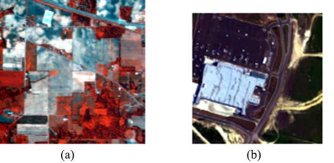
Figure 9: False color composite of Indian Pine data (a) and Urban subscene (b).

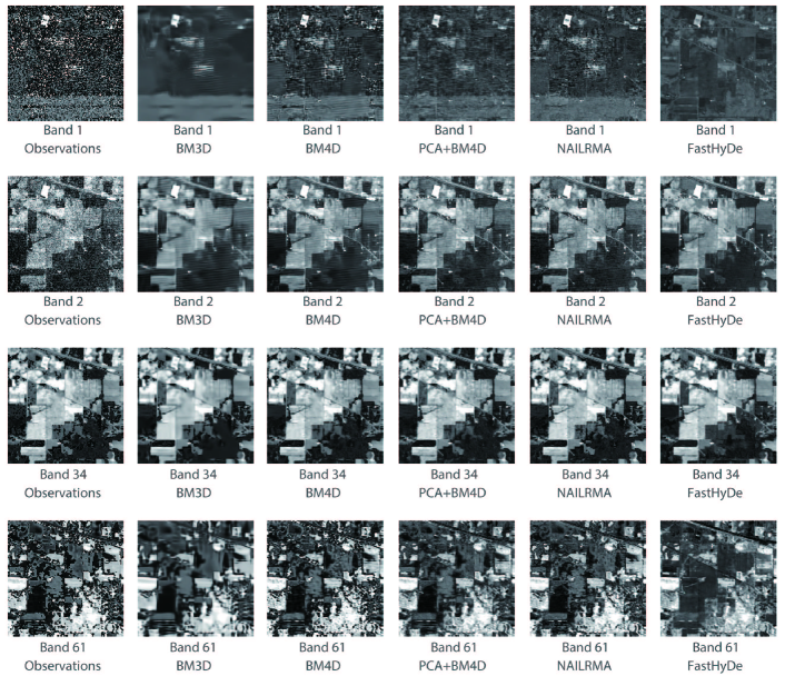
Figure 10: Denoising results of BM3D (75 s), BM4D (2934 s), PCA+BM4D (2761 s), NAILRMA (11 s) and FastHyDe (10 s) in Indian Pine data.

In this section we apply FastHyde to the AVIRIS (airborne visible/infrared imaging spectrometer) Indian Pines scene (Fig. 9-(a)) [48]. This image, recorded over North-western Indiana in June 1992, has $145\times 145$ pixels, with a spatial resolution of 20 meters per pixel and 220 spectral channels. The image displays strong noise in a number of bands. The noise was assumed to be non-i.i.d. and estimated with HySime. The first column in Fig. 10 shows four of those noise bands (1, 2, 34, and 61).

Indian Pine image was denoised by BM3D, BM4D, ‘PCA+BM4D’, NAILRMA and FastHyDe. The parameters used in BM3D and BM4D were set as in the simulated data. The subspace dimension input to ‘PCA+BM4D’ was 18, which is estimated by HySime [16]. Considering FastHyDe is robust to subspace dimension overestimation, subspace dimension input to FastHyDe was set to 25. The results are exhibited in Fig. 10 and the corresponding computational times are reported in the figure caption. Qualitatively, FastHyDe yields the best result, in the shortest time.

V-B Inpainting experiments

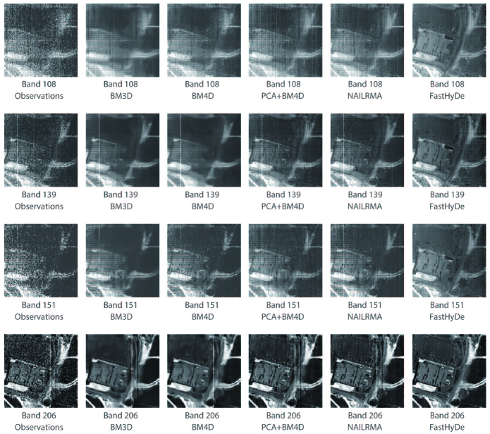
Figure 11: Denoising results of BM3D (64 s), BM4D (2579 s), PCA+BM4D (2405 s), NAILRMA (10 s) and FastHyDe (9 s) in Urban subscene.

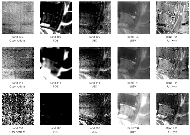
Figure 12: Inpainting results of PDE (86 s), UBD (5 s), LRTV (59 s) and FastHyIn (9 s) in Urban subscene.

We apply FastHyIn to Urban subscene (Fig. 9-(b)), which has $130\times 130$ pixels, with a spatial resolution of 2 meters per pixel and 210 spectral channels ranging from 400 nm to 2500 nm. Due to dense water vapor and atmospheric effects, the image displays strong noise in a number of bands. First column in Fig. 11 shows four of those noise bands (208, 139, 151, and 206).

We applied BM3D, BM4D, ‘PCA+BM4D’, NAILRMA and FastHyDe denoisers, under the assumption the noise is non-i.i.d. The parameters used in BM3D and BM4D were set to the same values as in the simulated data. The subspace dimension input to ‘PCA+BM4D’ was 6, which is estimated by HySime [16]. Considering FastHyDe is robust to subspace dimension overestimation, subspace dimension input to FastHyDe was set to 15. For NAILRMA, the block size and step size were set to 20 and 8, respectively. Denoising results are given in Fig. 11. Visually, FastHyDe recovers more information in these noisy bands than others do. On the other hand, a number of bands in Urban data contain almost no useful information, as shown in first column of Fig. 12. These bands were inpainted by FastHyIn, PDE, UBD, and LRTV. The parameters of LRTV were manually tuned as $r=6,~{}\tau=0.015,~{}\lambda=10^{5}$. The subspace dimension in FastHyIn was set to 15. As shown in 12, the inpainting results of FastHyIn are qualitatively better than those of other inpainters.

VI Conclusions

In this paper, we have proposed a new denoising method for HSIs, termed Fast Hyperspectral denoising (FastHyDe) and its extended version for inpainting, termed Fast Hyperspectral inpainting (FastHyIn). The new methods exploit two characteristics of HSIs: a) they live in low dimensional subspaces, and b) their images of subspace representation coefficients, herein termed eigen-images, are self-similar and thus suitable to be denoised with non-local patch-based methods. A comparison of FastHyDe and FastHyIn with the state-of-the-art algorithms is conducted, leading to the conclusion that FastHyDe and FastHyIn yield similar or better performance for additive noise and for Poissonian noise, with much lower computational complexity. FastHyDe and FastHyIn are not only fast, but also robust to subspace overestimation, and user-friendly, requiring no parameters, hard to tune. These characteristics put FastHyDe and FastHyIn in a privileged position to be used as an HSI denoiser and inpainter.

Lina Zhuang (S’15) received Bachelor’s degrees in geographic information system and in economics from South China Normal University, Ghuangzhou, China, in 2012, and the M.S. degree in cartography and geography information system from Institute of Remote Sensing and Digital Earth, Chinese Academy of Sciences, Beijing, China, in 2015. She is currently working toward the Ph.D. degree in Electrical and Computer Engineering at the Instituto Superior Técnico, Universidade de Lisboa, Lisbon, Portugal. Since 2015, she has been with the Instituto de Telecomunicações, as a Marie Curie Early Stage Researcher of Sparse Representations and Compressed Sensing Training Network (SpaRTaN number 607290). SpaRTaN Initial Training Networks (ITN) is funded under the European Union’s Seventh Framework Programme (FP7-PEOPLE-2013-ITN) call and is part of the Marie Curie Actions–ITN funding scheme. Her research interests include hyperspectral image denoising, inpainting, superresolution, and compressive sensing.

José M. Bioucas-Dias (S’87–M’95–SM’15–F’17) received the E.E., M.Sc., Ph.D., and Habilitation degrees in electrical and computer engineering from Instituto Superior Técnico (IST), Universidade Técnica de Lisboa (now Universidade de Lisboa), Portugal, in 1985, 1991, 1995, and 2007, respectively. Since 1995, he has been with the Department of Electrical and Computer Engineering, IST, where he is currently a Professor and teaches inverse problems in imaging and electric communications. He is also a Senior Researcher with the Pattern and Image Analysis group, Instituto de Telecomunicações, which is a private nonprofit research institution. His research interests include inverse problems, signal and image processing, pattern recognition, optimization, and remote sensing. He has introduced scientific contributions in the areas of imaging inverse problems, statistical image processing, optimization, phase estimation, phase unwrapping, and in various imaging applications, such as hyperspectral and radar imaging. Prof. Bioucas-Dias was included in Thomson Reuters’ Highly Cited Researchers 2015 list and was the recipient of the IEEE GRSS David Landgrebe Award for 2017.

References

- [1] J. Bioucas-Dias, A. Plaza, N. Dobigeon, M. Parente, Q. Du, P. Gader, and J. Chanussot, “Hyperspectral unmixing overview: Geometrical, statistical, and sparse regression-based approaches,” IEEE Journal of Selected Topics in Applied Earth Observations and Remote Sensing, vol. 5, no. 2, pp. 354–379, Apr. 2012.
- [2] N. Acito, M. Diani, and G. Corsini, “Signal-dependent noise modeling and model parameter estimation in hyperspectral images,” IEEE Transactions on Geoscience and Remote Sensing, vol. 49, no. 8, pp. 2957–2971, Aug. 2011.
- [3] M. L. Uss, B. Vozel, V. V. Lukin, and K. Chehdi, “Local signal-dependent noise variance estimation from hyperspectral textural images,” IEEE Journal of Selected Topics in Signal Processing, vol. 5, no. 3, pp. 469–486, Jun. 2011.
- [4] Y. Qian and M. Ye, “Hyperspectral imagery restoration using nonlocal spectral-spatial structured sparse representation with noise estimation,” IEEE Journal of Selected Topics in Applied Earth Observations and Remote Sensing, vol. 6, no. 2, pp. 499–515, Apr. 2013.
- [5] M. Makitalo and A. Foi, “A closed-form approximation of the exact unbiased inverse of the anscombe variance-stabilizing transformation,” IEEE Transactions on Image Processing, vol. 20, no. 9, pp. 2697–2698, Sep. 2011.
- [6] L. Zhuang and J. Bioucas-Dias, “Fast hyperspectral image denoising based on low rank and sparse representations,” in IEEE International Geoscience and Remote Sensing Symposium (IGARSS), Jul. 2016.
- [7] A. Buades, B. Coll, and J. M. Morel, “A non-local algorithm for image denoising,” in IEEE Computer Society Conference on Computer Vision and Pattern Recognition (CVPR), Jun. 2005, vol. 2, pp. 60–65 vol. 2.
- [8] A. M. Teodoro, M. S. C. Almeida, and M. A. T. Figueiredo, “Single-frame image denoising and inpainting using gaussian mixtures.,” in Proceedings of the International Conference on Pattern Recognition Applications and Methods (ICPRAM), Jan. 2015, pp. 283–288.
- [9] K. Dabov, A. Foi, V. Katkovnik, and K. Egiazarian, “Image denoising by sparse 3-d transform-domain collaborative filtering,” IEEE Transactions on Image Processing, vol. 16, no. 8, pp. 2080–2095, Aug. 2007.
- [10] M. Nejati, S. Samavi, S. Soroushmehr, and K. Najarian, “Low-rank regularized collaborative filtering for image denoising,” in IEEE International Conference on Image Processing (ICIP). IEEE, Sep. 2015, pp. 730–734.
- [11] D. Zoran and Y. Weiss, “From learning models of natural image patches to whole image restoration,” in IEEE International Conference on Computer Vision (ICCV), Nov. 2011, pp. 479–486.
- [12] M. Maggioni, V. Katkovnik, K. Egiazarian, and A. Foi, “Nonlocal transform-domain filter for volumetric data denoising and reconstruction,” IEEE Transactions on Image Processing, vol. 22, no. 1, pp. 119–133, Jan. 2013.
- [13] M. Maggioni, G. Boracchi, A. Foi, and K. Egiazarian, “Video denoising, deblocking, and enhancement through separable 4-D nonlocal spatiotemporal transforms,” IEEE Transactions on Image Processing, vol. 21, no. 9, pp. 3952–3966, Sep. 2012.
- [14] A. Danielyan, A. Foi, V. Katkovnik, and K. Egiazarian, “Denoising of multispectral images via nonlocal groupwise spectrum-PCA,” in Conference on Colour in Graphics, Imaging, and Vision. Society for Imaging Science and Technology, Jan. 2010, vol. 2010, pp. 261–266.
- [15] A. Rajwade, A. Rangarajan, and A. Banerjee, “Image denoising using the higher order singular value decomposition,” IEEE Transactions on Pattern Analysis and Machine Intelligence, vol. 35, no. 4, pp. 849–862, Apr. 2013.
- [16] J. Bioucas-Dias and J. Nascimento, “Hyperspectral subspace identification,” IEEE Transactions on Geoscience and Remote Sensing, vol. 46, no. 8, pp. 2435–2445, Aug. 2008.
- [17] W. He, H. Zhang, L. Zhang, and H. Shen, “Hyperspectral image denoising via noise-adjusted iterative low-rank matrix approximation,” IEEE Journal of Selected Topics in Applied Earth Observations and Remote Sensing, vol. 8, no. 6, pp. 3050–3061, Jun. 2015.
- [18] H. Zhang, W. He, L. Zhang, H. Shen, and Q. Yuan, “Hyperspectral image restoration using low-rank matrix recovery,” IEEE Transactions on Geoscience and Remote Sensing, vol. 52, no. 8, pp. 4729–4743, Aug. 2014.
- [19] W. He, H. Zhang, L. Zhang, and H. Shen, “Total-variation-regularized low-rank matrix factorization for hyperspectral image restoration,” IEEE Transactions on Geoscience and Remote Sensing, vol. 54, no. 1, pp. 178–188, Jan. 2016.
- [20] J. Li, Q. Yuan, H. Shen, and L. Zhang, “Noise removal from hyperspectral image with joint spectral-spatial distributed sparse representation,” IEEE Transactions on Geoscience and Remote Sensing, vol. 54, no. 9, pp. 5425–5439, Sep. 2016.
- [21] T. Lu, S. Li, L. Fang, Y. Ma, and J. A. Benediktsson, “Spectral-spatial adaptive sparse representation for hyperspectral image denoising,” IEEE Transactions on Geoscience and Remote Sensing, vol. 54, no. 1, pp. 373–385, Jan. 2016.
- [22] Q. Yuan, L. Zhang, and H. Shen, “Hyperspectral image denoising employing a spectral–spatial adaptive total variation model,” IEEE Transactions on Geoscience and Remote Sensing, vol. 50, no. 10, pp. 3660–3677, Oct. 2012.
- [23] H. Shen, X. Li, L. Zhang, D. Tao, and C. Zeng, “Compressed sensing-based inpainting of aqua moderate resolution imaging spectroradiometer band 6 using adaptive spectrum-weighted sparse bayesian dictionary learning,” IEEE Transactions on Geoscience and Remote Sensing, vol. 52, no. 2, pp. 894–906, Feb. 2014.
- [24] L. Fang, S. Li, X. Kang, and J. A. Benediktsson, “Spectral-spatial hyperspectral image classification via multiscale adaptive sparse representation,” IEEE Transactions on Geoscience and Remote Sensing, vol. 52, no. 12, pp. 7738–7749, 12 2014.
- [25] L. Fang, S. Li, X. Kang, and J. A. Benediktsson, “Spectral spatial classification of hyperspectral images with a superpixel-based discriminative sparse model,” IEEE Transactions on Geoscience and Remote Sensing, vol. 53, no. 8, pp. 4186–4201, Aug. 2015.
- [26] L. Fang, C. Wang, S. Li, and J. A. Benediktsson, “Hyperspectral image classification via multiple-feature-based adaptive sparse representation,” IEEE Transactions on Instrumentation and Measurement, vol. 66, no. 7, pp. 1646–1657, Jul. 2017.
- [27] M. Bertalmio, G. Sapiro, V. Caselles, and C. Ballester, “Image inpainting,” in Proceedings of the 27th annual conference on Computer graphics and interactive techniques, 2002, pp. 417–424.
- [28] A. A. Efros and T. K. Leung, “Texture synthesis by non-parametric sampling,” in The Proceedings of the 7th IEEE International Conference on Computer Vision. IEEE, Sep. 1999, vol. 2, pp. 1033–1038.
- [29] M. Bertalmio, L. Vese, G. Sapiro, and S. Osher, “Simultaneous structure and texture image inpainting,” IEEE transactions on image processing, vol. 12, no. 8, pp. 882–889, Aug. 2003.
- [30] G. Aubert and P. Kornprobst, Mathematical problems in image processing: partial differential equations and the calculus of variations, vol. 147, Springer Science & Business Media, Nov. 2006.
- [31] T. F. Chan, J. Shen, and H.-M. Zhou, “Total variation wavelet inpainting,” Journal of Mathematical imaging and Vision, vol. 25, no. 1, pp. 107–125, Jul. 2006.
- [32] H. Shen and L. Zhang, “A MAP-based algorithm for destriping and inpainting of remotely sensed images,” IEEE Transactions on Geoscience and Remote Sensing, vol. 47, no. 5, pp. 1492–1502, May 2009.
- [33] A. Criminisi, P. Pérez, and K. Toyama, “Region filling and object removal by exemplar-based image inpainting,” IEEE Transactions on image processing, vol. 13, no. 9, pp. 1200–1212, Sep. 2004.
- [34] F. Melgani, “Contextual reconstruction of cloud-contaminated multitemporal multispectral images,” IEEE Transactions on Geoscience and Remote Sensing, vol. 44, no. 2, pp. 442–455, Feb. 2006.
- [35] A.-B. Salberg, “Land cover classification of cloud-contaminated multitemporal high-resolution images,” IEEE Transactions on Geoscience and Remote Sensing, vol. 49, no. 1, pp. 377–387, Jan. 2011.
- [36] Q. Cheng, H. Shen, L. Zhang, and P. Li, “Inpainting for remotely sensed images with a multichannel nonlocal total variation model,” IEEE Transactions on Geoscience and Remote Sensing, vol. 52, no. 1, pp. 175–187, Jan. 2014.
- [37] P. Combettes and V. Wajs, “Signal recovery by proximal forward-backward splitting,” Multiscale Modeling & Simulation, vol. 4, no. 4, pp. 1168–1200, 2005.
- [38] S. V. Venkatakrishnan, C. A. Bouman, and B. Wohlberg, “Plug-and-play priors for model based reconstruction,” in IEEE Global Conference on Signal and Information Processing, Dec. 2013, pp. 945–948.
- [39] A. Teodoro, J. Bioucas-Dias, and M. Figueiredo, “Sharpening hyperspectral images using plug-and-play priors,” in International Conference on Latent Variable Analysis and Signal Separation. Springer, Feb. 2017, pp. 392–402.
- [40] M. Ljubenović and M. A. T. Figueiredo, “Blind image deblurring using class-adapted image priors,” in IEEE International Conference on Image Processing (ICIP), 2017.
- [41] G. Chen, T. Bui, K. Quach, and S.-E. Qian, “Denoising hyperspectral imagery using principal component analysis and block-matching 4D filtering,” Canadian Journal of Remote Sensing, vol. 40, no. 1, pp. 60–66, Jan. 2014.
- [42] F. Anscombe, “The transformation of poisson, binomial and negative-binomial data,” Biometrika, pp. 246–254, Dec. 1948.
- [43] J. D’Errico, “Inpainting nan elements in 3-D,” 2008, MATLAB Central File Exchange, MathWorks, Natick, MA, USA (Available: www.mathworks.com/matlabcentral/fileexchange/21214-inpainting-nan-elements-in-3-d).
- [44] D. Cerra, R. Muller, and P. Reinartz, “Unmixing-based denoising for destriping and inpainting of hyperspectral images,” in IEEE International Geoscience and Remote Sensing Symposium (IGARSS), Jul. 2014, pp. 4620–4623.
- [45] J. Nascimento and J. Bioucas-Dias, “Vertex component analysis: a fast algorithm to unmix hyperspectral data,” IEEE Transactions on Geoscience and Remote Sensing, vol. 43, no. 4, pp. 898–910, Apr. 2005.
- [46] N. Keshava and J. F. Mustard, “Spectral unmixing,” IEEE signal processing magazine, vol. 19, no. 1, pp. 44–57, Jan. 2002.
- [47] A. Plaza, J. A. Benediktsson, J. W. Boardman, J. Brazile, L. Bruzzone, G. Camps-Valls, J. Chanussot, M. Fauvel, P. Gamba, A. Gualtieri, M. Marconcinie, J. C. Tiltoni, and G. Triannih, “Recent advances in techniques for hyperspectral image processing,” Remote sensing of environment, vol. 113, pp. S110–S122, Sep. 2009.
- [48] M. F. Baumgardner, L. L. Biehl, and D. A. Landgrebe, “220 band aviris hyperspectral image data set: June 12, 1992 Indian Pine test site 3,” Purdue University Research Repository, 2015.