Nontrivial damping of quantum many-body dynamics

Abstract

Understanding how the dynamics of a given quantum system with many degrees of freedom is altered by the presence of a generic perturbation is a notoriously difficult question. Recent works predict that, in the overwhelming majority of cases, the unperturbed dynamics is just damped by a simple function, e.g., exponentially as expected from Fermi’s golden rule. While these predictions rely on random-matrix arguments and typicality, they can only be verified for a specific physical situation by comparing to the actual solution or measurement. Crucially, it also remains unclear how frequent and under which conditions counterexamples to the typical behavior occur. In this work, we discuss this question from the perspective of projection-operator techniques, where exponential damping of a density matrix occurs in the interaction picture but not necessarily in the Schrödinger picture. We show that a nontrivial damping in the Schrödinger picture can emerge if the dynamics in the unperturbed system possesses rich features, for instance due to the presence of strong interactions. This suggestion has consequences for the time dependence of correlation functions. We substantiate our theoretical arguments by large-scale numerical simulations of charge transport in the extended Fermi-Hubbard chain, where the nearest-neighbor interactions are treated as a perturbation to the integrable reference system.

I Introduction

Questions of equilibration and thermalization in isolated quantum systems have experienced a renaissance in recent years D’Alessio et al. (2016); Borgonovi et al. (2016); Gogolin and Eisert (2016). However, notwithstanding the significant progress that has been made Paeckel et al. (2019), describing the precise dynamics of a given quantum many-body system still remains a very challenging task. “Universal” principles, which provide a faithful understanding of a wide class of models in various nonequilibrium situations, are therefore highly desirable Dziarmaga (2010); Polkovnikov et al. (2011); Erne et al. (2018); Prüfer et al. (2018); Reimann et al. (2020); Alhambra et al. (2020). A particularly successful strategy in this context has been the usage of random-matrix ensembles which mimic certain aspects of the full many-body problem Brody et al. (1981). Prominent examples include the eigenstate thermalization hypothesis Deutsch (1991); Srednicki (1994); Rigol et al. (2008), which asserts that the matrix structure of observables becomes essentially random in the eigenbasis of chaotic Hamiltonians Khaymovich et al. (2019); Richter et al. (2020a); Schönle et al. (2021); Brenes et al. (2021), as well as random-circuit models von Keyserlingk et al. (2018); Nahum et al. (2018); Khemani et al. (2018), which have led to new insights into the emergence of hydrodynamics and information scrambling in isolated quantum systems.

A particularly intriguing and omnipresent question in physics is how the dynamics of a given quantum system is affected by the presence of a perturbation Deutsch (1991); Knipschild and Gemmer (2018); Nation and Porras (2019); Dabelow and Reimann (2020a, 2021); Richter et al. (2020b), i.e., scenarios where the Hamiltonian ${\cal H}$ of the full system can be written as

$${\cal H}={\cal H}_{0}+\varepsilon{\cal V}\ ,$$ (1)

with ${\cal H}_{0}$ being an unperturbed reference system and $\varepsilon$ denoting the strength of the perturbation ${\cal V}$. This includes, e.g., the phenomenon of prethermalization Berges et al. (2004); Moeckel and Kehrein (2008); Bertini et al. (2015); Mori et al. (2018); Reimann and Dabelow (2019); Mallayya et al. (2019), where ${\cal V}$ weakly breaks a conservation law of the (usually integrable) ${\cal H}_{0}$, and also the analysis of imperfect echo protocols Schmitt and Kehrein (2018); Dabelow and Reimann (2020b), where the respective Hamiltonians governing the forward and backward time evolutions are different. In an even broader context, the impact of perturbations also plays an important role for simulations on today’s noisy intermediate-scale quantum devices Preskill (2018), where ${\cal V}$ can be interpreted as the inevitable imperfections of elementary gates which alter the desired circuit Arute et al. (2019).

Given a quantum system with many degrees of freedom, the impact of a perturbation can clearly be manifold. It is therefore quite remarkable that a series of recent works predict that, in the overwhelming majority of cases, the reference dynamics is just damped by a simple function Dabelow and Reimann (2020a, 2021), e.g., exponentially as expected from Fermi’s golden rule Genway et al. (2013); Richter et al. (2020b); Werner et al. (2020). In essence, these works rely on random-matrix theory as ${\cal V}$ is modeled by (an ensemble of) random matrices with respect to the eigenstates of ${\cal H}_{0}$ Dabelow and Reimann (2020a), as well as on the concept of typicality Popescu et al. (2006); Goldstein et al. (2006); Bartsch et al. (2008); Reimann (2018), as a given perturbation is shown to behave very similar to the ensemble average. However, while these predictions were found to compare favorably to a variety of experimental and numerical examples Dabelow and Reimann (2020a), it yet remains unclear how frequent and under which conditions counterexamples to the typical behavior occur.

In this work, we discuss exactly this question from the perspective of projection-operator techniques, which are well established in the realm of open quantum systems Breuer and Petruccione (2007). In this way, we provide a fresh insight and show that, within these techniques and under mild assumptions, the “standard” case of exponential damping emerges for the density matrix in the interaction picture but not necessarily in the Schrödinger picture. We particularly suggest that a nontrivial damping in the Schrödinger picture can emerge if the dynamics in the unperturbed system possesses rich features. This suggestion has consequences for the time dependence of correlation functions. It is substantiated by large-scale numerical simulations of charge transport in the extended Fermi-Hubbard chain, where the nearest-neighbor interactions are treated as a perturbation to the integrable reference system.

This paper is structured as follows. In Sec. II we first establish the setup by introducing an exemplary model and observable, and then turn to a description of our projection-operator approach and its implications on the relaxation dynamics in perturbed many-body quantum systems. We show illustrating numerical results in Sec. III and conclude in Sec. IV.

II Setup and projection-operator approach

II.1 Model and observable

Even though our analytical reasoning can be applied to arbitrary operators and Hamiltonians, we here consider for concreteness the dynamics of the particle current in the extended Fermi-Hubbard chain, which constitutes a physically relevant many-body quantum problem (see Refs. Zotos and Prelovšek (2004); Bertini et al. (2021); Bulchandani et al. (2021) and references therein). The Hamiltonian of this model reads ${\cal H}=\sum_{r=1}^{L}h_{r}$ and is a sum over $L$ local terms

$$h_{r}= - t_{\text{h}}\sum_{\sigma=\uparrow,\downarrow}(c_{r,\sigma}^{\dagger}c_{r+1,\sigma}^{\phantom{\dagger}}+\text{H.c.})+U(n_{r,\uparrow}-\tfrac{1}{2})(n_{r,\downarrow}-\tfrac{1}{2})$$ (2)

$$+ U^{\prime}\sum_{\sigma,\sigma^{\prime}}(n_{r,\sigma}-\tfrac{1}{2})(n_{r+1,\sigma^{\prime}}-\tfrac{1}{2})\,,$$

where we assume periodic boundary conditions, i.e., we have $L+1\equiv 1$. $c_{r,\sigma}^{\dagger}$ ($c_{r,\sigma}^{\phantom{\dagger}}$) creates (annihilates) a fermion with spin $\sigma$ at lattice site $r$ and $n_{r,\sigma}=c_{r,\sigma}^{\dagger}c_{r,\sigma}^{\phantom{\dagger}}$ is the occupation-number operator. $t_{\text{h}}$ is the hopping matrix element and $U,U^{\prime}>0$ denote the strengths of the repulsive on-site and nearest-neighbor interactions, respectively. While the model is noninteracting for $U,U^{\prime}=0$, it in fact remains integrable in terms of the Bethe ansatz also for finite on-site interactions $U>0$ Essler et al. (2005). In contrast, this integrability is broken for any $U^{\prime}>0$. Note that ${\cal H}$ preserves the number of each fermion species.

As an observable, we consider the particle current. It can be derived from a continuity equation and takes on the well-known form (see Refs. Zotos and Prelovšek (2004); Bertini et al. (2021); Bulchandani et al. (2021) and references therein) ${\cal J}=\sum_{r=1}^{L}j_{r}$,

$$j_{r}=-t_{\text{h}}\sum_{\sigma=\uparrow,\downarrow}[(i\,c_{r,\sigma}^{\dagger}c_{r+1,\sigma}^{\phantom{\dagger}}+\text{H.c.})]\,.$$ (3)

While the particle current does not depend on $U$ and $U^{\prime}$, its dynamics does. Only in the case $U=U^{\prime}=0$, we have $[{\cal J},{\cal H}]=0$. Generally, $\text{tr}[{\cal J}]=0$ and $\text{tr}[{\cal J}^{2}]=DLt_{\text{h}}^{2}/4$, where $D=4^{L}$ is the dimension of the Hilbert space. In this paper, we will be particularly concerned with the dynamics of current-current correlation functions. However, as already stated above, all that follows now carries over to other choices of observable and Hamiltonian.

II.2 Projection-operator approach

To apply projection-operator techniques, we first decompose the full system $\cal H$ according to Eq. (1) into an unperturbed system ${\cal H}_{0}$ and a perturbation $\varepsilon\,\cal V$. For instance, for the Fermi-Hubbard chain (2), we will later consider two different reference systems ${\cal H}_{0}$, i.e., the noninteracting ${\cal H}_{0}={\cal H}(U=U^{\prime}=0)$ and the interacting integrable ${\cal H}_{0}={\cal H}(U\neq 0,U^{\prime}=0)$.

After this decomposition, we then define a projection superoperator ${\cal P}$, which projects a density matrix $\rho(t)$ at time $t$ onto a set of relevant degrees of freedom. This set should at least include the identity and the observable of interest,

$${\cal P}\,\rho(t)=\frac{1}{D}+\frac{C(t)}{\langle{\cal J}^{2}\rangle}\,{\cal J}\,,\quad C(t)=\langle{\cal J}\rho(t)\rangle\,,$$ (4)

where $\langle\bullet\rangle=\text{tr}[\bullet]/D$. Due to $\langle{\cal J}\rangle=0$, ${\cal P}^{2}={\cal P}$. In this work, we are interested in the time-dependent part $C(t)$ of the projected density matrix. It is important to note that, using the projection in Eq. (4), $C(t)$ is not identical in the Schrödinger and interaction picture. Even though $C(t)$ is a coefficient and not an expectation value, it will turn out below that $C(t)$ can be expressed in terms of certain types of correlation functions. Importantly, throughout this paper, the notions of Schrödinger or interaction picture should be understood with respect to the dynamics of the density matrix. This wording should not be confused with the fact that expectation values of observables are the same in both pictures.

While taking into account more degrees of freedom is possible, this will not be necessary for our purposes. In particular, for initial conditions $\rho(0)$ in the span of $1$ and $\cal J$, we further have ${\cal P}\rho(0)=\rho(0)$. From now on, we will focus on such kind of initial conditions, which also appear in the context of linear response theory LRT .

After having defined the projection superoperator (and the reference system), the so-called time-convolutionless (TCL) projection-operator technique routinely leads to a time-local differential equation for the evolution of ${\cal P}\rho_{\text{I}}(t)$ in the interaction picture Breuer and Petruccione (2007); Chaturvedi and Shibata (1979),

$$\frac{\partial}{\partial t}{\cal P}\rho_{\text{I}}(t)={\cal G}(t)\,{\cal P}\rho_{\text{I}}(t)+{\cal I}(t)\,(1-{\cal P})\,\rho(0)\,,$$ (5)

where $\rho_{\text{I}}(t)=e^{i{\cal H}_{0}t}e^{-i{\cal H}t}\rho(0)e^{i{\cal H}t}e^{-i{\cal H}_{0}t}$. The term ${\cal I}(t)$, i.e., the inhomogeneity on the right hand side (r.h.s.) of Eq. (5), can be neglected, due to $(1-{\cal P})\,\rho(0)=0$. The generator ${\cal G}(t)$ is given as a systematic series expansion in powers of $\varepsilon$. In many cases, just like in our case, odd orders vanish. Hence, the lowest order is the second order and reads

$${\cal G}_{2}(t)=\varepsilon^{2}\!\int_{0}^{t}\!\text{d}t^{\prime}\,{\cal P}{\cal L}(t){\cal L}(t^{\prime}){\cal P}\,,$$ (6)

where the Liouvillian is given by ${\cal L}(t)\,\bullet=-i[{\cal V}_{\text{I}}(t),\bullet]$ with ${\cal V}_{\text{I}}(t)=e^{i{\cal H}_{0}t}\,{\cal V}(0)\,e^{-i{\cal H}_{0}t}$.

So far, we have invoked no significant assumption. The central assumption in the following will be a truncation to lowest order. The quality of such a truncation naturally depends on the perturbation strength $\varepsilon$, but also on the structure of the perturbation $\cal V$ and the degrees of freedom in the projection superoperator $\cal P$. Note, however, that a truncation to lowest order does not necessarily imply that we have to restrict ourselves to weak perturbations $\varepsilon\rightarrow 0$ and long times $t\rightarrow\infty$. In particular, a lowest-order truncation turns out to be reasonable in many situations Bartsch et al. (2008). While the quality can naturally be further improved by taking into account higher-order corrections Steinigeweg (2011), conditions for neglecting higher orders at rather large $\varepsilon$ can be found in Ref. Steinigeweg (2011).

Now, we use a truncation to lowest order, as well as the simple mathematical facts that,

$$C(t)\propto\langle{\cal J}(t){\cal J}\rangle\ ,\quad C_{\text{I}}(t)\propto\langle{\cal J}(t){\cal J}_{\text{I}}(t)\rangle\ ,$$ (7)

which relate the time-dependent part of the density matrix (in the Schrödinger or interaction picture) to a certain type of correlation function. (A derivation of this relation can be found in Appendix C.) In particular, within the TCL formalism, a rate equation can be obtained for $C_{\text{I}}(t)$ in the interaction picture,

$$\frac{\partial}{\partial t}\langle{\cal J}(t){\cal J}_{\text{I}}(t)\rangle=-\varepsilon^{2}\,\gamma_{2}(t)\,\langle{\cal J}(t){\cal J}_{\text{I}}(t)\rangle\,,$$ (8)

where ${\cal J}(t)=e^{i{\cal H}t}\,{\cal J}(0)\,e^{-i{\cal H}t}$ and the time-dependent damping $\gamma_{2}(t)$ results from a time-integral over a kernel $k_{2}(t,t^{\prime})=k_{2}(\tau=t-t^{\prime})$,

$$\gamma_{2}(t)=\int_{0}^{t}\!\!\text{d}\tau\,k_{2}(\tau)\,,\,k_{2}(\tau)=\frac{\langle i[{\cal J},{\cal V}_{\text{I}}(\tau)]i[{\cal J},{\cal V}_{\text{I}}]\rangle}{\langle\mathcal{J}^{2}\rangle}\,.$$ (9)

Apparently, if $k_{2}(\tau)\to 0$ for sufficiently long times, then we have $\gamma_{2}(t)\to\text{const.}$ at such time scales. We note that the kernel $k_{2}(\tau)$ can in principle be calculated analytically in the thermodynamic limit, if the reference system ${\cal H}_{0}$ is integrable. But often a numerical calculation of $k_{2}(\tau)$ in systems of finite size is sufficient Steinigeweg (2011).

The solution of rate equation (8) obviously is an exponential decay of the form

$$\frac{\langle{\cal J}(t){\cal J}_{\text{I}}(t)\rangle}{\langle{\cal J}^{2}\rangle}=\exp\Big{[}-\varepsilon^{2}\!\int_{0}^{t}\!\text{d}t^{\prime}\,\gamma_{2}(t^{\prime})\Big{]}\,.$$ (10)

This solution reflects our central result: Within our TCL approach, the time-dependent part of the density matrix is damped exponentially in the interaction picture and not necessarily in the Schrödinger picture. Clearly, both pictures must agree, if the observable $\cal J$ is preserved in the reference system ${\cal H}_{0}$, $[{\cal J},{\cal H}_{0}]=0$. For instance, for the particle current in the Fermi-Hubbard chain, this preservation is given in the noninteracting ${\cal H}_{0}={\cal H}(U=U^{\prime}=0)$. Therefore, both pictures can also be expected to be rather similar, whenever the dynamics of ${\cal J}_{\text{I}}(t)$ is sufficiently slow compared to the dynamics of ${\cal J}(t)$. In the general situation, however, the two pictures are just not the same:

$$\frac{\langle{\cal J}(t){\cal J}\rangle_{\varepsilon>0}}{\langle{\cal J}(t){\cal J}\rangle_{\varepsilon=0}}\neq\frac{\langle{\cal J}(t){\cal J}_{\text{I}}(t)\rangle}{\langle{\cal J}^{2}\rangle}\,.$$ (11)

Hence, a priori, one cannot expect that the lowest-order prediction of an exponential decay in Eq. (10) simply carries over to the Schrödinger picture, and the relaxation dynamics of $\langle{\cal J}(t){\cal J}\rangle_{\varepsilon>0}$ may exhibit nontrivial behavior that is distinct from typicality predictions in Refs. Dabelow and Reimann (2020a, 2021). For instance, as we demonstrate later, this difference is eye striking for the strongly interacting reference system ${\cal H}_{0}={\cal H}(U\gg t_{\text{h}},U^{\prime}=0)$. Note that Eq. (10) has also consequences for transport quantities.

III Numerical illustration

Next, we illustrate our central result in numerical simulations after a description of the employed method.

III.1 Method

To study system sizes larger than what is possible with full exact diagonalization (ED), we rely on the concept of dynamical quantum typicality (DQT) Popescu et al. (2006); Goldstein et al. (2006); Bartsch and Gemmer (2009); Reimann (2018) and obtain time-dependent autocorrelation functions from a single pure state $|\psi\rangle$, which is drawn at random from a high-dimensional Hilbert space. While this approach is by now well established for “standard” correlation functions such as $\langle{\cal J}(t){\cal J}\rangle$ (see Refs. Jin et al. (2021); Heitmann et al. (2020) and references therein), the dynamics of correlation functions with a more complicated time dependence such as $\langle{\cal J}(t){\cal J}_{\text{I}}(t)\rangle$ can be obtained in a rather similar fashion. Specifically, we first introduce the two auxiliary pure states

$$|\phi(t)\rangle = e^{-i{\cal H}t}\,e^{i{\cal H}_{0}t}\,|\psi\rangle\,,$$ (12)

$$|\varphi(t)\rangle = e^{-i{\cal H}t}\,e^{i{\cal H}_{0}t}\,{\cal J}\,|\psi\rangle\,,$$ (13)

and then approximate the autocorrelation function and its time dependence as

$$\langle{\cal J}(t){\cal J}_{\text{I}}(t)\rangle=\frac{\langle\phi(t)|{\cal J}|\varphi(t)\rangle}{\langle\phi|\phi\rangle}+{\cal O}\Big{(}\frac{1}{\sqrt{D}}\Big{)}\,,$$ (14)

where the statistical error becomes negligibly small for system sizes studied here. Compared to the usual approximation of $\langle{\cal J}(t){\cal J}\rangle$ Iitaka and Ebisuzaki (2003); Elsayed and Fine (2013), the approximation of $\langle{\cal J}(t){\cal J}_{\text{I}}(t)\rangle$ is more costly from a numerical point of view, since at each point in time an additional backward propagation with respect to the reference system ${\cal H}_{0}$ is required. However, this extra operation can still be carried out in large Hilbert spaces beyond the range of full ED, thereby reducing the impact of finite-size effects, see Appendix B for a detailed analysis of finite-size effects. In this paper, we treat systems with up to $L=16$, where $D\approx 4.3\times 10^{9}$, and the largest symmetry subspace has a dimension $\approx 10^{7}$. Note that a time evolution of the form (12) is also relevant for the stability of quantum motion with respect to a static perturbation Prosen and Žnidarič (2002).

III.2 Results

Let us now turn to our actual numerical results for the two scenarios of a noninteracting and an interacting reference system.

III.2.1 Noninteracting reference system

Figure 1: (a) Decay of the current autocorrelation function $\langle\mathcal{J}(t)\mathcal{J}\rangle$ for the noninteracting ${\cal H}_{0}={\cal H}(U=U^{\prime}=0)$, which is perturbed by particle-particle interactions of various strengths $U/t_{\text{h}}=U^{\prime}/t_{\text{h}}=\varepsilon\leq 4$. Numerical results from DQT in a finite system of size $L=16$ are compared to the lowest-order prediction of the TCL projection-operator technique in Eq. (10). (b) Kernel $k_{2}(t)$ and (c) rate $\gamma_{2}(t)$, as both given in Eq. (9), for $L\leq 16$. Finite-size effects are mild and systematic. The expected plateau value of $\gamma_{2}(t)$ for $L\to\infty$ is indicated (dash-dotted line).

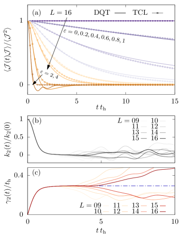
We start with a decomposition where the reference system is chosen to be noninteracting, ${\cal H}_{0}={\cal H}(U=U^{\prime}=0)$, such that Schrödinger and interaction picture are identical, $C(t)=C_{\text{I}}(t)$, due to $[{\cal J},{\cal H}_{0}]=0$. The role of the perturbation is then played by the particle-particle interaction terms. In Fig. 1, we summarize the decay of the current autocorrelation function $\langle{\cal J}(t){\cal J}\rangle=\langle{\cal J}(t){\cal J}_{\text{I}}(t)\rangle$ for a finite system of size $L=16$ and interaction strengths $U/t_{\text{h}}=U^{\prime}/t_{\text{h}}=\varepsilon\leq 4$. The decay is faster the larger $\varepsilon$, and an exponential relaxation for weak $\varepsilon$ changes into a Gaussian type of relaxation for stronger $\varepsilon$. This overall behavior is in qualitative agreement with the lowest-order prediction of the TCL projection-operator technique in Eq. (10). Note that the Gaussian behavior is expected due to $\gamma_{2}(t)\propto t$ at small $t$, which become relevant for large $\varepsilon$ Steinigeweg (2011).

To exclude that this agreement is accidental, we depict in Figs. 1(b) and 1(c) numerical results for the kernel $k_{2}(t)$ and rate $\gamma_{2}(t)$, as both given in Eq. (9), for different chain lengths $L\leq 16$. Apparently, $k_{2}(t)$ decays fast to zero, and the visible finite-size effects set in at time scales after this initial decay. As a consequence, the damping $\gamma_{2}(t)$ shows a mild dependence on system size and, in particular, a conclusion on the plateau value of $\gamma_{2}(t)$ for $L\to\infty$ is possible. Therefore, we can quantitatively evaluate the lowest-order prediction in Eq. (10) and compare to the direct numerics in Fig. 1 discussed before. We find that the agreement is remarkably good over a wide range of perturbation strengths $\varepsilon$, and small differences might be either related to residual finite-size effects or missing higher-order corrections. A detailed analysis of finite-size effects can be found in Appendix B. Thus, our TCL approach correctly captures the “standard” case of exponential damping of $\langle{\cal J}(t){\cal J}\rangle$, in agreement with typicality and random-matrix considerations Dabelow and Reimann (2020a, 2021); Richter et al. (2020b).

III.2.2 Interacting reference system

Figure 2: Decay of (a) $C(t)=\langle\mathcal{J}(t)\mathcal{J}\rangle$ and (b) $C_{\text{I}}(t)=\langle\mathcal{J}(t)\mathcal{J}_{\mathrm{I}}(t)\rangle$ for the interacting $\mathcal{H}_{0}=\mathcal{H}(U/t_{\text{h}}=16,U^{\prime}=0)$, which is perturbed in this case by nearest-neighbor particle-particle interactions of strength $U^{\prime}/t_{\text{h}}=\varepsilon\leq 2$. Numerical results from DQT are shown for a finite system of size $L=12$ and in (b) additionally compared to the lowest-order prediction of the TCL projection-operator technique in Eq. (10). For the kernel $k_{2}(t)$ and rate $\gamma_{2}(t)$, see Fig. 5 in Appendix B. The inset in (a) shows the ratio between $\langle{\cal J}(t){\cal J}\rangle_{\varepsilon>0}$ (perturbed dynamics) and $\langle{\cal J}(t){\cal J}\rangle_{\varepsilon=0}$ (unperturbed dynamics) in the Schrödinger picture. This ratio is a nontrivial function and does not coincide with the damping in the interaction picture.

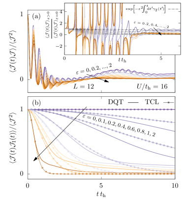
Finally, and most importantly in the context of this paper, we turn to the decomposition ${\cal H}={\cal H}_{0}+\varepsilon{\cal V}$ with an interacting reference system, $\mathcal{H}_{0}=\mathcal{H}(U\neq 0,U^{\prime}=0)$, where the Schrödinger and interaction picture are no longer the same, $C(t)\neq C_{I}(t)$, and the perturbation ${\cal V}$ is given by the nearest-neighbor interaction $U^{\prime}>0$. We decide to choose a large on-site interaction $U/t_{\text{h}}=16\gg 1$, since the dynamics for such $U$ is known to have rich features Karrasch et al. (2014a); Jin et al. (2015). However, the overall phenomenology emerges for smaller values of $U$ as well, as can be seen in the additional data presented in Appendix A. As shown in Fig. 2(a) for a finite system size $L=12$, $C(t)=\langle{\cal J}(t){\cal J}\rangle$ in the Schrödinger picture exhibits oscillatory behavior, where the frequencies and zero crossings also vary with the strength $U^{\prime}/t_{\text{h}}=\varepsilon$ of the nearest-neighbor interaction. Hence, from visual inspection, it is clear that unperturbed and perturbed dynamics cannot be related by a simple damping function. Their nontrivial relation becomes even more obvious by plotting their ratio (see the inset of Fig. 2).

In the interaction picture, however, the situation turns out to be different. As shown in Fig. 2(b), the behavior of $C_{\text{I}}(t)=\langle{\cal J}(t){\cal J}_{\text{I}}(t)\rangle$ is like the one in Fig. 1. It decays monotonously and changes from exponential to Gaussian type of relaxation as $\varepsilon$ is increased, in qualitative agreement with the lowest-order prediction of the TCL projection-operator technique in Eq. (10). Furthermore, a quantitative comparison is also feasible, since the corresponding kernel $k_{2}(t)$ and rate $\gamma_{2}(t)$ are converged with respect to system size (see Fig. 7 in Appendix B), at least for the time scales depicted in Fig. 2(b). Apparently, the agreement is not as convincing as before and deviations set in for times $t\,t_{\text{h}}\sim 4$. However, for such times, the direct numerics is known to still depend on system size (see, e.g., Refs. Karrasch et al. (2014a); Jin et al. (2015) and Appendix B), and deviations might eventually disappear in the thermodynamic limit $L\to\infty$. We should also stress that the restriction by the finite-size time $t\,t_{\text{h}}\sim 4$ does not allow us to study very weak perturbations $\varepsilon\ll 0.1$ in our numerical simulation, where the relaxation takes place on a much longer time scale. How to numerically study the limit of very weak $\varepsilon$ therefore remains an open problem.

In the specific context of currents, this result also has direct consequences for the transport behavior Zotos (2004); Jung et al. (2006); Steinigeweg et al. (2016); i.e., only in the interaction picture is the dynamics of the density matrix exponentially damped due to perturbations such that (i) the frequency dependence of the conductivity has a simple Lorentzian form and (ii) the dc conductivity $\sigma_{\text{dc}}$ scales as $\sigma_{\text{dc}}\propto 1/\varepsilon^{2}$. But for the dynamics of the density matrix in the Schrödinger picture, which is of actual interest, both (i) and (ii) cannot be expected (see also the corresponding data shown in Appendix D).

IV Conclusion

We have addressed the question of how the dynamics of a given quantum system is altered when a perturbation is switched on. We have shown that, within our analytical approach based on projection-operator techniques, the “standard” case of exponential damping occurs for the density matrix in the interaction picture but not necessarily in the Schrödinger picture. This key point we have illustrated explicitly in numerical simulations for charge transport in the strongly interacting extended Fermi-Hubbard chain, as a physically relevant many-body problem. Using this example, we have unveiled the emergence of nontrivial damping of current-current correlation functions, which is on the one hand not expected from typicality and random-matrix considerations and on the other hand demonstrates the complexity of quantum many-body systems out of equilibrium. While our numerics has focused on one specific example, our analytical reasoning suggests a similar behavior for other quantum systems. We expect that a nontrivial damping of relaxation dynamics in perturbed many-body quantum systems occurs most likely for cases where already the unperturbed dynamics possesses rich features. Thus, strongly interacting spin-$1/2$ XXZ chains or ladders Karrasch et al. (2014b, 2015); Steinigeweg et al. (2014) are natural candidates and promising future directions of research. However, we do not expect that integrability is a necessary condition. It would also be desirable to tackle the open problem of how to numerically study the limit of very weak perturbations.

Appendix A Other values for the on-site interaction

Figure 3: Similar data as depicted in Fig. 2, but now shown for the on-site interaction strength $U/t_{\mathrm{h}}=8$.

Figure 4: Similar data as depicted in Fig. 3(a), but now shown for smaller on-site interaction strengths (a) $U/t_{\mathrm{h}}=2$ and (b) $U/t_{\mathrm{h}}=1$.

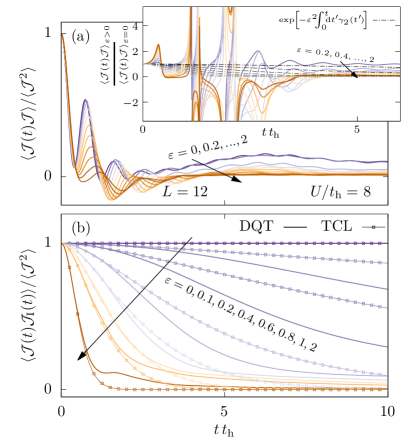
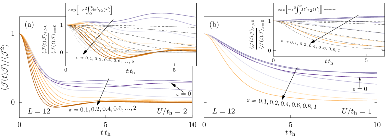
Since we have focused in the main text on a strongly interacting reference system ${\cal H}_{0}={\cal H}(U/t_{\mathrm{h}}\gg 1,U^{\prime}=0)$ with a single on-site interaction strength $U/t_{\mathrm{h}}=16$, we redo the calculation in Fig. 2 for another value of $U$. As shown in Fig. 3, the overall picture remains the same for $U/t_{\mathrm{h}}=8$. Therefore, our numerical illustration is not fine-tuned with respect to $U$. Additionally, Fig. 4 shows similar data as Fig. 3(a) but for small interaction strengths $U/t_{\mathrm{h}}=2$ and $U/t_{\mathrm{h}}=1$. Naturally, with decreasing interaction strength $U$, we start to approach the noninteracting limit where $\cal{J}$ is conserved and the oscillations in the reference dynamics disappear. However, while the ratio $\langle{\cal J}(t){\cal J}\rangle_{\varepsilon>0}/\langle{\cal J}(t){\cal J}\rangle_{\varepsilon=0}$ assumes a more well-behaved shape, the relation between perturbed and unperturbed dynamics remains hardly reconcilable with exponential damping for $U/t_{\mathrm{h}}=2$.

Appendix B Finite-size scaling

B.1 Interacting reference system

Figure 5: Second-order (a) kernel $k_{2}(t)$ and (b) damping $\gamma_{2}(t)$, as both given in Eq. (9) of the main text, for the interacting $\mathcal{H}_{0}=\mathcal{H}(U/t_{\text{h}}=16,U^{\prime}=0)$. Numerical results from DQT are shown for various chain lengths $L\leq 15$.

Figure 6: Time dependence of the current autocorrelation function $\langle{\cal J}(t){\cal J}\rangle$ in the strongly interacting system ${\cal H}(U/t_{\mathrm{h}}=16,U^{\prime}=0)$, as obtained from DQT for different system sizes $L\leq 15$. For such $L$, data are converged up to times $t\,t_{\mathrm{h}}\sim 4$. Similar data can be found in Jin et al. (2015).

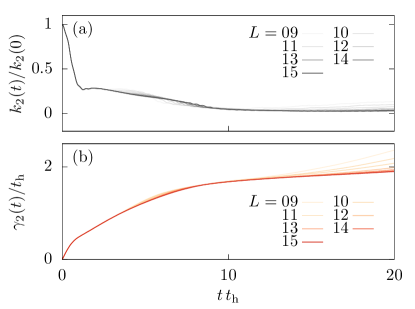
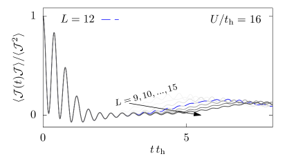
In the main text, we have mentioned in the context of Fig. 2 that the corresponding kernel $k_{2}(t)$ and the rate $\gamma_{2}(t)$ are converged with respect to system size for the relevant time scales. To support this, we depict in Fig. 5 the numerical results for $k_{2}(t)$ and $\gamma_{2}(t)$ for different system sizes $L\leq 15$. We have also mentioned that finite-size effects for the strongly interacting case $U/t_{\mathrm{h}}=16$ in Fig. 2 occur for times $t\,t_{\mathrm{h}}\sim 4$. Since we have shown curves for a single system size $L=12$ there, we now illustrate in Fig. 6 these finite-size effects explicitly by depicting curves for different system sizes $L\leq 15$. We do so for ${\cal H}(U/t_{\mathrm{h}}=16,U^{\prime}=0)$, which enters as ${\cal H}_{0}$ the interaction picture for all perturbations $U^{\prime}/t_{\mathrm{h}}=\varepsilon>0$.

B.2 Noninteracting reference system

Figure 7: Time dependence of the current autocorrelation function $\langle\mathcal{J}(t)\mathcal{J}\rangle$ in the noninteracting system $\mathcal{H}_{0}=\mathcal{H}(U=U^{\prime}=0)$, which is perturbed by interactions $U/t_{\mathrm{h}}=U^{\prime}/t_{\mathrm{h}}=\varepsilon$ for two exemplary strengths (a) $\varepsilon=0.2$ and (b) $\varepsilon=0.6$. Numerical results from DQT are shown for different system sizes $L=9,...,16$ and compared to the lowest-order prediction of the TCL projection-operator technique in Eq. (10) of the main text. For the TCL curves, different rates $\gamma_{2}(t)$ corresponding to finite system sizes $L=15$ (TCL15), $L=16$ (TCL16), as well as its estimate for $L\to\infty$ (TCL$\infty$) are used [cf. Fig. 1(c) of the main text]. Additionally, NLCE data is shown for expansion orders $c_{\mathrm{max}}\leq 15$.

In the discussion of Fig. 1 in the main text, we have mentioned that small differences between direct DQT calculations and lowest-order TCL predictions of the current autocorrelation function $\langle\mathcal{J}(t)\mathcal{J}\rangle$ might in part be related to residual finite-size effects. To support this, we depict similar data for different system sizes and for two exemplary perturbation strengths $\varepsilon=0.2$ and $\varepsilon=0.6$ in Fig. 7. Numerical results from DQT for different system sizes $L\leq 16$ are shown and compared to the lowest-order prediction of the TCL projection operator technique in Eq. (10) of the main text. Here, we show three different curves (labeled as TCL15, TCL16, and TCL$\infty$), corresponding to the rate $\gamma_{2}(t)$ obtained for the two largest numerically accessible chain lengths $L=15,16$ as well as its estimate for the thermodynamic limit $L\to\infty$, featuring a constant plateau for $t\,t_{\mathrm{h}}\gtrsim 4$ [see Fig. 1(c) of the main text]. For $\varepsilon=0.2$ [Fig. 7(a)], the DQT curves for the largest system sizes are converged up to times $t\,t_{\mathrm{h}}\sim 5$ and coincide with all three TCL curves. For later times, both the DQT and the TCL results show mild finite-size effects, whereby the TCL$\infty$ prediction appears to agree best with the scaling behavior of the DQT data. For $\varepsilon=0.6$ [Fig. 7(b)], a very similar behavior is found in the comparison of the DQT and the TCL curves.

Complementary to the DQT and the TCL data, Fig. 7 also shows numerical results for $\langle\mathcal{J}(t)\mathcal{J}\rangle$ in the thermodynamic limit $L\to\infty$ as obtained by means of a numerical linked-cluster expansion (NLCE) (see, e.g., Refs. Rigol et al. (2006); Richter and Steinigeweg (2019) and below) for different expansion orders $c_{\mathrm{max}}\leq 15$. The NLCE results agree with the DQT and the TCL data at times $t\,t_{\mathrm{h}}\lesssim 5$ for both $\varepsilon=0.2$ and $\varepsilon=0.6$. Beyond times $t\,t_{\mathrm{h}}\sim 5$, the NLCE does not add much to the information on the thermodynamic limit for $\varepsilon=0.2$. However, for $\varepsilon=0.6$, the NLCE curves are converged just long enough to indicate that the TCL$\infty$ prediction is most suitable to describe $\langle\mathcal{J}(t)\mathcal{J}\rangle$ in the thermodynamic limit.

B.2.1 NLCE in a nutshell

In the framework of NLCE, the per-site value of the current autocorrelation function on an infinite chain can be expanded in terms of its respective weights $W_{c}$ on all linked (sub-)clusters (i.e., open-boundary chains of different lengths $c$),

$$\langle\mathcal{J}(t)\mathcal{J}\rangle/L=\sum_{c}W_{c}(t)\ .$$ (15)

For numerical calculations, the sum in Eq. (15) naturally has to be truncated to the maximum accessible cluster size $c_{\mathrm{max}}$. This, together with the inclusion-exclusion principle for the calculation of each weight, $W_{c}(t)=\langle\mathcal{J}(t)\mathcal{J}\rangle^{(c)}-\sum_{s\subset c}W_{s}(t)$, results in the very simple expression approximating Eq. (15),

$$\sum_{c}^{c_{\mathrm{max}}}W_{c}(t)=\langle\mathcal{J}(t)\mathcal{J}\rangle^{(c_{\mathrm{max}})}-\langle\mathcal{J}(t)\mathcal{J}\rangle^{(c_{\mathrm{max}}-1)}\ ,$$ (16)

which is reliable up to a certain maximum time, increasing with the maximum cluster size $c_{\mathrm{max}}$. The $\langle\mathcal{J}(t)\mathcal{J}\rangle^{(c)}$ (evaluated on open-boundary chains of length $c$) are again obtained with DQT and additionally averaged over multiple random states in order to counteract the sensitivity of the difference in Eq. (16) to small statistical errors.

Appendix C Relation to correlation functions

To see that $\langle{\cal J}{\cal P}\rho_{\mathrm{I}}(t)\rangle\propto\langle{\cal J}(t){\cal J}_{\mathrm{I}}(t)\rangle$, we first insert the definition of the projection superoperator $\cal P$ in $\langle{\cal J}{\cal P}\rho_{\mathrm{I}}(t)\rangle$, which yields

$$\langle{\cal J}{\cal P}\rho_{\mathrm{I}}(t)\rangle=\langle{\cal J}\Big{(}\frac{1}{D}+\frac{\langle{\cal J}\rho_{\mathrm{I}}(t)\rangle}{\langle{\cal J}^{2}\rangle}\,{\cal J}\Big{)}\rangle\,.$$ (17)

Since $\langle{\cal J}\rangle=0$, performing the outer angles leads to

$$\langle{\cal J}{\cal P}\rho_{\mathrm{I}}(t)\rangle=\langle{\cal J}\rho_{\mathrm{I}}(t)\rangle\,.$$ (18)

We then insert the initial condition $\rho(0)\propto 1+b\cal{J}$ and use the time dependence of a density matrix in the interaction picture, $\rho_{\mathrm{I}}(t)=e^{i{\cal H}_{0}t}\,e^{-i{\cal H}t}\,\rho(0)\,e^{i{\cal H}t}\,e^{-i{\cal H}_{0}t}$, to obtain

$$\langle{\cal J}{\cal P}\rho_{\mathrm{I}}(t)\rangle\propto\langle{\cal J}e^{i{\cal H}_{0}t}\,e^{-i{\cal H}t}\,(1+b{\cal J})\,e^{i{\cal H}t}\,e^{-i{\cal H}_{0}t}\rangle\,.$$ (19)

Using $\langle{\cal J}\rangle=0$ again, we thus get

$$\langle{\cal J}{\cal P}\rho_{\mathrm{I}}(t)\rangle\propto\langle{\cal J}e^{i{\cal H}_{0}t}\,e^{-i{\cal H}t}\,{\cal J}\,e^{i{\cal H}t}\,e^{-i{\cal H}_{0}t}\rangle\,,$$ (20)

which, after a cyclic permutation, reads

$$\langle{\cal J}{\cal P}\rho_{\mathrm{I}}(t)\rangle\propto\langle e^{-i{\cal H}t}\,{\cal J}e^{i{\cal H}t}\,e^{-i{\cal H}_{0}t}\,{\cal J}\,e^{i{\cal H}_{0}t}\rangle\,.$$ (21)

Denoting by ${\cal J}(t)=e^{i{\cal H}t}\,{\cal J}\,e^{-i{\cal H}t}$ and ${\cal J}_{\mathrm{I}}(t)=e^{i{\cal H}_{0}t}\,{\cal J}\,e^{-i{\cal H}_{0}t}$ the time evolution of an operator in the Heisenberg and interaction picture, respectively, we can write

$$\langle{\cal J}{\cal P}\rho_{\mathrm{I}}(t)\rangle\propto\langle{\cal J}(-t){\cal J}_{\mathrm{I}}(-t)\rangle\,.$$ (22)

Due to ${\cal J}^{\dagger}={\cal J}$, we can replace $t\to-t$ and end up with

$$\langle{\cal J}{\cal P}\rho_{\mathrm{I}}(t)\rangle\propto\langle{\cal J}(t){\cal J}_{\mathrm{I}}(t)\rangle\,.$$ (23)

Appendix D Conductivity

Figure 8: Frequency dependence of the conductivity $\sigma(\omega)$, as obtained by the Fourier transform (24) of the current autocorrelation functions shown in Fig. 2(a) of the main text.

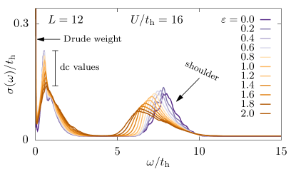
In Fig. 8, we show the frequency-dependent conductivity in the strongly interacting system ${\cal H}(U/t_{\mathrm{h}}=16,U^{\prime}=0)$, perturbed by interactions $U^{\prime}/t_{\mathrm{h}}=\varepsilon$. This conductivity is obtained by the Fourier transform of the current autocorrelation functions depicted in Fig. 2(a) of the main text,

$$\sigma(\omega)=\int^{t_{\mathrm{max}}}_{-t_{\mathrm{max}}}\mathrm{d}t\ \mathrm{e}^{-i\omega t}\,\frac{\langle\mathcal{J}(t)\mathcal{J}\rangle}{L}\ ,$$ (24)

with a cutoff time $t_{\mathrm{max}}\,t_{\mathrm{h}}=100$. The overall shape of the conductivity is incompatible with a simple Lorentzian form, while the freestanding shoulder shifts from higher to lower $\omega$ as the perturbation strength increases, attesting to the shift in the frequencies observed in the oscillatory behavior of the corresponding current autocorrelation functions. In addition, the spectral weight at small $\omega$ provides a rough estimate for the value of the dc conductivity $\sigma_{\mathrm{d}c}$, which clearly does not scale as $\sigma_{\text{dc}}\propto 1/\varepsilon^{2}$. For the detailed extraction of $\sigma_{\text{dc}}$, see Ref. Bertini et al. (2021).

References

- D’Alessio et al. (2016) L. D’Alessio, Y. Kafri, A. Polkovnikov, and M. Rigol, Adv. Phys. 65, 239 (2016).
- Borgonovi et al. (2016) F. Borgonovi, F. Izrailev, L. F. Santos, and V. Zelevinsky, Phys. Rep. 626, 1 (2016).
- Gogolin and Eisert (2016) C. Gogolin and J. Eisert, Rep. Prog. Phys. 79, 056001 (2016).
- Paeckel et al. (2019) S. Paeckel, T. Köhler, A. Swoboda, S. R. Manmana, U. Schollwöck, and C. Hubig, Ann. Phys. (NY) 411, 167998 (2019).
- Dziarmaga (2010) J. Dziarmaga, Adv. Phys. 59, 1063 (2010).
- Polkovnikov et al. (2011) A. Polkovnikov, K. Sengupta, A. Silva, and M. Vengalattore, Rev. Mod. Phys. 83, 863 (2011).
- Erne et al. (2018) S. Erne, R. Bücker, T. Gasenzer, J. Berges, and J. Schmiedmayer, Nature 563, 225 (2018).
- Prüfer et al. (2018) M. Prüfer, P. Kunkel, H. Strobel, S. Lannig, D. Linnemann, C.-M. Schmied, J. Berges, T. Gasenzer, and M. K. Oberthaler, Nature 563, 217 (2018).
- Reimann et al. (2020) P. Reimann, B. N. Balz, J. Richter, and R. Steinigeweg, Phys. Rev. B 101, 094302 (2020).
- Alhambra et al. (2020) Á. M. Alhambra, J. Riddell, and L. P. García-Pintos, Phys. Rev. Lett. 124, 110605 (2020).
- Brody et al. (1981) T. A. Brody, J. Flores, J. B. French, P. A. Mello, A. Pandey, and S. S. M. Wong, Rev. Mod. Phys. 53, 385 (1981).
- Deutsch (1991) J. M. Deutsch, Phys. Rev. A 43, 2046 (1991).
- Srednicki (1994) M. Srednicki, Phys. Rev. E 50, 888 (1994).
- Rigol et al. (2008) M. Rigol, V. Dunjko, and M. Olshanii, Nature 452, 854 (2008).
- Khaymovich et al. (2019) I. M. Khaymovich, M. Haque, and P. A. McClarty, Phys. Rev. Lett. 122, 070601 (2019).
- Richter et al. (2020a) J. Richter, A. Dymarsky, R. Steinigeweg, and J. Gemmer, Phys. Rev. E 102, 042127 (2020a).
- Schönle et al. (2021) C. Schönle, D. Jansen, F. Heidrich-Meisner, and L. Vidmar, Phys. Rev. B 103, 235137 (2021).
- Brenes et al. (2021) M. Brenes, S. Pappalardi, M. T. Mitchison, J. Goold, and A. Silva, Phys. Rev. E 104, 034120 (2021).
- von Keyserlingk et al. (2018) C. W. von Keyserlingk, T. Rakovszky, F. Pollmann, and S. L. Sondhi, Phys. Rev. X 8, 021013 (2018).
- Nahum et al. (2018) A. Nahum, S. Vijay, and J. Haah, Phys. Rev. X 8, 021014 (2018).
- Khemani et al. (2018) V. Khemani, A. Vishwanath, and D. A. Huse, Phys. Rev. X 8, 031057 (2018).
- Knipschild and Gemmer (2018) L. Knipschild and J. Gemmer, Phys. Rev. E 98, 062103 (2018).
- Nation and Porras (2019) C. Nation and D. Porras, Phys. Rev. E 99, 052139 (2019).
- Dabelow and Reimann (2020a) L. Dabelow and P. Reimann, Phys. Rev. Lett. 124, 120602 (2020a).
- Dabelow and Reimann (2021) L. Dabelow and P. Reimann, J. Stat. Mech. 2021, 013106 (2021).
- Richter et al. (2020b) J. Richter, F. Jin, L. Knipschild, H. De Raedt, K. Michielsen, J. Gemmer, and R. Steinigeweg, Phys. Rev. E 101, 062133 (2020b).
- Berges et al. (2004) J. Berges, S. Borsányi, and C. Wetterich, Phys. Rev. Lett. 93, 142002 (2004).
- Moeckel and Kehrein (2008) M. Moeckel and S. Kehrein, Phys. Rev. Lett. 100, 175702 (2008).
- Bertini et al. (2015) B. Bertini, F. H. L. Essler, S. Groha, and N. J. Robinson, Phys. Rev. Lett. 115, 180601 (2015).
- Mori et al. (2018) T. Mori, T. N. Ikeda, E. Kaminishi, and M. Ueda, J. Phys. B 51, 112001 (2018).
- Reimann and Dabelow (2019) P. Reimann and L. Dabelow, Phys. Rev. Lett. 122, 080603 (2019).
- Mallayya et al. (2019) K. Mallayya, M. Rigol, and W. De Roeck, Phys. Rev. X 9, 021027 (2019).
- Schmitt and Kehrein (2018) M. Schmitt and S. Kehrein, Phys. Rev. B 98, 180301(R) (2018).
- Dabelow and Reimann (2020b) L. Dabelow and P. Reimann, Phys. Rev. Research 2, 023216 (2020b).
- Preskill (2018) J. Preskill, Quantum 2, 79 (2018).
- Arute et al. (2019) F. Arute et al., Nature 574, 505 (2019).
- Genway et al. (2013) S. Genway, A. F. Ho, and D. K. K. Lee, Phys. Rev. Lett. 111, 130408 (2013).
- Werner et al. (2020) M. A. Werner, C. P. Moca, Ö. Legeza, and G. Zaránd, Phys. Rev. B 102, 155108 (2020).
- Popescu et al. (2006) S. Popescu, A. J. Short, and A. Winter, Nat. Phys. 2, 754 (2006).
- Goldstein et al. (2006) S. Goldstein, J. L. Lebowitz, R. Tumulka, and N. Zanghì, Phys. Rev. Lett. 96, 050403 (2006).
- Bartsch et al. (2008) C. Bartsch, R. Steinigeweg, and J. Gemmer, Phys. Rev. E 77, 011119 (2008).
- Reimann (2018) P. Reimann, Phys. Rev. E 97, 062129 (2018).
- Breuer and Petruccione (2007) H.-P. Breuer and F. Petruccione, The Theory of Open Quantum Systems (Oxford University Press, 2007).
- Zotos and Prelovšek (2004) X. Zotos and P. Prelovšek, in Strong interactions in low dimensions (Springer Netherlands, Dordrecht, 2004) Chap. 11, pp. 347–382.
- Bertini et al. (2021) B. Bertini, F. Heidrich-Meisner, C. Karrasch, T. Prosen, R. Steinigeweg, and M. Žnidarič, Rev. Mod. Phys. 93, 025003 (2021).
- Bulchandani et al. (2021) V. B. Bulchandani, S. Gopalakrishnan, and E. Ilievski, J. Stat. Mech. 2021, 084001 (2021).
- Essler et al. (2005) F. H. L. Essler, H. Frahm, F. Göhmann, A. Klümper, and V. E. Korepin, The One-Dimensional Hubbard Model (Cambridge University Press, 2005).
- (48) A canonical density matrix with a sufficiently small inverse temperature can be expanded as Kubo et al. (1991); Brenig (1989).
- Kubo et al. (1991) R. Kubo, M. Toda, and N. Hashitsume, Statistical Physics II, 2nd ed., Springer Series in Solid-State Sciences, Vol. 31 (Springer Berlin Heidelberg, 1991).
- Brenig (1989) W. Brenig, Statistical Theory of Heat (Springer Berlin Heidelberg, 1989).
- Chaturvedi and Shibata (1979) S. Chaturvedi and F. Shibata, Z. Phys. B 35, 297 (1979).
- Steinigeweg (2011) R. Steinigeweg, Phys. Rev. E 84, 011136 (2011).
- Bartsch and Gemmer (2009) C. Bartsch and J. Gemmer, Phys. Rev. Lett. 102, 110403 (2009).
- Jin et al. (2021) F. Jin, D. Willsch, M. Willsch, H. Lagemann, K. Michielsen, and H. De Raedt, J. Phys. Soc. Jpn. 90, 012001 (2021).
- Heitmann et al. (2020) T. Heitmann, J. Richter, D. Schubert, and R. Steinigeweg, Z. Naturforsch. A 75, 421 (2020).
- Iitaka and Ebisuzaki (2003) T. Iitaka and T. Ebisuzaki, Phys. Rev. Lett. 90, 047203 (2003).
- Elsayed and Fine (2013) T. A. Elsayed and B. V. Fine, Phys. Rev. Lett. 110, 070404 (2013).
- Prosen and Žnidarič (2002) T. Prosen and M. Žnidarič, J. Phys. A 35, 1455 (2002).
- Karrasch et al. (2014a) C. Karrasch, D. M. Kennes, and J. E. Moore, Phys. Rev. B 90, 155104 (2014a).
- Jin et al. (2015) F. Jin, R. Steinigeweg, F. Heidrich-Meisner, K. Michielsen, and H. De Raedt, Phys. Rev. B 92, 205103 (2015).
- Zotos (2004) X. Zotos, Phys. Rev. Lett. 92, 067202 (2004).
- Jung et al. (2006) P. Jung, R. W. Helmes, and A. Rosch, Phys. Rev. Lett. 96, 067202 (2006).
- Steinigeweg et al. (2016) R. Steinigeweg, J. Herbrych, X. Zotos, and W. Brenig, Phys. Rev. Lett. 116, 017202 (2016).
- Karrasch et al. (2014b) C. Karrasch, J. E. Moore, and F. Heidrich-Meisner, Phys. Rev. B 89, 075139 (2014b).
- Karrasch et al. (2015) C. Karrasch, D. M. Kennes, and F. Heidrich-Meisner, Phys. Rev. B 91, 115130 (2015).
- Steinigeweg et al. (2014) R. Steinigeweg, F. Heidrich-Meisner, J. Gemmer, K. Michielsen, and H. De Raedt, Phys. Rev. B 90, 094417 (2014).
- Rigol et al. (2006) M. Rigol, T. Bryant, and R. R. P. Singh, Phys. Rev. Lett. 97, 187202 (2006).
- Richter and Steinigeweg (2019) J. Richter and R. Steinigeweg, Phys. Rev. B 99, 094419 (2019).