A primal-dual flow for affine constrained convex optimization

Abstract

We introduce a novel primal-dual flow for affine constrained convex optimization problems. As a modification of the standard saddle-point system, our primal-dual flow is proved to possess the exponential decay property, in terms of a tailored Lyapunov function. Then two primal-dual methods are obtained from numerical discretizations of the continuous model, and global nonergodic linear convergence rate is established via a discrete Lyapunov function. Instead of solving the subproblem of the primal variable, we apply the semi-smooth Newton iteration to the subproblem with respect to the multiplier, provided that there are some additional properties such as semi-smoothness and sparsity. Especially, numerical tests on the linearly constrained $l_{1}$-$l_{2}$ minimization and the total-variation based image denoising model have been provided.

Keywords: convex optimization, linear constraint, dynamical system, Lyapunov function, exponential decay, discretization, nonergodic linear rate, primal-dual algorithm, semi-smooth Newton method, $l_{1}$-$l_{2}$ minimization, total-variation model

1 Introduction

We are interested in the linearly constrained minimization problem

$$\mathop{\min}_{x\in\,{\mathbb{R}}^{n}}f(x)\quad{\rm s.t.~{}}Ax=b,$$ (1)

where $(A,b)\in\,{\mathbb{R}}^{m\times n}\times\,{\mathbb{R}}^{m}$ and $f:\,{\mathbb{R}}^{n}\to\,{\mathbb{R}}\cup\{+\infty\}$ is proper, closed and convex. Let $\Omega:=\,{\mathbb{R}}^{n}\times\,{\mathbb{R}}^{m}$ and introduce the Lagrangian

$$\mathcal{L}(x,\lambda):=f(x)+\left\langle{\lambda,Ax-b}\right\rangle\quad\forall\,(x,\lambda)\in\Omega,$$ (2)

where $\left\langle{\cdot,\cdot}\right\rangle$ denotes the standard $l^{2}$-inner product, with $\left\lVert{\cdot}\right\rVert=\sqrt{\left\langle{\cdot,\cdot}\right\rangle}$ being the Euclidean norm. Assume $(x^{*},\lambda^{*})$ is a saddle-point of $\mathcal{L}(x,\lambda)$, which means

$$\mathcal{L}(x^{*},\lambda)\leqslant\mathcal{L}(x^{*},\lambda^{*})\leqslant\mathcal{L}(x,\lambda^{*})\quad\forall\,(x,\lambda)\in\Omega,$$

and denote by $\Omega^{*}$ the set of all saddle-points. Any $(x^{*},\lambda^{*})\in\Omega^{*}$ satisfies the Karush–Kuhn–Tucker (KKT) system

$$\left\{\begin{aligned} {}&0=\nabla_{\lambda}\mathcal{L}(x^{*},\lambda^{*})=Ax^{*}-b,\\ {}&0\in\partial_{x}\mathcal{L}(x^{*},\lambda^{*})=\partial f(x^{*})+A^{\top}\lambda^{*},\end{aligned}\right.$$ (3)

where $\partial f(x^{*})$ is the subdifferential of $f$ at $x^{*}$.

For the standard model problem 1, there are a large body of primal-dual type algorithms that achieve the fast (ergodic) sublinear rate $\mathcal{O}(1/k^{2})$ with strongly convex condition; see Section 1.2 for a brief review. Meanwhile, some existing works also focus on the asymptotic convergence from the continuous-time point of view, i.e., the saddle-point dynamical system [23, 33]

$$\left\{\begin{aligned} {}&\lambda^{\prime}={}\nabla_{\lambda}\mathcal{L}(x,\lambda),\\ {}&x^{\prime}=-\nabla_{x}\mathcal{L}(x,\lambda).\end{aligned}\right.$$ (4)

In this work, we shall modify the conventional model 4 and introduce a novel primal-dual flow system which possesses exponential decay property. New primal-dual algorithms shall be obtained from proper time discretizations and nonergodic linear convergence rate will be proved via the tool of Lyapunov function.

To move on, let us make some conventions. We say a function $g:\,{\mathbb{R}}^{n}\to\,{\mathbb{R}}$ is $L$-smooth if it has $L$-Lipschitz continuous gradient:

$$\left\lVert{\nabla g(x)-\nabla g(y)}\right\rVert\leqslant L\left\lVert{x-y}\right\rVert\quad\forall\,x,y\in\,{\mathbb{R}}^{n}.$$

For a properly closed convex function $g:\,{\mathbb{R}}^{n}\to\,{\mathbb{R}}\cup\{+\infty\}$, it is called $\mu$-convex if there exists $\mu\geqslant 0$ such that

$$g(x)+\left\langle{p,y-x}\right\rangle+\frac{\mu}{2}\left\lVert{y-x}\right\rVert^{2}\leqslant g(y),$$

for all $p\in\partial g(x)$. The proximal mapping ${\bf prox}_{\theta g}:\,{\mathbb{R}}^{n}\to\,{\mathbb{R}}^{n}$ of $g$ with $\theta>0$ is defined by

$${\bf prox}_{\theta g}(x):=({\rm Id}+\theta\partial g)^{-1}(x)=\mathop{{\mathop{{\rm argmin}}\,}}\limits_{y\in\,{\mathbb{R}}^{n}}\left\{g(y)+\frac{1}{2\theta}\left\lVert{y-x}\right\rVert^{2}\right\}\quad\forall\,x\in\,{\mathbb{R}}^{n},$$

where $\,{\rm Id}$ denotes the identity operator. Clearly, if $f$ is $\mu$-convex, then according to 2, we claim that $\mathcal{L}(\cdot,\lambda)$ is also $\mu$-convex and

$$\mathcal{L}(x,\lambda)+\left\langle{p+A^{\top}\lambda,y-x}\right\rangle+\frac{\mu}{2}\left\lVert{y-x}\right\rVert^{2}\leqslant\mathcal{L}(y,\lambda),\quad p\in\partial f(x).$$ (5)

1.1 Main results

Following the time rescaling technique and the tool of Lyapunov function from [58, 19], for smooth and $\mu$-convex objective $f$, we propose a primal-dual flow

$$\left\{\begin{aligned} {}&\gamma x^{\prime}=-\nabla_{x}\mathcal{L}(x,\lambda),\\ {}&\beta\lambda^{\prime}={}\nabla_{\lambda}\mathcal{L}(x+x^{\prime},\lambda),\end{aligned}\right.$$ (6)

where $\gamma$ and $\beta$ are two nonnegative scaling factors that are governed by $\gamma^{\prime}={}\mu-\gamma$ and $\beta^{\prime}=-\beta$, respectively. Compared with the classical one 4, our new model 6 has two novelties: (i) it introduces two built-in time rescaling factors that unify the analysis for $\mu\geqslant 0$; (ii) the term $\nabla_{\lambda}\mathcal{L}(x+x^{\prime},\lambda)$ (instead of the standard one $\nabla_{\lambda}\mathcal{L}(x,\lambda)$) brings stability and reduces the oscillation; see Section 2.3 for an illustrative equilibrium analysis. Besides, the extra term $x^{\prime}$ in $\nabla_{\lambda}\mathcal{L}(x+x^{\prime},\lambda)$ has subtle connection with the over-relaxation $x_{k+1}+\theta(x_{k+1}-x_{k})$ introduced in the primal-dual hybrid gradient (PDHG) method [16]; see Appendix A for a more reasonably intrinsic explanation.

We then equip the dynamical system 6 with a tailored Lyapunov function

$$\mathcal{E}(t):=\mathcal{L}(x(t),\lambda^{*})-\mathcal{L}(x^{*},\lambda(t))+\frac{\gamma(t)}{2}\left\lVert{x(t)-x^{*}}\right\rVert^{2}+\frac{\beta(t)}{2}\left\lVert{\lambda(t)-\lambda^{*}}\right\rVert^{2},\quad\,t\geqslant 0,$$

which possesses the exponential decay (see Theorem 2.1)

$$\frac{\,{\rm d}}{\,{\rm d}t}\mathcal{E}(t)\leqslant-\mathcal{E}(t)\quad\Longrightarrow\quad\mathcal{E}(t)\leqslant e^{-t}\mathcal{E}(0),\quad t\geqslant 0.$$ (7)

From 7 we have $\mathcal{L}(x(t),\lambda^{*})-\mathcal{L}(x^{*},\lambda(t))\leqslant e^{-t}\mathcal{E}(0)$, and we can further prove $\left\lvert{f(x(t))-f(x^{*})}\right\rvert+\left\lVert{Ax(t)-b}\right\rVert\leqslant Ce^{-t}$; see 2.1.

We also consider implicit and semi-implicit discretizations for the continuous flow 6 (in general nonsmooth setting) and obtain new primal-dual algorithms, which are close to the (linearized) proximal augmented Lagrangian method but adopt automatically changing parameters. In addition, instead of solving the subproblem of the primal variable, we apply the semi-smooth Newton (SsN) iteration to the subproblem with respect to the multiplier, provided that there are some hidden structures such as semi-smoothness and sparsity. By using a unified discrete Lyapunov function

$$\mathcal{E}_{k}=\mathcal{L}(x_{k},\lambda^{*})-\mathcal{L}(x^{*},\lambda_{k})+\frac{\gamma_{k}}{2}\left\lVert{x_{k}-x^{*}}\right\rVert^{2}+\frac{\beta_{k}}{2}\left\lVert{\lambda_{k}-\lambda^{*}}\right\rVert^{2},$$

we prove the contraction property:

$$\mathcal{E}_{k+1}-\mathcal{E}_{k}\leqslant-\alpha_{k}\mathcal{E}_{k+1}\quad\text{or}\quad\mathcal{E}_{k+1}-\mathcal{E}_{k}\leqslant-\alpha_{k}\mathcal{E}_{k}\quad\forall\,k\in\mathbb{N},$$

from which we obtain nonergodic convergence rates of the objective gap $\left\lvert{f(x_{k})-f(x^{*})}\right\rvert$ and the feasibility residual $\left\lVert{Ax_{k}-b}\right\rVert$. More precisely, the implicit discretization converges with (super) linear rate for convex objective $f$ and the semi-implicit scheme possesses the rate $\mathcal{O}(\min\{L/k,(1+\mu/L)^{-k}\})$ for the composite case $f=h+g$ where $h$ is $L$-smooth and $\mu$-convex and $g$ is convex (possibly nonsmooth).

1.2 Related works

As one can add the indicator function of the constraint set to the objective and get rid of the linear constraint in (1), the proximal gradient method [7], as well as the accelerated proximal gradient method [6, 20, 58, 59], can be considered. However, they need projections onto the affine constraint set and are not suitable to handle the composite case $f=h+g$.

Therefore, prevailing algorithms are the augmented Lagrangian method (ALM) [8], the Bregman iteration [62] and their variants (linearization or acceleration) [45, 48, 82, 47, 72, 75, 76]. Another type of algorithm is the quadratic penalty method with continuation technique [49, 52]. Among those methods mentioned here, the fast rate $\mathcal{O}(1/k^{2})$ is mainly in ergodic sense for primal variable and it is rare to see global nonergodic linear rate, even with strongly convex objectives. More recently, Li, Sun and Toh [53] proposed a (super) linearly convergent semi-smooth Newton based inexact proximal ALM for linear programming. Later, this method has been extended to quadratic programming [51, 60].

For the separable case: $f(x)=f_{1}(x_{1})+f_{2}(x_{2}),\,A=(A_{1},A_{2})$, we have alternating direction method of multipliers (ADMM) [36, 35] for primal problem and operator splitting methods [29, 65, 30] for dual problem. For ADMM type methods, the sublinear rate $\mathcal{O}(1/k^{2})$ can be proved under partially strong convexity assumption [70, 78, 74, 77] and global linear rate has been established as well for strongly convex (smooth) objectives [25, 37, 26]. In addition, (local) linear convergence can be derived from the error bound condition [1, 39, 55, 84, 87]. For a special case $A_{1}=I$ or $A_{2}=I$, there are primal-dual splitting methods [17, 16, 43, 31, 64, 89, 46, 9]. Generally speaking, we have sublinear rate $\mathcal{O}(1/k^{2})$ for partially strongly convex case and linear rate for strongly convex case [18, 79, 73]. Moreover, equivalence between primal-dual splitting methods and ADMM type methods can be found in [13, 85, 61].

On the other hand, ordinary differential equation (ODE) solver approach has been revisited nowadays for investigating and developing optimization methods. For unconstrained problems, there are heavy ball model [3], asymptotically vanishing dynamical (AVD) model [71] and their extensions [2, 4, 81, 80, 54]. Besides, Luo and Chen [58] proposed the so-called Nesterov accelerated gradient flow and later generalized it to [20, 19, 57].

For linearly constrained problem 1, apart from the classical first-order saddle-point system 4, some second-order dynamics have been proposed as well. Zeng, Lei and Chen [88] generalized the AVD model and obtained the decay rate $\mathcal{O}(t^{-\mathop{\min}\{2,2\alpha/3\}})$ via a suitable Lyapunov function. He, Hu and Fang [41] extended the dynamical system in [88] to separable case. Revisiting the scaled alternating direction method of multipliers [10], Franca, Robinson and Vidal [34] derived a continuous model which is also related to the AVD model and proved the decay rate $\mathcal{O}(1/t^{2})$. Yet, none of Zeng et al. [88], He et al. [41] and Franca et al. [34] neither considered numerical discretizations for their dynamical systems nor presented new optimization algorithms for the original optimization problem. For general minimax problems, there are some works on dynamical system approach [56, 22].

Comparing with existing works, we summarize our main contributions as below:

• The continuous primal-dual flow 6 adopts built-in time rescaling factors for both convex and strongly convex cases and has exponential decay rate with respect to a proper Lyapunov function.

• A simple but illustrative equilibrium analysis shows the gain of stability that is benefit from the modification introduced in 6.

• New primal-dual algorithms with automatically changing parameters are obtained from proper time discretizations of the continuous model and the semi-smooth Newton method is considered for the subproblem with respect to the multiplier.

• Nonergodic (super) linear convergence rate of the objective gap and feasibility residual is established via the tool of discrete Lyapunov function.

The rest of this paper is organized as follows. Section 2 starts from the classical saddle-point system and introduces a new primal-dual flow. Then Sections 3 and 4 consider implicit and semi-implicit discretizations respectively and establish the (super) linear convergence rates of the resulted primal-dual algorithms. Numerical performances on the $l_{1}$-$l_{2}$ minimization and the total-variation based denoising model are presented in Section 5 and finally, some concluding remarks are given in Section 6.

2 Continuous Problems

2.1 The saddle-point system

To present the main idea clearly, let us start from the rescaled saddle-point system

$$\left\{\begin{aligned} {}&\beta\lambda^{\prime}={}\nabla_{\lambda}\mathcal{L}(x,\lambda),\\ {}&\gamma x^{\prime}=-\nabla_{x}\mathcal{L}(x,\lambda),\end{aligned}\right.$$ (8)

with the initial condition $(x(0),\lambda(0))=(x_{0},\lambda_{0})\in\Omega$, where $\gamma$ and $\beta$ are two artificial time rescaling factors and satisfy (cf. [58, 19])

$$\gamma^{\prime}=\mu-\gamma\quad\beta^{\prime}=-\beta,$$ (9)

with positive initial condition $(\gamma(0),\beta(0))=(\gamma_{0},\beta_{0})$. One can easily solve 9 to obtain

$$\gamma(t)={}\gamma_{0}e^{-t}+\mu(1-e^{-t})\quad\text{and}\quad\quad\beta(t)={}\beta_{0}e^{-t}\quad t\geqslant 0,$$ (10)

which implies $\gamma$ and $\beta$ are positive and converge exponentially to $\mu$ and $0$, respectively.

Assume $f\in C^{1}_{L}$ and define $F:\,{\mathbb{R}}_{+}\times\Omega\to\Omega$ by that

$$F(t,Z):=\begin{pmatrix}\displaystyle-\frac{1}{\gamma(t)}\nabla_{x}\mathcal{L}(x,\lambda)\\ \displaystyle\frac{1}{\beta(t)}\nabla_{\lambda}\mathcal{L}(x,\lambda)\end{pmatrix}\quad\forall\,Z=\begin{pmatrix}x\\ \lambda\end{pmatrix}\in\Omega.$$

Then 8 can be rewritten as $Z^{\prime}(t)=F(t,Z(t))$ and a direct calculation yields that for all $Z,\,Y\in\Omega$ and $0\leqslant s\leqslant t$,

$$\left\lVert{F(t,Z)-F(s,Y)}\right\rVert\leqslant C_{0}(L+\left\lVert{A}\right\rVert)\left(\left\lvert{t-s}\right\rvert\left\lVert{Z-Z^{*}}\right\rVert+\left\lVert{Z-Y}\right\rVert\right)e^{t},$$

where $Z^{*}=(x^{*},\lambda^{*})\in\Omega^{*}$ and the bounded positive constant $C_{0}$ depends only on $\gamma_{0},\beta_{0}$ and $\mu$. This means $F$ is locally Lipschitz continuous and according to [40, Proposition 6.2.1] and [11, Corollary A.2], the first-order dynamical system 8 exists a unique solution $Z=(x,\lambda)\in C^{1}(\,{\mathbb{R}}_{+};\Omega)$.

Let $\bm{V}:=\Omega\times\,{\mathbb{R}}_{+}\times\,{\mathbb{R}}_{+}$ and for any $X=(x,\lambda,\gamma,\beta)\in\bm{V}$, introduce a Lyapunov function

$$\mathcal{E}(X):=\mathcal{L}(x,\lambda^{*})-\mathcal{L}(x^{*},\lambda)+\frac{\gamma}{2}\left\lVert{x-x^{*}}\right\rVert^{2}+\frac{\beta}{2}\left\lVert{\lambda-\lambda^{*}}\right\rVert^{2}.$$ (11)

Our goal is to establish the exponential decay property of (11) along with the solution trajectory $X:\,{\mathbb{R}}_{+}\to\bm{V}$. Below, we present a lemma which violates our goal but heuristically motivates us to the right way.

Lemma 2.1.

Assume $f$ is $L$-smooth and $\mu$-convex with $\mu\geqslant 0$ and let $X=(x,\lambda,\gamma,\beta):\,{\mathbb{R}}_{+}\to\bm{V}$ be the unique solution to 8 and 9, then

$$\frac{\rm d}{{\rm d}t}\mathcal{E}(X)\leqslant-\mathcal{E}(X)-\gamma\left\lVert{x^{\prime}}\right\rVert^{2}-\left\langle{Ax^{\prime},\lambda-\lambda^{*}}\right\rangle.$$ (12)

Proof.

As discussed above, $(x,\lambda)\in C^{1}(\,{\mathbb{R}}_{+};\Omega)$ exists uniquely and by 8, a direct computation gives

$$\begin{split}\frac{\rm d}{{\rm d}t}\mathcal{E}(X)={}&\left\langle{\nabla_{x}\mathcal{E}(X),x^{\prime}}\right\rangle+\left\langle{\nabla_{\lambda}\mathcal{E}(X),\lambda^{\prime}}\right\rangle+\left\langle{\nabla_{\gamma}\mathcal{E}(X),\gamma^{\prime}}\right\rangle+\left\langle{\nabla_{\beta}\mathcal{E}(X),\beta^{\prime}}\right\rangle\\ ={}&\underbrace{-\frac{1}{\gamma}\left\langle{\nabla_{x}\mathcal{L}(x,\lambda),\nabla_{x}\mathcal{L}(x,\lambda^{*})}\right\rangle}_{I_{1}}+\underbrace{\left\langle{\nabla_{\lambda}\mathcal{L}(x,\lambda),\lambda-\lambda^{*}}\right\rangle-\left\langle{\nabla_{x}\mathcal{L}(x,\lambda),x-x^{*}}\right\rangle}_{I_{2}}\\ {}&\qquad\underbrace{-\frac{\beta}{2}\left\lVert{\lambda-\lambda^{*}}\right\rVert^{2}+\frac{\mu-\gamma}{2}\left\lVert{x-x^{*}}\right\rVert^{2}}_{I_{3}}\\ :={}&I_{1}+I_{2}+I_{3}.\end{split}$$

We split $\nabla_{x}\mathcal{L}(x,\lambda^{*})=\nabla_{x}\mathcal{L}(x,\lambda)-A^{\top}(\lambda-\lambda^{*})$ and use the relation $\gamma x^{\prime}=-\nabla_{x}\mathcal{L}(x,\lambda)$ to get

$$\begin{split}I_{1}=&-\frac{1}{\gamma}\left\langle{\nabla_{x}\mathcal{L}(x,\lambda),\nabla_{x}\mathcal{L}(x,\lambda)-A^{\top}(\lambda-\lambda^{*})}\right\rangle=-\gamma\left\lVert{x^{\prime}}\right\rVert^{2}-\left\langle{Ax^{\prime},\lambda-\lambda^{*}}\right\rangle.\end{split}$$ (13)

Also, we reformulate $I_{2}$ as follows

$$\small\begin{split}I_{2}={}&\left\langle{\nabla_{\lambda}\mathcal{L}(x,\lambda),\lambda-\lambda^{*}}\right\rangle-\left\langle{Ax-Ax^{*},\lambda-\lambda^{*}}\right\rangle-\left\langle{\nabla_{x}\mathcal{L}(x,\lambda^{*}),x-x^{*}}\right\rangle=-\left\langle{\nabla_{x}\mathcal{L}(x,\lambda^{*}),x-x^{*}}\right\rangle,\end{split}$$ (14)

where we have used the optimality condition $Ax^{*}=b$. Since $f$ is $\mu$-convex, we know that $\mathcal{L}(\cdot,\lambda^{*})$ is also $\mu$-convex and it follows from 5 that

$$\begin{split}I_{2}\leqslant{}&\mathcal{L}(x,\lambda^{*})-\mathcal{L}(x^{*},\lambda^{*})-\frac{\mu}{2}\left\lVert{x-x^{*}}\right\rVert^{2}={}\mathcal{L}(x,\lambda^{*})-\mathcal{L}(x^{*},\lambda)-\frac{\mu}{2}\left\lVert{x-x^{*}}\right\rVert^{2}.\end{split}$$

Here, recall the fact that $\mathcal{L}(x^{*},\cdot)$ is a constant. Hence, collecting $I_{3}$, 13 and 14 proves (12). ∎

To obtain $\mathcal{E}^{\prime}(X)\leqslant-\mathcal{E}(X)$ from (12), we shall prove $-\gamma\left\lVert{x^{\prime}}\right\rVert^{2}-\left\langle{Ax^{\prime},\lambda-\lambda^{*}}\right\rangle\leqslant 0$. In stead of twisting on the existence of this, in the next section, we resort to introducing a subtle modification that cancels exactly the cross term $\left\langle{Ax^{\prime},\lambda-\lambda^{*}}\right\rangle$ in (12) and finally leads to the desired estimate.

2.2 A new primal-dual flow

Although (12) fails to give the desired result, it suggests a simple remedy: replacing $\nabla_{\lambda}\mathcal{L}(x,\lambda)$ by $\nabla_{\lambda}\mathcal{L}(x+x^{\prime},\lambda)$. Then the first part $I_{1}$ (cf. (13)) brings one more term $\left\langle{Ax^{\prime},\lambda-\lambda^{*}}\right\rangle$ which offsets exactly the last term in (12) while both $I_{2}$ and $I_{3}$ keep unchanged.

Namely, we leave the parameter system 9 invariant but modify 8 properly to obtain a novel primal-dual flow

$$\gamma x^{\prime}=-\nabla_{x}\mathcal{L}(x,\lambda),$$ (15a)

$$\beta\lambda^{\prime}={}\nabla_{\lambda}\mathcal{L}(x+x^{\prime},\lambda).$$ (15b)

Similar with 8, we claim that 15b admits a unique classical solution $(x,\lambda)\in C^{1}(\,{\mathbb{R}}_{+};\Omega)$. We also mention that the extrapolation idea $x+x^{\prime}$ in (15b) can be found previously in the second-order primal-dual ODE proposed by [88]. In the sequel, we shall complete the exponential decay of the Lyapunov function (11) and then provide an illustrative equilibrium analysis that gives a convincible explanation of the subtle modification $x+x^{\prime}$. Additionally, in Appendix A, we present an over-relaxation perspective, which perhaps shows the intrinsic connection with the PDHG method [16].

Theorem 2.1.

Assume $f$ is $L$-smooth and $\mu$-convex with $\mu\geqslant 0$ and let $X=(x,\lambda,\gamma,\beta):\,{\mathbb{R}}_{+}\to\bm{V}$ be the unique solution to 9 and 15a, then

$$\frac{\rm d}{{\rm d}t}\mathcal{E}(X)\leqslant-\mathcal{E}(X)-\gamma\left\lVert{x^{\prime}}\right\rVert^{2}.$$ (16)

Consequently, we have the exponential decay

$$\mathcal{E}(X(t))+\int_{0}^{t}e^{s-t}\gamma(s)\left\lVert{x^{\prime}(s)}\right\rVert^{2}{\rm d}s\leqslant e^{-t}\mathcal{E}(X(0)),\quad 0\leqslant t<\infty.$$ (17)

Proof.

According to the above discussions, the proof of (16) is in line with that of (12) and thus omitted here. The estimate (17) follows from (16) immediately. ∎

Thanks to the two scaling factors introduced in 9, the exponential decay (17) holds uniformly for $\mu\geqslant 0$. Let $\gamma_{\min}:=\min\{\gamma_{0},\mu\}$, then by 10, we have

$$\gamma(t)\geqslant\max\left\{\gamma_{\min},\,\gamma_{0}e^{-t}\right\}\quad\forall\,t\geqslant 0.$$ (18)

Furthermore, we have a corollary which gives: (i) the boundness of $\lambda(t)$ and $x(t)$; (ii) exponential decay of the Lagrangian $\mathcal{L}(x(t),\lambda^{*})-\mathcal{L}(x^{*},\lambda(t))$, the primal objective residual $\left\lvert{f(x(t))-f(x^{*})}\right\rvert$ and the feasibility violation $\left\lVert{Ax(t)-b}\right\rVert$; (iv) the integrability of $\left\lVert{x^{\prime}(t)}\right\rVert$.

Corollary 2.1.

Assume $f$ is $L$-smooth and $\mu$-convex with $\mu\geqslant 0$. Then for the unique solution $(x,\lambda):\,{\mathbb{R}}_{+}\to\Omega$ of 15a , we have the following.

1. $\sqrt{\gamma_{0}+\gamma_{\min}e^{t}}\left\lVert{x^{\prime}(t)}\right\rVert\in L^{2}(0,\infty)$.

2. $0\leqslant\mathcal{L}(x(t),\lambda^{*})-\mathcal{L}(x^{*},\lambda(t))\leqslant e^{-t}\mathcal{E}(X(0))$.

3. $\lambda(t)$ is bounded: $\beta_{0}\left\lVert{\lambda(t)-\lambda^{*}}\right\rVert^{2}\leqslant 2\mathcal{E}(X(0))$.

4. $x(t)$ is bounded: $\gamma_{0}\left\lVert{x(t)-x^{*}}\right\rVert^{2}\leqslant 2\mathcal{E}(X(0))$ and $\gamma_{\min}\left\lVert{x(t)-x^{*}}\right\rVert^{2}\leqslant 2e^{-t}\mathcal{E}(X(0))$.

5. $\left\lVert{Ax(t)-b}\right\rVert\leqslant e^{-t}\mathcal{R}_{0}$ and $\left\lvert{f(x(t))-f(x^{*})}\right\rvert\leqslant e^{-t}\big{(}\mathcal{E}(X(0))+\mathcal{R}_{0}\left\lVert{\lambda^{*}}\right\rVert\big{)}$, where

   $$\mathcal{R}_{0}:=\sqrt{2\beta_{0}\mathcal{E}(X(0))}+\beta_{0}\left\lVert{\lambda_{0}-\lambda^{*}}\right\rVert+\left\lVert{Ax_{0}-b}\right\rVert.$$

Proof.

The first to the fourth follow directly from (11), (17) and (18). Let us prove the last one. Define $\xi(t):=\lambda(t)-\beta^{-1}(t)(Ax(t)-b)$, then by (9) and (15b),

$$\frac{{\rm d}\xi}{{\rm d}t}=\lambda^{\prime}(t)-\beta^{-1}(t)\left(Ax^{\prime}(t)+Ax(t)-b\right)=0,$$ (19)

which says $\xi(t)=\xi(0)$ and also implies that

$$\left\lVert{Ax(t)-b}\right\rVert=\beta(t)\left\lVert{\lambda(t)-\xi(0)}\right\rVert\leqslant\beta(t)\big{(}\left\lVert{\lambda(t)-\lambda^{*}}\right\rVert+\left\lVert{\xi(0)-\lambda^{*}}\right\rVert\big{)}.$$

Hence, from the fact $\beta(t)=\beta_{0}e^{-t}$ and the boundness of $\left\lVert{\lambda(t)-\lambda^{*}}\right\rVert$, we have

$$\left\lVert{Ax(t)-b}\right\rVert\leqslant e^{-t}\left(\sqrt{2\beta_{0}\mathcal{E}(X(0))}+\beta_{0}\left\lVert{\xi(0)-\lambda^{*}}\right\rVert\right)\leqslant e^{-t}\mathcal{R}_{0}.$$ (20)

Besides, it follows from 17 that

$$0\leqslant\mathcal{L}(x(t),\lambda^{*})-\mathcal{L}(x^{*},\lambda(t))=f(x(t))-f(x^{*})+\left\langle{\lambda^{*},Ax(t)-b}\right\rangle\leqslant e^{-t}\mathcal{E}(X(0)),$$

which together with the previous estimate 20 gives

$$\begin{split}\left\lvert{f(x(t))-f(x^{*})}\right\rvert\leqslant{}&\left\lVert{\lambda^{*}}\right\rVert\left\lVert{Ax(t)-b}\right\rVert+e^{-t}\mathcal{E}(X(0))\leqslant{}e^{-t}\big{(}\mathcal{E}(X(0))+\mathcal{R}_{0}\left\lVert{\lambda^{*}}\right\rVert\big{)}.\end{split}$$

This establishes the exponential decay of the primal objective error and completes the proof. ∎

Remark 2.1.

From 2.1, we conclude that for $\mu\geqslant 0$, the primal-dual gap $\mathcal{L}(x(t),\lambda^{*})-\mathcal{L}(x^{*},\lambda(t))$, the primal objective residual $\left\lvert{f(x(t))-f(x^{*})}\right\rvert$ and the feasibility violation $\left\lVert{Ax(t)-b}\right\rVert$ decrease exponentially. We also have strong convergence: $\left\lVert{x(t)-x^{*}}\right\rVert^{2}\leqslant Ce^{-t}$ for the strongly convex case $\mu>0$. ∎

Remark 2.2.

We mention that the well-posedness of 15b with general nonsmooth objective $f$ is of interest to study further. As we can see, the modified system 15b promises the exponential decay 16 but it is totally different from the original one 8. In nonsmooth setting, 8 can be almost viewed as a dynamical system governed by a maximally monotone operator:

$$Z^{\prime}(t)+\Lambda(t)M(Z(t))\ni 0,$$ (21)

where $\Lambda(t)={\rm diag}(\gamma^{-1}(t)I_{n},\beta^{-1}(t)I_{m}),\,Z(t)=(x(t),\lambda(t))$ and the maximally monotone operator $M:\Omega\to 2^{\Omega}$ is defined by that

$$M(Z):=\begin{pmatrix}\partial f(x)+A^{\top}\lambda\\ b-Ax\end{pmatrix}\quad\forall\,Z=\begin{pmatrix}x\\ \lambda\end{pmatrix}\in\Omega.$$ (22)

According to [28, Section 4.2], we claim that 21 admits a unique solution $Z=(x,\lambda)\in W^{1,\infty}_{\rm loc}(\,{\mathbb{R}}_{+};\Omega)$. However, our primal-dual flow 15b reads as (cf. 26a)

$$Z^{\prime}(t)+R(t)M(Z(t))\ni 0,$$ (23)

where $R(t)$ is a lower triangular matrix:

$$R(t)=\begin{pmatrix}\gamma^{-1}(t)\,{\rm Id}&O\\ \gamma(t)^{-1}\beta^{-1}(t)A&\beta^{-1}(t)\,{\rm Id}\end{pmatrix}.$$

The existence and uniqueness of the solution to 23 is under studying. In addition, both the exponential decay 16 and (weak) convergence of the trajectory $Z(t)$ to a saddle-point $(x_{\infty},\lambda_{\infty})\in\Omega^{*}$ deserve future investigations. ∎

2.3 A simple equilibrium analysis

Let $p>2$ be a positive even integer and consider a simple smooth convex function

$$f(x)=\frac{1}{p}\left(x_{1}^{p}+x_{2}^{p}\right)\quad\forall\,x=\begin{pmatrix}x_{1}\\ x_{2}\end{pmatrix}\in\,{\mathbb{R}}^{2},$$

with the linear constraint $ax=x_{1}-x_{2}=0$, where $a=(1,-1)$. Clearly $(x^{*},\lambda^{*})=(0,0,0)$ is the unique saddle point. Take $\mu=0$ and for simplicity we choose $\gamma_{0}=\beta_{0}=1$, then $\gamma(t)=\beta(t)=e^{-t}$ and the original model 8 becomes

$$\left\{\begin{split}\lambda^{\prime}=&\,e^{t}(x_{1}-x_{2}),\\ x_{1}^{\prime}=&-e^{t}(x_{1}^{p-1}+\lambda),\\ x_{2}^{\prime}=&-e^{t}(x_{2}^{p-1}-\lambda).\end{split}\right.$$ (24)

The “linearization" around $(x^{*},\lambda^{*})$ is

$$\begin{pmatrix}\widehat{\lambda}\\ \widehat{x}\end{pmatrix}^{\prime}=e^{t}B\begin{pmatrix}\widehat{\lambda}\\ \widehat{x}\end{pmatrix}\quad\text{with}\quad B=\begin{pmatrix}0&a\\ -a^{\top}&O\end{pmatrix}.$$

Note that $B$ has three distinct eigenvalues: $b_{1}=0,\,b_{2}=-i\sqrt{2}$ and $b_{3}=i\sqrt{2}$. This implies $(x^{*},\lambda^{*})$ is stable but not asymptotically stable and the solution trajectory of 24 will spin around $(x^{*},\lambda^{*})$ with high oscillation and thus converges dramatically slowly.

The modified system 15a reads as follows

$$\left\{\begin{split}\lambda^{\prime}=&\,e^{t}(x_{1}+x_{1}^{\prime}-x_{2}-x_{2}^{\prime}),\\ x_{1}^{\prime}=&-e^{t}(x_{1}^{p-1}+\lambda),\\ x_{2}^{\prime}=&-e^{t}(x_{2}^{p-1}-\lambda),\end{split}\right.$$ (25)

and its “linearization" at $(x^{*},\lambda^{*})$ is

$$\begin{pmatrix}\widehat{\lambda}\\ \widehat{x}\end{pmatrix}^{\prime}=e^{t}\widehat{B}(t)\begin{pmatrix}\widehat{\lambda}\\ \widehat{x}\end{pmatrix}\quad\text{with}\quad\widehat{B}(t)=\begin{pmatrix}-2e^{t}&a\\ -a^{\top}&O\end{pmatrix}.$$

Given any fixed time $t\geqslant\ln\sqrt{2}$, all the eigenvalues of $\widehat{B}(t)$ are

$$\widehat{b}_{1}=0,\quad\widehat{b}_{2}=-\frac{2}{e^{t}+\sqrt{e^{2t}-2}}\quad\text{and}\quad\widehat{b}_{3}=-e^{t}-\sqrt{e^{2t}-2}.$$

From this, we observe more negativity of the real part of nonzero eigenvalues and hopefully the solution $(x,\lambda)$ to the modified system 25 converges to $(x^{*},\lambda^{*})$ more quickly.

In conclusion, our primal-dual flow 15b with subtle extrapolation $x+x^{\prime}$ reduces the oscillation and accelerates the convergence; see Figure 1.

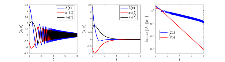
Figure 1: Solution trajectories (the left for 24 and the medium for 25) and their errors (the right) with $p=6$.

3 An Implicit Scheme

From now on, we move to discrete level and consider general nonsmooth $\mu$-convex objective $f$ with $\mu\geqslant 0$. In this setting our primal-dual flow 15a becomes a differential inclusion

$$\gamma x^{\prime}\in-\partial_{x}\mathcal{L}(x,\lambda),$$ (26a)

$$\beta\lambda^{\prime}={}\nabla_{\lambda}\mathcal{L}(x+x^{\prime},\lambda),$$ (26b)

where $\partial_{x}\mathcal{L}(x,\lambda)=\partial f(x)+A^{\top}\lambda$. As discussed in 2.2, well-posedness of the solution to 26b in proper sense is left as a future topic. In what follows, we shall present new primal-dual algorithms based on implicit Euler discretization (this section) and semi-implicit discretization (the next section), respectively. Similar with the continuous level, the tool of Lyapunov function plays important role in convergence rate analysis.

3.1 Implicit discretization

We first consider an implicit Euler scheme for 26a:

$${}v_{k+1}=x_{k+1}+\frac{x_{k+1}-x_{k}}{\alpha_{k}},$$ (27a)

$$\beta_{k}\frac{\lambda_{k+1}-\lambda_{k}}{\alpha_{k}}={}\nabla_{\lambda}\mathcal{L}(v_{k+1},\lambda_{k+1}),$$ (27b)

$$\gamma_{k}\frac{x_{k+1}-x_{k}}{\alpha_{k}}\in-\partial_{x}\mathcal{L}(x_{k+1},\lambda_{k+1}),$$ (27c)

where $\alpha_{k}>0$ denotes the step size and the parameter system 9 is also discretized implicitly

$$\frac{\gamma_{k+1}-\gamma_{k}}{\alpha_{k}}={}\mu-\gamma_{k+1},\quad\frac{\beta_{k+1}-\beta_{k}}{\alpha_{k}}=-\beta_{k+1}.$$ (28)

Let us transform the time discretization 27c to a primal-dual algorithm. From (27c) it follows that

$$\frac{x_{k+1}-x_{k}+\theta_{k}A^{\top}\lambda_{k+1}}{\theta_{k}}\in-\partial f(x_{k+1}),$$ (29)

where $\theta_{k}=\alpha_{k}/\gamma_{k}$. Plugging (27a) into (27b) and using 28, we find

$$\lambda_{k+1}=\lambda_{k}-\frac{1}{\beta_{k}}(Ax_{k}-b)+\frac{1}{\beta_{k+1}}(Ax_{k+1}-b).$$ (30)

Then, combining 29 and 30 gives

$$\frac{x_{k+1}-\widehat{x}_{k}}{\theta_{k}}+\frac{1}{\beta_{k+1}}A^{\top}(Ax_{k+1}-b)+A^{\top}\lambda_{k}\in-\partial f(x_{k+1}),$$

where $\widehat{x}_{k}:=x_{k}+\theta_{k}/\beta_{k}A^{\top}(Ax_{k}-b)$. Consequently, we obtain

$$x_{k+1}={}\mathop{{\mathop{{\rm argmin}}\,}}_{x\in\,{\mathbb{R}}^{n}}\left\{\mathcal{L}(x,\lambda_{k})+\frac{1}{2\beta_{k+1}}\left\lVert{Ax-b}\right\rVert^{2}+\frac{1}{2\theta_{k}}\left\lVert{x-\widehat{x}_{k}}\right\rVert^{2}\right\},$$ (31a)

$$v_{k+1}={}x_{k+1}+(x_{k+1}-x_{k})/\alpha_{k},$$ (31b)

$$\lambda_{k+1}={}\lambda_{k}+\alpha_{k}/\beta_{k}(Av_{k+1}-b).$$ (31c)

Note that in 27c we used only the Lagrangian function $\mathcal{L}(x,\lambda)$ without the augmented term $\left\lVert{Ax-b}\right\rVert^{2}$. But in (31a), the augmented term arises because $\lambda_{k+1}$ and $x_{k+1}$ are coupled with each other in the implicit discretization 27c.

The method 31a is very close the the proximal ALM and the key is to solve the subproblem (31a) with respect to the primal variable $x_{k+1}$. On the other hand, from 29 we observe that $x_{k+1}={\bf prox}_{\theta_{k}f}(x_{k}-\theta_{k}A^{\top}\lambda_{k+1})$. Putting this back to 31c gives a nonlinear equation in terms of the multiplier $\lambda_{k+1}$:

$$\beta_{k+1}\lambda_{k+1}-A{\bf prox}_{\theta_{k}f}\left(x_{k}-\theta_{k}A^{\top}\lambda_{k+1}\right)-z_{k}=0,$$ (32)

where $z_{k}=\beta_{k+1}\left(\lambda_{k}-\beta_{k}^{-1}(Ax_{k}-b)\right)-b$. As discussed later in Section 4.1, instead of computing $x_{k+1}$ from (31a), we apply the semi-smooth Newton method [32] to 32 to obtain $\lambda_{k+1}$ and then update $x_{k+1}$.

Remark 3.1.

For a better understanding of 31a and 32 , we give an operator perspective. Notice that 27a is a nonlinear saddle-point type equation with respect to $x_{k+1}$ and $\lambda_{k+1}$:

$$\mathcal{A}\begin{pmatrix}x_{k+1}\\ \lambda_{k+1}\end{pmatrix}=r_{k}\quad\text{where}\quad\mathcal{A}=\begin{pmatrix}\,{\rm Id}+\theta_{k}\partial f&A^{\top}\\ -A&\beta_{k+1}\,{\rm Id}\end{pmatrix}.$$ (33)

Formally, we have the following factorizations:

$$\mathcal{A}={} \begin{pmatrix}\,{\rm Id}&A^{\top}/\beta_{k+1}\\ O&\,{\rm Id}\end{pmatrix}\begin{pmatrix}\mathcal{P}&O\\ O&\beta_{k+1}\,{\rm Id}\end{pmatrix}\begin{pmatrix}\,{\rm Id}&O\\ -A/\beta_{k+1}&\,{\rm Id}\end{pmatrix},$$

$$\mathcal{A}={} \begin{pmatrix}\,{\rm Id}&O\\ (\,{\rm Id}+\theta_{k}\partial f)^{-1}(-A)&\,{\rm Id}\end{pmatrix}\begin{pmatrix}\,{\rm Id}+\theta_{k}\partial f&O\\ O&\mathcal{S}\end{pmatrix}\begin{pmatrix}\,{\rm Id}&(\,{\rm Id}+\theta_{k}\partial f)^{-1}(-A^{\top})\\ O&\,{\rm Id}\end{pmatrix},$$

where $\mathcal{P}=\,{\rm Id}+\theta_{k}\partial f+A^{\top}A/\beta_{k+1}$ and

$$\mathcal{S}=\beta_{k+1}\,{\rm Id}-A(\,{\rm Id}+\theta_{k}\partial f)^{-1}(-A^{\top})=\beta_{k+1}\,{\rm Id}-A{\bf prox}_{\theta_{k}f}(-A^{\top})$$

is nothing but the Schur complement. Hence, to solve 33, we can compute

$$\mathcal{P}^{-1}=\left(\,{\rm Id}+\theta_{k}\partial f+A^{\top}A/\beta_{k+1}\right)^{-1},$$

which corresponds to the augmented Lagrangian method 31a. On the other hand, one can calculate

$$\mathcal{S}^{-1}=\left(\beta_{k+1}\,{\rm Id}-A{\bf prox}_{\theta_{k}f}(-A^{\top})\right)^{-1},$$

which is equivalent to solve the nonlinear equation 32. ∎

Below the implicit scheme 27c (i.e., the method 31a) has been rewritten as an algorithm framework, which is called the implicit primal-dual (Im-PD) method. According to Lemma 3.1 below, we have global linear rate $(1+\widehat{\alpha})^{-k}$ as long as the step size is bounded below $\alpha_{k}\geqslant\widehat{\alpha}>0$, and superlinear convergence follows if $\alpha_{k}\to\infty$. Note that this holds even for convex case $\mu=0$. In fact, the fully implicit scheme 27b inherits the exponential decay 16 from the continuous level, and thus we have the contraction 35 which has no restriction on the step size $\alpha_{k}$. Besides, the strong convexity constant $\mu$ of the objective $f$ is not necessarily needed since one can set $\mu=0$ in 27b and this leaves the final rate in Lemma 3.1 unchanged.

Algorithm 1 Im-PD method for problem 1 with $f$ being $\mu$-convex ($\mu\geqslant 0$)

0:  $\gamma_{0}>0,\,\beta_{0}>0,\,x_{0}\in\,{\mathbb{R}}^{n},\,\lambda_{0}\in\,{\mathbb{R}}^{m}$.

1:  for $k=0,1,\ldots$ do

2:     Choose the step size $\alpha_{k}>0$.

3:     Update $\displaystyle\beta_{k+1}=\beta_{k}/(1+\alpha_{k})$ and $\displaystyle\gamma_{k+1}=(\mu\alpha_{k}+\gamma_{k})/(1+\alpha_{k})$.

4:     Set $\displaystyle\theta_{k}={}\alpha_{k}/\gamma_{k}$ and $\displaystyle z_{k}={}\beta_{k+1}\left(\lambda_{k}-\beta_{k}^{-1}(Ax_{k}-b)\right)-b$.

5:     Solve $\lambda_{k+1}$ from 32 via the SsN iteration (55) with the line search procedure (56).

6:     Update $x_{k+1}={\bf prox}_{\theta_{k}f}\left(x_{k}-\theta_{k}A^{\top}\lambda_{k+1}\right)$.

7:  end for

3.2 Convergence rate

We now prove the convergence rate of the implicit scheme 27b (i.e. Algorithm 1) via a discrete analogue to 11:

$$\mathcal{E}_{k}:=\mathcal{L}(x_{k},\lambda^{*})-\mathcal{L}(x^{*},\lambda_{k})+\frac{\beta_{k}}{2}\left\lVert{\lambda_{k}-\lambda^{*}}\right\rVert^{2}+\frac{\gamma_{k}}{2}\left\lVert{x_{k}-x^{*}}\right\rVert^{2},$$ (34)

where $(x^{*},\lambda^{*})\in\Omega^{*}$ and $\{(x_{k},\lambda_{k},\gamma_{k},\beta_{k})\}\in\bm{V}$.

Lemma 3.1.

Assume $f$ is $\mu$-convex with $\mu\geqslant 0$. Let $\{(x_{k},\lambda_{k},\gamma_{k},\beta_{k})\}$ be generated by Algorithm 1 with arbitrary step size $\alpha_{k}>0$, then we have the contraction

$$\mathcal{E}_{k+1}-\mathcal{E}_{k}\leqslant-\alpha_{k}\mathcal{E}_{k+1},\quad\text{for all }\,k\in\mathbb{N}.$$ (35)

Moreover, there holds that

$${}\left\lVert{Ax_{k}-b}\right\rVert\leqslant\mathcal{R}_{0}\times\prod_{i=0}^{k-1}\frac{1}{1+\alpha_{i}},$$ (36)

$$0\leqslant\mathcal{L}(x_{k},\lambda^{*})-\mathcal{L}(x^{*},\lambda_{k})\leqslant\mathcal{E}_{0}\times\prod_{i=0}^{k-1}\frac{1}{1+\alpha_{i}},$$ (37)

$${}\left\lvert{f(x_{k})-f(x^{*})}\right\rvert\leqslant\left(\mathcal{E}_{0}+\mathcal{R}_{0}\left\lVert{\lambda^{*}}\right\rVert\right)\times\prod_{i=0}^{k-1}\frac{1}{1+\alpha_{i}},$$ (38)

where $\mathcal{R}_{0}:=\sqrt{2\beta_{0}\mathcal{E}_{0}}+\beta_{0}\left\lVert{\lambda_{0}-\lambda^{*}}\right\rVert+\left\lVert{Ax_{0}-b}\right\rVert$.

Proof.

To prove 35, we mimic the continuous level (cf. Section 2) but replace the derivative with the difference $\mathcal{E}_{k+1}-\mathcal{E}_{k}=I_{1}+I_{2}+I_{3}$, where

$$\left\{\begin{split}I_{1}:={}&\mathcal{L}(x_{k+1},\lambda^{*})-\mathcal{L}(x_{k},\lambda^{*}),\\ I_{2}:={}&\frac{\beta_{k+1}}{2}\left\lVert{\lambda_{k+1}-\lambda^{*}}\right\rVert^{2}-\frac{\beta_{k}}{2}\left\lVert{\lambda_{k}-\lambda^{*}}\right\rVert^{2},\\ I_{3}:={}&\frac{\gamma_{k+1}}{2}\left\lVert{x_{k+1}-x^{*}}\right\rVert^{2}-\frac{\gamma_{k}}{2}\left\lVert{x_{k}-x^{*}}\right\rVert^{2}.\end{split}\right.$$ (39)

Let $p_{k+1}=(x_{k+1}-(x_{k}-\theta_{k}A^{\top}\lambda_{k+1}))/\theta_{k}$, then by 29, we have $A^{\top}\lambda^{*}-p_{k+1}\in\partial\mathcal{L}(x_{k+1},\lambda^{*})$. Since $\mathcal{L}(\cdot,\lambda^{*})$ is $\mu$-convex, by 5 we have

$$I_{1}\leqslant{}\left\langle{A^{\top}\lambda^{*}-p_{k+1},x_{k+1}-x_{k}}\right\rangle-\frac{\mu}{2}\left\lVert{x_{k+1}-x_{k}}\right\rVert^{2}.$$

Shift $\lambda^{*}$ to $\lambda_{k+1}$ and use the relation

$$p_{k+1}-A^{\top}\lambda_{k+1}=x_{k+1}-x_{k}$$ (40)

to lighten the previous estimate as follows

$$I_{1}\leqslant-\left\langle{Ax_{k+1}-Ax_{k},\lambda_{k+1}-\lambda^{*}}\right\rangle,$$ (41)

where we dropped the surplus negative term $-\left\lVert{x_{k+1}-x_{k}}\right\rVert^{2}$.

Then we focus on $I_{2}$ and $I_{3}$. By 28, a direct computation yields

$$\begin{split}I_{2}={}&-\frac{\alpha_{k}\beta_{k+1}}{2}\left\lVert{\lambda_{k+1}-\lambda^{*}}\right\rVert^{2}+\frac{\beta_{k}}{2}\left(\left\lVert{\lambda_{k+1}-\lambda^{*}}\right\rVert^{2}-\left\lVert{\lambda_{k}-\lambda^{*}}\right\rVert^{2}\right)\\ ={}&-\frac{\alpha_{k}\beta_{k+1}}{2}\left\lVert{\lambda_{k+1}-\lambda^{*}}\right\rVert^{2}+\beta_{k}\left\langle{\lambda_{k+1}-\lambda_{k},\lambda_{k+1}-\lambda^{*}}\right\rangle-\frac{\beta_{k}}{2}\left\lVert{\lambda_{k+1}-\lambda_{k}}\right\rVert^{2}.\end{split}$$

Plugging (27b) into the second term and dropping the last negative term lead to

$$I_{2}\leqslant-\frac{\alpha_{k}\beta_{k+1}}{2}\left\lVert{\lambda_{k+1}-\lambda^{*}}\right\rVert^{2}+\alpha_{k}\left\langle{Ax_{k+1}-b,\lambda_{k+1}-\lambda^{*}}\right\rangle+\left\langle{Ax_{k+1}-Ax_{k},\lambda_{k+1}-\lambda^{*}}\right\rangle.$$ (42)

Similarly, we have

$$\begin{split}I_{3}={}&\frac{\gamma_{k+1}-\gamma_{k}}{2}\left\lVert{x_{k+1}-x^{*}}\right\rVert^{2}+\frac{\gamma_{k}}{2}\left(\left\lVert{x_{k+1}-x^{*}}\right\rVert^{2}-\left\lVert{x_{k}-x^{*}}\right\rVert^{2}\right)\\ ={}&\frac{\alpha_{k}}{2}(\mu-\gamma_{k+1})\left\lVert{x_{k+1}-x^{*}}\right\rVert^{2}+\gamma_{k}\left\langle{x_{k+1}-x_{k},(x_{k+1}+x_{k})/2-x^{*}}\right\rangle.\end{split}$$ (43)

By 40, we divide the last term by that

$$\gamma_{k}\left\langle{x_{k+1}-x_{k},(x_{k+1}+x_{k})/2-x^{*}}\right\rangle={} \gamma_{k}\left\langle{x_{k+1}-x_{k},x_{k+1}-x^{*}}\right\rangle-\frac{\gamma_{k}}{2}\left\lVert{x_{k+1}-x_{k}}\right\rVert^{2}$$

$$= -\alpha_{k}\left\langle{A^{\top}\lambda_{k+1}-p_{k+1},x_{k+1}-x^{*}}\right\rangle-\frac{\gamma_{k}}{2}\left\lVert{x_{k+1}-x_{k}}\right\rVert^{2}.$$

Since 29 implies $A^{\top}\lambda_{k+1}-p_{k+1}\in\partial\mathcal{L}(x_{k+1},\lambda_{k+1})$, we obtain

$$\begin{split}&-\alpha_{k}\left\langle{A^{\top}\lambda_{k+1}-p_{k+1},x_{k+1}-x^{*}}\right\rangle\\ \leqslant{}&\alpha_{k}(\mathcal{L}(x^{*},\lambda_{k+1})-\mathcal{L}(x_{k+1},\lambda_{k+1}))-\frac{\mu\alpha_{k}}{2}\left\lVert{x_{k+1}-x^{*}}\right\rVert^{2}\\ ={}&\alpha_{k}(\mathcal{L}(x^{*},\lambda_{k+1})-\mathcal{L}(x_{k+1},\lambda^{*}))-\frac{\mu\alpha_{k}}{2}\left\lVert{x_{k+1}-x^{*}}\right\rVert^{2}-\alpha_{k}\left\langle{Ax_{k+1}-b,\lambda_{k+1}-\lambda^{*}}\right\rangle,\end{split}$$

which promises the following bound

$$\begin{split}I_{3}\leqslant{}&\alpha_{k}(\mathcal{L}(x^{*},\lambda_{k+1})-\mathcal{L}(x_{k+1},\lambda^{*}))-\frac{\alpha_{k}\gamma_{k+1}}{2}\left\lVert{x_{k+1}-x^{*}}\right\rVert^{2}\\ {}&\quad-\alpha_{k}\left\langle{Ax_{k+1}-b,\lambda_{k+1}-\lambda^{*}}\right\rangle-\frac{\gamma_{k}}{2}\left\lVert{x_{k+1}-x_{k}}\right\rVert^{2}.\end{split}$$ (44)

Consequently, combining 41, 42 and 44 proves 35.

From 35 we conclude that $\mathcal{E}_{k}\leqslant\mathcal{E}_{0}\times\prod_{i=0}^{k-1}\frac{1}{1+\alpha_{i}}$, which together with 34 implies (37) and that $\beta_{0}\left\lVert{\lambda_{k}-\lambda^{*}}\right\rVert^{2}\leqslant 2\mathcal{E}_{0}$. Hence it is sufficient to prove (36) and (38). From 30 follows that

$$\lambda_{k}-\frac{1}{\beta_{k}}(Ax_{k}-b)=\lambda_{0}-\frac{1}{\beta_{0}}(Ax_{0}-b)\quad\text{for all }k\in\mathbb{N}.$$ (45)

Then the estimate (36) is derived as below

$$\begin{split}\left\lVert{Ax_{k}-b}\right\rVert={}&\beta_{k}\left\lVert{\lambda_{k}-\lambda_{0}+\beta_{0}^{-1}(Ax_{0}-b)}\right\rVert\leqslant{}\beta_{k}\left\lVert{\lambda_{k}-\lambda_{0}}\right\rVert+\frac{\beta_{k}}{\beta_{0}}\left\lVert{Ax_{0}-b}\right\rVert\\ \leqslant{}&\beta_{k}\left\lVert{\lambda_{k}-\lambda^{*}}\right\rVert+\beta_{k}\left\lVert{\lambda_{0}-\lambda^{*}}\right\rVert+\frac{\beta_{k}}{\beta_{0}}\left\lVert{Ax_{0}-b}\right\rVert\leqslant\frac{\beta_{k}}{\beta_{0}}\mathcal{R}_{0}.\end{split}$$

In addition, it is clear that

$$0\leqslant\mathcal{L}(x_{k},\lambda^{*})-\mathcal{L}(x^{*},\lambda_{k})=f(x_{k})-f(x^{*})+\left\langle{\lambda^{*},Ax_{k}-b}\right\rangle\leqslant\mathcal{L}(x_{k},\lambda^{*})-\mathcal{L}(x^{*},\lambda_{k}),$$

and thus

$$\left\lvert{f(x_{k})-f(x^{*})}\right\rvert\leqslant\left\lVert{\lambda^{*}}\right\rVert\left\lVert{Ax_{k}-b}\right\rVert+\mathcal{L}(x_{k},\lambda^{*})-\mathcal{L}(x^{*},\lambda_{k})\leqslant\frac{\beta_{k}}{\beta_{0}}\left(\mathcal{E}_{0}+\left\lVert{\lambda^{*}}\right\rVert\mathcal{R}_{0}\right).$$

This establishes (38) and completes the proof of this theorem. ∎

4 Composite Optimization

In this section, we move to the composite case

$$\mathop{\min}_{x\in\,{\mathbb{R}}^{n}}f(x)=h(x)+g(x)\quad{\rm s.t.~{}}Ax=b,$$ (46)

where $h$ is $L$-smooth and $\mu$-convex with $\mu\geqslant 0$ and $g$ is properly closed convex (possibly nonsmooth). Instead of the fully implicit scheme 27b, to utilize the composite structure of $f=g+h$, we adopt a semi-implicit discretization that corresponds to the operator splitting (also known as the forward-backward technique). Note also that if $h$ is only convex but the nonsmooth part $g$ is $\mu$-convex, then we can always consider $f=\widehat{h}+\widehat{g}$ with $\widehat{h}(x)=h(x)+\mu/2\left\lVert{x}\right\rVert^{2}$ and $\widehat{g}(x)=g(x)-\mu/2\left\lVert{x}\right\rVert^{2}$, which agrees with the current assumption for 46 and ${\bf prox}_{\widehat{g}}$ can be computed by ${\bf prox}_{g}$ (cf. [63, Section 2.2]).

4.1 A semi-implicit primal-dual proximal gradient method

Based on 27b, we replace $\partial_{x}\mathcal{L}(x_{k+1},\lambda_{k+1})$ with $\nabla h(x_{k})+\partial g(x_{k+1})+A^{\top}\lambda_{k+1}$ to obtain

$${}v_{k+1}=x_{k}+\frac{x_{k+1}-x_{k}}{\alpha_{k}},$$ (47a)

$$\beta_{k+1}\frac{\lambda_{k+1}-\lambda_{k}}{\alpha_{k}}={}\nabla_{\lambda}\mathcal{L}(v_{k+1},\lambda_{k+1}),$$ (47b)

$$\gamma_{k+1}\frac{x_{k+1}-x_{k}}{\alpha_{k}}\in-\nabla h(x_{k})-\partial g(x_{k+1})-A^{\top}\lambda_{k+1},$$ (47c)

where the parameter system 9 is discretized explicitly by

$$\frac{\gamma_{k+1}-\gamma_{k}}{\alpha_{k}}={}\mu-\gamma_{k},\quad\frac{\beta_{k+1}-\beta_{k}}{\alpha_{k}}=-\beta_{k}.$$ (48)

Similar as before, we can rewrite 47b as a primal-dual formulation:

$$x_{k+1}={}\mathop{{\mathop{{\rm argmin}}\,}}_{x\in\,{\mathbb{R}}^{n}}\left\{f(x)+\left\langle{\nabla h(x_{k})+A^{\top}\lambda_{k},x}\right\rangle+\frac{1}{2\beta_{k+1}}\left\lVert{Ax-b}\right\rVert^{2}+\frac{1}{2\eta_{k}}\left\lVert{x-\widehat{x}_{k}}\right\rVert^{2}\right\},$$ (49a)

$$v_{k+1}={}x_{k}+(x_{k+1}-x_{k})/\alpha_{k},$$ (49b)

$$\lambda_{k+1}={}\lambda_{k}+\alpha_{k}/\beta_{k+1}(Av_{k+1}-b),$$ (49c)

where $\eta_{k}=\alpha_{k}/\gamma_{k+1}$ and $\widehat{x}_{k}=x_{k}+\eta_{k}/\beta_{k}A^{\top}(Ax_{k}-b)$. In (49a), the smooth part $h$ has been linearized while the nonsmooth part $g$ uses implicit discretization. This is similar with the proximal gradient method [7, 63], and we have to impose proper restriction on the step size $\alpha_{k}$ (see Algorithm 2).

Notice also that the subproblem (49a) with respect to the primal variable $x_{k+1}$ is not easy to solve. From (47c) we have $x_{k+1}={\bf prox}_{\eta_{k}g}\left(x_{k}-\eta_{k}\nabla h(x_{k})-\eta_{k}A^{\top}\lambda_{k+1}\right)$, and putting this into (49c) gives

$$\beta_{k+1}\lambda_{k+1}-A{\bf prox}_{\eta_{k}g}\left(y_{k}-\eta_{k}A^{\top}\lambda_{k+1}\right)=z_{k},$$ (50)

where $y_{k}={}x_{k}-\eta_{k}\nabla h(x_{k})$ and $z_{k}={}\beta_{k+1}\left(\lambda_{k}-\beta_{k}^{-1}(Ax_{k}-b)\right)-b$. Below, we present a semi-smooth Newton method to solve the nonlinear equation 50 in terms of the multiplier $\lambda_{k+1}$. This can be very efficient for some practical cases that (i) the multiplier has lower dimension than the primal variable; (ii) the problem 50 itself possesses some nice properties such as semi-smoothness and simple closed proximal formulation of $g$; (iii) efficient iterative methods for updating the Newton direction can be considered if there has sparsity.

4.1.1 A semi-smooth Newton method for the subproblem 50

Define a mapping $F_{k}:\,{\mathbb{R}}^{m}\to\,{\mathbb{R}}^{m}$ by that

$$F_{k}(\lambda):=\beta_{k+1}\lambda-A{\bf prox}_{\eta_{k}g}\left(y_{k}-\eta_{k}A^{\top}\lambda\right)-z_{k}\quad\forall\,\lambda\in\,{\mathbb{R}}^{m}.$$ (51)

Then (50) is equivalent to $F_{k}(\lambda_{k+1})=0$. By Moreau’s identity (cf. [5, Theorem 6.45])

$${\bf prox}_{\eta g}(x)+\eta{\bf prox}_{g^{*}/\eta}(x/\eta)=x,$$ (52)

where $g^{*}$ denotes the conjugate function of $g$, we find that $F_{k}(\lambda)=\nabla\mathcal{F}_{k}(\lambda)$, where

$$\small\begin{split}\mathcal{F}_{k}(\lambda):={}&\frac{\beta_{k+1}}{2}\left\lVert{\lambda}\right\rVert^{2}-\left\langle{z_{k},\lambda}\right\rangle+g^{*}\left({\bf prox}_{g^{*}/\eta_{k}}(y_{k}/\eta_{k}-A^{\top}\lambda)\right)+\frac{1}{2\eta_{k}}\left\lVert{{\bf prox}_{\eta_{k}g}(y_{k}-\eta_{k}A^{\top}\lambda)}\right\rVert^{2}.\end{split}$$ (53)

Let $\partial{\bf prox}_{\eta_{k}g}(\lambda)$ be the generalized Clarke subdifferential [24] of ${\bf prox}_{\eta_{k}g}(\lambda)$. If $P_{k}(\lambda)\in\partial{\bf prox}_{\eta_{k}g}\left(y_{k}-\eta_{k}A^{\top}\lambda\right)$ is symmetric (this is indeed true when $g$ is either the indicator function or the support function for some nonempty convex polyhedral [38]), then for any $\lambda\in\,{\mathbb{R}}^{m}$ we can define an SPD matrix

$$JF_{k}(\lambda):=\beta_{k+1}I+\eta_{k}AP_{k}(\lambda)A^{\top}\in\,{\mathbb{R}}^{m\times m}.$$ (54)

The semi-smooth Newton (SsN) method for solving (50) reads as follows: given an initial guess $\lambda^{0}\in\,{\mathbb{R}}^{m}$, do the iteration

$$\lambda^{j+1}=\lambda^{j}-\left[JF_{k}(\lambda^{j})\right]^{-1}F_{k}(\lambda^{j}),\quad j\geq 0.$$ (55)

Theoretically, it possesses local superlinear convergence provided that $F_{k}$ is semismooth [66, 67]. Practically, it can be terminated under some suitable criterion and for global convergence, a line search procedure [27] shall be supplemented: given a Newton direction $d^{j}=-\left[JF_{k}(\lambda^{j})\right]^{-1}F_{k}(\lambda^{j})$ at step $j$, find the smallest nonnegative integer $r\in\mathbb{N}$ such that

$$\mathcal{F}_{k}(\lambda^{j}+\delta^{r}d^{j})\leqslant\mathcal{F}_{k}(\lambda^{j})+\nu\delta^{r}\left\langle{F_{k}(\lambda^{j}),d^{j}}\right\rangle,$$ (56)

where $\nu\in(0,1/2),\,\delta\in(0,1]$ and $\mathcal{F}_{k}$ has been defined in 53. Generally the inverse operation $\left[JF_{k}(\lambda^{j})\right]^{-1}$ in 55 shall be approximated by some iterative process such as the (preconditioned) conjugate gradient method [69]. For more discussions about the linear solver for $d^{j}$, we refer to Section 5.1.2.

Below we summarize the semi-implicit scheme 47c as an algorithm framework, which is called the semi-implicit primal-dual proximal gradient (Semi-PDPG) method. As suggested later by Theorem 4.1, the step size $\alpha_{k}$ is determined simply by $\alpha_{k}(L+\gamma_{k+1})=\gamma_{k+1}$, which promises the convergence rate $\mathcal{O}(\min\{L/k,(1+\mu/L)^{-k}\})$ (cf. 61).

Algorithm 2 Semi-PDPG method for 46 with $h$ being $L$-smooth and $\mu$-convex $(\mu\geqslant 0)$

0:  $\gamma_{0}>0,\,\beta_{0}>0,\,x_{0}\in\,{\mathbb{R}}^{n},\,\lambda_{0}\in\,{\mathbb{R}}^{m}$.

1:  for $k=0,1,\ldots$ do

2:     Set $\sigma_{k}=L+2\gamma_{k}-\mu$ and $\Delta_{k}=\sigma_{k}+\sqrt{\sigma_{k}^{2}+4\gamma_{k}(\mu-\gamma_{k})}$.

3:     Compute the step size $\alpha_{k}=2\gamma_{k}/\Delta_{k}\in(0,1)$.

4:     Update $\displaystyle\beta_{k+1}=\beta_{k}(1-\alpha_{k})$ and $\displaystyle\gamma_{k+1}=\mu\alpha_{k}+(1-\alpha_{k})\gamma_{k}$.

5:     Set $\displaystyle\eta_{k}={}\alpha_{k}/\gamma_{k+1}$ and $y_{k}=x_{k}-\eta_{k}\nabla h(x_{k})$.

6:     Set $\displaystyle z_{k}={}\beta_{k+1}\left(\lambda_{k}-\beta_{k}^{-1}(Ax_{k}-b)\right)-b$.

7:     Solve $\lambda_{k+1}$ from (50) via the SsN iteration (55) with the line search procedure (56).

8:     Update $x_{k+1}={\bf prox}_{\eta_{k}g}\left(y_{k}-\eta_{k}A^{\top}\lambda_{k+1}\right)$.

9:  end for

4.2 Proof of the convergence rate

To move on, the following two lemmas are needed.

Lemma 4.1.

Assume $h$ is $L$-smooth and $\mu$-convex with $\mu\geqslant 0$ and $g$ is properly closed convex. Let $\{(x_{k},\lambda_{k},\gamma_{k},\beta_{k})\}$ be generated by 47b and 48, then for all $y\in\,{\mathbb{R}}^{n}$,

$$\begin{split}{}&\mathcal{L}(x_{k+1},\lambda_{k+1})-\mathcal{L}(y,\lambda_{k+1})+\frac{\gamma_{k+1}}{\alpha_{k}}\left\langle{x_{k+1}-x_{k},x_{k}-y}\right\rangle\\ \leqslant{}&-\frac{\mu}{2}\left\lVert{y-x_{k}}\right\rVert^{2}+\frac{L\alpha_{k}-2\gamma_{k+1}}{2\alpha_{k}}\left\lVert{x_{k+1}-x_{k}}\right\rVert^{2}.\end{split}$$ (57)

Proof.

Define $\phi(x):=h(x)+\left\langle{\lambda_{k+1},Ax-b}\right\rangle$ for all $x\in\,{\mathbb{R}}^{n}$. As $h$ is $L$-smooth and $\mu$-convex, there holds that

$$\begin{split}\phi(x_{k})-\phi(y)+\left\langle{\nabla\phi(x_{k}),y-x_{k}}\right\rangle\leqslant&-\frac{\mu}{2}\left\lVert{y-x_{k}}\right\rVert^{2},\\ \phi(x_{k+1})-\phi(x_{k})-\left\langle{\nabla\phi(x_{k}),x_{k+1}-x_{k}}\right\rangle\leqslant{}&\frac{L}{2}\left\lVert{x_{k+1}-x_{k}}\right\rVert^{2}.\end{split}$$

In addition, by (47c), we have

$$\gamma_{k+1}\frac{x_{k}-x_{k+1}}{\alpha_{k}}-\nabla\phi(x_{k})\in\partial g(x_{k+1}),$$

and it follows that

$$\begin{split}{}&g(x_{k+1})-g(y)\leqslant\left\langle{\gamma_{k+1}\frac{x_{k}-x_{k+1}}{\alpha_{k}}-\nabla\phi(x_{k}),x_{k+1}-y}\right\rangle\\ ={}&\frac{\gamma_{k+1}}{\alpha_{k}}\left\langle{x_{k}-x_{k+1},x_{k}-y}\right\rangle-\left\langle{\nabla\phi(x_{k}),x_{k+1}-y}\right\rangle-\frac{\gamma_{k+1}}{\alpha_{k}}\left\lVert{x_{k+1}-x_{k}}\right\rVert^{2}.\end{split}$$

Collecting the above estimates and using the fact $\mathcal{L}(\cdot,\lambda)=\phi(\cdot)+g(\cdot)$, we obtain 57 and conclude the proof. ∎

Recall $\gamma_{\min}$ defined in 18 and for later use we set $\gamma_{\max}:=\max\{\gamma_{0},\mu\}$.

Lemma 4.2.

Let $\{(\gamma_{k},\beta_{k})\}$ be defined by 48 with $\alpha_{k}(L+\gamma_{k+1})\leqslant 2\gamma_{k+1}$, then $\alpha_{k}\in(0,1]$ for all $k\in\mathbb{N}$. Moreover, if $\alpha_{k}(L+\gamma_{k+1})=\gamma_{k+1}$ then

$$\prod_{i=0}^{k-1}(1-\alpha_{i})\leqslant\min\left\{\frac{L+\gamma_{\max}}{\gamma_{0}k+L+\gamma_{\max}},\,\left(\frac{L}{L+\gamma_{\min}}\right)^{k}\right\}.$$ (58)

Proof.

Let us first verify the existence of the sequence $\{\alpha_{k}\}\subset(0,1]$. As $\alpha_{k}(L+\gamma_{k+1})\leqslant 2\gamma_{k+1}$ and $\gamma_{k+1}=\gamma_{k}+\alpha_{k}(\mu-\gamma_{k})$ (cf. 48), we obtain $\psi_{k}(\alpha_{k}):=(\mu-\gamma_{k})\alpha_{k}^{2}+(L+3\gamma_{k}-2\mu)\alpha_{k}-2\gamma_{k}\leqslant 0$. As $\gamma_{0}>0$, we have $\psi_{0}(0)=-2\gamma_{0}<0$ and $\psi_{0}(1)=L-\mu\geqslant 0$. Hence, there must be at least one (actually unique) root $\alpha^{*}\in(0,1]$ of $\psi_{0}(\alpha)=0$. Hence, any $\alpha_{0}\in(0,\alpha^{*}]$ satisfies $\alpha_{0}(L+\gamma_{1})\leqslant 2\gamma_{1}$. Repeating this process for $\psi_{k}(\alpha)$ and noticing that $\gamma_{k}>0$ yield the existence of $\alpha_{k}\in(0,1]$ for all $k\geqslant 1$.

From 48 we have $\beta_{k}=\beta_{0}\prod_{i=0}^{k-1}(1-\alpha_{i})$. It remains to investigate the asymptotic decay behavior of $\beta_{k}$ with $\alpha_{k}(L+\gamma_{k+1})=\gamma_{k+1}$. Let us start from the identity

$$\frac{1}{\beta_{k+1}}-\frac{1}{\beta_{k}}=\frac{\beta_{k}-\beta_{k+1}}{\beta_{k}\beta_{k+1}}=\frac{\alpha_{k}}{\beta_{k+1}}.$$

Besides, we have

$$\frac{\gamma_{k+1}}{\gamma_{k}}\geqslant 1-\alpha_{k}=\frac{\beta_{k+1}}{\beta_{k}}\quad\Longrightarrow\quad\gamma_{k}\geqslant\frac{\gamma_{0}}{\beta_{0}}\beta_{k}.$$

It follows from this and the relation $\alpha_{k}(L+\gamma_{k+1})=\gamma_{k+1}$ that

$$\frac{1}{\beta_{k+1}}-\frac{1}{\beta_{k}}\geqslant\frac{\gamma_{0}\alpha_{k}}{\beta_{0}\gamma_{k+1}}=\frac{\gamma_{0}}{\beta_{0}(L+\gamma_{k+1})}\geqslant\frac{\gamma_{0}}{\beta_{0}(L+\gamma_{\max})}.$$

Hence, we get

$$\frac{\beta_{k}}{\beta_{0}}\leqslant\frac{L+\gamma_{\max}}{\gamma_{0}k+L+\gamma_{\max}}.$$ (59)

On the other hand, since $\gamma_{k+1}\geqslant\gamma_{\min}$, we have $\alpha_{k}=\gamma_{k+1}/(L+\gamma_{k+1})\geqslant\gamma_{\min}/(L+\gamma_{\min})$. Therefore, another bound follows

$$\frac{\beta_{k}}{\beta_{0}}=\prod_{i=0}^{k-1}(1-\alpha_{i})\leqslant\left(\frac{L}{L+\gamma_{\min}}\right)^{k}.$$

Combining this with 59 establishes 58 and completes the proof of this lemma. ∎

We now prove the convergence rate of Algorithm 2 by using the Lyapunov function (34).

Theorem 4.1.

Assume $h$ is $L$-smooth and $\mu$-convex with $\mu\geqslant 0$ and $g$ is properly closed convex. Let $\{(x_{k},\lambda_{k},\gamma_{k},\beta_{k})\}$ be generated by 47b and 48 with $\alpha_{k}(L+\gamma_{k+1})\leqslant 2\gamma_{k+1}$, then we have $\{\alpha_{k}\}\subset(0,1]$ and

$$\mathcal{E}_{k+1}-\mathcal{E}_{k}\leqslant-\alpha_{k}\mathcal{E}_{k},\quad\text{for all }\,k\in\mathbb{N}.$$ (60)

Moreover, if $\alpha_{k}(L+\gamma_{k+1})=\gamma_{k+1}$, then it holds that

$$\small{}\mathcal{L}(x_{k},\lambda^{*})-\mathcal{L}(x^{*},\lambda_{k})+\left\lvert{F(x_{k})-F(x^{*})}\right\rvert+\left\lVert{Ax_{k}-b}\right\rVert\leqslant C_{0}\times\min\left\{\frac{L+\gamma_{\max}}{\gamma_{0}k+L+\gamma_{\max}},\,\left(\frac{L}{L+\gamma_{\min}}\right)^{k}\right\},$$ (61)

where $C_{0}:=\mathcal{E}_{0}+\mathcal{R}_{0}(1+\left\lVert{\lambda^{*}}\right\rVert)$ with $\mathcal{R}_{0}:=\sqrt{2\beta_{0}\mathcal{E}_{0}}+\beta_{0}\left\lVert{\lambda_{0}-\lambda^{*}}\right\rVert+\left\lVert{Ax_{0}-b}\right\rVert$.

Proof.

The existence of the step size sequence $\{\alpha_{k}\}\subset(0,1]$ has been proved in Lemma 4.2. Once the contraction (60) is established, we obtain $\mathcal{E}_{k}\leqslant\mathcal{E}_{0}\times\prod_{i=0}^{k-1}(1-\alpha_{i})$, and the estimate 61 can be obtain by using Lemma 4.2 and the same procedure for (36), (37) and (38).

Following the proof of Lemma 3.1, we start from the difference $\mathcal{E}_{k+1}-\mathcal{E}_{k}=I_{1}+I_{2}+I_{3}$, where $I_{1},\,I_{2}$ and $I_{3}$ are defined in 39. By 48, we have

$$\begin{split}I_{2}={}&\frac{\beta_{k+1}-\beta_{k}}{2}\left\lVert{\lambda_{k}-\lambda^{*}}\right\rVert^{2}+\frac{\beta_{k+1}}{2}\left(\left\lVert{\lambda_{k+1}-\lambda^{*}}\right\rVert^{2}-\left\lVert{\lambda_{k}-\lambda^{*}}\right\rVert^{2}\right)\\ ={}&-\frac{\alpha_{k}\beta_{k}}{2}\left\lVert{\lambda_{k}-\lambda^{*}}\right\rVert^{2}+\beta_{k+1}\left\langle{\lambda_{k+1}-\lambda_{k},\lambda_{k+1}-\lambda^{*}}\right\rangle-\frac{\beta_{k+1}}{2}\left\lVert{\lambda_{k+1}-\lambda_{k}}\right\rVert^{2}.\end{split}$$

Plugging (47b) into the second term and dropping the last negative term lead to

$$I_{2}\leqslant-\frac{\alpha_{k}\beta_{k}}{2}\left\lVert{\lambda_{k}-\lambda^{*}}\right\rVert^{2}+\alpha_{k}\left\langle{Av_{k+1}-b,\lambda_{k+1}-\lambda^{*}}\right\rangle.$$ (62)

Similarly, for $I_{3}$, it holds that

$$\begin{split}I_{3}={}&\frac{\gamma_{k+1}-\gamma_{k}}{2}\left\lVert{x_{k}-x^{*}}\right\rVert^{2}+\frac{\gamma_{k+1}}{2}\left(\left\lVert{x_{k+1}-x^{*}}\right\rVert^{2}-\left\lVert{x_{k}-x^{*}}\right\rVert^{2}\right)\\ ={}&\frac{\alpha_{k}(\mu-\gamma_{k})}{2}\left\lVert{x_{k}-x^{*}}\right\rVert^{2}+\gamma_{k+1}\left\langle{x_{k+1}-x_{k},x_{k}-x^{*}}\right\rangle+\frac{\gamma_{k+1}}{2}\left\lVert{x_{k+1}-x_{k}}\right\rVert^{2},\end{split}$$

and invoking Lemma 4.2 gives

$$\begin{split}I_{3}\leqslant{}&\alpha_{k}(\mathcal{L}(x^{*},\lambda_{k+1})-\mathcal{L}(x_{k+1},\lambda_{k+1}))-\frac{\alpha_{k}\gamma_{k}}{2}\left\lVert{x_{k}-x^{*}}\right\rVert^{2}+\frac{L\alpha_{k}-\gamma_{k+1}}{2}\left\lVert{x_{k+1}-x_{k}}\right\rVert^{2}.\end{split}$$

To match the right hand side of (60), we shift $(x_{k+1},\lambda_{k+1})$ to $(x_{k},\lambda_{k+1})$ and then to $(x_{k},\lambda^{*})$ and obtain that

$$I_{3}\leqslant{} \alpha_{k}(\mathcal{L}(x^{*},\lambda_{k})-\mathcal{L}(x_{k},\lambda^{*}))-\frac{\alpha_{k}\gamma_{k}}{2}\left\lVert{x_{k}-x^{*}}\right\rVert^{2}$$

$$\quad-\alpha_{k}\left\langle{Ax_{k}-b,\lambda_{k+1}-\lambda^{*}}\right\rangle+\frac{L\alpha_{k}-\gamma_{k+1}}{2}\left\lVert{x_{k+1}-x_{k}}\right\rVert^{2}$$

$$\quad\qquad+\alpha_{k}(\mathcal{L}(x_{k},\lambda_{k+1})-\mathcal{L}(x_{k+1},\lambda_{k+1})).$$

To offset the last term in the above estimate, we shall divide $I_{1}$ as follows

$$\begin{split}{}&I_{1}=\mathcal{L}(x_{k+1},\lambda^{*})-\mathcal{L}(x_{k},\lambda^{*})\\ ={}&\alpha_{k}(\mathcal{L}(x_{k+1},\lambda_{k+1})-\mathcal{L}(x_{k},\lambda_{k+1}))-\left\langle{Ax_{k+1}-Ax_{k},\lambda_{k+1}-\lambda^{*}}\right\rangle\\ {}&\quad+(1-\alpha_{k})(\mathcal{L}(x_{k+1},\lambda_{k+1})-\mathcal{L}(x_{k},\lambda_{k+1})).\end{split}$$

Applying Lemma 4.2 again implies

$$\begin{split}I_{1}\leqslant{}&\alpha_{k}(\mathcal{L}(x_{k+1},\lambda_{k+1})-\mathcal{L}(x_{k},\lambda_{k+1}))-\left\langle{Ax_{k+1}-Ax_{k},\lambda_{k+1}-\lambda^{*}}\right\rangle\\ {}&\qquad+\frac{1-\alpha_{k}}{2\alpha_{k}}(L\alpha_{k}-2\gamma_{k+1})\left\lVert{x_{k+1}-x_{k}}\right\rVert^{2},\end{split}$$

which together with the relation $v_{k+1}=x_{k}+(x_{k+1}-x_{k})/\alpha_{k}$ yields that

$$\begin{split}I_{1}+I_{3}\leqslant{}&\alpha_{k}(\mathcal{L}(x^{*},\lambda_{k})-\mathcal{L}(x_{k},\lambda^{*}))-\frac{\alpha_{k}\gamma_{k}}{2}\left\lVert{x_{k}-x^{*}}\right\rVert^{2}-\alpha_{k}\left\langle{Av_{k+1}-b,\lambda_{k+1}-\lambda^{*}}\right\rangle\\ {}&\qquad+\frac{\alpha_{k}(L+\gamma_{k+1})-2\gamma_{k+1}}{2\alpha_{k}}\left\lVert{x_{k+1}-x_{k}}\right\rVert^{2}.\end{split}$$ (63)

Consequently, combining this with the estimate 62 for $I_{2}$ implies

$$\begin{split}\mathcal{E}_{k+1}-\mathcal{E}_{k}\leqslant&-\alpha_{k}\mathcal{E}_{k}+\frac{\alpha_{k}(L+\gamma_{k+1})-2\gamma_{k+1}}{2\alpha_{k}}\left\lVert{x_{k+1}-x_{k}}\right\rVert^{2}.\end{split}$$

As $\alpha_{k}(L+\gamma_{k+1})\leqslant 2\gamma_{k+1}$, this establishes (60) and completes the proof. ∎

5 Numerical Experiments

In this part, we investigate practical performances of Algorithms 1 and 2 for the $l_{1}$-$l_{2}$ minimization 64 and the total-variation based image denoising model 73.

5.1 The $l_{1}$-$l_{2}$ minimization

We first consider the linearly constrained $l_{1}$-$l_{2}$ minimization:

$$\min_{x\in\,{\mathbb{R}}^{n}}~{}\frac{\rho}{2}\left\lVert{x}\right\rVert^{2}+\left\lVert{x}\right\rVert_{1}\quad{\rm s.t.~{}}Ax=b,$$ (64)

where $\rho>0,\,b\in\,{\mathbb{R}}^{m}$ and $A\in\,{\mathbb{R}}^{m\times n}$ with $m\ll n$. This is a regularized model for the so-called basis pursuit [21], which corresponds to the limit case $\rho=0$ and is related to compressed sensing [14].

Let $g(x)=\left\lVert{x}\right\rVert_{1}$, then for any $\eta>0$, the proximal mapping ${\bf prox}_{\eta g}(x)={\rm sgn}(x)\odot\max\{|x|-\eta,0\}$ is well known as the soft thresholding operator, with the $i$-th component of $y={\bf prox}_{\eta g}(x)$ being given by $y_{i}={\rm sgn}(x_{i})\max\{|x_{i}|-\eta,0\}$. Here and in what follows, $\odot$ and $\oslash$ stand respectively for element-wise multiplication and division operations. The conjugate function $g^{*}$ of $g$ is the indicator function of the cube $[-1,1]^{n}$ and thus ${\bf prox}_{\eta g^{*}}(x)=\min\left\{\max\{x,-1\},1\right\}$.

5.1.1 Comparison with ALB

There are some well-known Bregman methods for solving 64; see [86, 45, 48, 12]. Both of the two accelerated variants in [45, 48] possess the nonergodic sublinear rate $\mathcal{O}(1/k^{2})$ for the dual objective but the method in [48] involves a subproblem for the primal variable. In contrast, the accelerated linearized Bregman (ALB) method in [45] linearizes the augmented term and admits closed update formulation in each step. More precisely, it reads as follows: given $\lambda_{0},\,\widetilde{\lambda}_{0}\in\,{\mathbb{R}}^{m}$, do the iteration

$$\left\{\begin{split}x_{k+1}={}&{\bf prox}_{g/\rho}\left(-A^{\top}\widetilde{\lambda}_{k}/\rho\right),\\ \lambda_{k+1}={}&\widetilde{\lambda}_{k}+\tau\left(Ax_{k+1}-b\right),\\ \widetilde{\lambda}_{k+1}={}&t_{k}\lambda_{k+1}+(1-t_{k})\lambda_{k},\end{split}\right.$$ (65)

where $t_{k}=(2k+3)/(k+3)$ and $\tau=\rho/\left\lVert{A}\right\rVert^{2}$.

Table 1: Performances of Inexact Semi-PDPG (i.e.,Algorithm 3) and ALB method 65 for solving (64). Here, “direct" and “PCG" mean that the linear system in step 15 of Algorithm 3 is solved respectively by direct method and PCG.

						Inexact Semi-PDPG(direct)				Inexact Semi-PDPG(PCG)				ALB
		$m$		$n$		its	SsN	time(sec)		its	SsN	time(sec)		its	time(sec)
$\rho=0.5$		5e+02		2e+03		21	42	5.20		21	40	3.59		537	4.20
		8e+02		3e+03		21	46	10.76		21	43	11.40		593	10.86
		1e+03		4e+03		21	39	12.33		21	42	12.37		546	16.15
$\rho=0.1$		2e+02		1e+03		20	34	0.70		20	43	1.08		2330	2.68
		5e+02		3e+03		21	37	3.66		19	51	5.66		1967	23.81
		1e+03		5e+03		20	43	15.61		20	47	14.00		2118	81.83
$\rho=0.01$		5e+02		2e+03		19	56	4.50		18	60	5.92		13174	103.54
		9e+02		4e+03		18	56	12.49		22	87	41.76		12712	379.83
		2e+03		8e+03		17	63	87.29		19	82	246.34		13819	1693.99
$\rho=0.005$		8e+02		3e+03		21	86	23.39		19	75	39.25		19793	375.07
		2e+03		6e+03		20	86	153.48		23	126	579.69		20811	1778.27
		3e+03		9e+03		19	83	509.93		24	139	1933.28		21568	6592.60

We apply Algorithm 2 to the problem 64. In this case, as $g$ is piecewise affine, ${\bf prox}_{\eta g}$ is strongly semismooth [32] and so is the nonlinear mapping $F_{k}(\cdot)$ defined by 51. For $\eta>0$ and $x\in\,{\mathbb{R}}^{n}$, define a diagonal matrix

$$P_{\eta}(x)={\rm diag}(p)\in\,{\mathbb{R}}^{n\times n}\quad\text{with }p_{i}=\left\{\begin{aligned} {}&1&&\text{if }\left\lvert{x_{i}}\right\rvert\geqslant\eta,\\ {}&0&&\text{if }\left\lvert{x_{i}}\right\rvert<\eta.\end{aligned}\right.$$ (66)

Then it is easy to see that $P_{\eta}(x)\in\partial{\bf prox}_{\eta g}(x)$, and we obtain a generalized Clarke subgradient for 50:

$$JF_{k}(\lambda)=\beta_{k+1}I+\eta_{k}AP_{\eta_{k}}[v_{k}(\lambda)]A^{\top}\in\,{\mathbb{R}}^{m\times m},$$ (67)

where $v_{k}(\lambda)=y_{k}-\eta_{k}A^{\top}\lambda$. Note that $P_{\eta_{k}}[v_{k}(\lambda)]={\rm diag}(p)$ where $p$ is defined by 66 with $p_{i}\in\{0,1\}$, and thus $JF_{k}(\lambda)$ is always SPD. Moreover, the function 53 becomes

$$\mathcal{F}_{k}(\lambda)={}\frac{\beta_{k+1}}{2}\left\lVert{\lambda}\right\rVert^{2}-\left\langle{z_{k},\lambda}\right\rangle+\frac{1}{2\eta_{k}}\left\lVert{{\bf prox}_{\eta_{k}g}[v_{k}(\lambda)]}\right\rVert^{2}.$$

Algorithm 3 Inexact Semi-PDPG method for the $l_{1}$-$l_{2}$ minimization problem 64

0:  $\gamma_{0}>0,\,\beta_{0}>0,\,\,x_{0}\in\,{\mathbb{R}}^{n}$ and $\lambda_{0}\in\,{\mathbb{R}}^{m}$.

1:  Problem setting: $\rho>0,\,b\in\,{\mathbb{R}}^{m}$ and $A\in\,{\mathbb{R}}^{m\times n}$.

2:  SsN setting: $\nu=0.2,\,\delta=0.9$ and $j_{\max}=10$.

3:  Tolerances: $\mathtt{KKT\_Tol}=10^{-6}$ and $\mathtt{SsN\_Tol}=10^{-8}$.

4:  for $k=0,1,\ldots$ do

5:     Set $\sigma_{k}=2\gamma_{k}$ and $\Delta_{k}=\sigma_{k}+\sqrt{\sigma_{k}^{2}+4\gamma_{k}(\rho-\gamma_{k})}$.

6:     Compute the step size $\alpha_{k}=2\gamma_{k}/\Delta_{k}\in(0,1)$.

7:     Update $\displaystyle\beta_{k+1}=\beta_{k}(1-\alpha_{k})$ and $\displaystyle\gamma_{k+1}=\rho\alpha_{k}+(1-\alpha_{k})\gamma_{k}$.

8:     Set $\displaystyle\eta_{k}={}\alpha_{k}/\gamma_{k+1}$ and $y_{k}=x_{k}-\eta_{k}\rho x_{k}$.

9:     Set $\displaystyle z_{k}={}\beta_{k+1}\left(\lambda_{k}-\beta_{k}^{-1}(Ax_{k}-b)\right)-b$.

10:     Solve $\lambda_{k+1}$ from the nonlinear equation

$$F_{k}(\lambda):=\beta_{k+1}\lambda-A{\bf prox}_{\eta_{k}g}\left(y_{k}-\eta_{k}A^{\top}\lambda\right)-z_{k}=0$$ (68)

via the following SsN iteration with $\lambda=\lambda_{k}$ and $j=0$:

11:     while $\left\lVert{F_{k}(\lambda)}\right\rVert>\mathtt{SsN\_Tol}$ and $j<j_{\max}$ do {SsN iteration}

12:        Compute $v_{k}=y_{k}-\eta_{k}A^{\top}\lambda$.

13:        Find $P_{\eta_{k}}(v_{k})\in\partial{\bf prox}_{\eta_{k}g}(v_{k})$ via 66.

14:        Compute $JF_{k}(\lambda)=\beta_{k+1}I+\eta_{k}AP_{\eta_{k}}(v_{k})A^{\top}$.

15:        Solve $JF_{k}(\lambda)d=-F_{k}(\lambda)$.

16:        Find the smallest integer $r\in\mathbb{N}_{+}$ such that $\mathcal{F}_{k}(\lambda+\delta^{r}d)\leqslant\mathcal{F}_{k}(\lambda)+\nu\delta^{r}\left\langle{F_{k}(\lambda),d}\right\rangle$.

17:        Update $\lambda=\lambda+\delta^{r}d$ and $j=j+1$.

18:     end while

19:     Update $\lambda_{k+1}=\lambda$ and $x_{k+1}={\bf prox}_{\eta_{k}g}\left(y_{k}-\eta_{k}A^{\top}\lambda_{k+1}\right)$.

20:     if ${\rm Res}(k)\leqslant\mathtt{KKT\_Tol}$ then

21:        break

22:     end if

23:  end for

We rewrite Algorithm 2 in Algorithm 3, where a practical inexact setting is considered. The SsN iteration (see lines 11–18 in Algorithm 3) is stopped either $\left\lVert{F_{k}(\lambda)}\right\rVert\leqslant\mathtt{SsN\_Tol}=10^{-8}$ or $j_{\max}=10$. For the line search procedure, we adopt $\nu=0.2$ and $\delta=0.9$. All initial guesses $\beta_{0},\,x_{0}$ and $\lambda_{0}$ are generated randomly, and we chose $\gamma_{0}=\mu+\sigma$ with $\sigma$ obeying the uniform distribution on $[0,1]$. By Theorem 4.1 we the linear rate $2^{-k}$ (with exact computation).

Recall the optimality condition of problem 64: $Ax^{*}=b$ and $x^{*}={\bf prox}_{g}((1-\rho)x^{*}-A^{\top}\lambda^{*})$. Hence, we consider the stopping criterion:

$${\rm Res}(k):=\max\left\{{\rm Res}(x_{k}),{\rm Res}(\lambda_{k})\right\}\leqslant\mathtt{KKT\_Tol}=10^{-6},$$ (69)

where the relative KKT residuals are defined by

$${\rm Res}(\lambda_{k}):=\frac{\left\lVert{Ax_{k}-b}\right\rVert}{1+\left\lVert{b}\right\rVert}\quad\text{and}\quad{\rm Res}(x_{k}):=\frac{\left\lVert{x_{k}-{\bf prox}_{g}\left((1-\rho)x_{k}-A^{\top}\lambda_{k}\right)}\right\rVert}{1+\left\lVert{x_{k}}\right\rVert}.$$

In step 15 of Algorithm 3, we have to solve a linear system and we consider two ways: one is direct method as $m\ll n$ and the other is preconditioned conjugate gradient (PCG) method (cf.[69, Algorithm 9.1]) with diagonal preconditioner. The PCG iteration is stopped either the relative residual is smaller than $10^{-8}$ or the maximal iteration number $5000$ is attained.

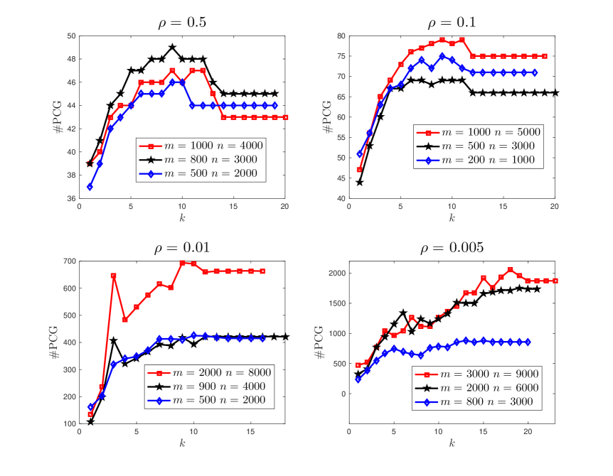
Figure 2: Averaged PCG iterations of Algorithm 3 for solving (64) with different problem size and $\rho$.

Computational results are reported in Table 1, which includes (i) its: the number of total iterations, (ii) SsN: the number of the SsN iterations for the inner problem 68, and (iii) time: the running time (in seconds). To achieve the tolerance 69, the number of iterations of Algorithm 3 is almost $k^{*}=6\ln 10/\ln 2\approx 20$. This can be observed from Table 1. However, as $\rho$ becomes small, the problem 64 itself is more degenerate and the number of iterations of the ALB method grows dramatically.

5.1.2 Performance of the PCG iteration

From Table 1 we see that Algorithm 3 with PCG solver is slightly inferior than that with direct solver, both for total iteration number and running time. We now investigate the performance of the PCG iteration.

The linear system arising from step 15 of Algorithm 3 is $JF_{k}(\lambda)d=-F_{k}(\lambda)$, where $JF_{k}(\cdot)=\beta_{k+1}I+\eta_{k}\mathcal{A}_{0}(\cdot)$ is defined by 67 and $\mathcal{A}_{0}(\cdot)$ is symmetric semi-positive definite. Note that $JF_{k}(\cdot)$ is always SPD but also nearly singular as $\beta_{k+1}\to 0$. Hence, the iteration number will increase as $k$ does. Fortunately, for large $k$, we may expect that $F_{k}(\cdot)$ is close to zero (as the algorithm converges) and the nearly singular property is not a serious problem.

Recall that we used the diagonal preconditioner, i.e., Jacobi iteration, and the terminal criterion is relative residual $\leqslant 10^{-8}$, with the maximal iteration number $5000$. In every $k$-th step of Algorithm 3, we record the PCG iteration $\#_{k,j}$ of the $j$-th SsN iteration and obtain an averaged number $\#_{k}=\frac{1}{s_{k}}\sum_{j=1}^{s_{k}}\#_{k,j}$, where $s_{k}$ denotes the number of SsN iterations for solving the subproblem 68.

In Figure 2, we plot the averaged PCG iterations of Algorithm 3 with the same problem size and $\rho$ used in Table 1. As predicted above, due to the nearly singular property, the PCG iteration number grows up as $k$ increases but stays flat for large $k$. Moreover, it is not robust with respect to the problem size and $\rho$.

5.1.3 Restarting and warm-up

Note that in the few starting steps, i.e., for small $k$, the SsN iteration may not achieve the desired tolerance $\left\lVert{F_{k}(\lambda^{j})}\right\rVert\leqslant\mathtt{SsN\_Tol}$ within $j_{\max}=10$ iterations and the KKT residual ${\rm Res}(k)$ (cf.69) might not decay linearly while $\beta_{k}$ has already attained a small number, which makes the subproblem 68 degenerate. Hence, to ensure the stability, we adopt the restart technique.

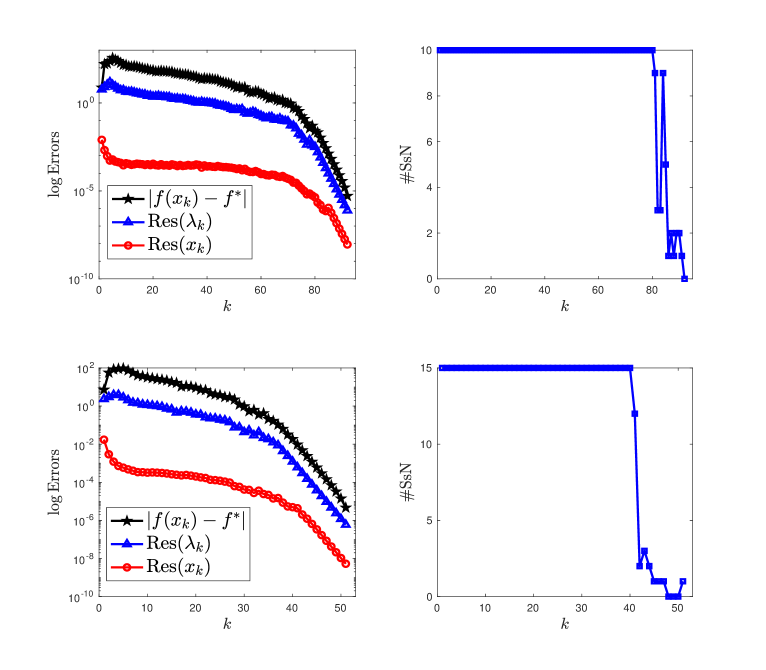
Figure 3: Performance of Algorithm 3 for solving (64) with $m=2000,\,n=5000$ and $\rho=0.0005$. The maximal iteration numbers of the SsN iteration for the top row and the bottom row are $j_{\max}=10$ and $j_{\max}=15$, respectively. The left part plots the decay behavior of the errors and the right part shows the number of SsN iteration in each step.

We consider a more singular case $\rho=0.0005$ and restart the algorithm whenever $\beta_{k}\leqslant 10^{-7}$ and the KKT residual ${\rm Res}(k)$ increases. From Figure 3, we observe that for this extreme case, (i) the total iteration number increases; (ii) in more than half of the total number of iterations, the errors decay slowly and the SsN iteration number attains its maximal value $j_{\max}$ (we set $j_{\max}=10$ for the top row and $j_{\max}=15$ for the bottom row), but after that, fast local linear convergence arises and the number of SsN iterations decreases.

As suggested by the results in Figure 3, a warm-up procedure might improve the performance of the algorithm and we show this in Figure 4, where the initial guess is obtained by running the ALB method 500 times. This works well indeed and the convergence behavior is much better than that in Figure 3.

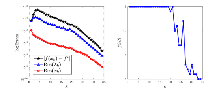
Figure 4: Performance of Algorithm 3 for solving (64) with warm-up procedure. Here, we take $m=2000,\,n=5000$ and $\rho=0.0005$, and the maximal number of the SsN iteration is $j_{\max}=15$. The initial guess is obtained via running the ALB method 500 times.

5.2 Total-variation based image denoising

Given a noised image $g\in L^{2}(\Omega)$ with the domain $\Omega\subset\,{\mathbb{R}}^{2}$, the total variation based denoising model proposed by Rudin, Osher and Fatemi (ROF for short) [68] reads as follows

$$\min_{u}\int_{\Omega}\left\lvert{\nabla u}\right\rvert\,{\rm d}x+\frac{\rho}{2}\left\lVert{u-g}\right\rVert^{2}_{L^{2}(\Omega)},$$ (70)

where $\rho>0$ is the regularization parameter and $\left\lvert{\nabla u}\right\rvert:=\sqrt{|\nabla_{x}u|^{2}+|\nabla_{y}u|^{2}}$.

5.2.1 Discrete formulations

In discrete setting, problem 70 becomes

$$\min_{U\in\,{\mathbb{R}}^{m\times n}}\sum_{i=1}^{m}\sum_{j=1}^{n}\sqrt{|\left(\mathcal{D}(U)\right)_{i,j,1}|^{2}+|\left(\mathcal{D}(U)\right)_{i,j,2}|^{2}}+\frac{\rho}{2}\left\lVert{U-\Xi}\right\rVert^{2}_{F},$$ (71)

where $\Xi\in\,{\mathbb{R}}^{m\times n}$ and $\mathcal{D}:\,{\mathbb{R}}^{m\times n}\to\,{\mathbb{R}}^{m\times n\times 2}$ denotes the discrete gradient operator, i.e.,

$$\left(\mathcal{D}(U)\right)_{i,j,1}:=\left\{\begin{aligned} {}&U_{i+1,j}-U_{i,j}&&\text{if}\,i<m,\\ {}&0&&\text{if}\,i=m,\end{aligned}\right.\quad\text{and}\quad\left(\mathcal{D}(U)\right)_{i,j,2}:=\left\{\begin{aligned} {}&U_{i,j+1}-U_{i,j}&&\text{if}\,j<n,\\ {}&0&&\text{if}\,j=n,\\ \end{aligned}\right.$$

for all $1\leqslant i\leqslant m$ and $1\leqslant j\leqslant n$. Let ${\rm vec}(\times)$ be the vector expanded by the matrix $\times$ by its column. Then rewrite 71 as a composite problem

$$\min_{u\in\,{\mathbb{R}}^{mn}}\,\psi(Au)+\frac{\rho}{2}\left\lVert{u-\xi}\right\rVert^{2},$$ (72)

where $\xi={\rm vec}(\Xi)$ and $A:=\begin{pmatrix}I_{n}\otimes D_{m}\\ D_{n}\otimes I_{m}\\ \end{pmatrix}$, with the difference matrices $D_{m}$ and $D_{n}$ being defined such that $(I_{n}\otimes D_{m}){\rm vec}(U)={\rm vec}(\mathcal{D}(U)_{i,j,1})$ and $(D_{n}\otimes I_{m}){\rm vec}(U)={\rm vec}(\mathcal{D}(U)_{i,j,2})$.

Let $\mathcal{A}=(-A,I)$ and introduce a function $\psi:\,{\mathbb{R}}^{2mn}\to\,{\mathbb{R}}$ by that

$$\psi(\bm{p}):=\sum_{i=1}^{mn}\sqrt{p_{i}^{2}+q_{i}^{2}}\quad\forall\,\bm{p}=\begin{pmatrix}p\\ q\end{pmatrix}\in\,{\mathbb{R}}^{2mn}.$$

Then 72 can be written as the standard form 1:

$$\min_{X=(u,\bm{p})}f(X):=\frac{\rho}{2}\left\lVert{u-\xi}\right\rVert^{2}+\psi(\bm{p})\quad{\rm s.t.}\,\mathcal{A}X=0.$$ (73)

5.2.2 Accelerated primal-dual methods

There are some well-known accelerated primal-dual methods for solving the discrete ROF model 71. Here, we choose two baseline algorithms: the primal-dual hybrid gradient (PDHG) method [16, Algorithm 2] and the accelerated alternating direction method of multipliers (A-ADMM) [82, Algorithm 2]. Ergodic convergence rate $\mathcal{O}(1/k^{2})$ is achieved by those two methods. For completeness, we list them as below.

• PDHG method [16, Algorithm 2]  This method starts from the minimax formulation of 72:

  $$\min_{u\in\,{\mathbb{R}}^{mn}}\max_{\bm{\lambda}\in\,{\mathbb{R}}^{2mn}}\left\langle{Au,\bm{\lambda}}\right\rangle+\frac{\rho}{2}\left\lVert{u-\xi}\right\rVert^{2}-\psi^{*}(\bm{\lambda}),$$ (74)

  where

  $$\bm{\lambda}=\begin{pmatrix}v\\ w\end{pmatrix}\in\,{\mathbb{R}}^{2mn}\quad\text{and}\quad\psi^{*}(\bm{\lambda}):=\left\{\begin{aligned} {}&0&&\text{if }\sqrt{v_{i}^{2}+w_{i}^{2}}\leqslant 1\text{ for all }1\leqslant i\leqslant mn,\\ {}&+\infty&&\text{ else}.\end{aligned}\right.$$

  More precisely, it reads as follows: given $\sigma_{0}=0,\,\bm{\lambda}_{0}\in\,{\mathbb{R}}^{2mn}$ and $u_{-1}=u_{0}\in\,{\mathbb{R}}^{mn}$, do the iteration

  $$\left\{\begin{aligned} {}&\bar{u}_{k}=u_{k}+\sigma_{k}(u_{k}-u_{k-1}),\\ {}&\bm{\lambda}_{k+1}={\bf prox}_{\theta_{k}\psi^{*}}(\bm{\lambda}_{k}+\theta_{k}A\bar{u}_{k}),\\ {}&u_{k+1}=\frac{u_{k}-\tau_{k}A^{\top}\bm{\lambda}_{k+1}}{1+\rho\tau_{k}}+\frac{\rho\tau_{k}\xi}{1+\rho\tau_{k}},\\ {}&\sigma_{k+1}={}1/\sqrt{1+2\rho\tau_{k}},\,\tau_{k+1}=\sigma_{k+1}\tau_{k},\,\theta_{k+1}=\theta_{k}/\sigma_{k+1},\end{aligned}\right.$$ (75)

  where $\tau_{0}\theta_{0}\left\lVert{A}\right\rVert^{2}\leqslant 1$ with $\left\lVert{A}\right\rVert^{2}\leqslant 8$ (cf. [15]). Thanks to Moreau’s identity 52, for all $\theta>0$, we have ${\bf prox}_{\theta\psi^{*}}(\bm{\lambda})=(v\odot\sigma(\bm{\lambda}),w\odot\sigma(\bm{\lambda}))$, where $\sigma(\bm{\lambda}):=1-\tau(v,w)$ with $\tau(v,w)$ being defined by 77.

• A-ADMM [82, Algorithm 2]  Applying this method to problem 73 leads to the iteration: given $\theta\geqslant\left\lVert{A}\right\rVert^{2},\lambda_{0}=0,\,\bm{p}_{0}\in\,{\mathbb{R}}^{2mn}$ and $u_{0}\in\,{\mathbb{R}}^{mn}$, compute

  $$\left\{\begin{aligned} {}&\theta_{k}=\frac{2\theta}{\rho(k+1)},\\ {}&\bm{p}_{k+1}={\bf prox}_{\theta_{k}\psi}(Au_{k}-\theta_{k}\lambda_{k}),\\ {}&u_{k+1}=\left(\rho\theta_{k}I+A^{\top}A\right)^{-1}\left(A^{\top}(\bm{p}_{k+1}+\theta_{k}\lambda_{k})+\rho\theta_{k}\xi\right),\\ {}&\lambda_{k+1}=\lambda_{k}+\frac{1}{\theta_{k}}\left(\bm{p}_{k+1}-Au_{k+1}\right),\end{aligned}\right.$$ (76)

  where ${\bf prox}_{\theta_{k}\psi}(\cdot)$ is defined by 78 and the inverse operation $\left(\rho\theta_{k}I+A^{\top}A\right)^{-1}$ can be realized via fast Fourier transform.

5.2.3 Inexact implicit primal-dual method

We apply our Algorithm 1 to problem 73 and obtain an inexact Im-PD method; see Algorithm 4. For clarity, we provide some details about the proximal calculations. Given $a,b\in\,{\mathbb{R}}$ and $\theta>0$, define $\tau_{\theta}(a,b)\in\,{\mathbb{R}}$ and $\mathcal{T}_{\theta}(a,b)\in\,{\mathbb{R}}^{2\times 2}$ respectively by that

$$\tau_{\theta}(a,b):={} 1-\frac{\theta}{\max\left\{\theta,\sqrt{a^{2}+b^{2}}\right\}},$$

$$\mathcal{T}_{\theta}(a,b):={} \left\{\begin{aligned} {}&\tau_{\theta}(a,b)I+\frac{1-\tau_{\theta}(a,b)}{a^{2}+b^{2}}\begin{pmatrix}a^{2}&ab\\ ab&b^{2}\end{pmatrix}&&\text{ if }\sqrt{a^{2}+b^{2}}\geqslant\theta,\\ {}&O_{2\times 2}&&\text{else}.\end{aligned}\right.$$

If $a,\,b\in\,{\mathbb{R}}^{n}$, then $\tau_{\theta}(a,b)\in\,{\mathbb{R}}^{n}$ can be understood as point wise operation:

$$\tau_{\theta}(a,b):={}{\bf 1}_{n}-\theta{\bf 1}_{n}\oslash\max\{\theta{\bf 1}_{n},\sqrt{a\odot a+b\odot b}\}.$$ (77)

For $\theta=1$, we simply write $\tau_{\theta}(a,b)=\tau(a,b)$.

For $X=(u,\bm{p})\in\,{\mathbb{R}}^{3mn}$ and $\theta>0$, the proximal mapping of $f$ is given by ${\bf prox}_{\theta f}(X)=(\frac{u+\rho\theta\xi}{1+\rho\theta},{\bf prox}_{\theta\psi}(\bm{p}))$, where

$${\bf prox}_{\theta\psi}(\bm{p})=(p\odot\tau_{\theta}(p,q),q\odot\tau_{\theta}(p,q)).$$ (78)

According to [32, Chapter 7], $f$ is strongly semismooth and so is the nonlinear mapping $F_{k}(\cdot)$ defined by 80. Moreover, a direct computation shows that $P_{\theta}(X)\in\partial{\bf prox}_{\theta f}(X)$ where

$$P_{\theta}(X):=\begin{pmatrix}\frac{1}{1+\rho\theta}I&O\\ O&T\\ \end{pmatrix}\quad\text{with}\quad T=\begin{pmatrix}{\rm diag}(\tau_{11})&{\rm diag}(\tau_{12})\\ {\rm diag}(\tau_{21})&{\rm diag}(\tau_{22})\\ \end{pmatrix}.$$ (79)

In 79, $T$ is block diagonal and $\mathcal{T}_{\theta}(p_{i},q_{i})=\begin{pmatrix}(\tau_{11})_{i}&(\tau_{12})_{i}\\ (\tau_{21})_{i}&(\tau_{22})_{i}\\ \end{pmatrix}$ for all $1\leqslant i\leqslant mn$. For $Y=(s,\bm{\lambda})\in\,{\mathbb{R}}^{3mn}$, it is not hard to find that $f^{*}(Y)=\frac{1}{2\rho}\left\lVert{s}\right\rVert^{2}+\left\langle{s,\xi}\right\rangle+\psi^{*}(\bm{\lambda})$, and thus the function 53 becomes

$$\mathcal{F}_{k}(\bm{\lambda})={} \frac{\beta_{k+1}}{2}\left\lVert{\bm{\lambda}}\right\rVert^{2}-\left\langle{Z_{k},\bm{\lambda}}\right\rangle+f^{*}(Y_{k}(\bm{\lambda}))+\frac{1}{2\theta_{k}}\left\lVert{{\bf prox}_{\theta_{k}f}[Y_{k}(\bm{\lambda})]}\right\rVert^{2},$$

where $Z_{k}={}\beta_{k+1}\left(\bm{\lambda}_{k}-\beta_{k}^{-1}\mathcal{A}X_{k}\right)$ and $Y_{k}(\bm{\lambda})=X_{k}-\theta_{k}\mathcal{A}^{\top}\bm{\lambda}$.

As motivated by the first example (cf. Figure 4), in line 3 of Algorithm 4, we consider a warm-up step to provide a reasonable initial guess $(X_{0},\bm{\lambda}_{0})$ and therefore enhance the performance. Besides, in step 13, the linear SPD system has special sparse structure that $T_{k}$ is a $2\times 2$ block matrix with each block being diagonal (see 79) and

$$AA^{\top}=\begin{pmatrix}H_{11}&H_{12}\\ H_{12}^{\top}&H_{22}\end{pmatrix}=\begin{pmatrix}I_{n}\otimes D_{m}D_{m}^{\top}&D_{n}^{\top}\otimes D_{m}\\ D_{m}^{\top}\otimes D_{n}&D_{n}D_{n}^{\top}\otimes I_{m}\\ \end{pmatrix},$$

where $H_{11}$ is block diagonal and both $H_{12}$ and $H_{22}$ are block tridiagonal. Hence, we consider the incomplete Cholesky factorization (cf. [69, Chapter 10]) as a preconditioner and apply preconditioned CG to step 13 to obtain an approximation with relative residual $\leqslant 10^{-8}$.

Algorithm 4 Inexact Im-PD method for the discrete ROF model 73

0:  $\beta_{0}>0,\,\nu=0.2$ and $\delta=0.9$.

1:  Problem setting: $\rho>0$ and $\xi\in\,{\mathbb{R}}^{mn}$.

2:  Tolerances: $\mathtt{KKT\_Tol}=10^{-6}$ and $\mathtt{SsN\_Tol}=10^{-8}$.

3:  Perform a warm-up step to obtain: $X_{0}=(u_{0},\bm{p}_{0})\in\,{\mathbb{R}}^{3mn}$ and $\bm{\lambda}_{0}\in\,{\mathbb{R}}^{2mn}$.

4:  for $k=0,1,\ldots$ do

5:     Choose the step size $\alpha_{k}>0$ and update $\displaystyle\beta_{k+1}=\beta_{k}/(1+\alpha_{k})$.

6:     Set $\displaystyle\theta_{k}={}\alpha_{k}/\beta_{k}$ and $\rho_{k}=1/(1+\rho\theta_{k})$.

7:     Set $\displaystyle Z_{k}={}\beta_{k+1}\left(\bm{\lambda}_{k}-\beta_{k}^{-1}\mathcal{A}X_{k}\right)$.

8:     Solve $\bm{\lambda}_{k+1}$ from the nonlinear equation

$$F_{k}(\bm{\lambda}):=\beta_{k+1}\bm{\lambda}-\mathcal{A}{\bf prox}_{\theta_{k}f}\left(X_{k}-\theta_{k}\mathcal{A}^{\top}\bm{\lambda}\right)-Z_{k}=0$$ (80)

via the following SsN iteration with the initial guess $\bm{\lambda}=\bm{\lambda}_{k}$:

9:     while $\left\lVert{F_{k}(\bm{\lambda})}\right\rVert>\mathtt{SsN\_Tol}$ do {SsN iteration}

10:        Compute $Y_{k}=X_{k}-\theta_{k}\mathcal{A}^{\top}\bm{\lambda}$.

11:        Find $P_{k}(Y_{k})=\begin{pmatrix}\rho_{k}I&O\\ O&T_{k}\end{pmatrix}\in\partial{\bf prox}_{\theta_{k}f}(Y_{k})$ via 79.

12:        Compute $JF_{k}(\bm{\lambda})=\beta_{k+1}I+\theta_{k}T_{k}+\rho_{k}\theta_{k}AA^{\top}$.

13:        Solve $JF_{k}(\bm{\lambda})\bm{d}=-F_{k}(\bm{\lambda})$ approximately via preconditioned CG.

14:        Find the smallest integer $r\in\mathbb{N}_{+}$ such that $\mathcal{F}_{k}(\bm{\lambda}+\delta^{r}\bm{d})\leqslant\mathcal{F}_{k}(\bm{\lambda})+\nu\delta^{r}\left\langle{F_{k}(\bm{\lambda}),\bm{d}}\right\rangle$.

15:        Update $\bm{\lambda}=\bm{\lambda}+\delta^{r}\bm{d}$.

16:     end while

17:     Update $\bm{\lambda}_{k+1}=\bm{\lambda}$ and $X_{k+1}={\bf prox}_{\theta_{k}f}\left(X_{k}-\theta_{k}\mathcal{A}^{\top}\bm{\lambda}_{k+1}\right)$.

18:     if ${\rm Res}(k)\leqslant\mathtt{KKT\_Tol}$ then

19:        break

20:     end if

21:  end for

5.2.4 Numerical results

We adopt four benchmark images from the literature: $\mathtt{barb}$, $\mathtt{boat}$, $\mathtt{cameraman}$ and $\mathtt{lena}$. These images are noised with standard normal distribution. Note that both 74 and 73 admit the same optimality condition

$$\left\{\begin{aligned} 0={}&\rho(u^{*}-\xi)-A^{\top}\bm{\lambda}^{*}\\ 0\in{}&\bm{\lambda}^{*}+\partial\psi(\bm{p}^{*})\\ 0={}&\bm{p}^{*}-Au^{*}\\ \end{aligned}\right.\quad\Longleftrightarrow\quad\left\{\begin{aligned} 0={}&\rho(u^{*}-\xi)-A^{\top}\bm{\lambda}^{*}\\ 0={}&\bm{p}^{*}-{\bf prox}_{\psi}(\bm{p}^{*}-\bm{\lambda}^{*})\\ 0={}&\bm{p}^{*}-Au^{*}=0\end{aligned}\right..$$

Hence, we consider the stopping criterion:

$${\rm Res}(k):=\max\left\{{\rm Res}(u_{k}),\,{\rm Res}(\bm{p}_{k}),\,{\rm Res}(\bm{\lambda}_{k})\right\}\leqslant\mathtt{KKT\_Tol}=10^{-6},$$ (81)

where the relative KKT residuals are defined by

$$\small{\rm Res}(u_{k}):=\frac{\left\lVert{\rho(u_{k}-\xi)-A^{\top}\bm{\lambda}_{k}}\right\rVert}{1+\left\lVert{\xi}\right\rVert},\,{\rm Res}(\bm{p}_{k}):=\frac{\left\lVert{\bm{p}_{k}-{\bf prox}_{\psi}(\bm{p}_{k}-\bm{\lambda}_{k})}\right\rVert}{1+\left\lVert{\bm{p}_{k}}\right\rVert}\,\text{and}\,{\rm Res}(\bm{\lambda}_{k}):=\frac{\left\lVert{\bm{p}_{k}-Au_{k}}\right\rVert}{1+\left\lVert{\bm{p}_{k}}\right\rVert}.$$

For all methods, the maximal iteration number is $k_{\max}=1e5$. For inexact Im-PD (i.e. Algorithm 4), we run the A-ADMM with 50 steps to obtain an initial guess $(u_{0},\bm{p}_{0},\bm{\lambda}_{0})$ with $\max\left\{{\rm Res}(u_{0}),\,{\rm Res}(\bm{p}_{0}),\,{\rm Res}(\bm{\lambda}_{0})\right\}\approx 10^{-2}$ and choose the step size $\alpha_{k}=1+\sigma$ where $\sigma$ obeys the uniform distribution on $[0,1]$. Then by Lemma 3.1, we have the linear rate $\varrho^{k}$ with $\varrho=\mathbb{E}[\frac{1}{1+\alpha_{k}}]=\int_{0}^{1}\frac{1}{2+\sigma}\,{\rm d}\sigma=\ln 3/2$ and the required iteration number for 81 is about $k^{*}=-4\ln 10/\ln\varrho\approx 10$.

Table 2: Performances of Algorithm 4, PDHG 75 and A-ADMM 76 for solving 71.

						Inexact Im-PD (Algorithm 4)					A-ADMM 76			PDHG 75
		$m=n$		$\rho$		its	SsN	warm-up(sec)	time(sec)		its	time(sec)		its	Res$(k_{\max})$	time(sec)
$\mathtt{barb}$		512		50		10	182	47.11	830.53		1572	1497.40		$10^{5}$	5.15e-06	5169.55
				150		10	141	41.76	568.34		3445	3192.33			3.59e-06	5213.23
$\mathtt{boat}$		512		40		9	84	54.53	457.05		1300	1145.84		$10^{5}$	5.49e-06	5228.70
				180		10	141	44.34	611.90		3866	3316.70			3.42e-06	5223.88
$\mathtt{cameraman}$		256		20		7	52	8.48	78.91		724	124.58		$10^{5}$	7.77e-06	1299.35
				100		10	81	8.36	70.26		2575	448.94			4.10e-06	1262.76
$\mathtt{lena}$		256		50		9	111	8.55	117.86		1554	288.23		$10^{5}$	5.29e-06	1229.09
				200		11	157	8.47	158.41		4099	758.60			3.55e-06	1210.58

Computational results are summarized in Table 2, including the number of iterations (its) and running time (time). For Inexact Im-PD, we also report the total number of SsN iterations (SsN) and the time used for initialization (warm-up). For all cases, PDHG has not achieved the tolerance 81 within the maximal iteration number $k_{\max}=10^{5}$, and we also record the KKT residual Res$(k_{\max})$ at the last iterate. As we can see, Algorithm 4 outperforms much better than other two methods and the total iteration number is almost $10$, as expected above. Particularly, we observe that A-ADMM is more efficient than PDHG.

Moreover, in Figure 5, we plot the averaged PCG iteration number of Algorithm 4 for all cases. Similar as before (cf. Figure 2), it increases along with the iteration. Therefore, this deserves further study for more robust and efficient linear solvers such as algebraic multilevel methods [50, 83].

6 Concluding Remarks

In this work, we introduce a novel dynamical system, called primal-dual flow, for solving affine constrained convex optimization. The current model is a modification of the standard saddle-point dynamics. In continuous level, exponential decay of a tailored Lyapunov function is established. Then, in discrete level, primal-dual type algorithms are obtained from proper time discretizations of the presented primal-dual flow and nonergodic convergence rates are established via a unified discrete Lyapunov function.

The proposed methods adopt dynamically changing parameters and the subproblem with respect to the multiplier is solved by the semi-smooth Newton iteration. This can be quite efficient provided that the problem has nice properties such as semi-smoothness and sparsity, as showed by numerical results of the $l_{1}$-$l_{2}$ problem and the total-variation based denoising model.

To the end, we list several ongoing works. First, well-posedness (existence and uniqueness) of the primal-dual flow system 26a is an interesting topic. Also, the exponential decay property 16 and weak convergence of the trajectory under general nonsmooth setting deserves future investigations. Besides, rigorous convergence rate analysis with inexact computation and restart technique requires further attentions.

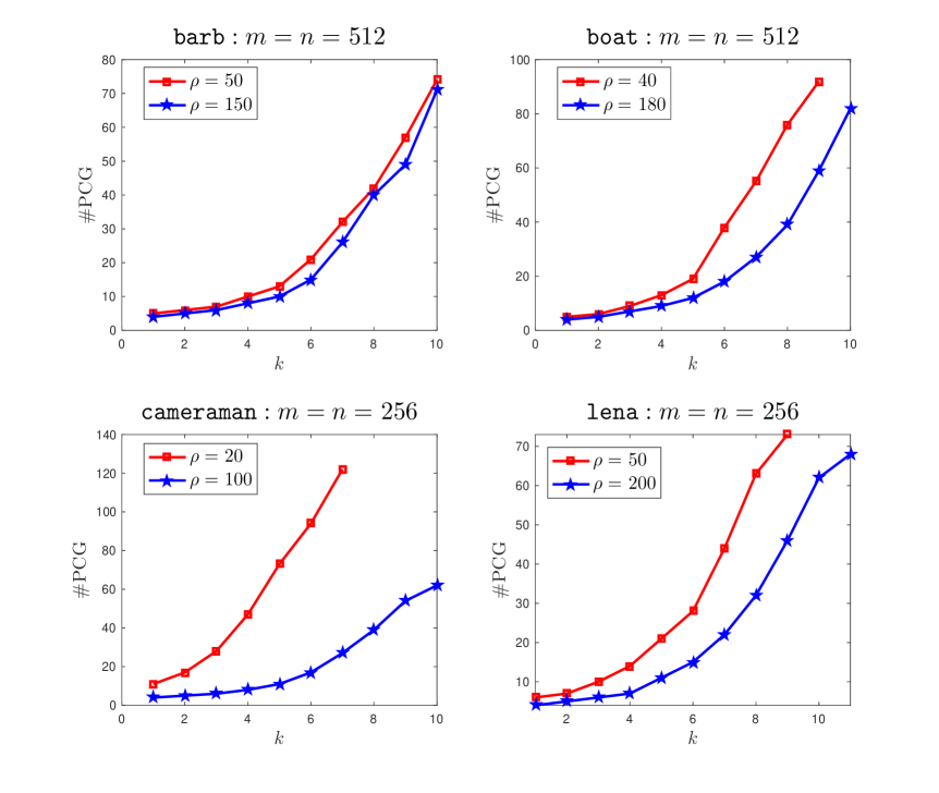
Figure 5: Averaged PCG iterations of Algorithm 4 for solving 71 with different noised input images and regularization parameters.

Appendix A An Over-Relaxation Perspective

In Section 2.2, we introduced our primal-dual flow by adding the extra term $x^{\prime}$, which is motivated from the disappointing estimate in Lemma 2.1 and leads to the desired exponential decay, and later in Section 2.3, we provided an equilibrium illustration to show further the positive effects of this correction.

To better understand the modification from the saddle-point system 4 to our new model 15a, in this appendix, by using the PPA-like interpretation [44], we give a discrete over-relaxation perspective, which indicates somewhat subtle connection with the hidden symmetrization from the Arrow–Hurwicz algorithm [89] to the PDHG method [16]. We hope this provides a more reasonably intrinsic explanation.

The Arrow–Hurwicz algorithm can be applied to 1 and reads as

$$\left\{\begin{aligned} x_{k+1}={}&\mathop{{\mathop{{\rm argmin}}\,}}_{x\in\,{\mathbb{R}}^{n}}\left\{\mathcal{L}(x,\lambda_{k})+\frac{1}{2r}\left\lVert{x-x_{k}}\right\rVert^{2}\right\},\\ \lambda_{k+1}={}&\mathop{{\mathop{{\rm argmax}}\,}}_{\lambda\in\,{\mathbb{R}}^{m}}\left\{\mathcal{L}(x_{k+1},\lambda)-\frac{1}{2\tau}\left\lVert{\lambda-\lambda_{k}}\right\rVert^{2}\right\},\end{aligned}\right.$$ (82)

with step sizes $r,\,\tau>0$. It also corresponds to a semi-implicit discretization for 4:

$$\left\{\begin{aligned} \frac{x_{k+1}-x_{k}}{r}\in{}&-\partial_{x}\mathcal{L}(x_{k+1},\lambda_{k}),\\ \frac{\lambda_{k+1}-\lambda_{k}}{\tau}={}&\nabla_{\lambda}\mathcal{L}(x_{k+1},\lambda_{k+1}).\end{aligned}\right.$$ (83)

Following [44] and [13, Chapter 8], we use the PPA-like interpretation to demonstrate the lack of symmetry of the Arrow–Hurwicz algorithm. Introduce

$$\small Z=\begin{pmatrix}x\\ \lambda\end{pmatrix},\quad M(Z)=\begin{pmatrix}\partial f(x)+A^{\top}\lambda\\ b-Ax\end{pmatrix}\quad\text{and}\quad Q=\begin{pmatrix}I/r&-A^{\top}\\ O&I/\tau\end{pmatrix},$$

where the maximally monotone operator $M$ has been defined in 22. We then have the variational inequality characterization for 82 (or 83):

$$\left\langle{Q(Z_{k+1}-Z_{k})+M(Z_{k+1}),Z-Z_{k+1}}\right\rangle\geqslant 0\quad\forall\,Z\in\,{\mathbb{R}}^{n+m}.$$

Taking $Z=Z^{*}\in\Omega^{*}$ and utilizing the fact: $0\in M(Z^{*})$, we find that

$$\frac{1}{2}\left\lVert{Z_{k+1}-Z^{*}}\right\rVert_{Q}^{2}-\frac{1}{2}\left\lVert{Z_{k}-Z^{*}}\right\rVert_{Q}^{2}$$ (84)

$$={} \left\langle{Q(Z_{k+1}-Z_{k}),Z_{k+1}-Z^{*}}\right\rangle-\frac{1}{2}\left\lVert{Z_{k+1}-Z_{k}}\right\rVert_{Q}^{2}+\frac{1}{2}\big{\langle}(Q^{\top}-Q)(Z_{k+1}-Z^{*}),Z_{k}-Z^{*}\big{\rangle}$$

$$\leqslant{} \underbrace{-\left\langle{M(Z_{k+1}),Z_{k+1}-Z^{*}}\right\rangle}_{\leqslant 0}-\frac{1}{2}\left\lVert{Z_{k+1}-Z_{k}}\right\rVert_{Q}^{2}+\frac{1}{2}\big{\langle}(Q^{\top}-Q)(Z_{k+1}-Z^{*}),Z_{k}-Z^{*}\big{\rangle}$$

$$\leqslant{}{} -\frac{1}{2}\left\lVert{Z_{k+1}-Z_{k}}\right\rVert_{Q}^{2}+\frac{1}{2}\big{\langle}\underbrace{(Q^{\top}-Q)}_{\neq 0}(Z_{k+1}-Z^{*}),Z_{k}-Z^{*}\big{\rangle}.$$

As $Q$ is not symmetric, the last term makes it hard to obtain the descent estimate, and what’s even worse, the scheme (82) is not necessarily convergent [42].

The PDHG method of Chambolle and Pock introduces a parameter $\theta\in[0,1]$ and becomes

$$\left\{\begin{aligned} x_{k+1}={}&\mathop{{\mathop{{\rm argmin}}\,}}_{x\in\,{\mathbb{R}}^{n}}\left\{\mathcal{L}(x,\lambda_{k})+\frac{1}{2r}\left\lVert{x-x_{k}}\right\rVert^{2}\right\},\\ \lambda_{k+1}={}&\mathop{{\mathop{{\rm argmax}}\,}}_{\lambda\in\,{\mathbb{R}}^{m}}\left\{\mathcal{L}(x_{k+1}+\theta(x_{k+1}-x_{k}),\lambda)-\frac{1}{2\tau}\left\lVert{\lambda-\lambda_{k}}\right\rVert^{2}\right\},\end{aligned}\right.$$ (85)

which is also equivalent to

$$\left\{\begin{aligned} \frac{x_{k+1}-x_{k}}{r}\in{}&-\partial_{x}\mathcal{L}(x_{k+1},\lambda_{k}),\\ \frac{\lambda_{k+1}-\lambda_{k}}{\tau}={}&\nabla_{\lambda}\mathcal{L}(x_{k+1}+\theta(x_{k+1}-x_{k}),\lambda_{k+1}).\end{aligned}\right.$$ (86)

Comparing this with the previous discretization (83), we observe the additional extrapolation term $x_{k+1}-x_{k}$. For the case $\theta=1$, we have ergodic convergence rate $\mathcal{O}(1/k)$ under the condition $r\tau\left\lVert{A}\right\rVert^{2}<1$. Moreover, applying the above PPA-like framework to the PDHG method (with $\theta=1$), one observes that the estimate 84 is now improved to

$$\frac{1}{2}\left\lVert{Z_{k+1}-Z^{*}}\right\rVert_{\widehat{Q}}^{2}-\frac{1}{2}\left\lVert{Z_{k}-Z^{*}}\right\rVert_{\widehat{Q}}^{2}\leqslant{}{}-\frac{1}{2}\left\lVert{Z_{k+1}-Z_{k}}\right\rVert_{\widehat{Q}}^{2}\quad\text{with}\quad{\widehat{Q}}=\begin{pmatrix}I/r&-A^{\top}\\ -A&I/\tau\end{pmatrix},$$

where $\widehat{Q}$ is a symmetrization of $Q$, due to the over-relaxation $x_{k+1}-x_{k}$.

Surprisingly, instead of the original saddle-point system 4, the PDHG method 85 is more likely a time discretization (cf. 86) for the modified model

$$\left\{\begin{aligned} {}&x^{\prime}=-\nabla_{x}\mathcal{L}(x,\lambda),\\ {}&\lambda^{\prime}={}\nabla_{\lambda}\mathcal{L}(x+x^{\prime},\lambda),\end{aligned}\right.$$

which differs from our primal-dual flow 15a only in the time scaling parameters. In conclusion, the extra derivative $x^{\prime}$ in $\nabla_{\lambda}\mathcal{L}(x+x^{\prime},\lambda)$ corresponds to discrete over-relaxation $x_{k+1}-x_{k}$ in PDHG, which possibly brings hidden symmetrization.

References

• [1] T. Aspelmeier, C. Charitha, and D. R. Luke. Local linear convergence of the ADMM/Douglas–Rachford algorithms without strong convexity and application to statistical imaging. SIAM J. Imaging Sci., 9(2):842–868, 2016.
• [2] H. Attouch, Z. Chbani, J. Peypouquet, and P. Redont. Fast convergence of inertial dynamics and algorithms with asymptotic vanishing viscosity. Math. Program. Series B, 168(1-2):123–175, 2018.
• [3] H. Attouch, X. Goudou, and P. Redont. The heavy ball with friction method, I. The continuous dynamical system: Global exploration of the local minima of a real-valued function by asymptotic analysis of a dissipative dynamical system. Commun. Contemp. Math., 2(1):1–34, 2000.
• [4] H. Attouch, J. Peypouquet, and P. Redont. Fast convex optimization via inertial dynamics with Hessian driven damping. J. Differ. Equ., 261(10), 2016.
• [5] A. Beck. First-Order Methods in Optimization, volume 1 of MOS–SIAM Series on Optimization. Society for Industrial and Applied Mathematics and the Mathematical Optimization Society, 2017.
• [6] A. Beck and M. Teboulle. A fast iterative shrinkage-thresholding algorithm for linear inverse problems. SIAM J. Imaging Sci., 2(1):183–202, 2009.
• [7] A. Beck and M. Teboulle. Gradient-based algorithms with applications to signal-recovery problems. In D. Palomar and Y. Eldar, editors, Convex Optimization in Signal Processing and Communications, pages 42–88. Cambridge University Press, Cambridge, 2009.
• [8] D. Bertsekas. Constrained Optimization and Lagrange Multiplier Methods. Academic Press, New York, 2014.
• [9] S. Bonettini and V. Ruggiero. On the convergence of primal–dual hybrid gradient algorithms for total variation image restoration. J.Math. Imaging Vis., 44(3):236–253, 2012.
• [10] S. Boyd, N. Parikh, E. Chu, and J. Peleato, B.and Eckstein. Distributed optimization and statistical learning via the alternating direction method of multipliers. Found. Trends Mach. Learn., 3(1):1–122, 2010.
• [11] H. Brézis. Operateurs Maximaux Monotones: Et Semi-Groupes De Contractions Dans Les Espaces De Hilbert. North-Holland Publishing Co., North-Holland Mathematics Studies, No. 5. Notas de Matemática (50), 1973.
• [12] J.-F. Cai, S. Osher, and Z. Shen. Linearized Bregman iterations for compressed sensing. Mathematics of Computation, 78(267):1515–1536, 2009.
• [13] C. Clason and T. Valkonen. Nonsmooth Analysis and Optimization. https://arxiv.org/abs/2001.00216, 2020.
• [14] E. Candés and M. Wakin. An introduction to compressive sampling. IEEE Signal Process. Mag., (21):21–30, 2008.
• [15] A. Chambolle. An algorithm for total variation minimization and applications. Journal of Mathematical Imaging and Vision, 20(1/2):89–97, 2004.
• [16] A. Chambolle and T. Pock. A first-order primal-dual algorithm for convex problems with applications to imaging. J.Math. Imaging Vis., 40(1):120–145, 2011.
• [17] A. Chambolle and T. Pock. An introduction to continuous optimization for imaging. Acta Numerica, 25:161–319, 2016.
• [18] A. Chambolle and T. Pock. On the ergodic convergence rates of a first-order primal–dual algorithm. Math. Program., 159(1-2):253–287, 2016.
• [19] L. Chen and H. Luo. A unified convergence analysis of first order convex optimization methods via strong Lyapunov functions. arXiv: 2108.00132, 2021.
• [20] L. Chen and H. Luo. First order optimization methods based on Hessian-driven Nesterov accelerated gradient flow. arXiv: 1912.09276, 2019.
• [21] S. Chen, D. Donoho, and M. Saunders. Atomic decomposition by basis pursuit. SIAM J. Sci. Comput., (20):33–61, 1999.
• [22] A. Cherukuri, B. Gharesifard, and J. Cortés. Saddle-point dynamics: conditions for asymptotic stability of saddle points. SIAM J. Control Optim., 55(1):486–511, 2017.
• [23] A. Cherukuri, E. Mallada, and J. Cortés. Asymptotic convergence of constrained primal-dual dynamics. Syst. Control Lett., 87:10–15, 2016.
• [24] F. Clarke. Optimization and Nonsmooth Analysis. Number 5 in Classics in Applied Mathematics. Society for Industrial and Applied Mathematics, 1987.
• [25] D. Davis and W. Yin. Faster convergence rates of relaxed Peaceman-Rachford and ADMM under regularity assumptions. arXiv:1407.5210, 2015.
• [26] W. Deng and W. Yin. On the global and linear convergence of the generalized alternating direction method of multipliers. J. Sci. Comput., 66(3):889–916, 2016.
• [27] J. Dennis and R. Schnabel. Numerical Methods for Unconstrained Optimization and Nonlinear Equations. Number 16 in Classics in applied mathematics. Society for Industrial and Applied Mathematics, Philadelphia, 1996.
• [28] B. Djafari-Rouhani and H. Khatibzadeh. Nonlinear Evolution and Difference Equations of Monotone Type in Hilbert Spaces. CRC Press, Boca Raton, 1st edition, 2019.
• [29] J. Douglas and H. H. Rachford. On the numerical solution of heat conduction problems in two and three space variables. Trans. Amer. Math. Soc., 82:421–439, 1956.
• [30] J. Eckstein. Augmented Lagrangian and alternating direction methods for convex optimization: a tutorial and some illustrative computational results. Technical report, Rutgers University, 2012.
• [31] E. Esser, X. Zhang, and T. F. Chan. A general framework for a class of first order primal-dual algorithms for convex optimization in imaging science. SIAM J. Imaging Sci., 3(4):1015–1046, 2010.
• [32] F. Facchinei and J. Pang. Finite-Dimensional Variational Inequalities and Complementarity Problems, vol 2. Springer, New York, 2006.
• [33] D. Feijer and F. Paganini. Stability of primal-dual gradient dynamics and applications to network optimization. Automatica, 46:1974–1981, 2010.
• [34] G. Franca, D. Robinson, and R. Vidal. ADMM and accelerated ADMM as continuous dynamical systems. 35th Int. Conf. Mach. Learn. ICML 2018, 4(4):2528–2536, 2018.
• [35] M. Fortin and R. Glowinski. On decomposition-coordination methods using an augmented Lagrangian. In Studies in Mathematics and Its Applications, volume 15 of Augmented Lagrangian Methods: Applications to the Numerical Solution of Boundary–Value Problems. North-Holland Publishing, Amsterdam, 1983.
• [36] D. Gabay and B. Mercier. A dual algorithm for the solution of nonlinear variational problems via finite element approximation. Computers & Mathematics with Applications, 2(1):17–40, 1976.
• [37] P. Giselsson and S. Boyd. Linear convergence and metric selection for Douglas–Rachford splitting and ADMM. IEEE Trans. Automat. Contr., 62(2):532–544, 2017.
• [38] J. Han and D. Sun. Newton and quasi-Newton methods for normal maps with polyhedral sets. J. Optim. Theory Appl., 94(3):659–676, 1997.
• [39] D. Han, D. Sun, and L. Zhang. Linear rate convergence of the alternating direction method of multipliers for convex composite quadratic and semi-definite programming. arXiv:1508.02134, 2015.
• [40] A. Haraux. Systèmes dynamiques dissipatifs et applications. Recherches en Mathématiques Appliquées [Research in Applied Mathematics], vol 17. Masson, Paris, 1991.
• [41] X. He, R. Hu, and Y. Fang. Convergence rates of inertial primal-dual dynamical methods for separable convex optimization problems. arXiv:2007.12428, 2020.
• [42] B. He, F. Ma, and X. Yuan. An algorithmic framework of generalized primal–dual hybrid gradient methods for saddle point problems. J Math Imaging Vis, 58:279–293, 2017.
• [43] B. He, Y. You, and X. Yuan. On the convergence of primal-dual hybrid gradient algorithm. SIAM J. Imaging Sci., 7(4):2526–2537, 2014.
• [44] B. He and X. Yuan. Convergence analysis of primal-dual algorithms for a saddle-point problem: from contraction perspective. SIAM J. Imaging Sci., 5(1):119–149, 2012.
• [45] B. Huang, S. Ma, and D. Goldfarb. Accelerated linearized Bregman method. J. Sci. Comput., 54:428–453, 2013.
• [46] F. Jiang, X. Cai, Z. Wu, and D. Han. Approximate first-order primal-dual algorithms for saddle point problems. Math. Comp., 90(329):1227–1262, 2021.
• [47] M. Kang, M. Kang, and M. Jung. Inexact accelerated augmented Lagrangian methods. Comput. Optim. Appl., 62(2):373–404, 2015.
• [48] M. Kang, S. Yun, H. Woo, and M. Kang. Accelerated Bregman method for linearly constrained $\ell_{1}$-$\ell_{2}$ minimization. J. Sci. Comput., 56(3):515–534, 2013.
• [49] G. Lan and R. Monteiro. Iteration-complexity of first-order penalty methods for convex programming. Math. Program., 138(1-2):115–139, 2013.
• [50] Y.-J. Lee, J. Wu, J. Xu, and L. Zikatanov. Robust subspace correction methods for nearly singular systems. Mathematical Models and Methods in Applied Sciences, 17(11):1937–1963, 2007.
• [51] D. Li, X.and Sun and K. Toh. On the efficient computation of a generalized Jacobian of the projector over the Birkhoff polytope. Math. Program., 179(1-2):419–446, 2020.
• [52] H. Li, C. Fang, and Z. Lin. Convergence rates analysis of the quadratic penalty method and its applications to decentralized distributed optimization. arXiv:1711.10802, 2017.
• [53] X. Li, D. Sun, and K. Toh. An asymptotically superlinearly convergent semismooth Newton augmented Lagrangian method for linear programming. SIAM J. Optim., 30(3):2410–2440, 2020.
• [54] T. Lin and M. I. Jordan. A control-theoretic perspective on optimal high-order optimization. arXiv:1912.07168, 2019.
• [55] Y. Liu, X. Yuan, S. Zeng, and J. Zhang. Partial error bound conditions and the linear convergence rate of the alternating direction method of multipliers. SIAM J. Numer. Anal., 56(4):2095–2123, 2018.
• [56] H. Lu. An ${O}(s^{r})$-resolution ODE framework for discrete-time optimization algorithms and applications to convex-concave saddle-point problems. arXiv:2001.08826, 2020.
• [57] H. Luo. Accelerated differential inclusion for convex optimization. Optimization, https://doi.org/10.1080/02331934.2021.2002327, 2021.
• [58] H. Luo and L. Chen. From differential equation solvers to accelerated first-order methods for convex optimization. Math. Program., https://doi.org/10.1007/s10107-021-01713-3, 2021.
• [59] Y. Nesterov. Gradient methods for minimizing composite functions. Math. Program. Series B, 140(1):125–161, 2013.
• [60] D. Niu, C. Wang, P. Tang, Q. Wang, and E. Song. A sparse semismooth Newton based augmented Lagrangian method for large-scale support vector machines. arXiv:1910.01312, 2019.
• [61] D. O’Connor and L. Vandenberghe. On the equivalence of the primal-dual hybrid gradient method and Douglas–Rachford splitting. Math. Program., https://doi.org/10.1007/s10107-018-1321-1,
• [62] S. Osher, M. Burger, D. Goldfarb, J. Xu, and W. Yin. An iterative regularization method for total variation-based image restoration. SIAM J. Multiscale Model. Simul., 4:460–489, 2019.
• [63] N. Parikh and S. Boyd. Proximal algorithms. Foundations and Trends® in Optimization, 1(3):127–239, 2014.
• [64] T. Pock, D. Cremers, H. Bischof, and A. Chambolle. An algorithm for minimizing the Mumford-Shah functional. In 2009 IEEE 12th International Conference on Computer Vision, pages 1133–1140, Kyoto, 2009. IEEE.
• [65] D. W. Peaceman and H. H. Rachford. The numerical solution of parabolic and elliptic differential equations. Journal of the Society for Industrial and Applied Mathematics, 3(1):28–41, 1955.
• [66] L. Qi. Convergence analysis of some algorithms for solving nonsmooth equations. Math. Oper. Res., 18(1):227–244, 1993.
• [67] L. Qi and J. Sun. A nonsmooth version of Newton’s method. Math. Program., 58(1-3):353–367, 1993.
• [68] L. Rudin, S. Osher, and E. Fatemi. Nonlinear total variation based noise removal algorithms. Phys.D Nonlinear Phenom., 60(1–4):259–268, 1992.
• [69] Y. Saad. Iterative Methods for Sparse Linear Systems, 2nd. Society for Industrial and Applied Mathematics, USA, 2003.
• [70] S. Sabach and M. Teboulle. Faster Lagrangian-based methods in convex optimization. arXiv:2010.14314, 2020.
• [71] W. Su, S. Boyd, and E. Candès. A differential equation for modeling Nesterov’s accelerated gradient method: theory and insights. J. Mach. Learn. Res., 17:1–43, 2016.
• [72] M. Tao and X. Yuan. Accelerated Uzawa methods for convex optimization. Math. Comp., 86(306):1821–1845, 2016.
• [73] Q. Tran-Dinh. A unified convergence rate analysis of the accelerated smoothed gap reduction algorithm. Optimization Letters, https://doi.org/10.1007/s11590-021-01775-4, 2021.
• [74] Q. Tran-Dinh. Proximal alternating penalty algorithms for nonsmooth constrained convex optimization. Comput. Optim. Appl., 72(1):1–43, 2019.
• [75] Q. Tran-Dinh and V. Cevher. Constrained convex minimization via model-based excessive gap. In In Proc. the Neural Information Processing Systems (NIPS), volume 27, pages 721–729, Montreal, Canada, 2014.
• [76] Q. Tran-Dinh, O. Fercoq, and V. Cevher. A smooth primal-dual optimization framework for nonsmooth composite convex minimization. SIAM J. Optim., 28(1):96–134, 2018.
• [77] Q. Tran-Dinh and Y. Zhu. Augmented Lagrangian-based decomposition methods with non-ergodic optimal rates. arXiv:1806.05280, 2018.
• [78] Q. Tran-Dinh and Y. Zhu. Non-stationary first-order primal-dual algorithms with faster convergence rates. SIAM J. Optim., 30(4):2866–2896, 2020.
• [79] T. Valkonen. Inertial, corrected, primal-dual proximal splitting. SIAM J. Optim., 30(2):1391–1420, 2020.
• [80] A. C. Wilson, B. Recht, and M. I. Jordan. A Lyapunov analysis of accelerated methods in optimization. J. Mach. Learn. Res., 22:1–34, 2021.
• [81] A. Wibisono, A. Wilson, and M. Jordan. A variational perspective on accelerated methods in optimization. Proc. Nati. Acad. Sci., 113(47):E7351–E7358, 2016.
• [82] Y. Xu. Accelerated first-order primal-dual proximal methods for linearly constrained composite convex programming. SIAM J. Optim., 27(3):1459–1484, 2017.
• [83] J. Xu and L. Zikatanov. Algebraic multigrid methods. Acta Numerica, 26:591–721, 2017.
• [84] W. H. Yang and D. Han. Linear convergence of the alternating direction method of multipliers for a class of convex optimization problems. SIAM J. Numer. Anal., 54(2):625–640, 2016.
• [85] M. Yan and W. Yin. Self equivalence of the alternating direction method of multipliers. arXiv:1407.7400, 2015.
• [86] W. Yin. Analysis and generalizations of the linearized Bregman method. SIAM Journal on Imaging Sciences, 3(4):856–877, 2010.
• [87] X. Yuan, S. Zeng, and J. Zhang. Discerning the linear convergence of ADMM for structured convex optimization through the lens of variational analysis. J. Mach. Learn. Res., 21:1–74, 2020.
• [88] X. Zeng, J. Lei, and J. Chen. Dynamical primal-dual accelerated method with applications to network optimization. arXiv:1912.03690, pages 1–22, 2019.
• [89] M. Zhu and T. Chan. An efficient primal-dual hybrid gradient algorithm for total variation image restoration. Technical report CAM Report 08-34, UCLA, Los Angeles, CA, USA, 2008.