A learning rule balancing energy consumption and information maximization in a feed-forward neuronal network

Abstract

Information measures are often used to assess the efficacy of neural networks, and learning rules can be derived through optimization procedures on such measures. In biological neural networks, computation is restricted by the amount of available resources. Considering energy restrictions, it is thus reasonable to balance information processing efficacy with energy consumption. Here, we studied networks of non-linear Hawkes neurons and assessed the information flow through these networks using mutual information. We then applied gradient descent for a combination of mutual information and energetic costs to obtain a learning rule. Through this procedure, we obtained a rule containing a sliding threshold, similar to the Bienenstock-Cooper-Munro rule. The rule contains terms local in time and in space plus one global variable common to the whole network. The rule thus belongs to so-called three-factor rules and the global variable could be related to a number of biological processes. In neural networks using this learning rule, frequent inputs get mapped onto low energy orbits of the network while rare inputs aren’t learned.

¹Département de Physique Nucléaire et Corpusculaire (DPNC), University of Geneva, Geneva, Switzerland

²CERN, Geneva, Switzerland

e-mail: dmytro.grytskyy@etu.unige.ch or renaud.jolivet@unige.ch

Keywords

Mutual information; energy consumption; plastic networks; non-linear Poisson neurons; three-factor rules; noise

1 Introduction

It is typically assumed that neural networks perform some form of information processing. It is thus a natural idea to apply information theory to assess the efficacy of those networks. Various mutually related information measures have been used in this context. For instance, Kramers-Rao relation and Fisher information are used in reference [5] to obtain an upper limit for information inference, and to relate it to the mutual information between a network’s inputs and outputs in the limit of a large number of neurons. The authors then search for the form of a neuron’s non-linear transmission function optimizing this mutual information measure. In reference [25], the authors similarly search for the optimal form of neuronal non-linearity using the Kullback-Leibler divergence. It is also natural to think of synaptic plasticity induced by neuronal activity as geared towards increasing the performance of information inference. In particular, it is possible to derive learning rules converting neuronal activity in synaptic changes as an optimization procedure of some information metric. In reference [39] for instance, Fisher information is applied to link the refractory period after a spike has been elicited to the shape of the Spike-Timing Dependent Plasticity (STDP) learning window. Nessler and colleagues [24] have also obtained learning rules approximating expectation maximization of the likelihood measure between inputs generated by hidden causes and inputs reconstructed from neurons’ outputs. Reference [26] further generalizes this approach for learning of sequences of inputs in time. In both works, the authors additionally exploit fast global inhibition to achieve a winner takes all regime. A likelihood measure expressed with Kullback-Leibler divergence is also applied in [4] to derive learning rules in an expectation maximization manner for a recurrent network learning a set of sequences. In [29], Linsker formulated an infomax principle, proposing maximization of information about the presented input in the network’s output measured by mutual information, as a goal for network parameters fitting. This concept is applied in [30] for a feed-forward architecture with linear neurons and noisy input, generalized in [1] for non-linear neurons without noise, and applied in [31] for recurrent networks of non-linear neurons solving the task of independent component analysis. In [37], mutual information is used to formulate a general form for plasticity rules and applied to the Hodgkin-Huxley model. Finally, in [8], learning rules optimizing mutual information between neurons’ inputs and outputs are derived in the approximation of rare appearance of inputs in a noisy background.

Theoretically, networks can learn an arbitrary complex structure of external inputs. In biological neural networks however, operational and computational capacities are not arbitrarily large, but are restricted by the amount of available resources. Energy is one of these resources [12, 9]. In the mammalian brain, energy is mostly spent at synapses, to power post-synaptic potentials, and to a lesser extent to power action potential generation [43, 21, 12, 10]. Note that such restrictions are also relevant for artificial neural networks, particularly for neuromorphic hardware implementations, for example through restricted electric supply, limited capacity of communication channels, or limited capacity for thermal cooling. It is therefore reasonable to investigate optimal information processing in neural networks in relation to concomitant energetic costs, or under restrictions on available energetic resources, briefly formulated as “bits per joule” [27], or more physiologically, “bits per ATP” (Adenosine Triphosphate, the main energy currency of mammalian cells). Reference [28] for instance, obtained results on the optimal intensity of information transmission over axons. Tsubo and colleagues [40] obtained a biologically realistic distribution of interspike intervals considering a network optimizing the firing rates distribution under competing reliability and energetic constraints. In reference [35], Sengupta and colleagues demonstrated that an optimal mutual information “bits per joule” relation is achieved by a moderate relation between excitation and inhibition. We have also recently demonstrated in silico and in in vitro experiments that synapses in the cortex and in the visual pathway are tuned to maximize “bits per ATP” [12, 9, 13, 11]. Similar results have been obtained by Kostal and colleagues [22, 23]. In reference [36], Sengupta and colleagues connected the optimization of mutual information and energetic costs to the network’s free energy via thermodynamic-like considerations, and related them respectively to accuracy and simplicity. Reference [44] obtains the optimal number of neurons coding for a noisy signal depending of noise intensity and energetic costs. Simulations in [38] investigating this question obtain different regimes for different parameter values. Recently, a sequence of essential works was published, in which learning rules optimizing bits per joule are derived. A network generating a spike only if it conveys enough information on the coded signal to cover its energetic price is investigated in [2], deriving learning rules for a spiking recurrent network. This approach is further applied to rate coding in [3], and to oscillating activity reducing energetic costs in networks of noisy neurons in [6].

Here, we first derive learning rules optimizing information inference, before balancing information processing efficacy – measured with mutual information – with concomitant energetic costs. We then consider a feed-forward network with the derived learning rule, and obtain a relation between the probability of specific input patterns and the respective energetic cost of learned evoked responses.

2 Methods

We consider a network of non-linear Hawkes neurons, with non-linearity $f(u)$ mapping a neuron’s membrane potential $u$ to its firing probability $p(y)$, with the neuron’s output $y$ a binary variable with $y=1$ for spikes and $y=0$ for no spikes. The membrane potential $u$ evolves in time following a leaky integrating dynamics:

$$d_{t}u=-(u-u_{0})/\tau_{m}+I,$$ (1)

so that:

$$u(t)=[h*I](t)=\int_{-\infty}^{{}^{t}}h(t-t_{1})I(t_{1})dt_{1}$$ (2)

with $*$ standing for convolution with the kernel function $h(\tau)$. Here, $u_{0}=0$ is used for the sake of simplicity. For an input with no dependency on the past, we identify $u$ with $I$, corresponding to $h(\tau)=\delta(\tau)$, which can be interpreted as $\tau_{m}$ (the membrane time constant) being much smaller than the time between presentation of two consecutive inputs. This simplifying assumption allows us to concentrate on the question we want to address here. Note that neuron models formulated as leaky integrators with stochastic spiking have been shown to perform well at reproducing and predicting spike trains recorded in biological neurons [20, 19]. Note also that the approach developed here allows generalization to the case of noisy inputs, as well as to the case of rate models, similar to the formalism developed in [8]. The input current $I$ is the weighted sum of external inputs with activity $x$:

$$I=\sum_{j}V_{ij}x_{j}.$$ (3)

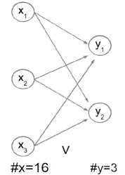
(a)

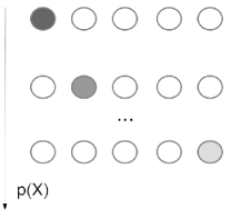
(b)

Figure 1: (a) Basic scheme of the network considered here. An array of inputs $x$ is connected via feed-forward connections $V$ to neurons generating outputs $y$. (b) Simple depiction of the inputs applied in the simulations in Figures 2 and 3. Every input pattern contains only one (out of 16) active input channel. The probability of a given $x$ to be applied to the network linearly grows with the index number of this active channel (see text).

The weights of synaptic connections from input $j$ (with activity $x_{j}$) to neuron $i$ (with activity $y_{i}$) are given by the matrix entry $V_{ij}$. The network’s architecture is schematically shown in Figure 1.

To obtain a set of learning rules, leading the network to optimization of a desired function $F$ through learning, one can consider learning as gradient descent optimization of $F$. Therefore, we put $\partial_{t}V_{ij}=\lambda\partial_{w_{ij}}F$ with some constant $\lambda$. For simplicity, we assume $\lambda=1$ and do not explicitely write it further. To quantitatively measure information inference from the input $x$, we use mutual information:

$$M(x,y)=\sum_{x}p(x)\sum_{y}p(y|x)\ln p(y|x)-\sum_{y}p(y)\ln p(y)$$ (4)

between inputs $x$ and outputs $y$. In order to balance information inference and energy consumption, we now need to add an energy consumption term $E$ to be subtracted from the information measure yielding:

$$F=M-\gamma E$$ (5)

to be optimized, with $\gamma$ a parameter. In this case:

$$\partial_{t}V_{ij}=\partial_{V_{ij}}F$$ (6)

provides a learning rule balancing information representation and energy consumption.

3 Results

3.1 Learning rules derivation

We first consider optimization of information inference with $F=M$. Every neuron receives signals from input channels independent from neuronal activity itself. This fact allows the decomposition $p(y|x)=\prod p_{i|x}$ with $p_{i}$ standing for the probability that the output neuron $i$ spikes ($y_{i}=1$), or doesn’t spike ($y_{i}=0$). $p(y_{i}=1|x)=f(I_{i})$ with $I_{i}=\sum_{j}V_{ij}x_{j}$ as the total input to the neuron $i$. Conversely, $p(y_{i}=0|x)=1-p(y_{i}=1|x)$. One can then write $p_{i}=y_{i}f(I_{i})+(1-y_{i})(1-f(I_{i}))$. Using that, we get the expression for $\partial_{V_{ij}}M$:

$$\partial_{V_{ij}}M=\sum_{x}\sum_{y}p(x)p(y|x)/p_{i|x}x_{j}(2y_{i}-1)f^{/}(I_{i})\,(\ln p(y|x)-\ln p(y)),$$ (7)

which with $p(x)p(y|x)=p(x,y)$ results in the rule for $V$ updates:

$$\Delta V_{ij}=x_{j}(2y_{i}-1)f^{/}(I_{i})/\{y_{i}f(I_{i})+(1-y_{i})(1-f(I_{i})\}\,(\ln p(y|x)-\ln p(y))$$ (8)

with $\ln p(y|x)=\sum_{i}\ln p_{i|x}=\sum_{i}\ln\{y_{i}f(I_{i})+(1-y_{i})(1-f(I_{i}))\}$ for every time an input is presented. $p(y_{i})$ can be expressed via the averaged activity $\bar{y}_{i}=<y_{i}p(y_{i})>=p(y_{i}=1)$, and for a system of only one output neuron, or in the approximation of uncorrelated output neurons, $\ln p(y)=\sum_{i}\ln(y_{i}\bar{y_{i}}+(1-y_{i})(1-\bar{y_{i}}))$. For these cases, the learning rule can be formulated explicitly after summing over $y_{i}\in\{0,1\}$ as:

$$\partial_{t}V_{ij} =\partial_{V_{ij}}M=\sum_{x}p(x)xf^{/}(I)\bigg{\{}\ln\frac{p(y=1|x)}{p(y=0|x)}-\ln\frac{p(y=1)}{p(y=0)}\bigg{\}}$$

$$=\bigg{\langle}xf^{/}(I)\bigg{\{}\ln\frac{f(I)}{1-f(I)}-\ln\frac{\bar{y}}{1-\bar{y}}\bigg{\}}\bigg{\rangle}=<xf^{/}(I)(g(f(I))-g(\bar{y})>$$ (9)

with $g(\epsilon)=\ln\frac{\epsilon}{1-\epsilon}$. This rule is remarkably similar to the Bienenstock-Cooper-Munro (BCM) learning rule (it differs in the particular form of the function $g$) [16].

Usually, however, the outputs caused by shared inputs are not independent from each other, and for a large output layer, a direct estimation of $p(y)$ is not obvious. One of a number of natural suggestions, which we used in simulations, is to approximate $p(y)$ using probabilities of states of single neurons, and of pairs of single neurons, which can be obtained by measuring the output covariance $<y_{i}y_{j}>$ of neuron pairs. Assuming vanishing non-trivial third and further cumulants, $p(y)$ can be written as a sum of products of $p(y_{i},y_{j})$. One of the possible simple implementable approximations is $\ln p(y)\sim\sum_{i}\ln p(y_{i})+\ln\frac{1}{N(N-1)}\sum_{i,j\neq i}\frac{p(y_{i},y_{j})}{p(y_{i})p(y_{j})}$.

3.2 Energy supply

The computational power of a neural network is bound by the amount of available resources, such as a restricted energy supply. To take into account a desirable minimization of the energetic costs of computation, we introduce the energy term:

$$E=\bigg{\langle}\sum_{i}(c_{sp}y_{i}+c_{psp}\sum_{j}V_{ij}x_{j})\bigg{\rangle}=\sum_{x}p(x)\bigg{(}\sum_{y}\{(\sum_{i}y_{i})p(y|x)\}+c_{psp}\sum_{j}V_{ij}x_{j}\bigg{)}$$ (10)

and optimize $\alpha M-\beta E$, or, for shortness, $F=M-\gamma E$ with $\gamma=\frac{\beta}{\alpha}$, with $\alpha$ and $\beta$ reflecting the relative importance of information inference and energy consumption. The first term in the expression for $E$ describes the energetic costs of output spikes (with constant $c_{sp}$), and the second the energetic costs of postsynaptic potentials (with constant $c_{psp}$). $\partial_{t}V_{ij}=\partial_{V_{ij}}F=\partial_{V_{ij}}M-\gamma\partial_{V_{ij}}E$ gives the new learning rule optimizing $F$. $\partial_{V_{ij}}M$ was obtained in the previous subsection, and thus:

$$\partial_{V_{ij}}E =\sum_{x}p(x)\bigg{\{}c_{sp}\sum_{y}\{\partial_{V_{ij}}p(y|x)(\sum_{k}y_{k})\}+c_{psp}x_{j}\bigg{\}}$$

$$=\sum_{x}p(x)\bigg{\{}c_{sp}\sum_{y}\bigg{\{}p(y|x)\frac{\partial_{V_{ij}}p(y_{i}|x)}{p(y_{i}|x)}(\sum_{k}y_{k})\bigg{\}}+c_{psp}x_{j}\bigg{\}}$$

$$=\sum_{x}p(x)\{c_{sp}x_{j}f^{/}(I_{i})+c_{psp}x_{j}\}$$

$$=\sum_{x}p(x)x_{j}\bigg{\{}c_{sp}p(y_{i}=1|x)\frac{f_{i}^{/}(I_{i})}{f(I_{i})}+c_{psp}\bigg{\}},$$ (11)

where we grouped possible values of $y$ in pairs differing only in values of $y_{i}$. The resulting learning rule is given by:

$$\partial_{t}V_{ij}=\sum_{x}\sum_{y}p(x)\bigg{\{}\frac{p(y|x)}{p_{i|x}}x_{j}(2y_{i}-1)f^{/}(I_{i})\,(\ln p(y|x)-\ln p(y)-\gamma c_{sp})-\gamma c_{psp}\bigg{\}},$$ (12)

and implementing weight updates every time an input is presented:

$$\Delta V_{ij}=x_{j}f^{/}(I_{i})(2y_{i}-1)/p_{i|x}\bigg{\{}(\ln p(y|x)-\ln p(y))-\gamma c_{sp}(\sum_{i}y_{i})\bigg{\}}-\gamma c_{psp}x_{j}.$$ (13)

Alternatively, we get $\Delta V_{ij}=x_{j}f^{/}(I_{i})\,\{(2y_{i}-1)(\ln p(y|x)-\ln p(y))/p_{i|x}-\gamma c_{sp}\}-\gamma c_{psp}x_{j}$ or $\Delta V_{ij}=x_{j}f^{/}(I_{i})(2y_{i}-1)/p_{i|x}\,\{(\ln p(y|x)-\ln p(y))\}-\gamma c_{sp}y_{i}\}-\gamma c_{psp}x_{j}$. Different implementations of the rule for weight updates are possible because of the relation between $f(I_{i})$ and $p(y_{i}=1)$. However, for slow enough learning, all of them produce the same weights dynamics, and since the last two forms do not require additional summation over all neurons to obtain the total current activity of the network, they make for a simpler implementation. The first form yields simpler understanding of the weights’ evolution tendencies and was used in simulations.

The terms proportional to $\gamma$ contribute to a reduction in precision of information inference to limit energy consumption. This is illustated in simulations for a simple network with $N=3$ output neurons and $K=16$ input neurons (Figure 2). Every presented input contains only one active input channel, with the probability of appearence of the input with the $k$’th active channel being proportional to $k\in[1,...,K]$ $p(x_{k})=(k_{0}+k)/s_{k}$ with normalization factor $s_{k}=\frac{K(K+1+2k_{0})}{2}$. For simulations, $f(u)=1/(1+\exp(-b(u-u_{0})))$ with $u_{0}=0.5$ and $b=10$, and $k_{0}=15$.

Adding energetic considerations to the derivation of the learning rule has the effect of rearrenging the correspondence between inputs and outputs. For highly probable outputs, $-\ln p(y)$ has low values. So, at equilibrium, more energetically expensive states with a high number of active neurons are more rare. On the other side, at the onset of learning, the term $\{(\ln p(y|x)-\ln p(y)-\gamma(\sum_{i}y_{i})\}$ is more often positive for energetically cheap network responses. As a consequence, input patterns occuring with high probabilities will evoke energetically cheap responses, involving a low number of neurons into coding. Rare events, on the contrary, can recruit a higher number of neurons for coding. Simulation results illustrating this rearrengement are presented in Figure 3, showing the relation between $|y|_{1}=\sum_{i}y_{i}$ and $p(x)$, as well as with $\gamma$. One way to interpret these results is to see every input $x$ as searching during learning for some output state $y$ to occupy, with $y$ states already occupied by a different input being more difficult to occupy. This effect is compounded by energetic terms. Additionally, rare events only lead to small modifications in the formation of connections shared with inputs presented more often. In the next subsection, we consider unreliable synapses and demonstrate that in this case too, rare inputs are effectively cut off by learning.

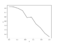
(a)

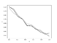
(b)

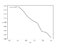
(c)

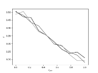
(d)

Figure 2: (a) Mutual information between the network’s inputs and outputs decreases as energetic constraints are applied ($\gamma>0$). (b) Similarly, the activity of the $N=3$ output neurons decreases as energetic constraints are applied. In both (a) and (b), $c_{sp}=1$ and $c_{psp}=0$. (c) Same as in (a) but plotted versus the energetic cost associated with post-synaptic potentials ($c_{psp}$). (d) Same as in (b) but plotted versus the energetic cost associated with post-synaptic potentials. In both (c) and (d), $\gamma=1$ and $c_{sp}=0$.

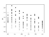
(a)

(b)

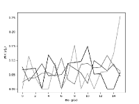
(c)

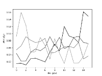
(d)

Figure 3: Energetic constraints map frequent inputs to low energy orbits. (a) Averaged network activity $|y|_{1}$ in response to inputs with increasing probabilities $p_{x}$ plotted versus the energetic cost of spikes (with $c_{sp}=1$ and $c_{psp}=0$). The probability of inputs is coded in shades of gray, from least (black) to most probable (increasingly lighter shades of gray). When energetic constraints are absent ($\gamma=0$), inputs presented more frequently evoke larger responses in the network and there is a distinct correlation between frequency of presentation and intensity of evoked responses (dots roughly organised from most probable, light gray, on top, to least probable, black, at the bottom). This relation starts to invert as $\gamma>0$ and is completely reverted at $\gamma=1$, with the most probable inputs (light gray) now being mapped onto orbits with very low averaged network activity, and the least probable inputs (black) now being mapped onto orbits with higher activity. (b) Averaged network activity $|y|_{1}$ evoked by inputs in different channels for $\gamma=0$ (black) and increasing values of $\gamma>0$ (increasinlgy lighter shades of grey). At $\gamma=0$, evoked activity is more or less even whether inputs are presented with low or high probability. As $\gamma$ increases, inputs presented with high probability (channels with high indices) evoke low activity while inputs presented with low probability (channels with low indices) evoke high activity. The overall activity decreases as $\gamma$ increases (from dark to light shades of grey). (c) and (d) illustrate the mapping of inputs induced by energetic contraints. (c) Probability of presentation of a specific input channel given the observed summed output activity $|y|_{1}=0$ (black) or $|y|_{1}=1,2,3$ (increasingly lighter shades of grey). In the absence of energetic constraints ($\gamma c_{sp}=0$), all input channels are more or less equiprobable. (d) Same as in (c) but with energetic constraints ($\gamma c_{sp}=0.3$). Now the most probable inputs (#14 and #15) most likely evoke no activity (black line), while rare inputs (#0, #1 and #2) most likely evoke maximal activity (all $N=3$ output neurons activated; lightest line).

3.3 Inference with unreliable input channels

Input signals reaching the brain from primary sensory neurons can also be unreliable. This fact can be modelled by adding Gaussian noise with variance $\sigma_{nz}$ to the input channels. In this scenario, large synaptic weights will amplify the noise and should be avoided. Derivation of learning rules taking input noise into account leads to an additional term proportional to $-\sigma_{nz}^{2}V$, which effectively implements a form of regularization. Similar considerations are also presented in reference [34]. The derivation is given in the Appendix.

This regularization term prevents the network from learning rare input events, whose low appearance frequency does not allow distinguishing them from random inputs induced by the noise in input channels. As a result, the evoked network responses grow in intensity as the probability of input patterns decay, until said probability decays down to the noise level. For input probabilities beyond that, and below the noise level, the network’s activity vanishes. As a consequence, the network’s response is strongest for moderately probable input patterns, rare, but still distinguishable from the noise. This is illustrated in Figure 4.

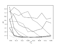
(a)

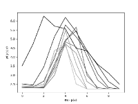
(b)

Figure 4: Learning in the presence of noise. (a) Averaged activity $|y|_{1}$ of the network’s response with $\gamma=1$, $c_{psp}=0.1$, $c_{sp}=0.3$ and input noise $\sigma_{nz}^{2}$ changing in arithmetic progression from $0.04$ to $0.4$ for different input patterns from low probability of occurence (black line) to higher probabilities of occurence (increasingly lighter shades of grey). As the noise level increases, inputs with low probability of occurence (darker shades) exhibit decaying activities and, eventually, aren’t learned by the network. (b) Probability of presentation of a specific input channel given the observed summed output activity $|y|_{1}$ is plotted for increasing noise intensities $\sigma_{nz}^{2}$ (dark to light shades of grey). As in Figure 2b, activity decays with the probability of presentation (increasing channel index). Additionally, the presence of noise ($\sigma_{nz}^{2}>0$) leads to a reduction of activity for channels corresponding to very rare inputs that cannot be distinguished from the noise. As a result, the peak of activity occurs for the same moderately probable $p_{x}$. The width of the distribution decreases with increasing noise intensities.

4 Conclusions and Discussion

The human brain consumes vasts amounts of energy with respect to its mass in the body (see [12] for a recent review). It is thus natural to assume that energetic constraints play an important role in shaping activity patterns and learning in neural networks, and a large body of experimental literature supports this assumption. Here, we addressed this question in a simple neural network model consisting of stochastic non-linear Hawkes neurons. Specifically, we started by deriving for this neural network a simple learning rule maximising information inference between inputs and outputs. For this, we used mutual information as the measure of information inference quality.

That learning rule includes terms of temporally and spatially local covariances, and a non-local value common to all neurons. A similar structure for learning rules, also derived by gradient descent on a goal function, is reported in [17], where the learning rule is derived as optimization of the squarred error for the network performing independent component analysis, and in [4], optimizing Kullback-Leibler divergence by teaching the network to reproduce a given set of input patterns developing in time. The non-local term is a function of the whole network activity and can be interpreted, e.g., as a slow non-local signal distributed throughout the network such as a neuromodulator [33, 45, 42, 18], GABA [32], $NO$ [41], or maybe a glial signal [14]. The local covariance-sensitive parts of the learning rule could be realized via spike-time dependent plasticity mechanisms. The difference between those terms – local temporal and spatial covariances on one hand, and the non-local value averaged over time on the other hand – implies a plasticity mechanism comparing the properties of ongoing activity to its recent past, similar to the BCM learning rule, which is also known to be related to optimization of information measures [16]. Qualitatively, terms in $M$ including $p(y|x)$ characterize the specificity of the network’s responses to various inputs, while terms including $p(y)$ characterize the efficient use by the network of the output space. This was implemented here with the covariance of single pairs of neurons, each of which can be measured locally. Another possible implementation could be the existence of intermediate inhibitory neurons in the network in a manner described in [24], but this will require further studies.

Taking energy consumption minimization into account results in new effects due to the additional terms in the learning rule. First, mutual information reaches lower saturation values, representing the trade-off between the quality of information inference and smaller synaptic weights, which limit energy consumption. Also, the probability of energetically expensive network responses decreases, and these become less probable than energetically cheaper responses. Regularly occuring inputs tend to evoke energetically cheap responses involving fewer neurons. Finally, taking input noise into account modifies learning so that very rare inputs are ignored, if they are so rare that they can’t be distinguished from the noise. If the number of neurons in the network is large enough to allow for a unique representation of every input, i.e. $p(y|x)$ is approximately 1 or 0, then from Equation (13), it follows that $p(y)\sim\exp(-\gamma c_{sp}|y|)$ with $|y|=\sum_{i}y_{i}$ for $c_{psp}=0$, with $c_{psp}>0$ only reducing $p(y)$. A similar exponential dependency is obtained in [40] when the network optimizes information representation under energy constraints for the probability of a random neuron to exhibit a given rate value. Both results can be seen as a Huffman-like [15] economical coding scheme, whereby energy savings are also taken into account.

In further studies, we plan to apply the method demonstrated here to time-dependent inputs, networks of excitatory and inhibitory neurons, and population coding. Similar to the ideas applied in [4] and [26] for likelihood measures, we propose to apply the approach presented here to time-dependent inputs considering every time sequence of a given time length as a single input, and optimizing a goal function for a set of these inputs. We have not yet taken into account Dale’s principle, the experimentally observed separation of neurons into distinct excitatory and inhibitory populations with exclusively positive, or negative, outgoing weights. Preliminary results for time-dependent inputs suggest a rough connection between inhibition and energy savings. Although generation of inhibition also requires energy (but see [7]), inhibitory effects help to avoid non-necessary spiking. In agreement with this thought, oscillations can also be considered as a self-organized way of saving energy by population coding, as recently demonstrated in [6]. More generally, one can study the relation between excitation, inhibition, the competition between information inference and energy savings, and self-organized criticality in neural networks inspired by arguments recently reviewed in [46].

Appendix

If neurons receive noisy inputs $x+\xi$ with $<\xi>=0,\ <\xi^{2}>=\sigma_{nz}^{2}$ when an input $x$ is presented, then the probability to fire in response to input $x$ is $p(y=1|x)=\int f(V(x+\xi))d\xi=G(Vx,|V\sigma_{nz}|^{2})$ with $G(I,\sigma_{I}^{2})$ defined as $G=\frac{1}{\sqrt{2\pi}\sigma_{I}}\int f(I+\xi)\exp(-\frac{\xi^{2}}{2\sigma_{I}^{2}})d\xi$. Both $I$ and $\sigma_{I_{i}}^{2}=\sum_{i}V_{ij}^{2}\sigma_{nz}^{2}$ depend on $V_{ij}$, and:

$$\partial_{V_{ij}}M =\sum p_{x}\{x_{j}\partial_{I}G+\partial_{V_{ij}}\sigma_{I}\partial_{\sigma}G\}\bigg{\{}\ln\frac{G(Vx,|V\sigma_{nz}|^{2})}{1-G(Vx,|V\sigma_{nz}|^{2})}-\ln\frac{p(y_{i}=1)}{1-p(y_{i}=1)}\bigg{\}}$$

$$=\sum p_{x}\{x_{j}\partial_{I}G+\frac{V_{ij}\sigma_{j}^{2}}{\sigma_{I}}\partial_{\sigma_{I}}G\}\bigg{\{}\ln\frac{G(Vx,|V\sigma_{nz}|^{2})}{1-G(Vx,|V\sigma_{nz}|^{2})}-\ln\frac{p(y_{i}=1)}{1-p(y_{i}=1)}\bigg{\}}$$ (14)

now contains an additional term proportional to $\frac{V_{ij}\sigma_{j}^{2}}{\sigma_{I}}$ when compared to the noiseless case. This term is usually negative, meaning that larger synaptic weights increase uncertainty. It also does not vanish for $x_{j}=0$, effectively acting as a leak term for the synaptic weight dynamics.

For the particular choice of $f(I)=H(I-\theta)$ as a step function, one gets $G(I,\sigma)=1-\Phi(\frac{\theta-I}{\sigma})=0.5-0.5erf(\frac{\theta-I}{\sqrt{2}\sigma})$ and $\partial_{\sigma}G=\frac{\theta-I}{\sqrt{2\pi}\sigma^{2}}\exp(\frac{-(\theta-I)^{2}}{2\sigma^{2}})=\frac{\theta-I}{\sigma}\partial_{I}G$. (Additionally, some stochasticity in the neuronal output can be modelled by adding the constant $\sigma_{y}^{2}$ to $\sigma_{I}^{2}$.)

To obtain a learning rule operating with $\tilde{x}=x+\xi$ instead of $x$, if the network only receives noisy itput, one can rewrite $\partial_{V}M$ as:

$$\partial_{V}M =\sum p(\tilde{x})\tilde{x}f^{/}(V\tilde{x})\bigg{\{}\int p(\xi)\ln\frac{G(\tilde{x}-\xi,\sigma)}{1-G(\tilde{x}-\xi,\sigma)}d\xi-\ln\frac{p(y=1)}{p(y=0)}\bigg{\}}$$

$$+\sum p(\tilde{x})p(y|\tilde{x})\bigg{\{}\int p(\xi)\bigg{[}(\tilde{x_{j}}-\xi_{j})\partial_{I}+\frac{V_{ij}\sigma_{j}^{2}}{\sigma_{I}}\partial_{\sigma_{I}}\bigg{]}\ln p(y|(V(\tilde{x}-\xi),\sigma_{I}^{2}))d\xi\bigg{\}}$$ (15)

with $p(y|\tilde{x})=[1-y+f(V\tilde{x})(2y-1)]$. For a particular form of $f$ and $G$, integration over $\xi$ can be performed to get a new learning rule. For the above-mentioned step function, one can exploit the relation $\partial_{\sigma}G=\frac{\theta-I}{\sigma}\partial_{I}G$. Considering input from channel $j$ and from all other channels in neuron $i$ separately, one obtains by integration in the leading order of $\sigma_{nz}$ an approximation for $\partial_{V_{j}}M\sim p(\tilde{x})\{p^{/}(y|\tilde{x})\tilde{x}-V_{j}\sigma_{j}^{2}/\sigma_{I}^{2}p(y|\tilde{x})\}\ln\frac{p(y|\tilde{x})}{p(y)}$ with a new noise-induced term proportional to $-V_{j}\sigma_{j}^{2}/\sigma_{I}^{2}$.

References

- [1] A. Bell, T. Sejnowski (1995) An information-maximization approach to blind separation and blind deconvolution. Neural Comput. 7 (6): 1129–59
- [2] R. Bourdoukan, D. Barrett, S. Deneve, C. Machens (2012) Learning optimal spike-based representations. Advances in Neural Information Processing Systems 25:2285-2293
- [3] M. Boerlin, C. Machens, S. Deneve (2013) Predictive coding of dynamical variables in balanced spiking networks. PLoS Computational Biology 9(11):e1003258
- [4] J. Brea, W. Senn, J.-P. Pfister. (2011) Sequence learning with hidden units in spiking neural networks. NIPS 2011:1422-1430.
- [5] N. Brunel, J.-P. Nadal. Mutual information, Fisher information and population coding. Neural Computation, Massachusetts Institute of Technology Press (MIT Press), 1998, 10 (7), pp.1731 - 1757.
- [6] M. Chalk, B. Gutkin, S. Deneve (2016) Neural oscillations as a signature of efficient coding in the presence of synaptic delays. eLife 5:e13824.
- [7] J.-Y. Chatton, L. Pellerin, P. J. Magistretti (2003) GABA uptake into astrocytes is not associated with significant metabolic cost: Implications for brain imaging of inhibitory transmission. Proc. Nat. Acad. Sci. USA 100(21): 12456-12461.
- [8] G. Chechik (2003) Spike-Timing Dependent Plasticity and Relevant Mutual Information Maximization. Neural Comput. 15(7):1481-1510.
- [9] M. Conrad, E. Engl, R. B. Jolivet (2018) Energy use constrains brain information processing. Tech. Digest - IEDM 11.3.1-11.3.3
- [10] E. Engl, R. B. Jolivet, C. N. Hall, D. Attwell (2017) Non-signalling energy use in the developing rat brain. J. Cereb. Blood Flow Metab. 37(3):951-966.
- [11] J. J. Harris, E. Engl, D. Attwell, R. B. Jolivet (2019) Energy-efficient information transfer at thalamocortical synapses. PLOS Comput. Biol.
- [12] J. Harris, R. Jolivet, D. Attwell (2012) Synaptic Energy Use and Supply. Neuron 75:(5)762-777.
- [13] J. J. Harris, R. B. Jolivet, E. Engl, D. Attwell (2015) Energy-Efficient Information Transfer by Visual Pathway Synapses. Curr. Biol. 25(24):3151-3160
- [14] C. Henneberger, T. Papouin, S. Oliet, D. Rusakov Long-term potentiation depends on release of D-serine from astrocytes. Nature 463, 232–236 (2010).
- [15] D. Huffman (1952) A Method for the Construction of Minimum-Redundancy Codes. Proceedings of the IRE. 40 (9): 1098–1101.
- [16] N. Intrator, L. Cooper (1992) Objective function formulation of the BCM theory of visual cortical plasticity: Statistical connections, stability conditions. Neural Networks 5:3-17.
- [17] T. Isomura, T. Toyoizumi. (2016) A Local Learning Rule for Independent Component Analysis. Scientific Reports, 6: 28073
- [18] J. Johansen et al. (2014) Hebbian and neuromodulatory mechanisms interact to trigger associative memory formation. Proc. Natl. Acad. Sci. USA 111, E5584–E5592
- [19] R. B. Jolivet, A. Rauch, H.-R. Lüscher, W. Gerstner (2005) Integrate-and-Fire models with adaptation are good enough: Predicting spike times under random current injection. Adv. Neural Inf. Process. Sys. 18:595-602
- [20] R. Jolivet, A. Rauch, H.-R. Lüscher, W. Gerstner (2006) Predicting spike timing of neocortical pyramidal neurons by simple threshold models. J. Comput. Neurosci. 21(1):35-49
- [21] R. B. Jolivet, P. J. Magistretti, B. Weber (2009) Deciphering neuron-glia compartmentalization in cortical energy metabolism. Front. Neuroenerg. 1 4
- [22] L. Kostal, R. Kobayashi (2015) Optimal decoding and information transmission in Hodgkin-Huxley neurons under metabolic cost constraints. BioSystems 136:3-10
- [23] L. Kostal, S. Shinomoto (2016) Efficient information transfer by poisson neurons. Math. Biosci. Engineer. 13(3):509-520
- [24] B. Nessler, M. Pfeiffer, L. Buesing, and W. Maass. Bayesian computation emerges in generic cortical microcircuits through spike-timing-dependent plasticity. PLOS Computational Biology, 9(4):e1003037, 2013
- [25] J.-P. Nadal, N. Parga (1994) Nonlinear neurons in the low-noise limit: a factorial code maximizes information transfer. Network: Computation in Neural Systems 5(4):565-581
- [26] D. Kappel, B. Nessler, and W. Maass. STDP installs in winner-take-all circuits an online approximation to hidden Markov model learning. PLOS Computational Biology, 10(3):e1003511, 2014
- [27] W. Levy, T. Berger, M. Sungkar (2016) Neural Computation From First Principles: Using the Maximum Entropy Method to Obtain an Optimal Bits-Per-Joule Neuron. IEEE Transactions on Molecular, Biological and Multi-Scale Communications 2(2): 154 - 165
- [28] W. B Levy, R. Baxter. (2002) Energy-Efficient Neuronal Computation via Quantal Synaptic Failures. The Journal of Neuroscience, 22(11):4746–4755
- [29] R. Linsker (1988) Self-organization in a perceptual network. IEEE Computer. 21 (3): 105–17.
- [30] R. Linsker (1992) Local Synaptic Learning Rules Suffice to Maximize Mutual Information in a Linear Network. Neural Computation 4 (5): 691-702
- [31] R. Linsker (1997) A local learning rule that enables information maximization for arbitrary input distributions. Neural Computation. 9 (8): 1661–65.
- [32] V. Paille et al. (2013) GABAergic Circuits Control Spike-Timing-Dependent Plasticity. J. Neurosci. 33, 9353–9363
- [33] J. Reynolds, B. Hyland, J. Wickens. (2001) A cellular mechanism of reward-related learning. Nature 413, 67–70
- [34] D. Rezende, D. Wierstra, W. Gerstner. (2011) Variational learning for recurrent spiking networks. NIPS’11 Proceedings: 136-144
- [35] B. Sengupta, S. Laughlin, J. Niven (2013) Balanced Excitatory and Inhibitory Synaptic Currents Promote Efficient Coding and Metabolic Efficiency. PLoS Comput Biol 9(10): e1003263
- [36] B. Sengupta, M. Stemmler, K. Friston. (2013) Information and efficiency in the nervous system - a synthesis. PLoS Comput Biol. 9(7):e1003157
- [37] M. Stemmler, C. Koch (1999) How voltage-dependent conductances can adapt to maximize the information encoded by neuronal firing rate. Nat Neurosci. 2(6):521-7.
- [38] G. Tkacik, J. Prentice, V. Balasubramanian, E. Schneidman (2010) Optimal population coding by noisy spiking neurons. Proc Natl Acad Sci U S A. 107(32):14419-24
- [39] T. Toyoizumi, J.-P. Pfister, K. Aihara, W. Gerstner. (2004) Spike-Timing Dependent Plasticity and Mutual Information Maximization for a Spiking Neuron Model. Advances in Neural Information Processing Systems 17 (NIPS 2004)
- [40] Y. Tsubo, Y. Isomura, T. Fukai (2012) Power-Law Inter-Spike Interval Distributions Infer a Conditional Maximization of Entropy in Cortical Neurons. PLoS Comput Biol 8(4): e1002461
- [41] S. Vincent (2010) Nitric oxide neurons and neurotransmission, Progress in Neurobiology 90(2):246-255.
- [42] S. Yagishita et al. (2014) A critical time window for dopamine actions on the structural plasticity of dendritic spines. Science 345, 1616–1620
- [43] L. Yu, Y. Yu (2017) Energy-efficient neural information processing in individual neurons and neuronal networks. J Neurosci Res. 95(11):2253-2266
- [44] L. Yu, Ch. Zhang, L. Liu, Y. Yu (2016) Energy-efficient population coding constrains network size of a neuronal array system. Scientific Reports 6:19369
- [45] J. Zhang, P. Lau, G. Bi. (2009) Gain in sensitivity and loss in temporal contrast of STDP by dopaminergic modulation at hippocampal synapses. Proc. Natl. Acad. Sci. USA 106: 13028–13033
- [46] Sh. Zhou, Y. Yu (2018) Synaptic E-I Balance Underlies Efficient Neural Coding. Front Neurosci. 12: 46