Lightweight Composite Re-Ranking for Efficient Keyword Search with BERT

Abstract.

Recently transformer-based ranking models have been shown to deliver high relevance for document search and the relevance-efficiency tradeoff becomes important for fast query response times. This paper presents BECR (BERT-based Composite Re-Ranking), a lightweight composite re-ranking scheme that combines deep contextual token interactions and traditional lexical term-matching features. BECR conducts query decomposition and composes a query representation using pre-computable token embeddings based on uni-grams and skip-n-grams, to seek a tradeoff of inference efficiency and relevance. Thus it does not perform expensive transformer computations during online inference, and does not require the use of GPU. This paper describes an evaluation of relevance and efficiency of BECR with several TREC datasets.

1. Introduction

The advent of transformer architectures (e.g., BERT) and pretraining techniques rejuvenated neural ranking studies using deep contextual models (e.g.  (MacAvaney et al., 2019; Dai and Callan, 2019; Lin et al., 2020)), leading to a higher relevance score in text document search. However, the cost of runtime transformer-based inference is still very expensive. To address this limitation, recent studies examined the efficiency of transformer-based models during model inference (MacAvaney et al., 2020a; Dai and Callan, 2019; Hofstätter et al., 2020b; Khattab and Zaharia, 2020). Nonetheless, devising a fast online ranking scheme with a relevance comparable to those of expensive transformer-based schemes remains a critical problem, especially on a CPU-only server without GPU support. To reduce the complexity involved in the transformer computation, simplified BERT based (Devlin et al., 2019) architecture was previously proposed to reduce the burden of jointly encoding query-document pairs, including the dual encoder based rankers that separately computes the query and document representations (Khattab and Zaharia, 2020; Zhang et al., 2020a). With dual encoder models, the BERT representations of documents become independent of the queries and can thus be pre-computed. However, expensive transformer computation still needs to be conducted during online inference as queries are dynamic.

Considering that short keyword queries account for a majority of web search traffic (Bond, 2020), where the average number of words in user queries of popular search engines is between two and three (Jansen and Spink, 2006), our approach takes a further step on top of the previously proposed dual-encoder design (MacAvaney et al., 2020a; Khattab and Zaharia, 2020). We propose a lightweight neural re-ranking scheme named BECR that composes a query representation using pre-computable token embeddings based on uni-grams and skip-n-grams. This representation composition does not require expensive transformer-based inference for an input query during runtime, and thus GPU support is not necessary. In addition, BECR leverages the classical lexical matching features to offset the relevance degradation from the above approximation, and use hashing (Ji et al., 2019) and distilling (MacAvaney et al., 2020a) to reduce storage cost.

Our evaluation with several TREC datasets shows that this re-ranking scheme can deliver decent relevance performance compared to the other baselines. Because BECR’s online computation complexity is significantly smaller, the main contribution of this work is to provide a lightweight and CPU-friendly online neural inference scheme to strike an efficiency and relevance tradeoff. Since adding a high-end GPU incurs significant monetary cost and energy consumption, the design of BECR can be attractive for fast query processing on servers without GPU support.

2. Background and Related Work

The problem of top $K$ text document re-ranking is defined as follows: given a query $q$ and candidate documents, form text features for each document and rank documents based on these features. We focus on ad-hoc search where a query contains several keywords.

Large-scale search systems typically deploy a multi-stage ranking scheme. A common first-stage retrieval model uses a simple algorithm such as BM25 (Jones et al., 2000) to collect top documents. The second or later stages use a more advanced algorithm to further rank top documents. This paper focuses on re-ranking in the second stage for a limited number of top documents. Below we review the previous studies in this field and highlight the key difference of our method.

Deep contextual ranking models. Neural interaction based models such as DRMM (Guo et al., 2016) and (Conv-)KNRM (Dai et al., 2018; Xiong et al., 2017) have been proposed to leverage word embeddings for ad-hoc search. Compared to traditional ranking methods such as LambdaMART (Liu, 2010), these models provide a good NDCG (Järvelin and Kekäläinen, 2002) score on TREC datasets. However, their contextual capacity is limited by using non-contextual uni-gram embeddings. In recent years, the transformer based model BERT has been adopted (Devlin et al., 2019) to re-ranking tasks (Nogueira and Cho, 2019; Yang et al., 2019; Dai and Callan, 2019; Nogueira et al., 2019; Li et al., 2020; Hofstätter et al., 2021). The merger of BERT models with interaction based neural IR models has also been investigated (MacAvaney et al., 2019; Hofstätter et al., 2020b; Mitra et al., 2020). Among them, several models (MacAvaney et al., 2019; Li et al., 2020; Dai and Callan, 2019; Yang et al., 2019) have achieved impressive relevance on keyword based queries. Work exploring zero-shot learning or weak supervision also demonstrates competitive performance on such ad-hoc datasets (ClueWeb and TREC Disk 4&5) (Nogueira et al., 2020; Sun et al., 2021; Zhang et al., 2020b, c; Yilmaz et al., 2019).

Efficiency optimization for transformer-based rankers. Although the aforementioned transformer based ranking achieves remarkable relevance, such an architecture is extremely expensive for online search systems due to the strict latency requirement (Lin et al., 2020). To this end, the dual-encoder or poly-encoder design that separately encodes the query and documents has been studied (Zhan et al., 2020a; Chen et al., 2020; Khattab and Zaharia, 2020; Reimers and Gurevych, 2019; Karpukhin et al., 2020; Zhang et al., 2020a; Humeau et al., 2020; Zhan et al., 2020b; Lu et al., 2020). Among them, ColBERT (Khattab and Zaharia, 2020) applies a BERT based dual-encoder design on re-ranking and retrieval. MORES (Gao et al., 2020a) framework separating the representation and interaction phase of query and documents achieves 120x speed up in inference compared to a BERT ranker. TwinBERT (Lu et al., 2020) is a lightweight transformer based dual-encoder distilled from a BERT cross-encoder teacher model. DC-BERT (Zhang et al., 2020a) applies a dual-encoder BERT on document retrieval for open domain Q&A tasks. These rankers greatly shorten latency through offline pre-computation of document representations while performing transformer computation to generate query representation at runtime.

In this paper, we adopt a dual encoder framework while further simplifying the online inference by decomposing queries to leverage pre-computed uni-gram and skip-n-gram embeddings. A skip-n-gram (Guthrie et al., 2006) is a set of words that appear in a document within certain appearance proximity constraint. To offset the relevance loss due to the above approximation, BECR combines semantic matching with lexical text matching signals such as term-frequency based features from BM25, and word distance based proximity (Bai et al., 2008; Zhao and Huang, 2014). Thus it is also motivated by the work (Mitra et al., 2017; Shao et al., 2019; Gao et al., 2020b; Luan et al., 2020) that investigates non-transformer based neural ranking with traditional text features.

There are other lines of work that improves the efficiency of transformer architectures, including compact attention based transformer architectures (Hofstätter et al., 2020b; Mitra et al., 2020; MacAvaney et al., 2020a), early exiting (Xin et al., 2020), cascading (Hofstätter et al., 2021; Soldaini and Moschitti, 2020), quantization (Zafrir et al., 2019), and sparse transformers  (Jiang et al., 2020; Hofstätter et al., 2020a). As they focus on the transformer model architectures, our proposed techniques are orthogonal to these models. Our work has also leveraged embedding approximation based on locality-sensitive hashing (Ji et al., 2019) to improve efficiency. Other related studies on efficiency and relevance trade-offs for transformer-based ranking includes models that learns the importance or likelihood of tokens in query and documents (Dai and Callan, 2020; Zhuang and Zuccon, 2021; MacAvaney et al., 2020b).

In the design of BECR’s ranking formula, we are inspired by a recent learning-to-rank study (Zhuang et al., 2020) that advocates additive models for better ranking interpretability. This additive nature simplifies the incorporation of other application-specific ranking features.

3. The Proposed Framework

This section presents our design considerations and the BECR re-ranking framework. Figure 1 illustrates the ranking structure of BECR with tri-encoding of documents, queries, and tokens. BECR separately encodes a query and a document, then considers the term-level interaction to capture semantic relatedness of a document with a query, and combines that with other types of relevance signals.

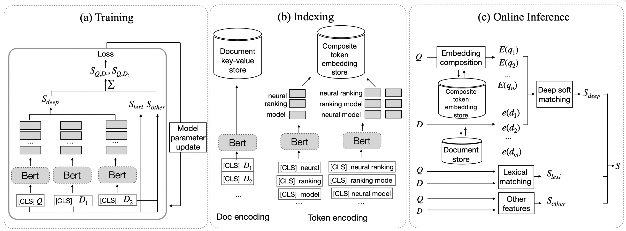
Figure 1. Training, Offline Processing and Online Inference in BECR

3.1. Embedding Composition for Queries

As discussed, previous dual-encoder rankers decouple the query and document encoding, and encode a query using BERT during online inference. During the training time, a BERT query encoding model is trained. During the indexing time, a query encoding model is stored with learned parameters. During the inference time, a ranker feeds a query through the pre-stored BERT query encoding model to produce a set of contextual embeddings for query terms.

To improve the online efficiency, we propose to approximate the deep representation of a query through a composition of pre-computed token embeddings based on uni-grams and skip-n-grams. Given a query composed of a set of terms $Q=\{q_{1},q_{2},\cdots,q_{n}\}$, and a document $D$ with $m$ terms, $d_{1},d_{2},...,d_{m}$, we decompose a query into a set of semantic token groups and denote it as $T$. In our evaluation, $T$ is a set of uni-gram tokens and token pairs within a context window size such as $|window|=3$ to control the number of pairs, meaning we only consider the token pairs within distance 3 inside the query.

The contextual embedding of each query term $q_{i}$ in a given query is defined as

(1) $$E(q_{i})=\sum_{t\in T\land contain(t,q_{i})}\frac{w_{t}}{\|w\|_{1}}e(q_{i}^{t})$$

where $e(q_{i}^{t})$ represents the pre-computed embedding vector of term $q_{i}$ in token group $t$, and $w_{t}$ is the weight factor for $t$. Predicate $contain(t,q_{i})$ means that token group $t$ semantically relates to term $q_{i}$.

In our evaluation described in Section 4 where a query term is a word token, and $t$ is either a word based token or a pair of such tokens, we simply define $contain(t,q_{i})$ to be true when $t$ contains $q_{i}$. $\|w\|_{1}$ is the 1-norm of all weights $w_{t}$ used so that they are normalized as a weight distribution. A uni-gram is weighted smaller than a token pair, while we impose a scaling factor for each token pair based on the word distance in a query. Specifically the weight of token pair $(a,b)$ is $\frac{1}{span(a,b)}$ where $span(a,b)$ is the word distance of words $a$ and $b$. The weight for the uni-gram will be defined as $\frac{1}{|window|+1}$.

For example, given query “neural ranking model”, the token group set $T$ for this query is $\{$neural, ranking, model, neural-ranking, neural-model, ranking-model$\}$. Assume all these token pairs and uni-grams have the embeddings available from the index. The embedding vector of term “neural” in this query will be:

$$(w_{1}\cdot e(\mbox{neural}^{\mbox{neural}})+w_{2}\cdot e(\mbox{neural}^{\mbox{neural-model}})$$

$$+w_{3}\cdot e(\mbox{neural}^{\mbox{neural-ranking}}))\frac{1}{\|w\|_{1}}$$

where $w_{1}$=0.25, $w_{2}$=0.5, $w_{3}$=1. Expression $e(\mbox{neural}^{\mbox{neural-model}})$ is the embedding of query term “neural” under token group “neural-model” computed during the offline indexing time.

Our current evaluation uses heuristically-determined weights for the above composition and we leave the weights exploration through machine learning to future work.

Figure 1 illustrates training, offline indexing, and online inference with query embedding composition in BECR using an example.

During the training time as depicted in Fig. 1(a), we input a set of training queries with their matched documents to the BECR model to learn model parameters in an end-to-end manner. Given training query $Q$ and matched documents $D_{1}$ and $D_{2}$, assuming $D_{1}$ is more relevant than $D_{2}$ for $Q$, the goal of training is to minimize a pairwise softmax loss. There are two methods to train the model. 1) We don’t decompose queries, and input the whole query and document separately into BECR using $[CLS]Q$ directly. 2) We decompose the query and compose the query embeddings based on Equation (1). In our evaluation, 1) is more effective for ClueWeb09-Cat-B and Robust04 with limited number of training queries. 2) is used for MS MARCO with more training queries.

During the indexing time as depicted in Fig. 1(b), we select a set of desired token groups (e.g. uni-gram tokens and token-pairs), and feed them to the trained model to pre-compute their embeddings. The results (after compression) are saved in a key-value store called composite token embedding store for online access.

During the inference time as depicted in Fig. 1(c), we decompose a query into a set of tokens, represent a query term embedding using token groups (e.g. uni-gram tokens, or token pairs), fetch the embedding of the token groups from the composite token embedding store. If some token pair embeddings are not found from the composite token embedding store, we can ignore them because we have at least the uni-gram embeddings to work with.

3.2. Online Composite Re-Ranking

We divide ranking signals into 3 components: deep contextual soft matching, lexical matching, and other features. To derive the final ranking score, we opt to use an additive combination of these components for simplicity. To get the component score, we use simple feed forward layer to combine the features. Note that others can easily add more components based on their applications or use a more complex architecture for composition.

To derive these weight parameters used in each component, the overall framework along with its component weights is trained end-to-end jointly. The final ranking score $S$ is the addition of a summary score from each component:

$$S=S_{deep}+S_{lexi}+S_{others}.$$

We use symbols $\alpha$, $\beta$ and $\gamma$ to represent the weight parameters in the three components, respectively.

The deep soft matching component. The deep semantic matching component adopts a deep learning architecture similar to the CEDR-KNRM model (MacAvaney et al., 2019; Xiong et al., 2017). Compared to CEDR-KNRM, we modify the final scoring such that it is decomposed into a set of subscores where each of them corresponds to a query term.

Note that a BERT-based embedding contains $L$ layers, and we denote the representation of query term $q_{i}$ under layer $l$ as $\boldsymbol{E}_{l,q_{i}}$. The similarity score $c_{l,i,j}$ between query term $q_{i}$ and document term $d_{j}$ under layer $l$ is computed as the cosine similarity between $\boldsymbol{E}_{l,q_{i}}$ and $\boldsymbol{E}_{l,d_{j}}$.

$$c_{l,i,j}= cosine(\boldsymbol{E}_{l,q_{i}},\boldsymbol{E}_{l,d_{j}}),$$

For each layer $l$, we group the similarity subscores for each query term using the $K$ RBF kernels following (Xiong et al., 2017), where $\mu_{k}$, $\sigma_{k}$ are the parameters of the k-th kernel. The subscore ($s_{l,i,k}$) for the query term $q_{i}$ under layer $l$ and kernel $k$ is defined as:

$$s_{l,i,k}= \log\sum_{1\leq j\leq m}(-\frac{(c_{l,i,j}-\mu_{k})^{2}}{2\sigma_{k}^{2}}).$$

where this document contains $m$ term. Note that in our model, $\mu_{k}$, $\sigma_{k}$ are trainable hyper-parameters hence there is no exact matching kernel as specified in KNRM model. We rely on the lexical component to capture exact matching information.

For each query term $q_{i}$, there are a total of $L*K$ features given $L$ BERT layers and $K$ kernels. The soft semantic matching score is the sum of all term subscores.

$$S_{deep}= \sum_{1\leq i\leq n}S_{deep,i}$$

$$S_{deep,i}= \sum_{1\leq k\leq K,1\leq l\leq L}\alpha_{k,i,l}s_{l,i,k}$$

where $\alpha_{k,i,l}$ is a weight parameter for subscore $s_{l,i,k}$.

The lexical matching component. We include a set of lexical matching features to complement the deep contextual soft matching component. In our evaluation, we use BM25 (Jones et al., 2000) for query words that appear in the title and body separately, and BM25 for query word pairs that appear in the title and body, plus other query word pair based proximity features (Bai et al., 2008; Zhao and Huang, 2014; Shao et al., 2019) with the minimum, maximum, and average of the squared min distance reciprocal of query word pairs in the title or in the body. The lexical score $S_{lexi}$ is obtained through a linear combination of all these signals.

Other features. We add the last layer’s [CLS] token representation of each document as document-specific features. There are other query independent or dependent features for each document used in traditional text ranking and web search applications. The examples of such signals include document quality, freshness and document-query click through rate. For the ClueWeb09-Cat-B dataset used in our evaluation, we have used a page rank score for each document. The other ranking component $S_{others}$ is the linear combination of all these features. The online inference can obtain these features from the inverted index or from a separate key-value store.

Section B in the appendix gives an example of ranking two documents for a query with BECR and illustrates the above scoring components and the trained weights.

3.3. Storage Cost and Reduction Strategies

As pointed out in (Lin et al., 2020), efficient neural ranking models need to take into account the storage cost in addition to query latency and effectiveness. The contextual nature of the transformer architecture implies that the same word in documents can have different contextual representations. Thus there is a significant storage requirement for hosting embedding vectors for a large number of documents.

Table 1. Sample online embedding storage cost for BECR

	Doc embeddings	Token embeddings
Original space	$4(mL$+$1)768D$	$4L(V$+$2H)768$
Compressed space	$(mL^{\prime}\frac{b}{8}+4*768)D$	$L^{\prime}(V+2H)\frac{b}{8}$
$m$=$857$,$V$=$14.5$M,$H$=$467$M	Orig: 1,711TB	Orig: 37.9TB
$L^{\prime}$=$5$, $b$=$256$, $D$=$50$M, $L$=$13$	Compress: 7.0TB	Compress: 152GB

Storage cost for document embeddings. Assuming the set of $D$ documents is not updated frequently, we encode each document using BERT with $L$ layers and save it in a key-value store. Table 1 gives an estimation of storage size in bytes for hosting embeddings of documents and semantic tokens in BECR with an example (before and after compression with an approximation). We assume the BERT-base model is used with the vector dimension of 768. To deal with long documents with more than 512 tokens, following (MacAvaney et al., 2019), we split the documents into even length texts and learn the token-level representation piece by piece. The [CLS] representation of the whole document is calculated by averaging the [CLS] representations of all text pieces from the document. Denoting the average length of a document as $m$ tokens for web documents, the storage space plus one extra [CLS] embedding vector is $4*(mL+1)*768$ bytes per document, as the values in a BERT term embedding vector is a 4-byte floating point. For a database with 50M documents and average length $m=857$, following the characteristic of ClueWeb09-Cat-B without spam document removal, the storage per document is 34.2MB and the total storage space is about 1,711TB. That is huge and unrealistic, even the size of this dataset can be further reduced by removing some spam documents as we did in Section 4.

The work of Ji et al. (Ji et al., 2019) proposes an embedding approximation based on locality-sensitive hashing (LSH). PreTTR (MacAvaney et al., 2020a) uses term representation compression, 16-bit floating point numbers, and distilling with a limited number of BERT layers to reduce the storage demand. ColBERT (Khattab and Zaharia, 2020) uses vector dimension reduction to decrease the embedding vector size from 768 to 128. BECR adopts some of these ideas. Our evaluation shows in Section 4 that decreasing the number of layer $L$ from 13 to 5 with a proper selection of layers does not lead to a noticeable impact on NDCG@5 relevance while there is a 0.01 point loss in NDCG@10 and NDCG@3. Thus choosing 5 layers can be a feasible strategy.

The major space reduction comes from LSH approximation. We reduce the size of each embedding vector from 768$\times$4 bytes to only $b$ bits while preserving the accuracy of cosine similarity between two approximated vectors. The estimation of cosine similarity between two embedding vectors uses the Hamming distance between their LSH footprints. In Table 6 of Section 4.3, we experiment with the tradeoff between NDCG scores and footprint dimension $b$. Our evaluation shows that the LSH footprint dimension with 256 bits (namely 32 bytes) can deliver a highly competitive relevance.

Last row of Table 1 lists the document embedding storage space after LSH hashing and setting $L^{\prime}=5$. The storage space need is reduced to about 138.7KB per document based on expression $857\times 5\times 256/8+4\times 768$ and the total is about 7.0TB for a 50 million document set with average length 857. Considering Samsung and Seagate have produced an internal 2.5” SSD drive with a large capacity varying from 8TB to 32TB for servers, and each server can host multiple internal drives, the above storage cost is reasonable for a production environment.

Storage cost for the composite token embedding store. This key-value store can be accessed by token group identifiers. In our evaluation, this store saves embeddings for uni-gram tokens and token pairs. Table 1 gives an estimation of storage size in bytes when the number of uni-grams tokens and token pairs is $V$ and $H$ respectively. Notice that each token pair has two vectors to represent its embedding while an uni-gram token has one vector. Without LSH approximation, the total number of bytes needed for token embedding storage would be $4L(V+2H)\times 768$ with a 32-bit floating point number.

We use the characteristics of the ClueWeb09-Cat-B dataset to show the cost of token embedding storage. This dataset has about V=14.5M uni-grams that appear more than once in documents, and H=467M word-pairs that appear more than once and within window size 2. The total cost is 37.9TB and thus aggressive compression with an approximation is desired. By using the 256-bit LSH footprint and 5 BERT layers for each token, the above storage is reduced to $32L^{\prime}(V+2H)$ bytes, which is about 152GB. If we include all uni-grams and word pairs within window 2, then $V=32.4$M and $H=940.3$M. The space cost is 305.5GB, which is still affordable.

Note that there are many ways to further adjust the choices of uni-grams and skip-n-grams based on an application dataset and its relevance study results for training instances. For example, one could add some restriction on the token set based on the BERT dictionary which uses WordPiece (Wu et al., 2016) tokenizer and the number of BERT uni-grams is around 32,000.

3.4. Discussion on Online Inference

Since a query term is represented by a set of token groups (e.g. tokens and token pairs) and the similarity angle of two LSH-based bit vectors is proportional to their Hamming distance scaled by the total number of bits. We approximate the cosine similarity between a query term and a document term in the LSH setting using the weighted linear combination of the cosine similarity between each of these token groups and a document term. These weights follow the ones used in Equation  1.

When processing each online query, we can break the inference into two steps. First, a serving system looks up the LSH footprint of the query token groups and the matched documents separately. Afterwards, it derives soft interaction between each selected token group and document terms through pair-wise hamming distance computation. Second, given the soft interaction scores of document term embeddings and query token embeddings based on their LSH footprints, we use the weighted linear combination to derive the similarity scores between query terms and document terms. Separately, the lexical features and other features would be passed down from the document retrieval stage of the search system. Then given the contextual score, lexical features, and other feature subscores, we compose the final ranking score.

We have implemented a key-value store to host document and composite token embeddings, and in our experiment with a Samsung 960 NVMe SSD, fetching one document embedding vector randomly costs 0.17 milliseconds (ms) with 5 layers, and 0.21ms with 13 layers, while fetching a token embedding takes about 0.058ms in a sequential I/O mode. Thus fetching 150 different document embeddings and about ten or less query token embeddings takes about 26ms in total for the 5-layer setting and 32ms for 13 layers. Such a cost is reasonable to accomplish interactive query performance.

The dominating part of online inference time complexity is the computation of query-document term interaction and kernel calculation with $L$ BERT layers, which is $\Theta(n\cdot m\cdot p+n\cdot m\cdot K\cdot L)$ where $n$ is the number of terms per query, $m$ is the average number of terms per document, $p$ is the size of the embedding vector for each term, $K$ is the number of kernels, and $L$ is the number of BERT layers. With $b$-bit LSH approximation, the above cost can be reduced to $\Theta(n\cdot m\cdot f(b)+n\cdot b\cdot K)$ where $f(b)$ is the cost to count the number of non-zero bits in computing the hamming distance of two binary LSH footprints. Together with an efficient implementation of non-zero bit counting, the above complexity reduction shortens online inference time of BECR significantly.

4. Evaluations

Our evaluation addresses the following research questions.

• RQ1: How effective is BECR compared to the recent state-of-the-art algorithms in terms of relevance?

• RQ2: What is the inference speed during query processing and what is the computation cost of BECR compared to the baselines?

• RQ3: How effective are different design options related to the proposed query decomposition and embedding generation?

• RQ4: How does each component of BECR additive scoring contribute to its overall relevance?

• RQ5: What is the storage cost of BECR with embedding compression through LSH approximation? How does LSH mapping and a smaller number of BERT layers used affect the relevance?

4.1. Setting

Evaluation setup. BECR is implemented and evaluated in Python PyTorch. We also implement a C++ version to prototype its inference efficiency without GPU for online ranking. The three standand TREC datasets for ad-hoc search are used for evaluation and they are Robust04, ClueWeb09-Cat-B, and MS MARCO as described in Appendix A.

We will report the commonly used relevance metrics for each dataset, including NDCG@k, P@k and MRR. To compare two models, we perform paired t-test comparing average query-level metrics and marked the results with statistical significance at confidence level 0.95. To measure the time cost, we report the document re-ranking time and the number of performed floating point operations (FLOPs). We exclude query processing time spent for index matching, and initial stages of ranking. We list the main storage cost in bytes for hosting document and token embeddings. The GPU server used is the AWS ec2 p3.2xlarge instance with Intel Xeon E5-2686v4 2.7 GHz, 61GB main memory and a Tesla V100 GPU with 16GB GPU memory. The CPU server used is Intel Core i5-8259U with up-to 3.8GHz, 32GB DDR4, and 1TB NVMe SSD.

Training setup. All models are trained using Adam optimizer (Kingma and Ba, 2015), and pairwise softmax loss over per-query relevant and irrelevant document pairs. Positive and negative training documents are randomly sampled from query relevance judgments. For Robust04 and ClueWeb09-Cat-B, we use 5-fold cross-validation and each model runs up to 100 epochs, with 512 training pairs per epoch. The batch size ranges from 1 to 8 depending on the model used due to the limit of GPU memory. We use gradient accumulation and perform propagation every 16 training pairs. The learning rate for non-BERT layers is 0.001, and $2\times 10^{-5}$ for BERT layers. For MS MARCO passage reranking, we trained the model on training pairs for 200,000 iterations with batch size 32, learning rate $3\times 10^{-6}$. We evaluated our model on MS MARCO dev set, TREC DL19 and TREC DL20 datasets.

As the number of queries in the training set is limited for Robust04 and ClueWeb09-Cat-B, we fine-tune the models in a step-wise approach. First, we trained a vanilla BERT ranker. Then we load the weights from BERT as a starting point to train our BECR model. We also noticed that for Robust04 and ClueWeb09-Cat-B, training a model without query decomposition and evaluate with query decomposition during inference is less prone to over-fitting. On MS MARCO as the training samples are abundant, we directly trained our model with query decomposition. Note that all of the fine-tuning processes are end-to-end, i.e, we unfreeze the layer parameters in all of the fine-tuning steps.

Zero-shot learning. With the model trained on MS MARCO, we performed zero-shot evaluation on ClueWeb09-Cat-B and Robust04, and observed a degradation of around 5 percentage points in NDCG@20 compared to the model trained on the two dataset respectively. Thus this paper has not adopted the zero-shot training strategy and our future work is to investigate this further.

Baseline setup. The baselines include CONV-KNRM (Dai et al., 2018), (vanilla) BERT  (Devlin et al., 2019), and CEDR-KNRM (MacAvaney et al., 2019). ColBERT (Khattab and Zaharia, 2020) is also compared since it is a model focusing on efficiency as well. We have leveraged the CEDR (MacAvaney et al., 2019) source code which contains the code implementation of CEDR-KNRM and BERT. For CONV-KNRM we use an adapted version of NN4IR code. For ColBERT, we adopted the code released with the ColBERT paper.

• CONV-KNRM. The word embedding vectors are pre-trained and are fixed in CONV-KNRM. We use 300 dimension word embedding vectors trained on TREC Disks 4 & 5 or ClueWeb09-Cat-B with skip-gram and negative sampling model (Mikolov et al., 2013).

• BERT. The pre-trained BERT-base uncased model is fine-tuned with an input as $[CLS]Q[SEP]D$. On top of the [CLS] vector representation, there is one feed-forward layer to combine the 768 dimensions to one score.

• CEDR-KNRM. The CEDR-KNRM model is fine-tuned based on the trained BERT ranker, the number of kernels is 11 following the original paper (MacAvaney et al., 2019).

• ColBERT. The ColBERT model is fine-tuned from the same initial weights as BECR as discussed before. The output dimension of linear projection is 128 as selected by the original paper.

4.2. Relevance and Inference Efficiency

Table 2. Relevance comparison of BECR against baselines. Significant improvements to ^‡ConvKNRM, ^∗BERT, ^§ColBERT, ^¶CEDR-KNRM at 95% confidence level.

Model	ClueWeb09-Cat-B			Robust04			MSMARCO	DL19	DL20
	NDCG@5	NDCG@20	P@20	NDCG@5	NDCG@20	P@20	MRR@10 Dev	NDCG@10	NDCG@10
BM25	0.2351	0.2294	0.3310	0.4594	0.4151	0.3548	0.167	0.488	0.480
ColBERT (Ours)	0.2408	0.2400	0.2067	0.3809	0.3498	0.3074	0.355	0.701	0.674
ColBERT (from (Khattab and Zaharia, 2020; Choi et al., 2021))	0.2273 (Choi et al., 2021)	0.2365 (Choi et al., 2021)	0.2507 (Choi et al., 2021)	0.4031 (Choi et al., 2021)	0.3754 (Choi et al., 2021)	0.3254 (Choi et al., 2021)	0.349 (Khattab and Zaharia, 2020)	–	–
CONV-KNRM	0.2869§	0.2735§	0.3698§	0.4742§	0.4501§	0.3349§	–	–	–
BERT-base	0.2853§	0.2612§	0.3764§	0.5160‡§	0.4514§	0.3983§	0.349	0.686	0.672
CEDR-KNRM (Ours)	0.3030‡§	0.2693§	0.3961§	0.5563∗‡§	0.4637§	0.4249§	0.344	0.702	0.686
CEDR-KNRM (from (MacAvaney et al., 2019; Boytsov and Kolter, 2021))	–	–	–	–	0.5381  (MacAvaney et al., 2019)	0.4667 (MacAvaney et al., 2019)	–	0.682 (Boytsov and Kolter, 2021)	0.675 (Boytsov and Kolter, 2021)
BECR-	0.3588¶∗‡§	0.3066¶∗‡§	0.4016§	0.5366∗‡§	0.4635§	0.4045§	0.323	0.682	0.655
BECR	0.3632¶∗‡§	0.3075¶∗‡§	0.3987§	0.5349‡§	0.4656§	0.4005§	0.319	0.658	0.647

RQ1. Table 2 shows the relevance results of our approach and the aforementioned baselines. Some table entries marked with a citation use relevance numbers published in the previous work as a reference point. The LSH approximation is not applied in this table and we will discuss the impact of using LSH on BECR’s relevance in Table 6. The BECR^- model corresponds to the BECR model without using pre-computed token embeddings. Its representation of each query term is computed at runtime using the offline-refined BERT model. Thus BECR^- combines the idea of ColBERT with BECR. The result of BECR^- listed in the table shows that the relevance difference between BECR and BECR^- is relatively small within +/-1.2% in all cases except that there is a 3.6% degradation for DL19. We study this issue more in the next subsection.

Following previous work (MacAvaney et al., 2019), for Robust04 and ClueWeb09-Cat-B, we re-rank the 150 documents per query retrieved by Indri initial ranking in the Lemur system. For the MS MARCO Dev set, we follow a common practice to re-rank top 1000 passages per query retrieved by BM25. For DL19 and DL20, their test query sets release top 100 passages per query and thus we re-rank these top 100 results.

We discuss the comparison of BECR with the other baselines below in each dataset. The models with statistically significant improvements over the four baselines CONV-KNRM, BERT, ColBERT, and CEDR-KNRM, are marked with ^‡, ^∗, ^§, and ^¶, respectively. For example, NDCG@5 value 0.3632^¶ of BECR means it has a significant improvement over CEDR-KNRM at 95% confidence level.

ClueWeb09-Cat-B and Robust04. On both datasets, the CEDR-KNRM model that combines BERT with KNRM significantly outperforms BERT and CONV-KNRM. That is consistent with the findings in (MacAvaney et al., 2019). While BERT and CONV-KNRM also perform decently well, ColBERT doesn’t perform as good as the other models. Our numbers for ColBERT are consistent with another recent study (Choi et al., 2021) that also trained ColBERT on Robust04 and ClueWeb09-Cat-B.

Compared to the best performing baseline CEDR-KNRM, BECR outperforms it by a visible margin on ClueWeb09-Cat-B in NDCG@5 by 20% and NDCG@20 by 14%, while it is slightly worse than CEDR-KNRM on Robust04 in NDCG@5 and P@20.

MS MARCO. The characteristic of MS MARCO passage is distinctly different from ClueWeb09-Cat-B and Robust04 in which it has longer queries and much shorter document lengths. The last 3 columns of Table 2 show the performance for MS MARCO passage ranking on its Dev set and TREC deep learning datasets. The result for the Dev set is for top 1000 passage re-ranking, and with top 150 re-ranking after initial BM25 ordering, MRR@10 for BECR is 0.301. There is a visible relevance degradation for BECR and the BECR^- model compared to BERT and CEDR-KNRM. We have sampled ranking results for a number of MS MARCO queries and find that because MS MARCRO has about 1 judgement label per query, which gives an inaccurate assessment when there are multiple relevant answers to a query. TREC DL sets with more judgement labels for MS MARCO passages capture more accurate performance difference and relevance degradation is 6.7% for DL19 and 6% for DL20 comparing BECR with CEDR-KNRM in NDCG@10.

Overall speaking, based on the above discussions on Table 2 for all datasets and the results on the response time discussed below, BECR brings a reasonable tradeoff between relevance and efficiency.

RQ2. Table 3 lists the average inference time in milliseconds on a GPU server or a CPU server when re-ranking top 150 matched documents, where the document length is 857 (average length of ClueWeb09-Cat-B corpus) and the query length $n$ is 3 or 5. We choose these query lengths to report because it is known that the average query length in user queries of popular search engines is between two and three, and most of queries contain 5 or less words. On the GPU server, we evaluate the models written in Python 3.6 with PyTorch 1.7.1. On the CPU server, we evaluate the models written in C++. For CEDR-KNRM, ColBERT, BECR^- and BERT, we only evaluate the Python/PyTorch code performance on GPU since they all use BERT during inference. We include KNRM as an interesting reference point to demonstrate BECR’s comparable inference efficiency to a fast pre-BERT neural ad-hoc model. Notice the reported KNRM time can be further improved by LSH approximation (Ji et al., 2019).

Table 3. Inference time and operation counts (FLOPs) to re-rank top 150 documents with average length 857 and query length $n$ for ClueWeb09-Cat-B.

Model Specs.	n	FLOPs (ratio)	Time (ms) (ratio)
			GPU	CPU
KNRM	3	148M ($5\times$)	1.3 ($1\times$)	123.5 ($5\times$)
	5	246M($5\times$)	1.6($0.5\times$)	312.8 ($8\times$)
ColBERT	3	480M ($15\times$)	13.7 ($9\times$)	–
	5	779M ($15\times$)	13.7 ($4\times$)	–
BERT	3	12.2T ($234k\times$)	4359 ($2900\times$)	–
	5	12.2T ($580k\times$)	4431 (1300 $\times$)	–
CEDR-KNRM	3	12.2T($234k\times$)	5577 ($3700\times$)	–
	5	12.2T ($580k\times$)	5601 ( $1700\times$)	–
BECR$-$, L=13, LSH	3	337M($11\times$)	6.3($4\times$)	–
	5	562M ($11\times$)	10.5 ($3\times$)	–
BECR$-$, L=5, LSH	3	287M ($9\times$)	3.0($2\times$)	–
	5	478M ($9\times$)	5.0 ($2\times$)	–
BECR,L=13,LSH	3	81M ($2.6\times$)	2.9 ($2\times$)	65.3 ($3\times$)
	5	136M ($2.6\times$)	5.7 ($2\times$)	117.7 ($3\times$)
BECR,L=5,LSH	3	31M ($1\times$)	1.5 ($1\times$)	25.4 ($1\times$)
	5	52M ($1\times$)	3.3 ($1\times$)	40.7 ($1\times$)

Table 3 only reports the LSH-based BECR model and we will demonstrate its competitiveness in terms of relevance in Table 6. The reported inference time only includes the score computation for the given number of top results to be re-ranked. The I/O time for accessing embedding vectors discussed in Section 3.4 is not included in Table 3 and it costs about 26ms and 32ms for re-ranking 150 ClueWeb09-Cat-B documents for BECR when L=5 and 13, respectively.

In the presence of GPU, the models (BECR, ColBERT, BECR^- and KNRM) that don’t involve BERT computation for documents only take a few milliseconds. BERT and CEDR-KNRM take a few GPU seconds which is too slow and expensive for interactive response. Without GPU, the LSH version of BECR with 5 layers only takes tens of milliseconds while it takes up-to 117.7ms with 13 layers for queries with 5 tokens. Thus the CPU-only execution of BECR with LSH is fast enough to be adopted in a search system for delivering a sub-second response time.

To further understand the computational cost, we trace the number of floating point operations (FLOPs) based on a PyTorch profiling tool called the torchprofile library, and the third column of Table 3 lists the operation counts reported by the tool. The number reported by the tool might not reflect accurate operation counting. But still the traced numbers give us a good sense on the order of computation operations performed. In particular, compared with the ColBERT model that also performs efficiently, The 5-layer BECR with LSH is $4\times$ or $9\times$ faster in inference time. The operation count reduction ($15\times$ smaller in FLOPs) gives a supporting evidence.

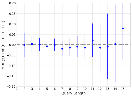
Figure 2. MRR@10 difference between BECR and BECR^-, and 95% confidence interval by query length on MS MARCO Dev

4.3. Different Design Options for BECR

RQ3. Impact of query decomposition and embedding composition by query lengths. Using pre-computed token embeddings for a query would reduce the contextual information that the ranker learns from the query, and we investigate to what extent it affects ranking performance based on different query lengths. We use the MS MARCO Dev set to compare BECR with BECR^- because this set has a large number of queries with diverse lengths. Figure 2 shows the MRR metric difference between BECR and BECR^- segmented by the query length, namely $MRR_{BECR}-MRR_{BECR^{-}}$. The mean value with a dot and the 95% confidence interval are depicted for each query length. For queries with 6 words or less, the BECR model performs similarly as BECR^-, with a 0.0015 drop over 4601 queries in MRR@10, while for the 2379 longer queries from 7 words to 15 words, the average degradation of BECR from BECR^- is 0.0069.

While BECR^- seems to be slightly better than BECR especially for longer queries in relevance, we are not able to confirm this conclusion with statistically significance for this dataset when the query length increases because the 95% confidence interval at each query length overlaps with value 0. Overall, the query decomposition on longer queries has a bigger degradation than it on shorter queries but the degradation is of reasonable magnitude.

Table 4. Relevance of different design options for BECR with different query lengths measured by NDCG@5.

Model	ClueWeb09-Cat-B
Query Length	1	2	3	$\geq 4$	Overall
BECR; no token pairs	0.3399	0.4386	0.3228	0.3349	0.3537
BECR; no uni-gram	–	0.4509	0.3235	0.3638	0.3617
BECR; window=1	0.3407	0.4475	0.3108	0.3499	0.3520
BECR; tokens for Q&D	0.298	0.4104	0.2543	0.2818	0.3034
BECR	0.3407	0.4475	0.3250	0.3717	0.3628

Table 5. NDCG results after removing a scoring component. Statistical significant degradation from BECR at confidence level 95% is marked with ^$.

Model	ClueWeb09-Cat-B
NDCG@k	3 ($\Delta\times 100$)	5 ($\Delta\times 100$)	10 ($\Delta\times 100$)
BECR	0.3754	0.3632	0.3417
No $S_{deep}$	0.2915 (-8.4)$	0.2948 (-6.8)$	0.2788 (-6.3)$
No $S_{lexi}$	0.2673 (-10.8)$	0.2643 (-9.9)$	0.2561 (-8.6)$
No $S_{others}$	0.3099 (-6.5)$	0.3032 (-6.0)$	0.2922 (-5.0)$

Other design options. Table 8 compares other design options for BECR when the number of query words varies in ClueWeb09-Cat-B. The row marked with “BECR; no token pairs” means online query representation is derived only based on uni-grams. This is the extreme case where the weights on all token pairs are 0. BECR outperforms this variation visually for the overall NDCG@5 score, and especially for longer queries in this case. This shows that the use of token pair encoding to approximate query representation brings a visible advantage. On the other hand, this result shows that when the embeddings of word-pair tokens are not available, BECR can resort to rely on uni-gram embeddings to compose the query representation.

The row marked with “BECR; no uni-gram” means online query representation is derived only based on token pairs, and the weights on uni-grams are 0. BECR has a comparable relevance in this case, meaning the use of uni-gram embeddings does not bring a significantly advantage. This is intuitive as the word-pair embeddings contains the meaning of uni-grams. However as stated above, the use of uni-grams is still meaningful especially when the embeddings for some word pairs are not pre-computed.

The row marked with “BECR; window=1” means we only consider uni-gram and adjacent query word pairs in the encoding. By comparing the result of it with $BECR$ on longer queries (column $3$ or $\geq 4$), we can see that incorporating the nonadjacent word pairs seem to help improve the quality of query representations.

Lastly, the row marked with “BECR; tokens for Q&D” represents a case where both the query and the document are encoded using pre-computed uni-gram and word-pair embeddings during inference time. The model relevance drops significantly, indicating that document embeddings directly composed from pre-computed token embeddings are less effective.

RQ4. Table 5 reports the NDCG results after removing one of scoring components to demonstrate the contribution of each component in ClueWeb09-Cat-B. Taking BECR as baseline, for each model variation after removing a component, we report the NDCG results with the NDCG degradation $\Delta$ multiplied by 100. Statistical significant degradation from BECR at confidence level 95% is marked with ^$. For example, for Row marked with “No $S_{deep}$”, it means the model trained without the deep soft contextual matching component and there is a 6.3 point drop in NDCG@10. The results for the other datasets have a similar pattern.

From Row“No $S_{lexi}$”, the removal of $S_{lexi}$ causes relevance degradation by 10.8, 9.9, and 8.6 points for NDCG@3, NDCG@5, and NDCG@10, respectively in ClueWeb09-Cat-B. For the other datasets, we observe a 3% degradation on Robust04 and a 5%-7% drop on the MS MARCO Dev and TREC DL datasets. Thus, adding the lexical component into BECR brings benefits for both document and passage re-ranking. BECR relies more on $S_{lexi}$ for ClueWeb09-Cat-B, probably because the content of web data is more diversified with mixed qualities, and there are more matched documents for each query.

The removal of $S_{others}$ causes a noticable degradation of NDCG results for ClueWeb09-Cat-B. That is because $S_{others}$ contains the pagerank score, which is a very useful document quality signal.

RQ5. We evaluate the tradeoff between storage reduction and relevance with LSH and compact layer choices of BERT. Table 6 shows the NDCG relevance score and storage space requirement for different LSH encoding size and the number of layers used for ClueWeb09-Cat-B which has more and longer documents than the other tested datasets. From the table we can see that by LSH encoding with 256-bit footprint and using 5 layers in training and inference, we are able to reduce the document storage to $0.4\%$ of the original space while achieving comparable ranking performance.

Table 6. Relevance (drop in percentage) and storage tradeoff (ClueWeb09-Cat-B). Significant drop from original L=13 at confidence level 95% is marked with ^$.

LSH bit		NDCG@k			Storage
b	L	3	5	10	D(TB)	Q(TB)
Original	13	0.3754	0.3632	0.3417	1711	37.9
512	13	-2.5%	-0.9%	-1.5%	35.8	0.79
256	13	+0.4%	-0.9%	+0.2%	17	0.39
128	13	-8.9%$	-6.2%	-3.9%	9.1	0.20
64	13	-12%$	-9.8%$	-5.7%	4.6	0.10
32	13	-17.3%$	-13.6%$	-11.5% $	2.4	0.05
Original	5	0.3672	0.3595	0.3375	658.1	14.6
256	5	-2.7%	-1.4%	-3.2%	7.0	0.15
Original	1	0.3348$	0.3263$	0.3112$	76.9	1.36
256	1	-0.3% $	-0.0% $	-0.0% $	1.5	0.03

5. Concluding Remarks

The main contribution of this work is to show how a lightweight BERT based re-ranking model for top results with decent relevance can be made possible to deliver fast response time on affordable computing platforms. Our evaluation shows that its inference time using C++ on a CPU server without GPU is as fast as tens of milliseconds for the ClueWeb09 dataset while the access to an embedding store incurs a modest time cost. With composite token encoding, BECR effectively approximates the query representations and makes a use of both deep contextual and lexical matching features, allowing for a reasonable tradeoff between ad-hoc ranking relevance and efficiency.

There are opportunities for additonal improvement as future work. For example, the disk access cost to fetch precomputed embeddings still takes a significant amount of time compared to the reduced ranking inference time, and when there is a large number of queries processed simultaneously, disk I/O contention can arise. Thus further embedding storage optimization is desirable.

Acknowledgments. We thank Mayuresh Anand, Shiyu Ji, Yang Yang, and anonymous referees for their valuable comments and/or help. This work is supported in part by NSF IIS-2040146 and by a Google faculty research award. It has used the Extreme Science and Engineering Discovery Environment (Towns et al., 2014) supported by NSF ACI-1548562. Any opinions, findings, conclusions or recommendations expressed in this material are those of the authors and do not necessarily reflect the views of the NSF.

Appendix A Additional evaluation information

Data. The data collections used are summarized in Table 7. 1) Robust04 uses TREC Disks 4 & 5 (excluding Congressional Records). Note that we used title queries for the reported experiments. To train the model, we split the queries into five folds based on (Huston and Croft, 2014), with three folds used for training, one for validation, and one for testing. 2) ClueWeb09-Cat-B uses ClueWeb09 Category B with 50M web pages. There are 200 topic queries from the TREC Web Tracks 2009 to 2012. After removing one query with 10 terms, the lengths of queries range from 1 to 5. Spam filtering is applied on ClueWeb09 Category B using Waterloo spam score  with threshold 60. To ensure enough samples in training phase, we add the 50 queries from 2012 in all the five training folds. For the 150 queries from 2009 to 2011, we split the queries into five folds based on (Huston and Croft, 2014). 3) The MS MARCO passage ranking dataset collects the passages from Bing search logs, consisting of 8.8 million passages and over 50 thousand queries with relevance labels. Our evaluation also uses TREC DL 2019 and 2020 from MS MARCO as they have more comprehensive relevance judgements.

Table 7. Summary of Evaluation Data

Dataset	Domain	# Query	# Doc	Query Length	Mean Doc Length
ClueWeb09	Web	149	50M	1-5	857
Robust04	News	250	0.5M	1-4	479
MS MARCO Dev	Q&A, passage	6980	8.8M	2-15	57
TREC DL19	Q&A, passage	43	–	2-15	–
TREC DL20	Q&A, passage	54	–	2-15	–

Non-neural features. Table 8 lists the non-neural features used in our three-dataset evaluation. Feature “tfidf in X” means the TFIDF score of each query token in X where X is either body or title. Feature “bm25 in X” means the BM25 score of each query token in X. Feature “inv_min_dist in X” means the inverse of the smallest distance between any pair of query tokens in X. The prefix max, min, avg and sum mean the maximum, minimum, average or sum of the corresponding feature values for all query tokens.

Table 8. Non-neural features used in the evaluation

Feature name	Note
max tfidf in title	not in MS MARCO passage
min tfidf in title
avg tfidf in title
sum tfidf in title
max tfidf in body
min tfidf in body
avg tfidf in body
sum tfidf in body
sum tfidf in body and title	not in MS MARCO passage
max bm25 in title	not in MS MARCO passage
min bm25 in title
avg bm25 in title
sum bm25 in title
max bm25 in body
min bm25 in body
avg bm25 in body
sum bm25 in body
sum bm25 in body and title	not in MS MARCO passage
max inv_min_dist in title	not in MS MARCO passage
min inv_min_dist in title
avg inv_min_dist in title
max inv_min_dist in body
min inv_min_dist in body
avg inv_min_dist in body
pageRank	only available in Clueweb09

Appendix B An example of ranking with BECR

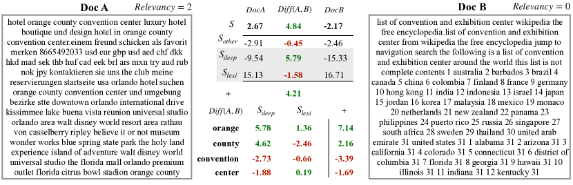
Figure 3. Score difference and breakdown of two matched documents for Query ”orange county convention center”

This section gives an example to rank two documents for a query with BECR and illustrates its component scores in Figure 3. Taking advantage of linear composition, we use the score and subscore difference to understand feature contribution in comparing the document rank order. Both the query and documents are from the ClueWeb09-Cat-B dataset. The query is orange county convention center. Document $A$ is judged as relevant while Document $B$ is not, and BECR gives a higher final rank score to Document A. Based on the text of documents, Document $A$ is about hotel information near Orange county convention center while Document $B$ is a Wikipedia article with a list of convention and exhibit centers.

The middle of Figure 3 depicts the score differences of these two documents. The overall score of Document A as 2.67 is higher than that of Document B. The dominating reason is that $S_{deep}$ deep soft matching score of $A$ is much higher than that of $B$ even the lexical component score of $A$ is slightly lower than $B$. That can be observed by looking at the largest difference in the $Diff(A,B)$ column.

To further understand why Document $A$ matches better semantically for this query, we further show the subscore breakdown of soft and lexical matchings for the token interaction level in the bottom table. The column under $S_{deep}$ shows the difference breakdown $Diff(A,B)$ for component $S_{deep}$ under each query token word. while the column under $S_{lexi}$ shows the difference breakdown for $S_{lexi}$. The last column under $+$ contains the sum of the difference under each token by adding up the soft and lexical matching subscores. We can see that Document $A$ matches the query better because it has more information regarding orange county, although Document $B$ matches with convention center better. Token orange is not mentioned at all in Document $B$ and this is the reason that both soft and lexical matching prefers Document $A$. For token county, Document $B$ has a higher lexical matching subscore because that term occurs several times in Document $B$.

The PageRank score is 4.69 for document $A$ and 6.77 for Document $B$. The weight of PageRank feature learned by BECR is 0.044. Based on linearity, PageRank feature contribute 0.92 ($0.044*(6.77-4.69)=0.92$) to the score difference (both $S_{others}$ and $S$) between Doc A and Doc B. It is not sufficient to outweigh the difference caused by soft matching.

References

- (1)
- Bai et al. (2008) Jing Bai, Yi Chang, Hang Cui, Zhaohui Zheng, Gordon Sun, and Xin Li. 2008. Investigation of partial query proximity in web search. In WWW.
- Bond (2020) Conor Bond. 2020. 27 Google Search Statistics You Should Know in 2019. https://www.wordstream.com/blog/ws/2019/02/07/google-search-statistics.
- Boytsov and Kolter (2021) Leonid Boytsov and Zico Kolter. 2021. Exploring Classic and Neural Lexical Translation Models for Information Retrieval: Interpretability, Effectiveness, and Efficiency Benefits. In ECIR 2021, Vol. 12656. Springer, 63–78.
- Chen et al. (2020) Jiecao Chen, Liu Yang, Karthik Raman, Michael Bendersky, Jung-Jung Yeh, Yun Zhou, Marc Najork, D. Cai, and Ehsan Emadzadeh. 2020. DiPair: Fast and Accurate Distillation for Trillion-Scale Text Matching and Pair Modeling. In EMNLP.
- Choi et al. (2021) Jaekeol Choi, Euna Jung, J. Suh, and Wonjong Rhee. 2021. Improving Bi-encoder Document Ranking Models with Two Rankers and Multi-teacher Distillation. SIGIR (2021).
- Dai and Callan (2019) Zhuyun Dai and J. Callan. 2019. Deeper Text Understanding for IR with Contextual Neural Language Modeling. SIGIR (2019).
- Dai and Callan (2020) Zhuyun Dai and J. Callan. 2020. Context-Aware Document Term Weighting for Ad-Hoc Search. Proceedings of The Web Conference 2020 (2020).
- Dai et al. (2018) Zhuyun Dai, Chenyan Xiong, Jamie Callan, and Zhiyuan Liu. 2018. Convolutional neural networks for soft-matching n-grams in ad-hoc search. In WSDM. ACM, 126–134.
- Devlin et al. (2019) J. Devlin, Ming-Wei Chang, Kenton Lee, and Kristina Toutanova. 2019. BERT: Pre-training of Deep Bidirectional Transformers for Language Understanding. In NAACL-HLT.
- Gao et al. (2020a) Luyu Gao, Zhuyun Dai, and Jamie Callan. 2020a. Modularized Transfomer-based Ranking Framework. In EMNLP.
- Gao et al. (2020b) Luyu Gao, Zhuyun Dai, Zhen Fan, and J. Callan. 2020b. Complementing Lexical Retrieval with Semantic Residual Embedding. ArXiv abs/2004.13969 (2020).
- Guo et al. (2016) J. Guo, Y. Fan, Qingyao Ai, and W. Croft. 2016. A Deep Relevance Matching Model for Ad-hoc Retrieval. CIKM (2016).
- Guthrie et al. (2006) David Guthrie, Ben Allison, Wei Liu, Louise Guthrie, and Yorick Wilks. 2006. A Closer Look at Skip-gram Modelling. European Language Resources Association (ELRA), Genoa, Italy.
- Hofstätter et al. (2021) Sebastian Hofstätter, Bhaskar Mitra, Hamed Zamani, Nick Craswell, and A. Hanbury. 2021. Intra-Document Cascading: Learning to Select Passages for Neural Document Ranking. SIGIR (2021).
- Hofstätter et al. (2020a) Sebastian Hofstätter, Hamed Zamani, Bhaskar Mitra, Nick Craswell, and A. Hanbury. 2020a. Local Self-Attention over Long Text for Efficient Document Retrieval. SIGIR (2020).
- Hofstätter et al. (2020b) Sebastian Hofstätter, Markus Zlabinger, and A. Hanbury. 2020b. Interpretable & Time-Budget-Constrained Contextualization for Re-Ranking. In ECAI.
- Humeau et al. (2020) Samuel Humeau, Kurt Shuster, Marie-Anne Lachaux, and J. Weston. 2020. Poly-encoders: Architectures and Pre-training Strategies for Fast and Accurate Multi-sentence Scoring. In ICLR.
- Huston and Croft (2014) S. Huston and W. Croft. 2014. A Comparison of Retrieval Models using Term Dependencies. CIKM (2014).
- Jansen and Spink (2006) Bernard J Jansen and Amanda Spink. 2006. How are we searching the World Wide Web? A comparison of nine search engine transaction logs. Information processing & management 42, 1 (2006), 248–263.
- Järvelin and Kekäläinen (2002) Kalervo Järvelin and Jaana Kekäläinen. 2002. Cumulated gain-based evaluation of IR techniques. ACM Transactions on Information Systems (TOIS) 20, 4 (2002), 422–446.
- Ji et al. (2019) Shiyu Ji, Jinjin Shao, and Tao Yang. 2019. Efficient Interaction-based Neural Ranking with Locality Sensitive Hashing. In WWW (San Francisco, CA, USA). ACM, New York, NY, USA, 2858–2864.
- Jiang et al. (2020) Jyun-Yu Jiang, Chenyan Xiong, Chia-Jung Lee, and W. Wang. 2020. Long Document Ranking with Query-Directed Sparse Transformer. In FINDINGS.
- Jones et al. (2000) Karen Spärck Jones, Steve Walker, and Stephen E. Robertson. 2000. A probabilistic model of information retrieval: development and comparative experiments. In Information Processing and Management. 779–840.
- Karpukhin et al. (2020) V. Karpukhin, Barlas Oğuz, Sewon Min, Patrick Lewis, Ledell Yu Wu, Sergey Edunov, Danqi Chen, and Wen tau Yih. 2020. Dense Passage Retrieval for Open-Domain Question Answering. ArXiv abs/2010.08191 (2020).
- Khattab and Zaharia (2020) O. Khattab and M. Zaharia. 2020. ColBERT: Efficient and Effective Passage Search via Contextualized Late Interaction over BERT. SIGIR (2020).
- Kingma and Ba (2015) Diederik P. Kingma and Jimmy Ba. 2015. Adam: A Method for Stochastic Optimization. CoRR abs/1412.6980 (2015).
- Li et al. (2020) Canjia Li, A. Yates, Sean MacAvaney, B. He, and Yingfei Sun. 2020. PARADE: Passage Representation Aggregation for Document Reranking. ArXiv abs/2008.09093 (2020).
- Lin et al. (2020) Jimmy Lin, Rodrigo Nogueira, and A. Yates. 2020. Pretrained Transformers for Text Ranking: BERT and Beyond. ArXiv abs/2010.06467 (2020).
- Liu (2010) T. Liu. 2010. Learning to rank for information retrieval. In SIGIR ’10.
- Lu et al. (2020) Wenhao Lu, Jian Jiao, and Ruofei Zhang. 2020. TwinBERT: Distilling Knowledge to Twin-Structured BERT Models for Efficient Retrieval. ArXiv abs/2002.06275 (2020).
- Luan et al. (2020) Yi Luan, Jacob Eisenstein, Kristina Toutanova, and M. Collins. 2020. Sparse, Dense, and Attentional Representations for Text Retrieval. ArXiv abs/2005.00181 (2020).
- MacAvaney et al. (2020a) Sean MacAvaney, F. Nardini, R. Perego, N. Tonellotto, Nazli Goharian, and O. Frieder. 2020a. Efficient Document Re-Ranking for Transformers by Precomputing Term Representations. SIGIR (2020).
- MacAvaney et al. (2020b) Sean MacAvaney, F. M. Nardini, R. Perego, N. Tonellotto, Nazli Goharian, and O. Frieder. 2020b. Expansion via Prediction of Importance with Contextualization. SIGIR (2020).
- MacAvaney et al. (2019) Sean MacAvaney, Andrew Yates, Arman Cohan, and Nazli Goharian. 2019. CEDR: Contextualized Embeddings for Document Ranking. SIGIR (2019).
- Mikolov et al. (2013) Tomas Mikolov, Ilya Sutskever, Kai Chen, G. S. Corrado, and J. Dean. 2013. Distributed Representations of Words and Phrases and their Compositionality. ArXiv abs/1310.4546 (2013).
- Mitra et al. (2017) Bhaskar Mitra, F. Diaz, and Nick Craswell. 2017. Learning to Match using Local and Distributed Representations of Text for Web Search. WWW (2017).
- Mitra et al. (2020) Bhaskar Mitra, Sebastian Hofstätter, Hamed Zamani, and Nick Craswell. 2020. Conformer-Kernel with Query Term Independence for Document Retrieval. ArXiv abs/2007.10434 (2020).
- Nogueira and Cho (2019) Rodrigo Nogueira and Kyunghyun Cho. 2019. Passage Re-ranking with BERT. ArXiv abs/1901.04085 (2019).
- Nogueira et al. (2020) Rodrigo Nogueira, Zhiying Jiang, Ronak Pradeep, and Jimmy Lin. 2020. Document Ranking with a Pretrained Sequence-to-Sequence Model. In Findings of the Association for Computational Linguistics: EMNLP 2020.
- Nogueira et al. (2019) Rodrigo Nogueira, W. Yang, Kyunghyun Cho, and Jimmy Lin. 2019. Multi-Stage Document Ranking with BERT. ArXiv abs/1910.14424 (2019).
- Reimers and Gurevych (2019) Nils Reimers and Iryna Gurevych. 2019. Sentence-BERT: Sentence Embeddings using Siamese BERT-Networks. In EMNLP/IJCNLP.
- Shao et al. (2019) Jinjin Shao, Shiyu Ji, and Tao Yang. 2019. Privacy-aware Document Ranking with Neural Signals. SIGIR (2019).
- Soldaini and Moschitti (2020) Luca Soldaini and Alessandro Moschitti. 2020. The Cascade Transformer: an Application for Efficient Answer Sentence Selection. ArXiv abs/2005.02534 (2020).
- Sun et al. (2021) Si Sun, Yingzhuo Qian, Zhenghao Liu, Chenyan Xiong, Kaitao Zhang, Jie Bao, Zhiyuan Liu, and Paul N. Bennett. 2021. Few-Shot Text Ranking with Meta Adapted Synthetic Weak Supervision. In ACL/IJCNLP.
- Towns et al. (2014) J. Towns, T. Cockerill, M. Dahan, I. Foster, K. Gaither, A. Grimshaw, V. Hazlewood, S. Lathrop, D. Lifka, G. D. Peterson, R. Roskies, J. Scott, and N. Wilkins-Diehr. 2014. XSEDE: Accelerating Scientific Discovery. Computing in Science & Engineering 16, 05 (2014), 62–74.
- Wu et al. (2016) Y. Wu, M. Schuster, Z. Chen, Quoc V. Le, M. Norouzi, W. Macherey, M. Krikun, Y. Cao, Q. Gao, K. Macherey, J. Klingner, A. Shah, M. Johnson, X. Liu, L. Kaiser, S. Gouws, Y. Kato, T. Kudo, H. Kazawa, K. Stevens, G. Kurian, N. Patil, W. Wang, C. Young, J. Smith, J. Riesa, A. Rudnick, O. Vinyals, G. S. Corrado, M. Hughes, and J. Dean. 2016. Google’s Neural Machine Translation System: Bridging the Gap between Human and Machine Translation. ArXiv abs/1609.08144 (2016).
- Xin et al. (2020) J. Xin, Rodrigo Nogueira, Y. Yu, and Jimmy Lin. 2020. Early Exiting BERT for Efficient Document Ranking. In SUSTAINLP.
- Xiong et al. (2017) Chenyan Xiong, Zhuyun Dai, J. Callan, Zhiyuan Liu, and R. Power. 2017. End-to-End Neural Ad-hoc Ranking with Kernel Pooling. SIGIR (2017).
- Yang et al. (2019) Wei Yang, Haotian Zhang, and Jimmy Lin. 2019. Simple Applications of BERT for Ad Hoc Document Retrieval. ArXiv abs/1903.10972 (2019).
- Yilmaz et al. (2019) Zeynep Akkalyoncu Yilmaz, W. Yang, Haotian Zhang, and Jimmy J. Lin. 2019. Cross-Domain Modeling of Sentence-Level Evidence for Document Retrieval. In EMNLP/IJCNLP.
- Zafrir et al. (2019) Ofir Zafrir, Guy Boudoukh, Peter Izsak, and Moshe Wasserblat. 2019. Q8BERT: Quantized 8Bit BERT. In 5th Workshop on Energy Efficient Machine Learning and Cognitive Computing - NeurIPS 2019.
- Zhan et al. (2020a) Jingtao Zhan, J. Mao, Yiqun Liu, Min Zhang, and Shaoping Ma. 2020a. Learning To Retrieve: How to Train a Dense Retrieval Model Effectively and Efficiently. ArXiv abs/2010.10469 (2020).
- Zhan et al. (2020b) Jingtao Zhan, Jiaxin Mao, Yiqun Liu, Min Zhang, and Shaoping Ma. 2020b. RepBERT: Contextualized Text Embeddings for First-Stage Retrieval. ArXiv abs/2006.15498 (2020).
- Zhang et al. (2020b) Kaitao Zhang, Chenyan Xiong, Zhenghao Liu, and Zhiyuan Liu. 2020b. Selective Weak Supervision for Neural Information Retrieval. WWW (2020).
- Zhang et al. (2020c) Xinyu Zhang, Andrew Yates, and Jimmy J. Lin. 2020c. A Little Bit Is Worse Than None: Ranking with Limited Training Data. In SUSTAINLP.
- Zhang et al. (2020a) Y. Zhang, Ping Nie, Xiubo Geng, A. Ramamurthy, L. Song, and Daxin Jiang. 2020a. DC-BERT: Decoupling Question and Document for Efficient Contextual Encoding. In SIGIR.
- Zhao and Huang (2014) Jiashu Zhao and Jimmy Xiangji Huang. 2014. An Enhanced Context-sensitive Proximity Model for Probabilistic Information Retrieval. In SIGIR. 1131–1134.
- Zhuang et al. (2020) Honglei Zhuang, Xuanhui Wang, Mike Bendersky, Alexander Grushetsky, Yonghui Wu, Petr Mitrichev, E. Sterling, N. Bell, Walker Ravina, and H. Qian. 2020. Interpretable Learning-to-Rank with Generalized Additive Models. ArXiv abs/2005.02553 (2020).
- Zhuang and Zuccon (2021) Shengyao Zhuang and G. Zuccon. 2021. TILDE: Term Independent Likelihood moDEl for Passage Re-ranking. SIGIR (2021).