ON SYNTHETIC ABSORPTION LINE PROFILES OF THERMALLY DRIVEN WINDS FROM ACTIVE GALACTIC NUCLEI

Abstract

The warm absorbers observed in more than half of all nearby active galactic nuclei (AGN) are tracers of ionized outflows located at parsec scale distances from the central engine. If the smallest inferred ionization parameters correspond to plasma at a few $10^{4}$ K, then the gas undergoes a transition from being bound to unbound provided it is further heated to $\sim 10^{6}$ K at larger radii. Dannen et al. recently discovered that under these circumstances, thermally driven wind solutions are unsteady and even show very dense clumps due to thermal instability. To explore the observational consequences of these new wind solutions, we compute line profiles based on the one-dimensional simulations of Dannen et al.. We show how the line profiles from even a simple steady state wind solution depend on the ionization energy (IE) of absorbing ions, which is a reflection of the wind ionization stratification. To organize the diversity of the line shapes, we group them into four categories: weak Gaussians, saturated boxy profiles with and without an extended blue wing, and broad weak profiles. The lines with profiles in the last two categories are produced by ions with the highest IE that probe the fastest regions. Their maximum blueshifts agree with the highest flow velocities in thermally unstable models, both steady state and clumpy versions. In contrast, the maximum blueshifts of the most high IE lines in thermally stable models can be less than half of the actual solution velocities. Clumpy solutions can additionally imprint distinguishable absorption troughs at widely separated velocities.

1 Introduction

Seyfert galaxies generally display absorption lines with relatively small blueshifts ($\sim$ 100 –1000 km s^-1) in their UV and X-ray spectra, indicating the presence of mass outflows (Reynolds, 1997; Crenshaw et al., 1999). In some such galaxies, the X-ray absorbers (the so-called warm absorbers, WAs) and UV absorbers have very similar velocities which suggests that these absorbers are nearly cospatial. This, in turn, suggests that regions of very different temperatures coexist and that the absorption occurs in a multi-phase outflow (e.g., Shields & Hamann, 1997; Crenshaw et al., 1999; Gabel et al., 2003; Longinotti et al., 2013; Ebrero et al., 2016; Fu et al., 2017; Mehdipour et al., 2017, and references therein).

Mass outflows with relatively small velocities such as these could be thermally driven winds launched at large distances from the central engine of an active galactic nuleus (AGN). There are a few plausible origins for these distant outflows: (1) a parsec-scale Compton-heated disk wind (e.g., Begelman et al., 1983; Woods et al., 1996; Waters et al., 2021); (2) a wind blown from the inner regions of a torus of dusty material (e.g. Balsara & Krolik, 1993; Dorodnitsyn et al., 2008a, b, 2012, 2016; Kallman & Dorodnitsyn, 2019); (3) an outflow driven directly from gas infalling towards an SMBH (e.g., Proga, 2007; Proga et al., 2008; Kurosawa & Proga, 2009a, b); and (4) a quasi-spherical outflow driven from an even simpler structure such as a static (non-rotationally supported) shell of gas (e.g., Everett & Murray, 2007).

A basic challenge faced by any theoretical model is whether it can account for both the velocity and ionization range inferred from observations. The calculations by Sim et al. (2012), who computed spectra based on the initial, exploratory simulations from Kurosawa & Proga (2009a), illustrate the difficulties typically encountered. They found that while the outflow velocities are roughly consistent with observations, the column density and ionization state of the outflowing gas are too high in the models. As such, type (3) models are unlikely to account for WAs, which are often observed in AGNs when there is sufficient sensitivity to detect them (Reynolds, 1997; Blustin et al., 2005; Ricci et al., 2017; McKernan et al., 2007; Laha et al., 2014).

Sim et al. (2012) discussed a few changes to type (3) models that could reduce the discrepancy between the model predictions and the observations. While a global change of the gas density or X-ray flux is always a possibility, they noted that it might be more promising to have smaller scale changes in the structure of the outflowing gas. For a similar total mass outflow rate, higher density might be achieved if it were more strongly clumped. Such a change would not only lead to lower ionization but could also reduce the column density because smaller clumps would subtend smaller solid angles as seen by the central source. Similar conclusions were later reached by Mizumoto et al. (2019) in the case of type (1) models. Very recently, Waters et al. (2021) showed that multi-phase versions of type (1) solutions do exist. They found that sight lines probing clumps can indeed provide the necessary low ionization gas column density, while their synthetic line profile calculations showed interesting differences between high ionization and low ionization X-ray lines.

The work of Waters et al. (2021) represents our latest effort to understand how X-ray irradiation can trigger thermal instability (TI, Field, 1965) in global dynamical flows. Once TI operates, the denser, cooler gas inferred to be necessary to account for the observed ionization states of WAs can naturally be produced. The first breakthrough in this line of modeling work came while modeling irradiated inflows. Namely, it was shown how the in situ production of multi-phase gas can be triggered using global time-dependent hydrodynamical simulations of Bondi-like accretion flows (e.g., Proga et al., 2008; Kurosawa & Proga, 2009a, b; Barai et al., 2012; Mościbrodzka & Proga, 2013; Gaspari et al., 2013; Takeuchi et al., 2013). In an outflow regime akin to type (4) models, Dannen et al. (2020, hereafter D20) recently demonstrated that thermally driven outflow solutions can also become clumpy due to TI for a certain range of parameters.

In this paper, we explore the observational consequences of this new type (4) model, which is an easily reproducible example of a multi-phase thermally driven radial AGN outflow. Specifically, here we present line profile calculations for global simulations that capture the dynamics of smooth flows as well as clumpy outflows as they expand and transition back into a smooth flow. Our aim here is two-fold: (i) understanding line profiles from 1D spherically symmetric solutions before performing similar studies for multi-dimensional models and (ii) assessing if these simple solutions are themselves a promising model of WAs. Our first aim is related to checking if simple 1D models produce simple line profiles for all ions or whether they produce a complex and diverse class of profiles.

This paper is organized as follows. In section 2, we present all the models analysed in this work. In section 3, we summarize our methods of calculating synthetic line profiles for these models. In section 4 and 5, we present the results of our line profile calculations and our discussion.

Table 1: Model parameters and some gross properties of steady wind models A21, B and C. These models share the following basic parameters: $\Gamma=0.3$, $\Xi_{0}=3.12$ ($\xi_{0}=5.0$ erg cm s^-1) and $M_{\rm BH}=10^{6}M_{\odot}$.

Model	HEP0	$r_{0}$	$\rho_{0}$	$v$	$\dot{M}$	$r_{\rm out}$	$N_{H}$
		[$10^{18}$ cm]	[$10^{-18}$ g cm-3]	[km s-1]	[$10^{24}$ g s-1]	[$10^{18}$ cm]	[$10^{23}$ cm-2]
A21	14.7	0.91	3.28	659.3	1.1	9.14	1.22
B	11.9	1.13	2.15	346.0	3.4	11.28	1.47
C	9.1	1.48	1.25	248.0	6.1	14.76	1.35

Note. — D20 found that models B and C are unsteady. However, Waters et al. (2021) refined the numerical methods and found that these two models can eventually settle down to an unstable yet steady state. Once these solutions are perturbed they become clumpy in agreement with D20’s findings. The second, third, and fourth columns list the hydrodynamic escape parameter $\rm{HEP}_{0}$, the inner radius $r_{0}$, and the density $\rho_{0}$ at $r_{0}$, respectively. The next three columns list the following properties of the solutions: the flow velocity $v$ and mass loss rate $\dot{M}$ at the outer most grid point, $r_{\rm out}$, at a late time when the flow has become steady. The last column shows the hydrogen column density $N_{H}$ for the outflow.

2 Models

Using the magnetohydrodynamics code Athena++ (Stone et al., 2020), D20 solved the equations of non-adiabatic gas dynamics with a radiation force due to electron scattering for an unobscured AGN SED (that of NGC 5548; see Mehdipour et al., 2015). The line force in these warm/hot winds can exceed gravity but it is much weaker than the gas pressure force (Dannen et al., 2019), and has therefore been ignored in D20 for simplicity. They explored a parameter space comprised of the three dimensionless parameters governing thermal wind solutions: (1) Eddington fraction, $\Gamma$ (=$L/L_{\rm Edd}$ for a system with luminosity $L$), which sets the radiation force per unit volume due to electron scattering as $F_{\rm rad}=GM_{\rm BH}\rho\,\Gamma/r^{2}$ ($M_{\rm BH}$ is the black hole mass and $\rho$ the gas density at radius $r$), (2) the pressure ionization parameter at the base of the wind, $r_{0}$,

$$\Xi_{0}=\frac{p_{\rm rad}}{p}\biggr{\rvert}_{r=r_{0}}=\frac{\xi_{0}}{4\pi ck_{B}T_{0}},$$ (1)

where $p_{\rm rad}=F_{X}/c=f_{X}\Gamma L_{\rm Edd}/(4\pi r^{2}c)$ is the radiation pressure, $f_{X}\equiv L_{X}/L$ is the ionizing portion of the SED ($f_{X}=0.36$ for the NGC 5548 SED used by D20), and $\xi_{0}=L_{X}/(n_{0}r_{0}^{2})$ is the density ionization parameter (with $n_{0}=\rho_{0}/\bar{m}$, $\bar{m}$ being the mean molecular mass), and (3) the hydrodynamic escape parameter evaluated at $r_{0}$, $\rm{HEP}_{0}$. This parameter is defined as the ratio of effective gravitational potential and thermal energy at $r_{0}$,

$$\rm{HEP}_{0}\equiv\frac{GM_{\rm BH}(1-\Gamma)}{r_{0}c_{\rm s,0}^{2}},,$$ (2)

where $c_{\rm s,0}=\sqrt{\gamma kT_{0}/\bar{m}}$ is the adiabatic sound speed of the gas with the temperature, $T=T_{0}$, and $\gamma$ is adiabatic index assumed to be 5/3.

To specify the lower boundary conditions of the hydrodynamical simulations (i.e., $T_{0}$, $r_{0}$, and $\rho_{0}$), D20 took the following five steps: (i) selected which SED to use along with its associated ‘S-curve’ and $f_{X}$, (ii) chose values of $M_{\rm BH}$, $\Gamma$, and $\xi_{0}$, (iii) computed $T_{0}$ for the value of $\xi_{0}$ and assuming that the gas is in thermal equilibrium, i.e., $T_{0}=T_{\rm gas}=T_{\rm eq}(\xi_{0})$, (iv) used $T_{0}$ to compute $c_{s,0}$ and then used eq. 2 to obtain the value of $r_{0}$, and finally (v) computed $\rho_{0}$ using the expression for $\xi_{0}$. Keeping the parameters $M_{\rm BH}$, $\Gamma$ and $\xi_{0}$ fixed, D20 altered only the value of the HEP₀ between the models, which required changing $r_{0}$ and $\rho_{0}$. Note that once $\xi_{0}$ is fixed, $\Xi_{0}$ is fixed as well. In Table 1, we summarize the parameters of three simulations and the gross properties of the corresponding outflow solutions.

An extensive exploration of the parameter space led D20 to arrive at a new category of ‘clumpy’ thermal wind models occurring at sufficiently large radius (small $\rm{HEP}_{0}$), namely, solutions that are unstable to TI. As further shown by Waters et al. (2021), these solutions also reach a steady state and only occur beyond a characteristic ‘unbound’ radius given by

$$R_{\rm u}=\frac{2}{\gamma}\frac{\gamma-1}{\gamma+1}\frac{T_{C}}{T_{\rm c,max}}\,R_{\rm IC}\,(1-\Gamma)\approx 140\,R_{\rm IC}\,(1-\Gamma),$$ (3)

where the second expression is evaluated for $\gamma=5/3$ and for the thermal equilibrium or ‘S-curve’ corresponding to Mehdipour et al. 2015’s SED. The ratio $T_{C}/T_{\rm c,max}=4.68\times 10^{2}$, where $T_{C}$ is the Compton temperature ($\sim 10^{8}$ K), $T_{\rm c,max}=T(\Xi_{\rm c,max})$ ($\Xi_{c,max}$ is the critical $\Xi$ for which the gas enters the lower TI zone), and the Compton radius is $R_{\rm IC}=(10^{18}/T_{\rm C})(M/M_{\odot})$ cm.

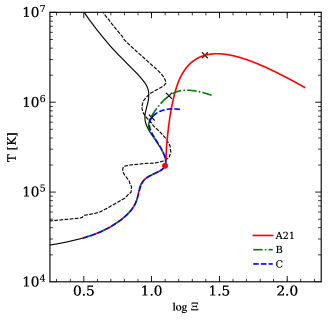
Figure 1: Phase diagram ($T-\Xi$): the solid black line represents the thermal equilibrium curve (S-curve ) while the black dashed line represents the Balbus contour. All points to the left of the latter are thermally unstable whereas those to the right are thermally stable according to Balbus’ criterion for TI (Balbus, 1986). There are two unstable regions encountered while tracing the S-curve starting from low temperatures; we refer to them as the lower and upper TI zones. The figure also shows our three steady wind solutions (solid red, dot-dashed green, and dashed blue line for model A21, B, and C, respectively). We marked the sonic points for each solution with an ‘$\times$’. Notice that upon reaching $\Xi_{\rm c,max}$ (marked by red dot on the S-curve), Model A21 exhibits runaway heating and quickly exits the lower TI zone. Models B and C instead follow the S-curve within this zone. The decrease in temperature beyond the sonic points in all three cases is due to efficient adiabatic cooling being balanced by radiative heating.

In Fig. 1, we show this S-curve (solid black line) along with the Balbus contour (black dashed line) that is necessary to analyze TI in a dynamical flow. Specifically, while regions of negative slope on the S-curve are thermally unstable, the Balbus contour maps out the thermally unstable parameter space both on and off the S-curve, as explained in the caption. These two $T$-$\xi$ relations are computed from our grid of photoionization models first presented in Dyda et al. (2017). In their calculations, Dyda et al. (2017) used version 2.35 of XSTAR (Kallman & Bautista, 2001) and assumed a constant density of $n_{\textrm{\tiny XSTAR}}=10^{8}\,{\rm cm}^{-3}$ over the parameter space with $\log\xi$ in the range -2 – 8, and $T$ in the range $5\times 10^{3}$ – $5\times 10^{8}$ K. We note that, unless otherwise stated, we use cgs units throughout the paper, except for the velocity and distance $(r-r_{0})$, which are in km s^-1 and the inner radius of the computational domain $r_{0}$, respectively.

In this figure, we also present examples of steady state solutions (see the legend for color coding of the curves). The wind solutions chosen are similar to those presented in D20: model A21 is an example of a thermally stable solution, whereas models B and C are examples of thermally unstable solutions. Although all three models reach a time-independent state, they have different properties that signal their stable or unstable character. Namely, after they enter the lower TI zone, the stable solution undergoes rapid heating and leaves the TI zone, evolving under nearly isobaric conditions (moves vertically up on the phase diagram), whereas the unstable solutions continue to follow the S-curve even within the lower TI zone (where the slope of the S-curve is negative) over a relatively wide range of $T$ before they too leave the zone.

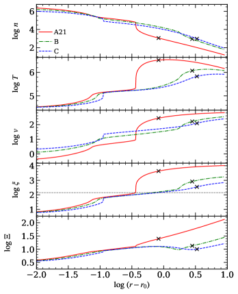
Figure 2: Radial profiles of logarithm of number density $n$ (cm^-3), temperature $T$ (K), flow velocity $v$ (km s^-1), ionization parameter $\xi$ (erg cm s^-1) and the dimensionless pressure ionization parameter $\Xi$, for the three steady wind models shown in Fig. 1. Sonic points are again marked by ‘$\times$’s. The horizontal line in the fourth panel marks $\log(\xi_{\rm c,max})=2.15$, the entry into the lower TI zone.

In Fig. 2, we show radial profiles of the main wind properties of our three steady state solutions. Specifically, we plot the number density $n$, temperature $T$, flow velocity $v$, ionization parameter $\xi$ and the pressure ionization parameter $\Xi$. As discussed above and in D20, model A21 has quite different properties than models B and C. The main reason for this is that model A21 undergoes strong runaway heating (as seen by comparing the temperature profiles), and consequently its velocity/density is higher/lower than that of the other two. In model A21, $\xi$ is also higher than in models B and C. Therefore we can expect that the models will produce spectral lines with different profiles. In general, we also see that $\xi$ increases outward, for all the models. One of our goals is to check how this ionization stratification could be traced in the profiles of absorption lines.

2.1 Clumpy models

Our steady state model A21 is formally stable to TI despite it passing through the lower TI zone in Fig. 1. As discussed by Waters et al. (2021), this happens whenever there is a sharp jump in the entropy profile, which in these solutions will be accompanied by a change in sign of the Bernoulli function. Models B and C, meanwhile, have smooth entropy profiles and the Bernoulli function does not change signs when gas encounters the TI zone. These solutions reach a steady state only when there are no more entropy modes being generated at the base of the flow. Starting from D20’s initial conditions, such entropy modes are only produced for a transient period of time.

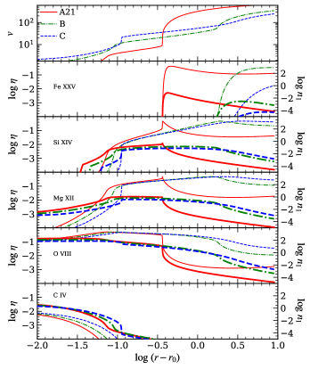
Figure 3: Fractional ionic abundance $\eta$ (shown on left y-axis, with thinner lines) and the ion ground state level population $n_{1}=n\eta A$ (shown on right y-axis, with thicker lines) vs $\log\ (r-r_{0})$, for the same five ions whose line profiles are compared in Fig. 7. The topmost panel shows radial velocity profiles (in $\rm km\,s^{-1}$) to aid in assessing blueshifts. The legend in this panel applies to both the left and right y-axes.

To examine line profiles for clumpy outflow solutions, we reintroduce entropy modes into models B and C to trigger TI. Specifically, isobaric perturbations, i.e. density perturbations applied at constant pressure (and velocity), are added to the wind base by changing the density boundary condition from $\rho_{\rm bc}=\rho_{0}$ to

$$\rho_{\rm bc}(t)=\rho_{0}\left[1+\displaystyle\sum_{m=1}^{m=5}A_{m}\sin\Big{(}\frac{2\pi t}{T_{m}}\Big{)}\right],$$ (4)

where $A_{m}=A_{0}/N_{\rm modes}$ and $T_{m}=mT_{0}$ are the amplitude and period of the driving modes; we set $A_{0}=0.01$ and $T_{0}=t_{dyn}/20$ (where $t_{\rm dyn}=|r/v|$ is the dynamical timescale). We chose this form of density perturbation, comprising five driving modes ($N_{\rm modes}=5)$, as it adequately captures the overall complexity of a clumpy wind solution in a controlled way. We will refer to the perturbed versions of Models B and C as Models B-c and C-c.

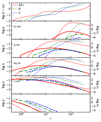
Figure 4: The same quantities in Fig 3 but plotted against the flow velocity $v$ (in $\rm km\,s^{-1}$) rather than distance. The topmost panel shows the radial distribution of $v$.

2.2 Ionization structure and absorption diagnostics

As an aid to understanding our line profile calculations, we examine two other wind properties that enter these calculations, namely the fractional ion abundance, $\eta$, and the level population of the ion’s ground state, $n_{1}=nA\eta$ (where $A$ is the elemental abundance relative to hydrogen). These quantities provide important information about what to expect and/or how to explain the line profile shapes and the presence of the lines themselves. We extract $\eta$ and $n_{1}$ as a part of post-processing from our grid of photoionization calculations from XSTAR. These quantities are related to the line center absorption coefficient contained in XSTAR output,

$$(\kappa_{\nu_{0}}\rho)_{\textrm{\tiny XSTAR}}= \frac{\pi e^{2}}{m_{e}c}n_{1}f_{12}\phi(\nu_{0}),$$

$$= \frac{1}{\sqrt{\pi}}\left[\frac{\pi e^{2}}{m_{e}c}\frac{n_{\textrm{\tiny XSTAR}}A\eta}{\nu_{0}(v_{\text{th}}/c)}f_{12}\right],$$ (5)

where $\kappa_{\nu_{0}}$ is the line center opacity, $\rho=\mu m_{p}n$ is the gas density (mean molecular mass $\mu=0.6$ for this work, $m_{p}$ is the proton mass), $f_{12}$ is the oscillator strength of the lower level of the line, $\phi(\nu)$ is the profile function to be defined later, and $v_{\rm th}(r)=\sqrt{2k_{B}T(r)/m_{i}}$ is the mean thermal velocity of an ion with mass $m_{i}$.

To illustrate the details of the ionization structure, in Figs. 3 and 4, we plot $n_{1}$ for five ions in order of decreasing IE: Fe XXV, Si XIV, Mg XII, O VIII and C IV (plotted on the right y-axis using thicker lines in the second to sixth panels). We also plot $\eta$ along the left y-axis (shown by thinner lines). These two figures are complementary to each other since Fig. 3 shows $n_{1}$ and $\eta$ as functions of radius while Fig. 4 shows these quantities as functions of velocity. This mapping to the velocity space is done solely for the purpose of aiding in our analysis and interpretation of line profile results. To this end, the top panels of Fig. 3 and Fig. 4 show respectively the velocity as a function of distance and the distance as a function of velocity.

The ionization stratification is on full display in these figures, e.g., we see that C IV is only abundant at the wind base whereas Fe XXV only at very large radii. Meanwhile, Si XIV and Mg XII are present at intermediate locations and show up roughly where the C IV abundance drops off. Comparing with Fig. 1 or Fig. 2, we see that C IV disappears at $r>r(\xi_{\rm c,max})$. This is not merely a property of the models but rather the underlying cause explaining why $\xi_{\rm c,max}$ identifies a bend in the S-curve: C IV and other mildly ionized elements provide efficient cooling via line emission, and as these ions rapidly deplete as $\xi$ increases, the photoionization equilibrium temperature must sharply increase as well in order to compensate for this lack of efficient cooling. As we will describe below, this enhanced heating and subsequent gas acceleration results in a drop in the amount of matter (measured by the column density).

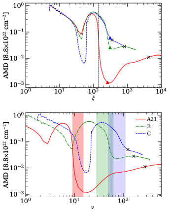
Figure 5: Comparison of the AMD for our three steady state wind solutions. The top panel shows the AMD (eq. 6) in units of its maximum value for model A21 (=$8.8\times 10^{22}{\rm cm}^{-2}$) versus $\xi$. The vertical black dotted line marks the base of the lower TI zone, $\xi=\xi_{c,max}$, while the three triangles mark the points where each model leaves this TI zone. In the bottom panel, these AMDs are mapped onto the flow velocity, $v$ (in km s^-1; the range with $v<1~{}$km s^-1 is not shown). Sonic points are marked with ‘$\times$’ symbols and the color shadings denote the parameter space of gas occupying the lower TI zone.

Our last diagnostic that can help to develop a feel for the absorption properties of our wind solution is the absorption measure distribution (AMD). It is defined as

$${\rm AMD}=\frac{dN_{H}}{d(\log\xi)}=n\lambda_{\xi},$$ (6)

where $N_{H}$ is the hydrogen column density and $\lambda_{\xi}=(d\log{\xi}/dr)^{-1}$ is the characteristic length scale for variations in $\xi$. The AMD has proven to be both an important observable (Holczer et al., 2007; Behar, 2009) and a useful tool for quantifying the absorption properties of hydrodynamical models. We note that for a steady state, $v\propto\xi$ ($v\propto 1/nr^{2}$, as is $\xi$). Therefore, $\lambda_{\xi}=\lambda_{v}\equiv(d\log{v}/dr)^{-1}$.

In Fig. 5, we show the AMDs for our three steady models. There are two prominent dips in the AMD: one at the entrance to the TI zone, which is marked by the vertical line in the top panel, and another at even smaller $\xi$, corresponding to gas on the cold phase branch of the S-curve. The bottom panel in Fig. 5 shows this latter dip occurs for low velocity gas. As pointed out by Dyda et al. (2017), a dip in the AMD can be caused by enhanced heating even in regions that are thermally stable. Referring to Fig. 1, notice that the cold branch of the S-curve becomes nearly vertical (for $\log\Xi\approx 0.9$ and $T$ just above $10^{5}$ K), or equivalently, the S-curve and the Balbus contours approach each other. In this physical regime, the velocity is relatively low but the acceleration is relatively high (e.g., see Fig. 2 for the steep gradient in the radial profiles of $T$, $n$ and $v$). This rapid acceleration leads to the minima in the AMD at $v\approx 2$, 10, and 20 km s^-1 in models A21, B, and C, respectively.

A quantitative understanding of the reason for a decrease in the AMD is found by referring to the right hand side of eq. 6 and noting that $\lambda_{\xi}=\lambda_{v}\equiv(d\log{v}/dr)^{-1}$. Also note that an enhanced acceleration results in shortening the characteristic length scale $\lambda_{v}$. The region of the enhanced acceleration is relatively small. Therefore, $\lambda_{v}$ increases as the slope of the S-curve flattens again, and the AMD recovers to the level from before the drop. Importantly, our analysis above (mentioned while describing Figs. 3 and 4) reveals that such a change in the slope of the S-curve can be driven by a reduction in line cooling: all wind solutions reach this region of enhanced acceleration where the abundance of C IV undergoes a sharp decrease (at $\log(r-r_{0})\approx-1$ in the bottom panel of Fig. 3). In other words, the gas experiences enhanced heating as a result of it losing important coolants.

Farther downstream, the gas becomes even more ionized and, as we already mentioned, it enters the lower TI zone at $\xi_{\rm c,max}$. The corresponding changes in the thermal and dynamical properties of the wind solutions produce a change in the AMD. Namely, the AMD drops by one or even two orders of magnitude (see the shaded color areas in the bottom panel of Fig. 5). This is best exemplified by the results for model A21 where the heating is so enhanced that it leads to runaway heating. The drops in the AMD for models B and C are not as large simply because the heating is weaker. Upon exiting the TI zone, the AMD in model C continues to decrease unlike in models A21 and B where we see a mild increase.

Our analysis demonstrates how the flow properties closely depend on the gas dynamics and thermodynamics even if the flow is time independent. The methodology used by D20 to couple photoionization and hydrodynamical calculations provides us with a substantial amount of information. Not only can we extract the opacities necessary to compute absorption line profiles, but we can also examine intermediate quantities to explain the physics behind the properties of the profiles and the relations between different ionization states.

3 Methods

The photoionization calculations from XSTAR provide us with the quantity in brackets in equation (5) above, for $n=n_{\textrm{\tiny XSTAR}}=10^{8}$ cm^-3. Due to $(\kappa_{\nu_{0}}\rho)_{\textrm{\tiny XSTAR}}$ being insensitive to $n_{\textrm{\tiny XSTAR}}$ in low density regimes, we can calculate the opacities corresponding to our hydrodynamic density profiles as follows,

$$\kappa_{\nu_{0}}\rho=(\kappa_{\nu_{0}}\rho)_{\textrm{\tiny XSTAR}}\times\frac{n}{n_{\textrm{\tiny XSTAR}}}.$$ (7)

In practice, we generate lookup tables of $(\kappa_{\nu_{0}}\rho)_{\textrm{\tiny XSTAR}}$ parameterized by $\xi$ and $T$, using bilinear interpolation to access values for the local hydrodynamic values of ($\xi$,$T$) in our simulations (see Waters et al., 2017).

Table 2: Ions used for computing line profiles (in decreasing order of IE).

Lines	$\lambda_{0}$	$\Delta v$	IE	Lines	$\lambda_{0}$	$\Delta v$	IE
	[Å]	[km s-1]	[eV]		[Å]	[km s-1]	[eV]
Fe XXVI	1.77802	911.0	9277.69	C VI	33.7342	48.0	489.99
	1.78344				33.7396
Fe XXV	1.8505	$\cdots$	8828.0	Ne VIII	780.324	$\cdots$	239.10
Ar XVIII	3.7311	$\cdots$	4426.23	O VI	1031.91	1648.0	138.12
					1037.61
S XVI 4	3.9908	$\cdots$	3494.19	N V	1238.82	961.0	97.89
					1242.80
Si XIV 6	6.18042	262.6	2673.18	C IV	1548.2	497.0	64.49
	6.18583				1550.77
Si XIV 5	5.21681	65.6	2673.18	He II	303.780	5.9	54.42
	5.21795				303.786
Mg XII	7.10577	48.1	1962.66	S IV	1073.51	$\cdots$	47.22
	7.10691
Ne X	10.2385	32.2	1362.20	S IV∗	1062.66	$\cdots$	47.22
	10.2396
O VIII 19	18.9671	85.4	871.41	Si IV	1393.76	1927.0	45.14
	18.9725				1402.77
O VIII 16	16.0055	22.5	871.41	Si III	1206.5	$\cdots$	33.49
	16.0067
O VIII 15	15.1760	9.9	871.41	C II	1334.52	268.0	24.38
	15.1765				1335.71
O VII	21.602	$\cdots$	739.29	Mg II	2798.75	$\cdots$	15.04
N VII	24.7792	65.7	667.046
	24.7846

Note. — We denote different transitions for the same ion with a number, which corresponds to the wavelength of the transition, as in Si XIV $5$ and Si XIV $6$. The $2^{\rm nd}$, $3^{\rm rd}$, and $4^{\rm th}$ column denote the rest frame wavelength $\lambda_{0}$, the velocity shift (in km s^-1) of the doublet components $\Delta v=c\,(\lambda_{b}-\lambda_{r})/\lambda_{r}$ (where subscripts $r$ and $b$ denote red and blue components) and the ionization energy of the ion, IE.

Our current analysis is an improvement over Waters et al. (2017) on two major fronts: (i) their heating/cooling source term was calculated using analytical fits to earlier photoionization calculations by Blondin (1994), while their opacities were extracted from XSTAR using a similar $10\,\rm{keV}$ Bremsstrahlung SED. For this work, we extract abundances, opacities, and heating/cooling rates from XSTAR for a realistic AGN SED; (ii) we examine over two dozen lines as opposed to the study of only the O VIII Ly$\alpha$ doublet (O VIII 19) in Waters et al. (2017), which was determined to be the strongest line in their local cloud simulations. In Table 2, we list the basic properties of the lines and the corresponding ions selected for analysis.

The frequency-dependent line optical depth is calculated (using the trapezoid rule) as

$$\tau_{\nu}=\int_{r_{\rm in}}^{r_{\rm out}}\kappa_{\nu}(r)\rho(r)\,{\rm d}r,$$ (8)

where $r_{\rm in}$ and $r_{\rm out}$ are the inner and outer radius of the computational domain and

$$\kappa_{\nu}(r)=\kappa_{\nu_{0}}(r)\phi(\nu)/\phi(\nu_{D})$$ (9)

is the frequency distribution of opacity corresponding to a particular ion. Here $\phi(\nu)$ is the profile function, taken to be a Gaussian distribution with a thermal line width $\Delta\nu_{0}=\nu_{0}v_{\rm th}/c$:

$$\phi(\nu)=\frac{1}{\sqrt{\pi}}\frac{1}{\Delta\nu_{0}}\exp\left(\frac{-(\nu-\nu_{D})^{2}}{\Delta\nu_{0}^{2}}\right).$$ (10)

This function peaks at frequency $\nu_{D}(r)=\nu_{0}[1+v(r)/c]$, corresponding to the line center Doppler-shifted to the local wind velocity.

The solution of the radiative transfer equation in 1D, for zero emission, can be expressed as the intensity,

$$I_{\nu}=I_{0}e^{-\tau_{\nu}(r)},$$ (11)

where $r$ is the radial distance from the central source (an X-ray corona near the black hole). We use equations (8) - (11) to calculate the synthetic absorption line profiles, $I_{\nu}$, for a chosen ion and model run, taking $I_{0}=1$.

Table 3: Ionic column densities (cm^-2) in steady models.

Ions	A21	B	C	Ions	A21	B	C
Fe XXVI	2.42$\times 10^{16}$	4.71$\times 10^{15}$	5.20$\times 10^{13}$	Ne VIII	1.59$\times 10^{18}$	1.61$\times 10^{18}$	1.53$\times 10^{18}$
Fe XXV	1.67$\times 10^{16}$	1.35$\times 10^{16}$	3.86$\times 10^{14}$	O VI	5.93$\times 10^{18}$	6.05$\times 10^{18}$	6.20$\times 10^{18}$
Ar XVIII	2.17$\times 10^{15}$	5.61$\times 10^{15}$	3.38$\times 10^{15}$	N V	2.16$\times 10^{17}$	2.21$\times 10^{17}$	2.27$\times 10^{17}$
S XVI	8.82$\times 10^{15}$	4.28$\times 10^{16}$	3.77$\times 10^{16}$	C IV	8.86$\times 10^{16}$	9.06$\times 10^{16}$	9.35$\times 10^{16}$
Si XIV	6.64$\times 10^{16}$	2.88$\times 10^{17}$	2.75 $\times 10^{17}$	He II	1.44$\times 10^{19}$	1.48$\times 10^{19}$	1.50$\times 10^{19}$
Mg XII	2.82$\times 10^{17}$	6.68$\times 10^{17}$	6.04$\times 10^{17}$	S IV	12.70$\times 10^{13}$	2.77$\times 10^{13}$	2.86$\times 10^{13}$
Ne X	2.20$\times 10^{18}$	3.56$\times 10^{18}$	2.99$\times 10^{18}$	Si IV	3.89$\times 10^{12}$	4.00$\times 10^{12}$	4.13$\times 10^{12}$
O VIII	2.01$\times 10^{19}$	2.34$\times 10^{19}$	2.01$\times 10^{19}$	Si III	1.96$\times 10^{11}$	2.02$\times 10^{11}$	2.09$\times 10^{11}$
O VII	3.20$\times 10^{19}$	3.26$\times 10^{19}$	3.21$\times 10^{19}$	C II	1.56$\times 10^{13}$	1.60$\times 10^{13}$	1.65$\times 10^{13}$
N VII	3.43$\times 10^{18}$	3.67$\times 10^{18}$	3.37$\times 10^{18}$	Mg II	1.25$\times 10^{7}$	1.29$\times 10^{7}$	1.34$\times 10^{7}$
C VI	1.28$\times 10^{19}$	1.33$\times 10^{19}$	1.29$\times 10^{19}$

Note. — The ionic column density for each ion in our survey, $N_{\rm ion}$ = $\int n_{1}dr$, where $n_{1}$ is the level population for the ground state, for the three steady models A21, B and C.

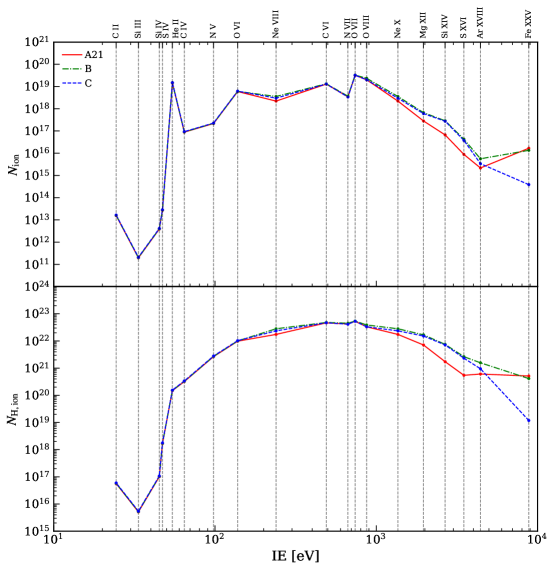
Figure 6: Column densities as functions of ionization energy. Top panel: the column density of a given ion (the ionic column density, $N_{\rm ion}$) as a function of IE of that ion (see also Table 3). Bottom panel: as above but with $N_{\rm ion}$ corrected for the element abundance ($N_{\rm ion}/A$), so it is the hydrogen column density in the region where a given ion is present.

4 Results

As one would expect based on the values of the AMD, our models are associated with significant ionic column densities for ions spanning a large range of ionization energy (IE). In Table 3, we list the results of our calculations of ionic column density for the steady models. We also plot these ionic column densities and their values corrected for the element abundance, i.e., $N_{ion}/A$, i.e. the hydrogen column density in the region where the given ion is present, in Fig. 6 (see the top and bottom panel respectively). These results show that there can be significant absorption in lines due to ions of the abundant elements, especially if they are mildly to highly ionized (e.g., He II, C VI, O VII, and O VIII). On the other hand, ions with IE less than that of He II are expected to produce weak absorption.

In §4.1, we first analyze line profiles computed for steady state solutions. Then in §4.2, we analyze those of unsteady versions of our thermally unstable models (B and C).

4.1 Steady state wind solutions

In Fig. 7, we highlight the absorption profiles for the same ions that we used to illustrate the ionization stratification in section 2 (i.e., Fe XXV, Si XIV, Mg XII, O VIII, and C IV). In Fig. 8, we show profiles for our full selection of lines for various ions, including those shown in Fig. 7. Note that in both the figures, for the doublet lines, we plot the total profile by adding the profiles due to the red and blue components. In Fig. 8, however, we also show the individual profiles due to these components using red and blue dashed lines, respectively. To aid connection between the wind solution and the line profiles, in the bottom panels of these figures, we plot $\xi$ as a function of $v$.

Line profiles in our sample belong to one of four major categories: 1) Gaussian (typical for weak lines, e.g., the S IV line), 2) boxy (lines with a strong broad core, e.g., the C IV line, 3) boxy with an extend blue wing (e.g., Mg XII), and 4) weak extended (e.g., Fe XXV). Below we will focus on the last three categories.

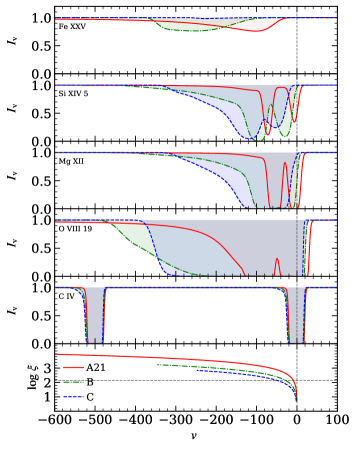
Figure 7: Absorption profiles due to lines from five ions (as labeled) together with a plot of $\xi$ vs. $v$ (bottom panel). Red solid, green dot-dashed, and blue dashed lines denote model A21, B and C, respectively. Absorption troughs are shaded to highlight their depth and shape. Except for Fe XXV, all lines shown here are doublets (see Table 2 for details). The C IV doublet components (second from the bottom panel) are separated in all three models whereas the Si XIV 5, Mg XII, and O VIII 19 doublet components are blended. The vertical grey dashed line marks $v=0$ in all panels. In the lowermost panel, the horizontal dashed line marks $\log(\xi_{\rm c,max})=2.15$ in order to judge the blueshift at which the flow enters the lower TI zone.

The troughs of the C IV, O VIII 19 and Mg XII show black saturation. The profile of the red component of the UV C IV line is relatively simple. It has a boxy shape and its width is determined by the line saturation. The line has a relatively sharp transition from the very optically thick core to the line wings. However, the profile is not exactly symmetric because even though the line forming region is near the wind base, it still has non-zero bulk velocity (see fig. 2). Therefore, the blue wing of the line is broader than the red wing due to a Doppler blueshift. The C IV profile is similar for all three wind models because the wind solutions are also similar at the base. The main difference is the line width: it increases from model A21 through B to C and this order is consistent with the order of the velocity at which $\xi=\xi_{c,max}$ (compare the bottom panel in Fig. 7 with the panel immediately above). These subtle differences are in contrast with the other profiles shown in this figure, with different models producing quite different line profiles; these are all X-ray lines with significant opacity above the the wind base.

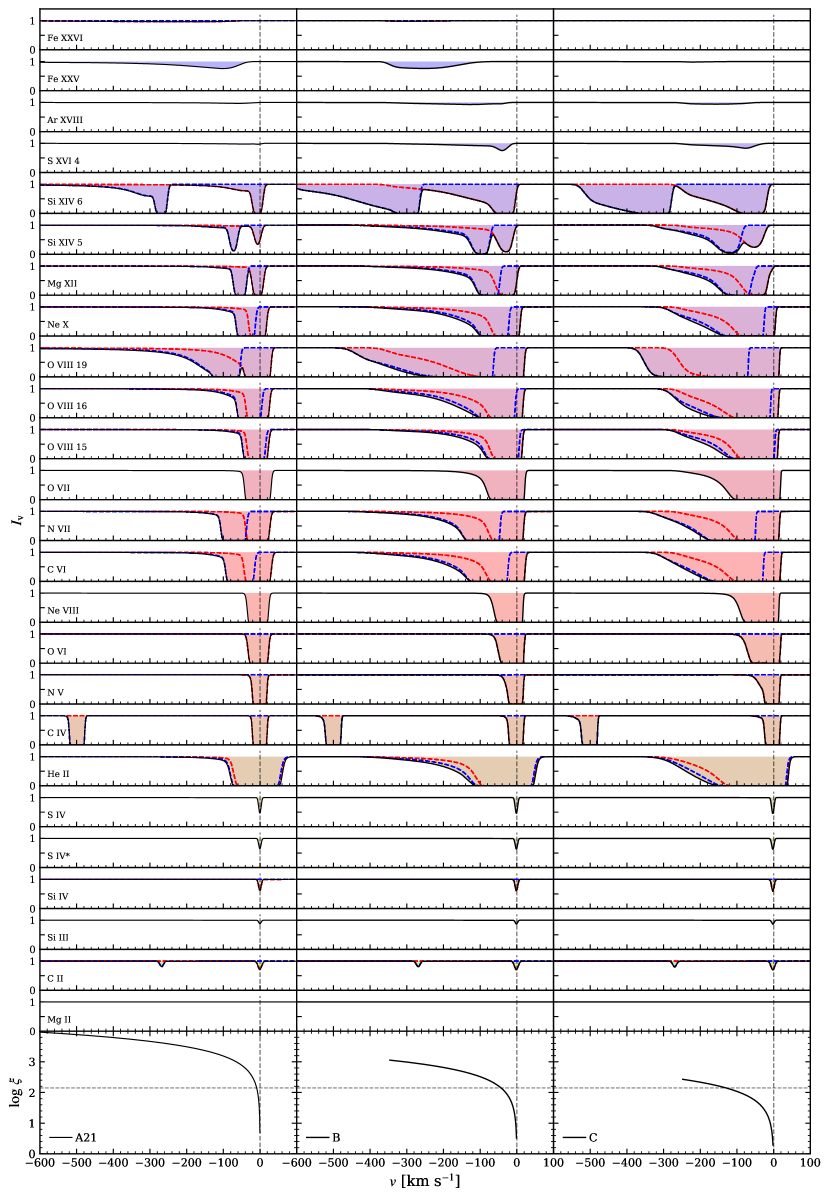
Figure 8: Absorption profiles for models A21, B and C (left, middle, and right columns of panels, respectively). See the ion labels at left and Table 2 for the line identification. The profiles are shown using solid black lines. For doublet lines, we plot a composite spectrum by adding the red and blue components while accounting for their wavelength separation in velocity space. The individual components have been additionally plotted with red and blue dashed lines. In the bottom panel, we plot the ionization parameter against the radial flow velocity, for reference. The dashed horizontal line indicates the value of $\xi_{c,max}$, whereas the black vertical line marks zero velocity.For FITS files of all our line profile calculations, see: http://www.physics.unlv.edu/astro/clumpywindsims-lps.html.

The profiles of the O VIII 19, Mg XII and Si XIV 5 lines are narrower, less blueshifted, and even weaker for model A21 than for models B and C, and this might seem contradictory to the fact that the wind in model A21 is the fastest. However, the lines probe the conditions where the population of their lower levels are the largest, and as we showed in the previous section, the $n_{1}$ distribution of their corresponding ions peaks within a relatively narrow velocity range that does not include the fast part of the wind. That is, ionization stratification may cause the signature for any individual line to be diminished and not reflect on the entire wind solution. In addition, the strong runaway heating in model A21 leads to a drop in the overall flow density that in turn reduces wind absorption, as can be seen in the AMD. Therefore, the absorption in these three lines at large velocities in model A21 is weaker than in the other two models.

The Fe XXV line stands out among the other lines in Fig. 7: its blueshifted trough does not extend to zero velocity. This feature is simply caused by lack of the Fe XXV ion at small velocities (see Figs. 3 and 4 for the distributions of the ion abundance).

A quick inspection of Fig. 8, where our full sample of line profiles are plotted in order of decreasing IE, reveals that the velocity of the red-edge of the lines increases overall with IE: it is negative for the low energy ions and can be positive for the high energy ions. In addition, the extent of the blue wing of strong lines mostly decreases with decreasing IE. These trends are more clearly evident in Fig. 9 that will be discussed below. The notable exception to the second trend is the He II line which is relatively wide. This is due to the fact that the line’s strong saturation is related to a relatively very high helium abundance leading to its ground level population being significant over a wide range of radii.

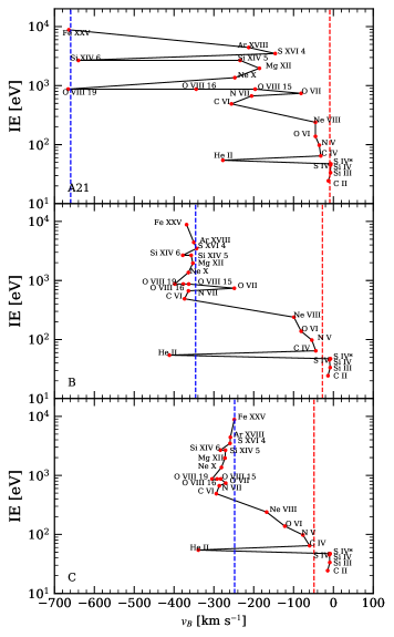
Figure 9: The position of the the blue-edge of the absorption trough, $v_{B}$ as a function of IE. We formally define $v_{B}$ as the velocity where $I_{\rm v}=0.99$. When the line is a blended doublet we correct $v_{B}$ for the doublet split. Here we show results for the steady models. The blue and red dashed lines indicate the maximum flow velocity and the velocity where ionization parameter $\log\xi=\log\xi_{c,max}=2.15$, respectively.

Fig. 8 shows that a ‘detachment’ of the line forming region from the wind base is not unique to the Fe XXV line. This is seen to a lesser degree in the profiles of the Si XIV 5 and 6 lines for model C (and lesser still for model B). Referring yet again to Fig. 4 to check if there is obvious explanation for this, we see that although models B and C have smaller terminal velocities than model A21, they are actually faster where the Si XIV ion is most abundant.

We also note that absorption in the Mg II line is absent in our models while the C II, Si III, Si IV, S IV lines are weak and symmetric. These low ionization lines form at the wind base and the maximum absorption (of the red component) is at or near zero velocity.

To quantify the extent of the blue wing, we measured the velocity at which $I_{\rm v}=0.99$ for each line. We refer to this as the blue-edge velocity, $v_{B}$, and we plot $v_{B}$ as a function of IE in Fig. 9. When the line is a blended doublet, we correct $v_{B}$ for the doublet split, while for unblended lines we measure $v_{B}$ of the red component.

Fig. 9 shows that, in general, for low IE lines, the extent of the blue wing is close to $v_{c,{\rm max}}$, the velocity at which $\xi$ approaches $\xi_{c,max}$, while $v_{B}$ is close to the maximum wind velocity for high IE lines. As mentioned above, the He II line is an exception because it is a very strongly saturated line. We note that in model A21, not all high IE lines extend to the maximum wind velocity (see e.g., Ne X and Mg XII) because the opacity of this line is relatively small at large radii for this wind solution.

The three lines of the same ion, i.e. those of O VIII, offer a good illustration of how the opacity affects the line extent. The lines of this ion have very strong and broad cores and extended blue wings. In model A21, $v_{B}$ increases with the oscillator strength, which is strongest for O VIII 19 and weakest for O VIII 15. The line absorption extends all the way to the wind maximum velocity only for the O VIII 19 line (see also Fig. 8).

Overall, the comparison of the three models shows that $v_{B}$ of high IE lines could be a good proxy for the maximum flow velocity for models B and C but for model A21, this is true only for certain high IE lines.

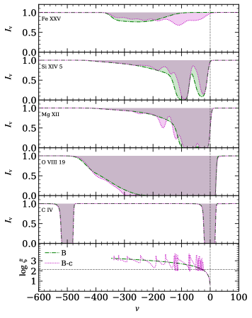
Figure 10: Line profile comparison for the steady model B (dot-dashed green shaded profile) and the unsteady/clumpy model B-c (dotted magenta shaded profile, refer to eq. 4). The lower panel shows $\log\xi$ vs $v$ for these two cases, for comparison, where horizontal gray dashed line marks $\log(\xi_{\rm c,max})=2.15$, while vertical dashed lines mark $v=0$ in all panels.

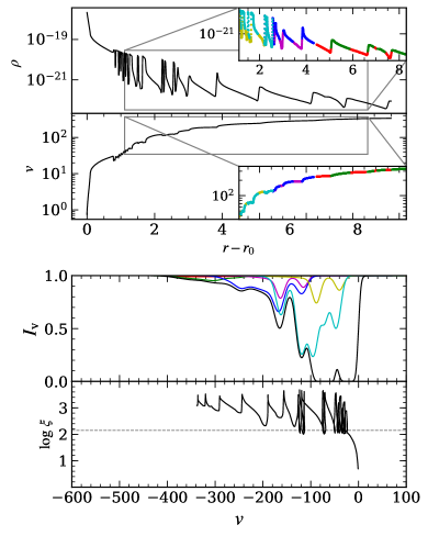
Figure 11: Contributions of different parts of a clumpy outflow (model B-c) to the overall line profile for Mg XII. The colors green, blue and cyan highlight the higher-than-average density regions corresponding to clumps, while the red, magenta and yellow highlight intercloud regions.

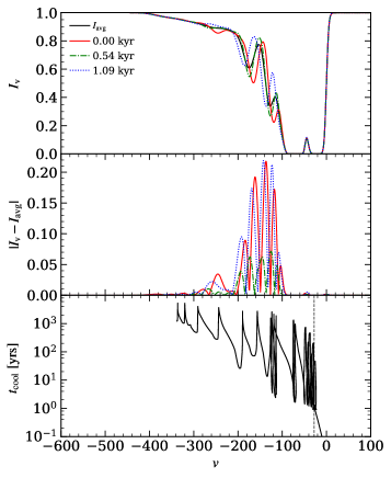
Figure 12: Variability of the Mg XII line profile for model B-c. Line profiles at three different states $t_{i}$ of the simulation runs are plotted along with the time-averaged line profile. The legend shows the time $\Delta t=(t_{i}-t_{0})$ (in kyr), the red line denoting the state $t_{0}$. The middle panel shows the difference between the snapshots from the average profile. The bottom panel shows the cooling time, $t_{\rm cool}$; a vertical line marks the velocity for which $\log\ \xi_{\rm c,max}=2.15$, showing that cooling times exceed 1 year in the clumps. Any time-dependence must therefore occur on longer timescales. An animation of the time evolution of line profiles for B-c and C-c, can be found here: http://www.physics.unlv.edu/astro/clumpywindsims-lps.html

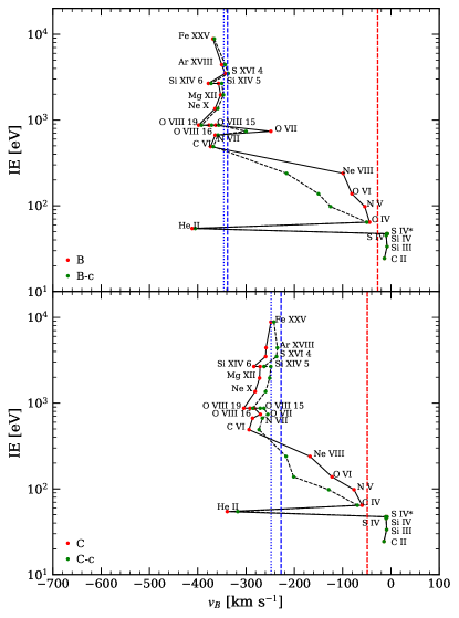
Figure 13: Ionization energy vs velocity of the blue-edge of line profiles (defined as where $I=0.99$) for steady models (black solid line with red dots) compared to their clumpy versions (black dashed line with green dots). The dotted (dashed) blue and red vertical lines indicate the maximum flow velocity and the velocity where $\xi=\xi_{\rm c,max}$, respectively, for the clumpy (steady) models.

4.2 Clumpy wind solutions

In Fig. 10, we over-plot line profiles for Model B-c (in magenta) on those for steady Model B shown previously in Fig. 7. Only one new category of line profile needs to be added to our list given in §4.1: boxy with an extended non-monotonic blue wing. It is clear from this figure that non-monotonic features can be due to either stronger or weaker absorption at different velocities and are present in all lines except those from ions with peak abundance at $\xi<\xi_{\rm c,max}$ like C IV. In other words, clumps do not affect the ‘boxy’ profiles characterizing ions formed at the wind base, as clumps are produced further downstream.

Of the remaining profiles, that of Mg XII is perhaps the most intuitive: the clumps in Model B-c can be considered over-densities superimposed on the ‘background’ wind profiles shown in Fig. 2. Hence, a deeper absorption trough should occur at the velocity where the clump resides. More distant clumps will thus have both higher velocity and lower density, so this explains the general trend that absorption troughs get less deep at higher velocities in the wing. The width of each trough is essentially $\max(\Delta v_{c},v_{\rm th})$, where $v_{\rm th}$ is the ion thermal velocity and $\Delta v_{c}$ is the range of line of sight velocities internal to the clump. As will be shown below, model C-c results in smooth line profiles because the intercloud spacing is very small. Hence, we can state that a very clumpy wind can appear completely smooth with monotonic wings if it satisfies the condition that the velocity separation of the clumps is smaller than the thermal widths. Note that similar considerations have been used to place constraints on the number of clouds in broad line regions (Arav et al., 1997).

To clearly illustrate the contribution of clumps to line profiles, Fig. 11 breaks down different density regions of the outflow in the case of the Mg XII line profile (again for model B-c). The saturated part of the absorption trough is formed at the wind base, although some of the slowest clumps do contribute. This is shown by the cyan colored regions, where absorption due to several high velocity clumps blend together to form part of the line core as well as discernible absorption troughs in the blue wing of the profile. Regions marked in green and blue are responsible for the higher velocity features that together add up to form the extended blue wing of the line. The absorption within the warm, under-dense regions between the clumps is seen to be mostly negligible (see the red, magenta and yellow colors).

In Fig. 12, we illustrate how the Mg XII line profile changes due to the evolution of the clumps in model B-c. We plot the profile at three times, $t_{i}$ (as explained in figure caption; $\Delta t=(t_{i}-t_{0})$ = {0, 0.54, 1.09} kyr). For reference, we also plot the time-averaged line profile (shown in black). The dips become increasingly blueshifted with time and also less deep as the clumps move outward with a higher velocity and become less dense. In the middle panel, we show the absolute difference between each of the three profiles and the time-averaged profile. This reveals that the largest differences occur at velocities where the line just starts to de-saturate. The bottom panel shows the cooling time,

$$t_{\rm cool}=6.6\frac{T_{5}}{n_{4}\mathcal{C}_{23}}\ \textrm{yrs}$$ (12)

where $T_{5}=T/10^{5}$ K, $n_{4}=n/10^{4}$ cm^-3 and $\mathcal{C}_{23}=\mathcal{C}/10^{23}$ is the cooling rate in units of erg cm³ s^-1. The vertical dashed line marks the velocity at which $\log\ \xi>\log\ \xi_{\rm c,max}=2.15$. Above this velocity, the cooling time is of the order of years, which indicates that the flow cannot respond to minor flux variability on timescales less than $\sim 1$ year. Note from §2.1 that we chose the time period of perturbations to be a small fraction of the dynamical time scale, but still large enough to ensure that the gas can respond.

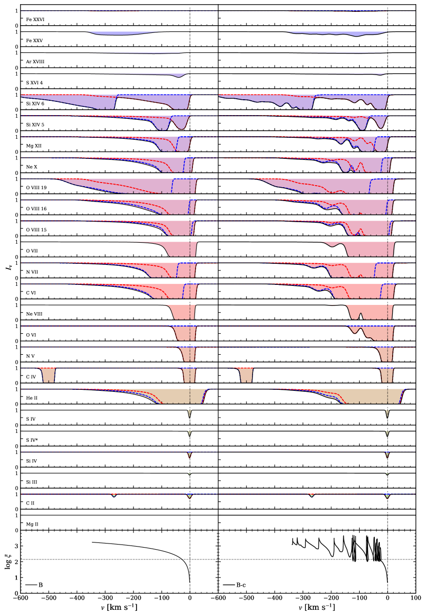
Figure 14: Same as 8, but for steady model B compared to clumpy model B-c.

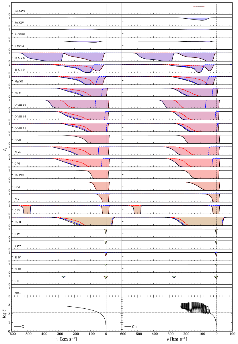
Figure 15: Same as 14, but for steady model C compared to clumpy model C-c.

In Fig. 13, we again show a plot of IE versus $v_{B}$, this time showing models B-c and C-c over-plotted with models B and C for comparison. The clumpy cases have a slightly higher overall flow velocity ($v$) (compare the blue vertical lines; dashed lines are for steady solutions and dotted lines for their clumpy counterparts). While higher IE ions show slightly lower $v_{B}$ for clumpy cases, intermediate ions show a very prominent increase in $v_{B}$ of their absorption troughs due to the presence of the clumps. This is because these ions (namely, N V, O VI, and Ne VIII) are direct probes of the temperature within the clumps and therefore deepen the absorption at the blue edge. The low IE ions, meanwhile, show no change in their $v_{B}$ values between steady and clumpy models. Again, these ions form at the base of the flow have negligible opacity within the clumps.

In Figs. 14 and 15, we compare steady and clumpy models for our entire collection of line profiles. As we mentioned above, model C-c is so clumpy that the blue wings of the line profiles remain essentially monotonic. Rather than produce distinguishable absorption troughs, small intercloud spacings simply result in an increase in the depth of line profiles for most ions. There are, however, a few cases of less deep absorption (e.g., Mg XII, O VIII, and Si XIV), and this occurs also in model B-c as seen most clearly for Si XIV 5 in Fig. 10. To explain this, note that locally, the individual clumps are isobaric, meaning the clumps are also associated with under-densities corresponding to higher temperature intercloud regions. For the ions noted, these regions have less opacity compared to smooth solutions where the temperature is intermediate between cloud and intercloud gas temperatures. Thus, the column density of ions with peak abundance in intermediate temperature gas can be less in the presence of clumps, and this accounts for the reduced absorption. Conversely, the higher column of hot gas in the presence of clumps explains the increased absorption in Fe XXV, which only forms in high temperature gas.

We conclude here that it is non-trivial to determine the wind structure based on line profiles. Despite the presence of clumps in outflows, line profiles can be smooth and monotonic under certain conditions. We also note that different velocity components are not necessarily distinctive outflows (e.g., flows launched from different geometries with different escape velocities), but are instead potentially just different parts of the same flow.

5 Discussion

The conditions for generating outflows that are heated and driven by AGN radiation place these outflows at parsec scales from the central engine, where the gas is mildly bound. Such outflows can be responsible for WAs in AGNs. In this paper, we present results from our calculations of synthetic absorption line profiles that are based on smooth/clumpy models of thermally driven outflows from AGNs. Although our calculations are based on 1D radial outflow models, we find that each model produces diverse profiles and some profiles are quite complex, especially for clumpy models. We classify our line profiles into four major categories: 1) Gaussian (typical for weak lines, e.g., the S IV line), 2) boxy (lines with a strong broad core, e.g., the C IV line, 3) boxy with an extend blue wing (e.g., Mg XII), and 4) weak extended (e.g., Fe XXV). In Figs. 8, 14, and 15, we show examples of how line widths and shapes vary depending on the ionization energy of the absorbing ion. To explore the effects of outflow clumpiness, we present the breakdown of a line profile due to Mg XII as an example (see Fig. 11). This figure shows that clumps can produce deeper absorption troughs in the blue wing compared to a smooth flow, whereas the cold slow gas at the base of the outflow dominates the line center.

One of the key outflow properties is the terminal velocity. Therefore, we check whether there are any relations between the maximum outflow velocity in our models and the predicted line properties. We found that the highly ionized ion species (such as Fe XXV) with ionization energies above 100 eV trace the fastest part of the outflows. Fig. 9 shows that line profiles due to these very highly ionized species could be strongly blueshifted. Most blueshifts from these ions are comparable to the outflow terminal velocity in our thermally unstable solutions, both steady state and clumpy versions. In our thermally stable model A21, however, the blue line wing is very extended and weak so that the blue end is difficult to determine. If one then uses the width of the strong, often saturated core of the line, the wind velocity can be underestimated by an order of magnitude.

Our outflow models produce line profiles that are unlike those expected for a spherical flow. For example, winds from OB stars can be well approximated as 1D spherical outflows and their absorption profiles show maximum absorption near the highest velocities (e.g., Lamers & Cassinelli, 1999). Our profiles show maximum absorption near zero velocity which is more characteristic of bipolar disk winds in cataclysmic variables (see e.g. Drew, 1987). We realize that in both winds from OB stars and in winds from cataclysmic variables, line emission is important. Nevertheless, this simple comparison illustrates that even smooth spherical winds can produce surprising line profiles that at least superficially show similarities to profiles produced by axisymmetric disk wind calculations, a good example being the diverse line profiles shown by Giustini & Proga (2012). However, in disk winds the diversity is typically due to the line profile dependence on the inclination angle. Here we report on the importance of the wind ionization structure (see also the ionization stratification effects on line profiles in Waters et al., 2021, which is our companion paper on clumpy thermally driven disk winds).

We note the line profiles of our clumpy solutions are characterized by significantly non-monotonic blue wings only if the separation in velocity space between individual clumps is greater than the thermal width of the gas within and between the clumps. This is the difference between our models B-c and C-c (compare Figs. 14 and 15); the non-monotonic wings in model B-c are due to clumps producing blueshifted absorption troughs at velocities outside of the line core. Additionally, the small clump spacing in a highly clumped model like C-c, results in smaller columns of intercloud gas, which are at temperatures where the opacity of certain lines (S XVI and Si XIV) reach peak values. A close comparison of the left and right panels in Figs. 15 revealed that these lines are actually weaker in model C-c compared to smooth model C.

Future X-ray observatories equipped with micro-calorimeters, such as the X-ray Imaging and Spectroscopy Mission (XRISM Science Team, 2020, launch expected in 2022) and the Advanced Telescope for High ENergy Astrophysics (Athena; Nandra et al., 2013, launch expected in the 2030s) mission should permit distinguishing different shapes of absorption line profiles and should also allow characterizing clump-like features in the X-ray spectra of nearby AGN such as NGC 5548, if present. Spectra from these observatories will provide a uniform energy resolution down to a few eV over a wide energy range, including in the Fe K band, allowing velocity features of only a few km s^-1 to be resolved. Despite the great wealth of current observational data, these future spectral resolutions are needed for the precise comparison of our models for WAs due to the relatively small velocities involved (e.g., see Laha2021, for a recent review).

Our main conclusion is that thermally driven wind solutions constitute viable models for WAs. Therefore, we plan to further develop these models, as well as to increase the fidelity of our line profile calculations. We finish the paper by mentioning just a few of the future developments we have planned.

To better treat line saturation, we plan to implement Lorentzian profiles instead of Gaussian profiles. In addition, it is of course important to consider the contribution of emission to absorption line profile calculations. Indeed, Lucy (1983) showed that non-monotonic velocity profiles in O star winds give rise to saturated P Cygni profiles with flat bottoms. For our future work, we expect that exploration of emission line profiles could result in significant emission lines near $v=0$, which could extend to larger velocities and make absorption appear weaker. Studies of X-ray binaries where AGN-like warm absorbers are sometimes observed show that the line emission could be indeed important (i.e., Miller et al., 2002, 2004).

On the hydrodynamical modeling side, we compared conduction and cooling timescales and found that thermal conduction may be important, especially in regions between clumps that have high temperature contrasts (the importance of including thermal conduction in local cloud simulations has already been demonstrated; e.g. Proga & Waters, 2015). Therefore, we plan to assess the effects of thermal conduction on line profiles in our future calculations. Finally, the time variability due to clump evolution on observable timescales is insignificant, as shown in Fig. 12. This may be indicative of the limitations of our assumption of pure photoionization models in thermal equilibrium. We therefore plan to assess if non-equilibrium effects can be important.

References

- Arav et al. (1997) Arav, N., Barlow, T. A., Laor, A., & Blandford, R. D. 1997, MNRAS, 288, 1015, doi: 10.1093/mnras/288.4.1015
- Balbus (1986) Balbus, S. A. 1986, ApJ, 303, L79, doi: 10.1086/184657
- Balsara & Krolik (1993) Balsara, D. S., & Krolik, J. H. 1993, ApJ, 402, 109, doi: 10.1086/172116
- Barai et al. (2012) Barai, P., Proga, D., & Nagamine, K. 2012, MNRAS, 424, 728, doi: 10.1111/j.1365-2966.2012.21260.x
- Begelman et al. (1983) Begelman, M. C., McKee, C. F., & Shields, G. A. 1983, ApJ, 271, 70, doi: 10.1086/161178
- Behar (2009) Behar, E. 2009, The Astrophysical Journal, 703, 1346, doi: 10.1088/0004-637x/703/2/1346
- Blondin (1994) Blondin, J. M. 1994, ApJ, 435, 756, doi: 10.1086/174853
- Blustin et al. (2005) Blustin, A. J., Page, M. J., Fuerst, S. V., Brand uardi-Raymont, G., & Ashton, C. E. 2005, A&A, 431, 111, doi: 10.1051/0004-6361:20041775
- Crenshaw et al. (1999) Crenshaw, D. M., Kraemer, S. B., Boggess, A., et al. 1999, ApJ, 516, 750, doi: 10.1086/307144
- Dannen et al. (2019) Dannen, R. C., Proga, D., Kallman, T. R., & Waters, T. 2019, ApJ, 882, 99, doi: 10.3847/1538-4357/ab340b
- Dannen et al. (2020) Dannen, R. C., Proga, D., Waters, T., & Dyda, S. 2020, ApJ, 893, L34, doi: 10.3847/2041-8213/ab87a5
- Dorodnitsyn et al. (2012) Dorodnitsyn, A., Kallman, T., & Bisnovatyi-Kogan, G. S. 2012, ApJ, 747, 8, doi: 10.1088/0004-637X/747/1/8
- Dorodnitsyn et al. (2008a) Dorodnitsyn, A., Kallman, T., & Proga, D. 2008a, ApJ, 675, L5, doi: 10.1086/529374
- Dorodnitsyn et al. (2008b) —. 2008b, ApJ, 687, 97, doi: 10.1086/591418
- Dorodnitsyn et al. (2016) —. 2016, ApJ, 819, 115, doi: 10.3847/0004-637X/819/2/115
- Drew (1987) Drew, J. E. 1987, MNRAS, 224, 595, doi: 10.1093/mnras/224.3.595
- Dyda et al. (2017) Dyda, S., Dannen, R., Waters, T., & Proga, D. 2017, MNRAS, 467, 4161, doi: 10.1093/mnras/stx406
- Ebrero et al. (2016) Ebrero, J., Kriss, G. A., Kaastra, J. S., & Ely, J. C. 2016, A&A, 586, A72, doi: 10.1051/0004-6361/201527495
- Everett & Murray (2007) Everett, J. E., & Murray, N. 2007, ApJ, 656, 93, doi: 10.1086/510324
- Field (1965) Field, G. B. 1965, ApJ, 142, 531, doi: 10.1086/148317
- Fu et al. (2017) Fu, X.-D., Zhang, S.-N., Sun, W., Niu, S., & Ji, L. 2017, Research in Astronomy and Astrophysics, 17, 095, doi: 10.1088/1674-4527/17/9/95
- Gabel et al. (2003) Gabel, J. R., Crenshaw, D. M., Kraemer, S. B., et al. 2003, ApJ, 583, 178, doi: 10.1086/345096
- Gaspari et al. (2013) Gaspari, M., Ruszkowski, M., & Oh, S. P. 2013, MNRAS, 432, 3401, doi: 10.1093/mnras/stt692
- Giustini & Proga (2012) Giustini, M., & Proga, D. 2012, ApJ, 758, 70, doi: 10.1088/0004-637X/758/1/70
- Holczer et al. (2007) Holczer, T., Behar, E., & Kaspi, S. 2007, The Astrophysical Journal, 663, 799, doi: 10.1086/518416
- Kallman & Bautista (2001) Kallman, T., & Bautista, M. 2001, ApJS, 133, 221, doi: 10.1086/319184
- Kallman & Dorodnitsyn (2019) Kallman, T., & Dorodnitsyn, A. 2019, ApJ, 884, 111, doi: 10.3847/1538-4357/ab40aa
- Kurosawa & Proga (2009a) Kurosawa, R., & Proga, D. 2009a, ApJ, 693, 1929, doi: 10.1088/0004-637X/693/2/1929
- Kurosawa & Proga (2009b) —. 2009b, MNRAS, 397, 1791, doi: 10.1111/j.1365-2966.2009.15084.x
- Laha et al. (2014) Laha, S., Guainazzi, M., Dewangan, G. C., Chakravorty, S., & Kembhavi, A. K. 2014, MNRAS, 441, 2613, doi: 10.1093/mnras/stu669
- Lamers & Cassinelli (1999) Lamers, H. J. G. L. M., & Cassinelli, J. P. 1999, Introduction to Stellar Winds (Cambridge)
- Longinotti et al. (2013) Longinotti, A. L., Krongold, Y., Kriss, G. A., et al. 2013, ApJ, 766, 104, doi: 10.1088/0004-637X/766/2/104
- Lucy (1983) Lucy, L. B. 1983, ApJ, 274, 372, doi: 10.1086/161453
- McKernan et al. (2007) McKernan, B., Yaqoob, T., & Reynolds, C. S. 2007, MNRAS, 379, 1359, doi: 10.1111/j.1365-2966.2007.11993.x
- Mehdipour et al. (2015) Mehdipour, M., Kaastra, J. S., Kriss, G. A., et al. 2015, A&A, 575, A22, doi: 10.1051/0004-6361/201425373
- Mehdipour et al. (2017) —. 2017, A&A, 607, A28, doi: 10.1051/0004-6361/201731175
- Miller et al. (2002) Miller, J. M., Fabian, A. C., Wijnands, R., et al. 2002, ApJ, 578, 348, doi: 10.1086/342466
- Miller et al. (2004) Miller, J. M., Raymond, J., Fabian, A. C., et al. 2004, ApJ, 601, 450, doi: 10.1086/380196
- Mizumoto et al. (2019) Mizumoto, M., Done, C., Tomaru, R., & Edwards, I. 2019, MNRAS, 489, 1152, doi: 10.1093/mnras/stz2225
- Mościbrodzka & Proga (2013) Mościbrodzka, M., & Proga, D. 2013, ApJ, 767, 156, doi: 10.1088/0004-637X/767/2/156
- Nandra et al. (2013) Nandra, K., Barret, D., Barcons, X., et al. 2013, arXiv e-prints, arXiv:1306.2307. https://arxiv.org/abs/1306.2307
- Proga (2007) Proga, D. 2007, ApJ, 661, 693, doi: 10.1086/515389
- Proga et al. (2008) Proga, D., Ostriker, J. P., & Kurosawa, R. 2008, ApJ, 676, 101, doi: 10.1086/527535
- Proga & Waters (2015) Proga, D., & Waters, T. 2015, ApJ, 804, 137, doi: 10.1088/0004-637X/804/2/137
- Reynolds (1997) Reynolds, C. S. 1997, MNRAS, 286, 513, doi: 10.1093/mnras/286.3.513
- Ricci et al. (2017) Ricci, C., Trakhtenbrot, B., Koss, M. J., et al. 2017, Nature, 549, 488, doi: 10.1038/nature23906
- Shields & Hamann (1997) Shields, J. C., & Hamann, F. 1997, ApJ, 481, 752, doi: 10.1086/304070
- Sim et al. (2012) Sim, S. A., Proga, D., Kurosawa, R., et al. 2012, MNRAS, 426, 2859, doi: 10.1111/j.1365-2966.2012.21816.x
- Stone et al. (2020) Stone, J. M., Tomida, K., White, C. J., & Felker, K. G. 2020, arXiv e-prints, arXiv:2005.06651. https://arxiv.org/abs/2005.06651
- Takeuchi et al. (2013) Takeuchi, S., Ohsuga, K., & Mineshige, S. 2013, PASJ, 65, 88, doi: 10.1093/pasj/65.4.88
- Waters et al. (2021) Waters, T., Proga, D., & Dannen, R. 2021, arXiv e-prints, arXiv:2101.09273. https://arxiv.org/abs/2101.09273
- Waters et al. (2017) Waters, T., Proga, D., Dannen, R., & Kallman, T. R. 2017, MNRAS, 467, 3160, doi: 10.1093/mnras/stx238
- Woods et al. (1996) Woods, D. T., Klein, R. I., Castor, J. I., McKee, C. F., & Bell, J. B. 1996, ApJ, 461, 767, doi: 10.1086/177101
- XRISM Science Team (2020) XRISM Science Team. 2020, arXiv e-prints, arXiv:2003.04962. https://arxiv.org/abs/2003.04962