Nesterov Acceleration for Equality-Constrained Convex Optimization via Continuously Differentiable Penalty Functions

Abstract

We propose a framework to use Nesterov’s accelerated method for constrained convex optimization problems. Our approach consists of first reformulating the original problem as an unconstrained optimization problem using a continuously differentiable exact penalty function. This reformulation is based on replacing the Lagrange multipliers in the augmented Lagrangian of the original problem by Lagrange multiplier functions. The expressions of these Lagrange multiplier functions, which depend upon the gradients of the objective function and the constraints, can make the unconstrained penalty function non-convex in general even if the original problem is convex. We establish sufficient conditions on the objective function and the constraints of the original problem under which the unconstrained penalty function is convex. This enables us to use Nesterov’s accelerated gradient method for unconstrained convex optimization and achieve a guaranteed rate of convergence which is better than the state-of-the-art first-order algorithms for constrained convex optimization. Simulations illustrate our results.

I Introduction

Convex optimization problems arise in areas like signal processing, control systems, estimation, communication, data analysis, and machine learning. They are also useful to bound the optimal values of certain nonlinear programming problems, and to approximate their optimizers. Due to their ubiquitous nature and importance, much effort has been devoted to efficiently solve them. This paper is motivated by the goal of designing fast methods that combine the simplicity and ease of gradient methods with acceleration techniques to efficiently solve constrained optimization problems.

Literature review: Gradient descent is a widespread method to solve unconstrained convex optimization problems. However, gradient descent suffers from slow convergence. To achieve local quadratic convergence, one can use Newton’s method [1]. Newton’s method uses second-order information of the objective function and requires the inversion of the Hessian of the function. In contrast, the accelerated gradient descent method proposed by Nesterov [2] uses only first-order information combined with momentum terms [3, 4] to achieve an optimal convergence rate. For constrained convex optimization, generalizations of gradient algorithms include the projected gradient descent [5] (for simple set constraints where the projection of any point can be computed in closed form) and (continuous-time) saddle-point or primal-dual dynamics (for general constraints), see e.g., [6, 7, 8, 9]. When the saddle function is strongly convex-strongly concave, the primal-dual dynamics converges exponentially fast, see e.g., [10]. Recent work [11, 12, 13, 14] has explored the partial relaxation of the strong convexity requirement while retaining the exponential convergence rate. A method with improved rate of convergence for constrained problems is accelerated mirror descent [15] which, however necessitates the choice of an appropriate mirror map depending on the geometry of the problem and requires that each update solves a constrained optimization problem (which might be challenging itself). Some works [16, 17, 18] have sought to generalize Newton’s method for equality constrained problems, designing second-order updates that require the inversion of the Hessian matrix of the augmented Lagrangian. Similar to gradient descent, a generalization of Nesterov’s method for constrained convex optimization described in [5] uses the projection for simple set constraints. Here we follow an alternative route involving continuously differentiable exact penalty functions [19, 20] to convert the original problem into the unconstrained optimization of a nonlinear function. The works [21, 22, 23] generalize these penalty functions and establish, under appropriate assumptions on the constraint set, complete equivalence between the solutions of the constrained and unconstrained problems. We employ these penalty functions to reformulate the constrained convex optimization problem and identify sufficient conditions under which the unconstrained problem is also convex. Our previous work [24] explores the distributed computation of the gradient of the penalty function when the objective is separable and the constraints are locally expressible.

Statement of contributions: We consider equality-constrained convex optimization problems. Our starting point is the exact reformulation of this problem as the optimization of an unconstrained continuously differentiable function. We show via a counterexample that the unconstrained penalty function might not be convex for any value of the penalty parameter even if the original problem is convex. This motivates our study of sufficient conditions on the objective and constraint functions of the original problem for the unconstrained penalty function to be convex. Our results are based on analyzing the positive semi-definiteness of the Hessian of the penalty function. We provide explicit bounds below which, for any value of the penalty parameter, the penalty function is either convex or strongly convex on the domain, resp. Since the optimizers of the unconstrained convex penalty function are the same as the optimizers of the original problem, we deduce that the proposed Nesterov implementation solves the original constrained problem with an accelerated convergence rate starting from an arbitrary initial condition. Finally, we establish that Nesterov’s algorithm applied to the penalty function renders the feasible set forward invariant. This, coupled with the fact that the penalty terms vanish on the feasible set, ensures that the accelerated convergence rate is also achieved from any feasible initialization.

II Preliminaries

We collect here basic notions of convex analysis [25, 1] and optimization [26].

Convex Analysis: Let $\operatorname{\mathcal{C}}\subseteq^{n}$ be a convex set. A function $f:^{n}\rightarrow$ is convex on $\operatorname{\mathcal{C}}$ if $f(\lambda x+(1-\lambda)y)\leq\lambda f(x)+(1-\lambda)f(y)$, for all $x,y\in\operatorname{\mathcal{C}}$ and $\lambda\in[0,1]$. Convex functions have the property of having the same local and global minimizers. A continuously differentiable $f:^{n}\rightarrow$ is convex on $\operatorname{\mathcal{C}}$ iff $f(y)\geq f(x)+(y-x)^{\top}\nabla f(x)$, for all $x,y\in\operatorname{\mathcal{C}}$. A twice differentiable function is convex iff its Hessian is positive semi-definite. A twice differentiable function $f:^{n}\rightarrow$ is strongly convex on $\operatorname{\mathcal{C}}$ with parameter $c\in\mathbb{R}_{>0}$ iff $\nabla^{2}f(x)\geq cI$ for all $x\in\operatorname{\mathcal{C}}$.

Constrained Optimization: Consider the following nonlinear optimization problem

$$\min_{x\in\mathcal{D}} f(x)$$ (1)

  s.t. $$h(x)=0,$$

where $f:^{n}\rightarrow,\;h:^{n}\rightarrow^{p}$ are twice continuously differentiable functions with $p\leq n$ and $\mathcal{D}\subset^{n}$ is a compact set which is regular (i.e., $\operatorname{\mathcal{D}}=\overline{\mathcal{D}^{o}}$). The feasible set of (1) is $\operatorname{\mathcal{F}}=\{x\in\mathcal{D}\;|\;h(x)=0\}$. Linear independence constraint qualification (LICQ) holds at $x\in^{n}$ if $\{\nabla h_{k}(x)\}_{k\in\{1,\dots,p\}}$ are linearly independent.

The Lagrangian $L:^{n}\times^{p}\rightarrow$ associated to (1) is

$$L(x,\mu)=f(x)+\mu^{\top}h(x),$$

where $\mu\in^{p}$ is the Lagrange multiplier (also called dual variable) associated with the constraints. A Karush-Kuhn-Tucker (KKT) point for (1) is $(\bar{x},\bar{\mu})$ such that

$$\nabla_{x}L(\bar{x},\bar{\mu}) =0,\qquad\quad h(\bar{x})=0.$$

Under LICQ, the KKT conditions are necessary for a point to be locally optimal.

Continuously Differentiable Exact Penalty Functions: With exact penalty functions, the idea is to replace the constrained optimization problem (1) by an equivalent unconstrained problem. Here, we discuss continuously differentiable exact penalty functions following [20, 21]. The key observation is that one can interpret a KKT tuple as establishing a relationship between a primal optimal solution $\bar{x}$ and the dual optimal $\bar{\mu}$. In turn, the following result introduces multiplier functions that extend this relationship to any $x\in^{n}$.

Proposition II.1.

(Multiplier functions and their derivatives [21]): Assume that LICQ is satisfied at all $x\in\mathcal{D}$. Define $N:^{n}\rightarrow^{p\times p}$ as $N(x)=\nabla h(x)^{\top}\nabla h(x)$. Then $N(x)$ is a positive definite matrix for all $x\in\operatorname{\mathcal{D}}$. Given the function $x\mapsto\mu(x)$ defined by $\mu(x)=-N^{-1}(x)\nabla h(x)^{\top}\nabla f(x)$, the following holds

1. if $(\bar{x},\bar{\mu})$ is a KKT point for (1), then $\mu(\bar{x})=\bar{\mu}$;

2. $\mu:^{n}\rightarrow^{p}$ is a continuously differentiable function.

The multiplier function can be used to replace the multiplier vector in the augmented Lagrangian to define a continuously differentiable exact penalty function. Consider the continuously differentiable function $f^{\epsilon}:^{n}\rightarrow$,

$$f^{\epsilon}(x) =f(x)+\mu(x)^{\top}h(x)+\frac{1}{\epsilon}\|h(x)\|^{2}.$$ (2)

The next result shows when $f^{\epsilon}$ is an exact penalty function.

Proposition II.2.

(Continuously differentiable exact penalty function [21]): Assume LICQ is satisfied at all $x\in\mathcal{D}$ and consider the unconstrained problem

$$\min_{x\in\mathcal{D}^{o}}f^{\epsilon}(x).$$ (3)

Then, there exists $\bar{\epsilon}$ such that the set of global minimizers of (1) and (3) are equal for all $\epsilon\in(0,\bar{\epsilon}]$.

III Problem Statement

Consider the following convex optimization problem

$$\min_{x\in\mathcal{D}} f(x)$$ (4)

  s.t. $$Ax-b=0,$$

where $f:^{n}\rightarrow$ is a twice continuously differentiable convex function and $\mathcal{D}$ is a convex set. Here $A\in^{p\times n}$ and $b\in^{p}$ with $p<n$. Without loss of generality, we assume $A$ has full row rank (implying that LICQ holds at all $x\in^{n}$).

Our aim is to design a Nesterov-like fast method to solve (4). We do this by reformulating the problem as an unconstrained optimization using continuously differentiable penalty function methods, cf. Section II. Then, we employ the Nesterov’s accelerated gradient method to design

$$x_{k+1} =y_{k}-\alpha\nabla f^{\epsilon}(y_{k}),$$ (5a)

$$a_{k+1} =\frac{1+\sqrt{4a_{k}^{2}+1}}{2},$$ (5b)

$$y_{k+1} =x_{k+1}+\frac{a_{k}-1}{a_{k+1}}(x_{k+1}-x_{k}),$$ (5c)

where $\alpha\in\mathbb{R}_{>0}$ is the stepsize. If $f^{\epsilon}$ is convex with Lipschitz gradient $L$ and the algorithm is initialized at an arbitrary initial condition $x_{0}$ with $y_{0}=x_{0}$ and $a_{0}=1$, then according to [2, Theorem 1],

$$f^{\epsilon}(x_{k})-f^{\epsilon}(x^{*})\leq\dfrac{C}{(k+1)^{2}},$$ (6a)

where $$x^{*}\in^{n} f^{\epsilon} C\in\mathbb{R}_{\geq 0} L f^{\epsilon} s\in\mathbb{R}_{>0}$$ is a global minimizer of and is a constant dependant upon the initial condition and . If is strongly convex with parameter , and (5b) and (5c) are replaced by

$$y_{k+1} =x_{k+1}+\frac{\sqrt{L}-\sqrt{s}}{\sqrt{L}+\sqrt{s}}(x_{k+1}-x_{k}),$$ (5d)

then one has from [5, Theorem 2.2.1]

$$f^{\epsilon}(x_{k})-f^{\epsilon}(x^{*})\leq C_{s}\exp\left(-k\sqrt{\frac{s}{L}}\right),$$ (6b)

where $C_{s}\in\mathbb{R}_{\geq 0}$ is a constant dependant upon the initial condition, $s$, and $L$. The key technical point for this approach to be successful is to ensure that the penalty function $f^{\epsilon}$ is (strongly) convex. Section IV below shows that this is indeed the case for suitable values of the penalty parameter under appropriate assumptions on the objective and constraint functions of the original problem (4).

Remark 1.

(Distributed Algorithm Implementation): We note here that the algorithm (5) is amenable to distributed implementation if the objective function is separable and the constraints are locally coupled. In fact, our previous work [24] has shown how, in this case, the computation of the gradient of the penalty function in (5a) can be implemented in a distributed way. Based on this observation, one could use the framework proposed here for fast optimization of convex problems in a distributed way. To obtain fast convergence, one could also use second-order augmented Lagrangian methods, e.g., [17, 18], but their distributed implementation faces the challenge of computing the inverse of the Hessian of the augmented Lagrangian to update the primal and dual variables. Even if the Hessian is sparse for separable objective functions and local constraints, its inverse in general is not. $\bullet$

IV Convexity of the Penalty Function

We start by showing that the continuously differentiable exact penalty function $f^{\epsilon}$ defined in (2) might not be convex even if the original problem (4) is convex. For the convex problem (4), the penalty function takes the form

$$f^{\epsilon}(x) =f(x)$$ (7)

$$\quad-([AA^{\top}]^{-1}A\nabla f(x))^{\top}(Ax-b)+\frac{1}{\epsilon}\|Ax-b\|^{2}.$$

A look at this expression makes it seem like a sufficiently small choice of $\epsilon$ might make $f^{\epsilon}$ convex for all $x\in\mathcal{D}$. The following shows that this is always not the case.

Example 1.

(Non-convex penalty function): Consider

$$\min\limits_{x\in\mathcal{D}} x_{1}^{4}+x_{2}^{4}$$

  s.t. $$x_{1}+x_{2}=0.$$

The optimizer is $(0,0)$. The penalty function takes the form

$$f^{\epsilon}(x)=x_{1}^{4}+x_{2}^{4}+\mu(x)^{\top}(x_{1}+x_{2})+\dfrac{1}{\epsilon}(x_{1}+x_{2})^{2},$$

where $\mu(x)=-(2x_{1}^{3}+2x_{2}^{3})$. The Hessian of this function is

$$\nabla^{2}f^{\epsilon}(x)\!=\!\!\left[\begin{matrix}-12x_{1}^{2}-12x_{1}x_{2}+\dfrac{2}{\epsilon}&-6x_{1}^{2}-6x_{2}^{2}+\dfrac{2}{\epsilon}\\ -6x_{1}^{2}-6x_{2}^{2}+\dfrac{2}{\epsilon}&-12x_{2}^{2}-12x_{1}x_{2}+\dfrac{2}{\epsilon}\end{matrix}\right]\!.$$

If $x_{1}=0$, then the determinant of $\nabla^{2}f^{\epsilon}(x)$ evaluates to $-36x_{2}^{4}$, which is independent of $\epsilon$. Hence, $f^{\epsilon}$ cannot be made convex over any set containing the vertical axis. $\bullet$

Example 1 shows that the penalty function cannot always be convexified by adjusting the value of $\epsilon$. Intuitively, the reason for this fact is that the term susceptible to be scaled in the expression (7) which depends on the parameter $\epsilon$ is not strongly convex. This implies that there are certain subspaces where non-convexity arising from the term that involve the Lagrange multiplier function cannot be countered. In turn, these subspaces are defined by the kernel of the Hessian of the last term in the expression (7) of the penalty function.

These observations motivate our study of conditions on the objective function and the constraints that guarantee that the penalty function is convex. In our discussion, we start by providing sufficient conditions for the convexity of the penalty function over $\operatorname{\mathcal{D}}$.

IV-A Sufficient Conditions for Convexity over the Domain

Here we provide conditions for the convexity of the penalty function $f^{\epsilon}$ by establishing the positive semi definiteness of its Hessian. Throughout the section, we assume $f$ is three times differentiable. Note that the gradient and the Hessian of $f^{\epsilon}$ are given, resp., by

$$\nabla f^{\epsilon}(x) =\nabla f(x)-\nabla^{2}f(x)A^{\top}[AA^{\top}]^{-1}(Ax-b)$$

$$\quad-A^{\top}[AA^{\top}]^{-1}A\nabla f(x)+\frac{2}{\epsilon}A^{\top}(Ax-b).$$ (8a)

$$\nabla^{2}f^{\epsilon}(x) =\nabla^{2}f(x)-W(x)-\nabla^{2}f(x)A^{\top}[AA^{\top}]^{-1}A$$

$$\quad-A^{\top}[AA^{\top}]^{-1}A\nabla^{2}f(x)+\frac{2}{\epsilon}A^{\top}A,$$ (8b)

where we use the short-hand notation

$$W(x)=\sum\limits_{i=1}^{n}\nabla_{x_{i}}\nabla^{2}f(x)A^{\top}[AA^{\top}]^{-1}(Ax-b)e_{i}^{n^{\top}}.$$ (9)

The following result provides sufficient conditions under which the penalty function (7) is convex on $\operatorname{\mathcal{D}}$.

Theorem IV.1.

(Convexity of the penalty function): For the optimization problem (4), assume $\nabla^{2}f(x)-W(x)\succ 0$ for all $x\in\operatorname{\mathcal{D}}$ and let

$$\bar{\epsilon}=\min\limits_{x\in\operatorname{\mathcal{D}}}\dfrac{2\lambda_{\min}(AA^{\top})\lambda_{\min}(\nabla^{2}f(x)-W(x))}{\lambda^{2}_{\max}(\nabla^{2}f(x))+R(x)\lambda_{\min}(\nabla^{2}f(x)-W(x))},$$

where $R(x)=2\lambda_{\max}(\nabla^{2}f(x))-\lambda_{\min}(\nabla^{2}f(x)-W(x))$. Then $f^{\epsilon}$ is convex on $\operatorname{\mathcal{D}}$ for all $\epsilon\in(0,\bar{\epsilon}]$ and consequently the convergence guarantee (6a) holds.

Proof:

For an arbitrary $x\in\operatorname{\mathcal{D}}$, we are interested in determining the conditions under which $\nabla^{2}f^{\epsilon}(x)\succeq 0$, or in other words, $v^{\top}\nabla^{2}f^{\epsilon}(x)v\geq 0$ for all $v\in^{n}$. From (8b),

$$v^{\top}\nabla^{2}f^{\epsilon}(x)v =\frac{2}{\epsilon}v^{\top}A^{\top}Av+v^{\top}(\nabla^{2}f(x)-W(x))v$$ (10)

$$\quad-2v^{\top}(\nabla^{2}f(x)A^{\top}[AA^{\top}]^{-1}A)v.$$

Let us decompose $v$ as $v=v^{\|}+v^{\perp}$, where $v^{\|}$ is the component of $v$ in the nullspace $\operatorname{\mathcal{N}}(A)$ of $A$ and $v^{\perp}$ is the component orthogonal to it. Then (10) becomes

$$v^{\top}\nabla^{2}f^{\epsilon}(x)v =\frac{2}{\epsilon}v^{\perp\top}A^{\top}Av^{\perp}+v^{\top}(\nabla^{2}f(x)-W(x))v$$

$$\quad-2v^{\|\top}\nabla^{2}f(x)A^{\top}[AA^{\top}]^{-1}Av^{\perp}$$

$$\quad-2v^{\perp\top}\nabla^{2}f(x)A^{\top}[AA^{\top}]^{-1}Av^{\perp}.$$

Since $A^{\top}(AA^{\top})^{-1}Av^{\perp}=v^{\perp}$, cf. [27, Theorem 1.1.1], the above expression reduces to

$$v^{\top}\nabla^{2}f^{\epsilon}(x)v=\frac{2}{\epsilon}v^{\perp\top}A^{\top}Av^{\perp}+v^{\top}(\nabla^{2}f(x)-W(x))v$$

$$\quad-2v^{\|\top}\nabla^{2}f(x)v^{\perp}-2v^{\perp\top}\nabla^{2}f(x)v^{\perp}$$

$$\geq\Big{(}\frac{2}{\epsilon}\lambda_{2}(A^{\top}A)-2\lambda_{\max}(\nabla^{2}f(x))\Big{)}\|v^{\perp}\|^{2}$$

$$\quad+\lambda_{\min}(\nabla^{2}f(x)-W(x))(\|v^{\perp}\|^{2}+\|v^{\|}\|^{2})$$

$$\quad-2\lambda_{\max}(\nabla^{2}f(x))\|v^{\perp}\|\|v^{\|}\|$$

$$=\begin{bmatrix}\!\|v^{\perp}\|\!\\ \!\|v^{\|}\|\!\end{bmatrix}^{\top}\underbrace{\begin{bmatrix}S(x)&-\lambda_{\max}(\nabla^{2}f(x))\\ \!-\lambda_{\max}(\nabla^{2}f(x))&\lambda_{\min}(\nabla^{2}f(x)-W(x))\!\end{bmatrix}}_{P(x)}\begin{bmatrix}\!\|v^{\perp}\|\!\\ \!\|v^{\|}\|\!\end{bmatrix}\!\!,$$

where $S(x)=\dfrac{2}{\epsilon}\lambda_{\min}(AA^{\top})-R(x)$. Therefore, we deduce that $\nabla^{2}f^{\epsilon}(x)\succeq 0$ if $\epsilon$ is such that $P(x)\succeq 0$. Being a $2\times 2$-matrix, the latter holds if $S(x)$ and determinant of $P(x)$ are non-negative. The determinant is non-negative if and only if

$$\epsilon\leq\dfrac{2\lambda_{\min}(AA^{\top})\lambda_{\min}(\nabla^{2}f(x)-W(x))}{\lambda^{2}_{\max}(\nabla^{2}f(x))+R(x)\lambda_{\min}(\nabla^{2}f(x)-W(x))}.$$

The above value of $\epsilon$ also ensures that $S(x)>0$. Taking the minimum over all $x\in\operatorname{\mathcal{D}}$ completes the proof. ∎

Remark 2.

(Differentiability of the objective function): Note that the implementation of (5) requires the objective function $f$ to be twice continuously differentiable, while the definition of $W$ in (9) involves the third-order partial derivatives of $f$. We believe that an extension of Theorem IV.1 could be pursued in case the objective function is only twice differentiable using tools from nonsmooth analysis, e.g., [28], but we do not pursue it here for space reasons. $\bullet$

The next result provides sufficient conditions under which the penalty function is strongly convex on $\operatorname{\mathcal{D}}$.

Corollary IV.2.

(Strong convexity of the penalty function): For the optimization problem (4), assume $\nabla^{2}f(x)-W(x)\succeq cI$ for all $x\in\operatorname{\mathcal{D}}$ and let

$$\bar{\epsilon}_{s}=\min\limits_{x\in\operatorname{\mathcal{D}}}\!\dfrac{2\lambda_{\min}(AA^{\top})(c-s)}{\lambda^{2}_{\max}(\nabla^{2}f(x))\!+\!2(c-s)\lambda_{\max}(\nabla^{2}f(x))\!-\!(c-s)^{2}\!}.$$

Then $f^{\epsilon}$ is strongly convex on $\operatorname{\mathcal{D}}$ with parameter $s\in(0,c)$ for all $\epsilon\in(0,\bar{\epsilon}_{s}]$ and the convergence guarantee (6b) holds.

Proof:

Let us decompose $\nabla^{2}f(x)-W(x)$ as $\nabla^{2}f(x)-W(x)=B(x)+sI$. Since $\nabla^{2}f(x)-W(x)\succeq cI$, it follows that $B(x)\succeq(c-s)I$. Establishing that the penalty function is strongly convex with parameter $s$ is equivalent to establishing that, for all $x\in\operatorname{\mathcal{D}}$, $v^{\top}(\nabla^{2}f^{\epsilon}(x)-sI)v\geq 0$ for all $v\in^{n}$. Following the same steps as in the proof of Theorem IV.1, one can verify that this is true if, for all $x\in\operatorname{\mathcal{D}}$, $\epsilon$ is less than or equal to

$$\dfrac{2\lambda_{\min}(AA^{\top})\lambda_{\min}(B(x))}{\lambda^{2}_{\max}(\nabla^{2}f(x))\!+\!2\lambda_{\min}(B(x))\lambda_{\max}(\nabla^{2}f(x))\!-\!\lambda^{2}_{\min}(B(x))}.$$

Replacing $\lambda_{\min}(B(x))$ by $c-s$, it follows that the penalty function is strongly convex with parameter $s$ if $\epsilon\leq\bar{\epsilon}_{s}$. ∎

It is easy to verify that Example 1 does not satisfy the sufficient condition identified in Theorem IV.1. This condition can be interpreted as requiring the original objective function to be sufficiently convex to handle the non-convexity arising from the penalty for being infeasible. Finding the value of $\bar{\epsilon}$ still remains a difficult problem as computing $\lambda_{\min}(\nabla^{2}f(x)-W(x))$ for all $x\in\operatorname{\mathcal{D}}$ is not straightforward. The next result simplifies the conditions of Theorem IV.1 for linear and quadratic programming problems.

Corollary IV.3.

(Sufficient conditions for problems with linear and quadratic objective functions):

1. If the objective function in problem (4) is linear, then the penalty function is convex on ⁿ for all values of $\epsilon$;

2. If the objective function in problem (4) is quadratic with Hessian $Q\succ 0$, then the penalty function is convex on ⁿ for all $\epsilon\in(0,\bar{\epsilon}]$, where

   $$\bar{\epsilon}=\dfrac{2\lambda_{\min}(AA^{\top})\lambda_{\min}(Q)}{\lambda^{2}_{\max}(Q)+2\lambda_{\min}(Q)\lambda_{\max}(Q)-\lambda^{2}_{\min}(Q)}.$$

In either case, the convergence guarantee (6a) holds.

Proof:

We present our arguments for each case separately. For case (i), we have $\nabla^{2}f(x)=0$. Hence,

$$\nabla^{2}f^{\epsilon}(x)=\dfrac{2}{\epsilon}A^{\top}A,$$

which means that $\nabla^{2}f^{\epsilon}(x)\geq 0$ for all $x\in^{n}$. For case (ii),

$$f(x)=\dfrac{1}{2}x^{\top}Qx+h^{\top}x,$$

where $Q\in^{n\times n}$ and $h\in^{n}$. The expression for the Hessian of $f^{\epsilon}$ becomes

$$\nabla^{2}f^{\epsilon}(x) =Q+\frac{2}{\epsilon}A^{\top}A-QA^{\top}[AA^{\top}]^{-1}A$$

$$\quad-A^{\top}[AA^{\top}]^{-1}AQ.$$

Clearly $W(x)=0$ for all $x\in^{n}$, and the result follows from Theorem IV.1. ∎

Following Corollary IV.2, one can also state similar conditions for the penalty function to be strongly convex in the case of quadratic programs, but we omit them here for space reasons. From Corollary IV.3, ensuring that the penalty function convex is easier when the objective function is quadratic. This follows from the fact that $W(x)$, which depends on the third order derivatives of the objection function, vanishes. Hence, in the quadratic case, the condition in Theorem IV.1 requiring the Hessian of the objective function to be greater than $W(x)$ for all $x\in\operatorname{\mathcal{D}}$ is automatically satisfied. In what follows we provide a very simple approach for general objective functions.

IV-B Convexity over Feasible Set Coupled with Invariance

Here we present a simplified version of the proposed approach, which is based on the fact that inside the feasible set the values of the penalty and the objective functions is the same. To build on this observation, we start by characterizing the extent to which the constraints are satisfied under the Nesterov’s algorithm.

Lemma IV.4.

(Forward invariance of the feasible set under Nesterov’s algorithm applied to the penalty function): Consider the Nesterov’s accelerated gradient algorithm (5) applied to the penalty function (7) for an arbitrary $\epsilon\geq 0$. If the algorithm is initialized at $y_{0}=x_{0}$, with $x_{0}$ belonging to the feasible set $\operatorname{\mathcal{F}}$, then $\{x_{k}\}_{k=0}^{\infty}$, $\{y_{k}\}_{k=0}^{\infty}\in\operatorname{\mathcal{F}}$.

Proof:

We need to prove that $Ax_{k}=b$ and $Ay_{k}=b$ for all $k\geq 0$ if $Ax_{0}=Ay_{0}=b$. We use the technique of mathematical induction to prove this. Since this clearly holds for $k=0$, we next prove that if $Ax_{k}=Ay_{k}=b$, then $Ax_{k+1}=Ay_{k+1}=b$. From (5a) and (8a), we have

$$Ax_{k+1}= Ay_{k}-\alpha A\nabla f^{\epsilon}(y_{k})$$

$$= Ay_{k}\!-\!\alpha A(\nabla f(y_{k})\!-\!\nabla^{2}f(y_{k})A^{\top}[AA^{\top}]^{-1}(Ay_{k}\!-\!b)$$

$$-\!A^{\top}[AA^{\top}]^{-1}A\nabla f(y_{k})\!+\!\frac{2}{\epsilon}A^{\top}(Ay_{k}\!-\!b)).$$

Substituting $Ay_{k}=b$, the above expression evaluates to $b$ independent of $\epsilon\geq 0$. Then from (5c), one has $Ay_{k+1}=b$. Since the argument above is independent of the values of $a_{k}$ for all $k\in\mathbb{N}$, it holds for the strongly convex case (5d) as well, thus completing the proof by induction. ∎

As a consequence of this result, if the trajectory starts in the feasible set $\operatorname{\mathcal{F}}$, then it remains in it forever. This observation allows us to ensure the convergence rate guarantee for any convex objective function.

Corollary IV.5.

(Accelerated convergence with feasible initialization): For the optimization problem (4) and arbitrary $\epsilon\geq 0$, the algorithm (5) initialized in $\operatorname{\mathcal{F}}$ enjoys the guarantee (6) on convergence to the optimal value.

Proof:

Note that $f^{\epsilon}(x)=f(x)$ whenever $Ax=b$, and hence by definition, is automatically (strongly) convex on $\operatorname{\mathcal{F}}$ regardless of the value of $\epsilon$. The convergence guarantee follows from this fact together with Lemma IV.4. ∎

Remark 3.

(Robustness of the proposed approach): Given any $x_{0}\in^{n}$, one can find a feasible initial point $x_{0}-A^{\top}[AA^{\top}]^{-1}(Ax_{0}-b)$ by projecting $x_{0}$ onto the feasible set $\operatorname{\mathcal{F}}$, and then implement Nesterov’s accelerated method with the projected gradient as $(I-A^{\top}[AA^{\top}]^{-1}A)\nabla f(x)$. In fact, this projected gradient method coincides with the approach proposed here when evaluated over $\operatorname{\mathcal{F}}$. The advantage of our approach resides in the incorporation of error-correcting terms incorporating the value of $Ax-b$, cf. (8a), that penalize any deviation from the feasible set and hence provide additional robustness in the face of disturbances. By contrast, the projected gradient approach requires either an error-free execution or else, if error is present, the trajectory may leave and remain outside the feasible set unless repeated projections of the updated state are taken. The inherent robustness property of the approach proposed here is especially important in the context of distributed implementations, cf. Remark 1, where agents need to collectively estimate (and hence only implement approximations of) $A^{\top}[AA^{\top}]^{-1}A\nabla f(x)$ and taking the projection in a centralized fashion is not possible. The approach proposed here can also be extended to problems with convex inequality constraints, cf. [21], whereas computing the projection in closed form is not possible for general convex constraints. $\bullet$

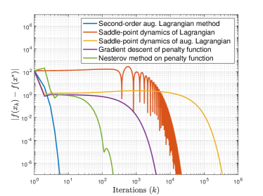
(a)

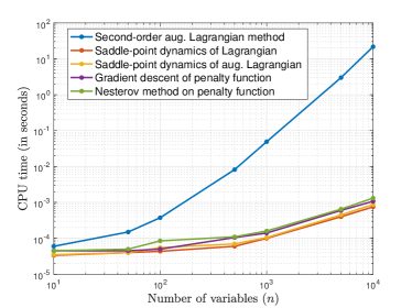
(b)

Figure 1: Performance comparison of the proposed algorithm (Nesterov’s acceleration on the penalty function) with the second-order augmented Lagrangian method [17], the saddle-point dynamics [9, 12] applied to the Lagrangian and the augmented Lagrangian, respectively, and the gradient descent of the penalty function. (a) shows the evolution of the error between the objective function and its optimal value for $n=50$ and (b) shows the computation time per iteration (note that the difference between second-order and first-order methods increases significantly with the problem dimension). For a desired level of accuracy, the proposed method outperforms the other methods when the number of iterations and the CPU time per iteration are jointly considered.

V Simulations

In this section, we show the effectiveness of the proposed approach through numerical simulations. We consider

$$\min_{x\in^{n}} \sum\limits_{i=1}^{n}\frac{1}{2}\beta_{i}x^{2}_{i}+\gamma_{i}\exp(x_{i})$$

  s.t. $$\sum\limits_{i=1}^{n}x_{i}=100,$$

where $\beta_{i}$, $\gamma_{i}\in\mathbb{R}_{>0}$. We evaluate different scenarios with values of $n$ as $10,50,100,500,1000,5000$ and $10000$. We take $\operatorname{\mathcal{D}}=\{x\in^{n}\;|\;\|x\|_{\infty}\leq 5,\sum\limits_{i=1}^{n}x_{i}-100\leq 50\}$. By Corollary IV.2, for $n=50$, the penalty function is strongly convex on $\operatorname{\mathcal{D}}$ with parameter $s=0.01$ for all $\epsilon\in(0,\bar{\epsilon}_{s}]$, where $\bar{\epsilon}_{s}=0.3603$. In our simulations, we use $\epsilon=10^{-1}$ and $\alpha=10^{-3}$, resp. Figure 1 compares the performance of the proposed method with the second-order augmented Lagrangian method [17], the saddle-point dynamics [9, 12] applied to the Lagrangian and the augmented Lagrangian, resp., and the gradient descent applied to the penalty function. Figure 1(a) shows the evolution of the error between the objective function and its optimal value for $n=50$. For the same level of accuracy, the number of iterations taken by the second-order augmented Lagrangian method is smaller by an order of magnitude compared to the proposed method. However, one should note that the second-order augmented Lagrangian method involves the inversion of Hessian, which becomes increasingly expensive as the number of variables increases (see also Remark 1). To illustrate this, Figure 1(b) shows the computation time per iteration of the algorithms in Matlab version 2018a running on a Macbook Pro with 2GHz i5 processor and 8 GB ram. The time taken by the first-order algorithms is about the same, and is smaller by several orders of magnitude (depending on the number of variables) than the second-order augmented Lagrangian method. When both aspects (number of iterations and computation time per iteration) are considered together, the proposed approach outperforms the other methods, especially if the problem dimension is large.

VI Conclusions

We have presented a fast approach for constrained convex optimization. We have provided sufficient conditions under which we can reformulate the original problem as the unconstrained optimization of a continuously differentiable convex penalty function. Our proposed approach is based on the accelerated gradient method given by Nesterov for unconstrained convex optimization, and has guaranteed convergence rate when the penalty function is (strongly) convex. From simulations, it is clear that in terms of computation time required to reach the desired accuracy, the proposed method performs the best compared to other state-of-the-art methods. Based on our previous work, this method is amenable to distributed optimization if, in the original problem, the objective function is separable and the constraint functions are locally expressible. Future work would explore the effect of the choice of penalty parameter on the convergence speed of the proposed strategy, the generalization of the conditions identified here to ensure the penalty function is (strongly) convex with inequality constraints, the extension of Nesterov’s accelerated gradient techniques to specific classes of non-convex functions (e.g., quasi-convex functions).

References

- [1] S. Boyd and L. Vandenberghe, Convex Optimization. Cambridge University Press, 2004.
- [2] Y. E. Nesterov, “A method of solving a convex programming problem with convergence rate ,” Soviet Mathematics Doklady, vol. 27, no. 2, pp. 372–376, 1983.
- [3] W. Su, S. Boyd, and E. J. Candés, “A differential equation for modeling Nesterov’s accelerated gradient method: theory and insights,” Journal of Machine Learning Research, vol. 17, pp. 1–43, 2016.
- [4] B. Shi, S. S. Du, W. Su, and M. I. Jordan, “Acceleration via symplectic discretization of high-resolution differential equations,” in Advances in Neural Information Processing Systems 32, H. Wallach, H. Larochelle, A. Beygelzimer, F. d’Alché Buc, E. Fox, and R. Garnett, Eds. Curran Associates, Inc., 2019, pp. 5744–5752.
- [5] Y. Nesterov, Lectures on Convex Optimization, 2nd ed., ser. Springer Optimization and Its Applications. Springer International Publishing, 2018, vol. 137.
- [6] T. Kose, “Solutions of saddle value problems by differential equations,” Econometrica, vol. 24, no. 1, pp. 59–70, 1956.
- [7] K. Arrow, L. Hurwitz, and H. Uzawa, Studies in Linear and Non-Linear Programming. Stanford, CA: Stanford University Press, 1958.
- [8] A. Cherukuri, B. Gharesifard, and J. Cortés, “Saddle-point dynamics: conditions for asymptotic stability of saddle points,” SIAM Journal on Control and Optimization, vol. 55, no. 1, pp. 486–511, 2017.
- [9] A. Cherukuri, E. Mallada, S. H. Low, and J. Cortés, “The role of convexity in saddle-point dynamics: Lyapunov function and robustness,” IEEE Transactions on Automatic Control, vol. 63, no. 8, pp. 2449–2464, 2018.
- [10] J. Chen and V. K. N. Lau, “Convergence analysis of saddle point problems in time varying wireless systems - control theoretical approach,” IEEE Transactions on Signal Processing, vol. 60, no. 1, pp. 443–452, 2012.
- [11] J. Cortés and S. K. Niederländer, “Distributed coordination for nonsmooth convex optimization via saddle-point dynamics,” Journal of Nonlinear Science, vol. 29, no. 4, pp. 1247–1272, 2019.
- [12] G. Qu and N. Li, “On the exponential stability of primal-dual gradient dynamics,” IEEE Control Systems Letters, vol. 3, no. 1, pp. 43–48, 2019.
- [13] D. Ding and M. R. Jovanović, “Global exponential stability of primal-dual gradient flow dynamics based on the proximal augmented Lagrangian,” in American Control Conference, Philadelphia, PA, July 2019, pp. 3414–3419.
- [14] S. S. Du and W. Hu, “Linear convergence of the primal-dual gradient method for convex-concave saddle point problems without strong convexity,” in The 22nd International Conference on Artificial Intelligence and Statistics, ser. Proceedings of Machine Learning Research, vol. 89, Naha, Okinawa, Japan, 2019, pp. 196–205.
- [15] W. Krichene, A. Bayen, and P. Bartlett, “Accelerated mirror descent in continuous and discrete time,” in Advances in Neural Information Processing Systems 28, C. Cortes, N. D. Lawrence, D. D. Lee, M. Sugiyama, and R. Garnett, Eds. Curran Associates, Inc., 2015, pp. 2845–2853.
- [16] P. E. Gill and D. P. Robinson, “A primal-dual augmented Lagrangian,” Computational Optimization and Applications, vol. 51, no. 1, pp. 1–25, 2012.
- [17] P. Armand and R. Omheni, “A globally and quadratically convergent primal-dual augmented Lagrangian algorithm for equality constrained optimization,” Optimization Methods and Software, vol. 32, no. 1, pp. 1–21, 2017.
- [18] N. K. Dhingra, S. Z. Khong, and M. R. Jovanović, “A second order primal-dual method for nonsmooth convex composite optimization,” IEEE Transactions on Automatic Control, 2017, submitted. https://arxiv.org/abs/1709.01610.
- [19] R. Fletcher, “A class of methods for nonlinear programming with termination and convergence properties,” in Integer and Nonlinear Programming, J. Abadie, Ed. Amsterdam: North-Holland, 1970, pp. 157–173.
- [20] T. Glad and E. Polak, “A multiplier method with automatic limitation of penalty growth,” Mathematical Programming, vol. 17, no. 1, pp. 140–155, 1979.
- [21] G. Di Pillo and L. Grippo, “Exact penalty functions in constrained optimization,” SIAM Journal on Control and Optimization, vol. 27, no. 6, pp. 1333–1360, 1989.
- [22] S. Lucidi, “New results on a continuously differentiable exact penalty function,” SIAM Journal on Optimization, vol. 2, no. 4, pp. 558–574, 1992.
- [23] G. Di Pillo, “Exact penalty methods,” in Algorithms for Continuous Optimization: The State of the Art, E. Spedicato, Ed. Dordrecht, The Netherlands: Kluwer Academic Publishers, 1994, pp. 209–253.
- [24] P. Srivastava and J. Cortés, “Distributed algorithm via continuously differentiable exact penalty method for network optimization,” in IEEE Conf. on Decision and Control, Miami Beach, FL, Dec. 2018, pp. 975–980.
- [25] R. T. Rockafellar, Convex Analysis. Princeton University Press, 1970.
- [26] D. P. Bertsekas, Nonlinear Programming, 2nd ed. Belmont, MA: Athena Scientific, 1999.
- [27] S. L. Campbell and C. D. Meyer, Generalized Inverses of Linear Transformations, ser. Classics in Applied Mathematics. Society for Industrial and Applied Mathematics, 2009.
- [28] F. H. Clarke, Optimization and Nonsmooth Analysis, ser. Canadian Mathematical Society Series of Monographs and Advanced Texts. Wiley, 1983.