Abstract

In this paper, as the first part of the third step of our study on developing data analysis procedures for using 3-dimensional information offered by directional direct Dark Matter detection experiments in the future, we present our double–Monte Carlo “scattering–by–scattering” simulation of the 3-dimensional elastic WIMP–nucleus scattering process, which can provide 3-D velocity information (the magnitude, the direction, and the incoming/scattering time) of each incident halo WIMP as well as the recoil direction and the recoil energy of the scattered target nucleus in different celestial coordinate systems. For readers’ reference, (animated) simulation plots with different WIMP masses and several frequently used target nuclei for all functionable underground laboratories can be found and downloaded on our online (interactive) demonstration webpage (http://www.tir.tw/phys/hep/dm/amidas-2d/).

1 Introduction

So far Weakly Interacting Massive Particles (WIMPs) $\chi$ arising in several extensions of the Standard Model of particle physics are still one of the most favorite candidates for cosmological Dark Matter (DM). In the last (more than) three decades, a large number of experiments has been built and is being planned to search for different WIMP candidates by direct detection of the scattering recoil energy of ambient WIMPs off target nuclei in low–background underground laboratory detectors (see Refs. [2, 3, 4, 5, 6, 7, 8] for reviews).

Besides non–directional direct detection experiments measuring only recoil energies deposited in detectors, the “directional” detection of Galactic DM particles has been proposed more than one decade to be a promising experimental strategy for discriminating signals from backgrounds by using additional 3-dimensional information (recoil tracks and/or head–tail senses) of (elastic) WIMP–nucleus scattering events (see Refs. [9, 10, 11, 12, 13, 14, 15, 16]). Several experimental collaborations investigate different detector materials and techniques [17, 18] and have achieved recently great progress [13, 14, 15].

(a)

(b)

Figure 1: The basic concepts of directional direct Dark Matter detection: (a) the diurnal modulation of the (main) incident direction of halo WIMPs, the so–called “directionality” of the WIMP wind, for a laboratory located in the Northern Hemisphere (in Summer); (b) except of the directionality of the WIMP wind, the event number of WIMP signals observed at a laboratory located in the Southern Hemisphere (in Winter) could also have the diurnal modulation caused by the Earth’s shielding of the WIMP flux. The darkened/lightened (left/right–hand) spheres indicate that the laboratory of interest is in the night/day.

The basic concept of directional direct Dark Matter detection is based on the rotation of the Earth. As sketched in Figs. 1, there are two kinds of possible “diurnal” modulation of WIMP signals to observe: the diurnal modulation of the (main) incident direction of halo WIMPs, the so–called “directionality” of the WIMP wind, as well as that of the number (scattering rate) of WIMP events caused by Earth’s shielding of the WIMP flux. Directional DM detection experiments aim originally hence, as the first step, to identify positive modulated anisotropic WIMP signals and discriminate them from theoretically (approximately) isotropic background events.

As the preparation for our future study on the development of data analysis procedures for using and/or combining 3-D information offered by directional detection experiments to, e.g., reconstruct the 3-dimensional WIMP velocity distribution, we develop step by step our double–Monte Carlo (MC) “scattering–by–scattering” simulation package for the 3-dimensional elastic WIMP–nucleus scattering process. In Ref. [19], we started with the Monte Carlo generation of the 3-D velocity of (incident) halo WIMPs in the Galactic coordinate system, including the magnitude, the direction, and the incoming/scattering time. Each generated 3-D WIMP velocity has then been transformed to the laboratory–independent (Ecliptic, Equatorial, and Earth) coordinate systems as well as to the laboratory–dependent (horizontal and laboratory) coordinate systems for further analyses [19, 20].

Now, we finally achieve the core part of our simulation package — the 3-D elastic WIMP–nucleus scattering process and can provide the recoil direction and then the recoil energy of the WIMP–scattered target nuclei event by event in different celestial coordinate systems, as pseudo–data for future investigations on analysis procedures and reconstruction methods. In this paper, we focus on the overall simulation procedure of 3-D elastic scattering by (generated and transformed) incident halo WIMPs, in particular, the validation of the 3-D recoil information of the WIMP–scattered target nuclei. Detailed studies on the angular distributions of the nuclear recoil direction/energy and the 3-dimensional effective velocity distribution of the incident WIMPs scattering off target nuclei will be presented separately in Refs. [21] and [22] respectively.

The remainder of this paper is organized as follows. In Sec. 2, we describe the overall workflow of our double–Monte Carlo scattering–by–scattering simulation procedure of 3-dimensional elastic WIMP–nucleus scattering. Then we review the MC generation of the 3-D velocity information of Galactic WIMPs as well as summarize the transformations between different celestial coordinate systems in Sec. 3. In Sec. 4, we introduce an incoming–WIMP coordinate system and describe in detail the validation criterion of our MC simulation of 3-D elastic WIMP–nucleus scattering events. We summarize in Sec. 5. The definitions of all celestial coordinate systems used in our simulation package and the transformation matrices between these coordinate systems will be given in Appendix.

2 Simulation workflow

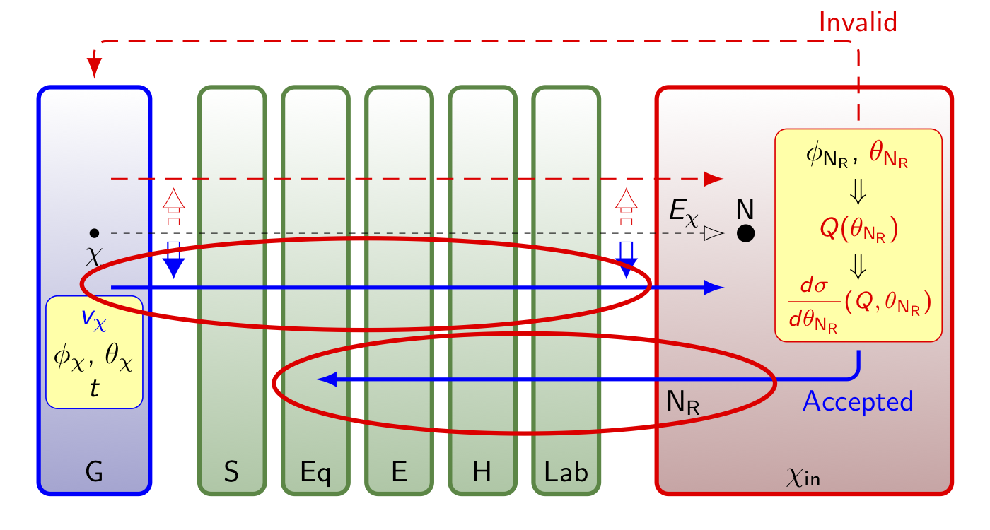
Figure 2: The workflow of our double–Monte Carlo simulation and data analysis procedure of 3-dimensional elastic WIMP–nucleus scattering. See the text for detailed descriptions.

In this section, we describe the overall workflow of our double–Monte Carlo simulation and data analysis procedure of 3-D elastic WIMP–nucleus scattering sketched in Fig. 2 in detail:

1. The 3-D velocity information of incident halo WIMPs (the magnitude and the direction as well as the incoming/scattering time) is MC generated according to a specified model of the Dark Matter halo in the Galactic coordinate system (the blue subframe), which will be described in Sec. 3.1.

2. The generated 3-D WIMP velocities will be transformed through the laboratory–independent (Ecliptic, Equatorial, and Earth) coordinate systems as well as the laboratory–dependent (horizontal and laboratory) coordinate systems (the green subframes, see Sec. 3.2) and at the end into the “incoming–WIMP” coordinate system (the red subframe), which definition will be given in Sec. 4.1.

3. In the incoming–WIMP coordinated system, the 3-D elastic WIMP–nucleus scattering process will also be MC simulated by generating an orientation of the scattering plane $\phi_{\rm N_{R},\chi_{in}}$ and an “equivalent” recoil angle $\theta_{\rm N_{R},\chi_{in}}$ (defined in Sec. 4.2). They define the recoil direction of the scattered target nucleus and the latter, combined with the transformed WIMP incident velocity, will then be used for estimating the transferred recoil energy to the target nucleus, $Q(\theta_{\rm N_{R},\chi_{in}})$, and the differential WIMP–nucleus scattering cross section with respect to the recoil angle, $d\sigma/d\theta_{\rm N_{R},\chi_{in}}(Q,\theta_{\rm N_{R},\chi_{in}})$, in our event validation criterion (see Sec. 4.2.1 for details).

4. The orientation of the scattering plane $\phi_{\rm N_{R},\chi_{in}}$ and the equivalent recoil angle $\theta_{\rm N_{R},\chi_{in}}$ of the accepted recoil events will be transformed (back) through all considered celestial coordinate systems (indicated by the lower solid blue arrow). All these 3-D recoil information of the scattered target nucleus accompanied with the corresponding recoil energy $Q$ as well as the 3-D velocity of the scattering WIMP in different coordinate systems (the upper solid blue arrow) will be recorded for further analyses [21, 22].

5. For the invalid cases, in which the estimated recoil energies are out of the experimental measurable energy window or suppressed by the validation criterion, the generated 3-D information on the incident WIMP (the lower dashed red arrow) (and that on the scattered nucleus) will be discarded and the generation/validation process of one WIMP scattering event will be restarted from the Galactic coordinate system (the upper dashed red arrow).

3 MC generation and transformations of incident WIMPs

For the completeness and readers’ reference, in this section, we review at first the generation of the 3-D WIMP velocity in the Galactic coordinate system and then summarize the transformations of the generated WIMP velocity through the laboratory–independent (Ecliptic, Equatorial, and Earth) coordinate systems as well as the laboratory–dependent (horizontal and laboratory) coordinate systems. While the definitions of all celestial coordinate systems used in our simulation package and the transformation matrices between these coordinate systems will be given in Appendix, discussions about our coordinate systems as well as the detailed derivations of the transformation matrices can be found in Ref. [19].

3.1 WIMP generation in the Galactic coordinate system

In this subsection, we review briefly the Monte Carlo generation of the 3-dimensional WIMP velocity (the magnitude and the direction as well as the incoming/scattering time) in the Galactic coordinate system.

3.1.1 Radial distribution of the 3-D WIMP velocity

For generating the radial component (magnitude) of the 3-D WIMP velocity in the Galactic coordinate system, we consider the simple Maxwellian velocity distribution truncated at the Galactic escape velocity [2]:

$$f_{\chi,{\rm G,r}}(v_{\chi,{\rm G}})=f_{1,{\rm Gau}}(v_{\chi,{\rm G}})=\left[\left(\frac{\sqrt{\pi}}{4}\right){\rm erf}\left(\frac{v_{\rm esc}}{v_{0}}\right)-\left(\frac{v_{\rm esc}}{2v_{0}}\right)e^{-v_{\rm esc}^{2}/v_{0}^{2}}\right]^{-1}\left(\frac{v_{\chi,{\rm G}}^{2}}{v_{0}^{3}}\right)e^{-v_{\chi,{\rm G}}^{2}/v_{0}^{2}}~{}\!,$$ (1)

for $v\leq v_{\rm esc}$, and $f_{\chi,{\rm G,r}}(v_{\chi,{\rm G}}>v_{\rm esc})=0$, where $v_{0}$ is the Solar orbital speed around the Galactic center and $492~{}{\rm km/s}<v_{\rm esc}<587~{}{\rm km/s}$ is the escape velocity from our Galaxy at the position of the Solar system [23].

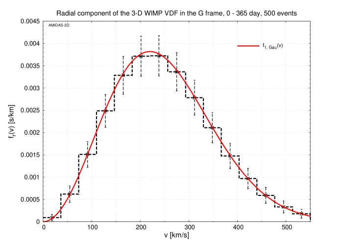
(a)

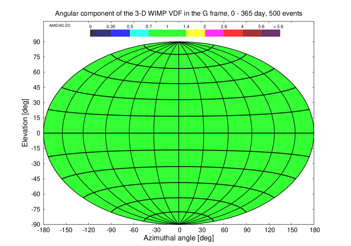
(b)

Figure 3: The radial (a) and the angular (b) components of the 3-D WIMP velocity in the Galactic coordinate system generated by Eq. (1) and Eqs. (2) and (3), respectively. The solid red curve (above) is the generating simple Maxwellian velocity distribution $f_{1,{\rm Gau}}(v_{v_{\chi,{\rm G}}})$ with $v_{0}=220$ km/s, while the dashed black histogram and the thin vertical dashed black lines show the (1$\sigma$ Poisson statistical uncertainties on the) number of the generated WIMP velocities. The horizontal color bar (below) indicates the mean value of the recorded event number (averaged over all simulated experiments) in each angular bin in unit of the all–sky average value (500 events/144 bins $\cong$ 3.47 events/bin here). See the text for further details.

In Fig. 3(a), we show the radial component of the 3-D WIMP velocity in the Galactic coordinate system generated by Eq. (1). 500 total events on average in one experiment (in one entire year) have been generated and binned into 15 bins. The solid red curve is the generating simple Maxwellian velocity distribution $f_{1,{\rm Gau}}(v_{v_{\chi,{\rm G}}})$ with the Solar Galactic orbital velocity $v_{0}=220$ km/s, while the dashed black histogram and the thin vertical dashed black lines show the (1$\sigma$ Poisson statistical uncertainties on the) number of the generated WIMP velocities. The Galactic escape velocity has been set as $v_{\rm esc}=550$ km/s. 5,000 experiments have been simulated.

3.1.2 Angular distribution of the 3-D WIMP velocity

Since the simplest model of the Galactic Dark Matter halo is assumed to be isothermal, spherical and isotropic, the angular distribution (direction) of the 3-D WIMP velocity in the Galactic coordinate system has been considered to be isotropic and thus the azimuthal angle $\phi$ and the elevation $\theta$ are generated with constant probabilities:

$$f_{\chi,{\rm G},\phi}(\phi_{\rm\chi,G})=1~{}\!,~{}~{}~{}~{}~{}~{}~{}~{}~{}~{}\phi_{\rm\chi,G}\in(-\pi,~{}\pi]~{}\!,$$ (2)

and

$$f_{\chi,{\rm G},\theta}(\theta_{\rm\chi,G})=1~{}\!,~{}~{}~{}~{}~{}~{}~{}~{}~{}~{}\theta_{\rm\chi,G}\in[-\pi/2,~{}\pi/2]~{}\!.$$ (3)

In Fig. 3(b), we show the angular component of the 3-D WIMP velocity in the Galactic coordinate system generated by Eqs. (2) and (3). 500 total events on average (in one experiment in one entire year) have been binned into 12 $\times$ 12 bins for the azimuthal angle and the elevation, respectively. The horizontal color bar on the top of the plot indicates the mean value of the recorded event number (averaged over all simulated experiments) in each angular bin in unit of the all–sky average value (500 events/144 bins $\cong$ 3.47 events/bin here).

3.1.3 Incoming/scattering time of 3-D WIMP–nucleus scattering events

Since, in the Galactic point of view, WIMP–nucleus scattering events should be observed randomly and constantly, we consider a constant probability for generating the UTC (Coordinated Universal Time) incoming/scattering time of the recorded WIMP signals:

$$f_{t}(t)=1~{}\!,~{}~{}~{}~{}~{}~{}~{}~{}~{}~{}t\in[t_{\rm start},~{}t_{\rm end}]~{}\!.$$ (4)

For example, for generating the WIMP events shown in Figs. 3, the observation period has been set as $[t_{\rm start},~{}t_{\rm end}]=[0,365~{}{\rm day}]$.

3.1.4 Observation periods for annual modulations

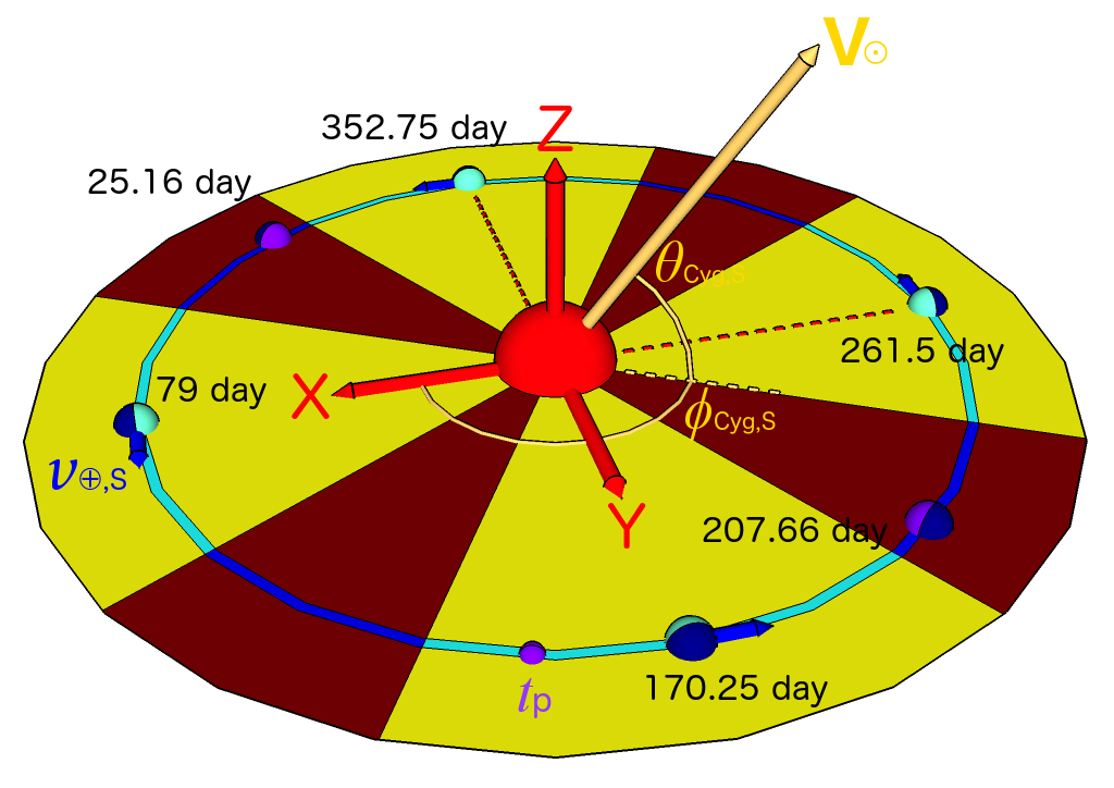
(a)

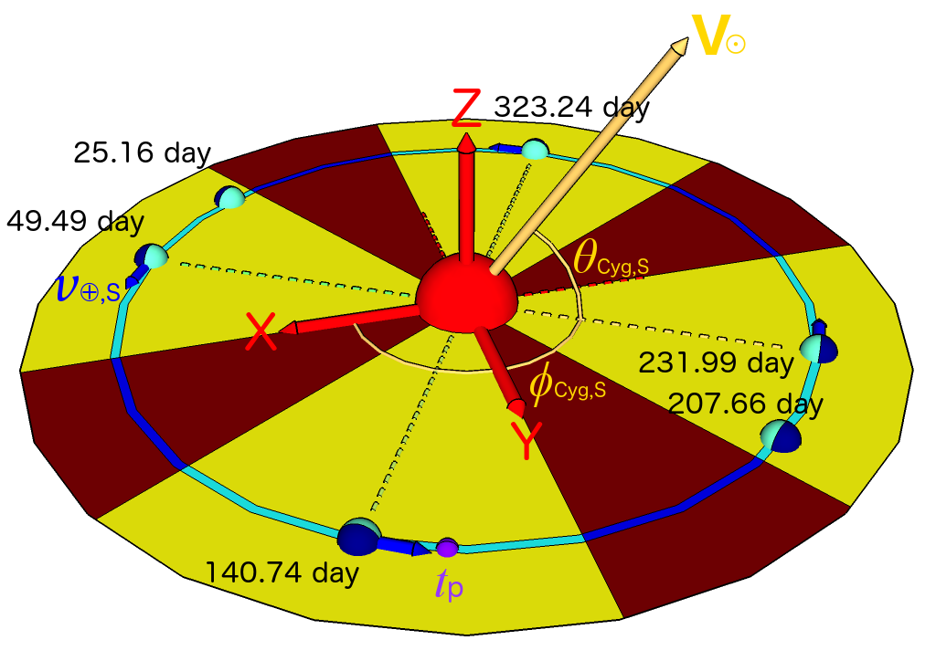
(b)

Figure 4: Two options for the 60-day ($\pm$ 30 days) observation periods (lightened areas) considered for demonstrating annual modulations (listed in Table 1): (a) four normal seasons and (b) four “advanced” seasons. While the golden arrows indicate the moving direction of the Solar system towards the CYGNUS constellation with the velocity of $|{\bf v}_{\rm\odot,G}|\simeq 220$ km/s, the short dark–blue arrows (in front of the Earths) indicate the (average) orbital velocity of the Earth, $|{\bf v}_{\rm\oplus,S}|\cong 29.79$ km/s, on the central dates of the observation periods. Additionally, the Earths without the velocity arrows indicate the locations considered for demonstrating diurnal modulations (see also Fig. 5) and the small purple points at the bottom of the sketches indicate the Earth’s location around June 2nd ($t_{\rm p}=152.5$ day) [24]. See Appendix A.1 and Ref. [19] for further details.

Option	Central date (day)	Period (day)
One entire year	—	0 – 365
Four normal seasons	79.0	49.0 – 109.0
	170.25	140.25 – 200.25
	261.50	231.50 – 291.50
	352.75	322.75 – 382.75 (= 17.75)
Four advanced seasons	49.49	19.49 – 79.49
	140.74	110.74 – 170.74
	231.99	201.99 – 261.99
	323.24	293.24 – 353.24
For diurnal modulations	207.66	177.66 – 237.66
	390.16 (= 25.16)	360.16 – 420.16 (= 55.16)

Table 1: Four options for the observation periods in a 365-day year considered in our simulation package. Note that the last option is only for demonstrating diurnal modulations.

As discussed in detail in Ref. [19], two options for the observation periods have been considered for demonstrating the annual modulations of e.g. the angular distributions of the WIMP velocity (flux) [19] and the (average) kinetic energy [20] (sketched in Figs. 4 and listed in Table 1). The first one is the natural choice of four normal seasons with the central dates on the March 21st (79.0 day), the June 20th (170.25 day), the September 19th (261.50 day), and the December 19th (352.75 day), respectively.

Meanwhile, considering that the relative velocity of the Earth to the Galactic Dark Matter halo should be the maximum (minimum), when its orbital velocity is (anti–)parallel to the projection of the direction of the Solar movement on the Ecliptic plane around the 21st of May (140.74 day) (the 20th of November, 323.24 day), the second option is four “advanced” seasons ($\sim$ 30 days earlier) with the central dates on the February 19th (49.49 day), the May 21st (140.74 day), the August 20th (231.99 day), and the November 20th (323.24 day), respectively. For each season of these two options, we considered a 60-day ($\pm$ 30 days) observation period and each pair of the corresponding season has thus an overlap of around 30 days.

3.1.5 Daily shifts for diurnal modulations

Option	Central time (hour)	Interval (hour)
One entire day	—	0 – 24
Four daily shifts	0	0 – 2, 22 – 24
	6	4 – 8
	12	10 – 14
	18	16 – 20

Table 2: Two options for the observation intervals in a 24-hour day considered in our simulation package.

For demonstrating (the originally proposed) diurnal modulations, we considered four observation intervals of 4 hours ($\pm 2$ hours) at the central (local, not the UTC) times of 0, 6, 12, and 18 o’clock, respectively (listed in Table 2), in the 60-day periods centered on the January 26th (25.16 = 390.16 day) and the July 27th (207.66 day), respectively (sketched in Figs. 4 and 5, see Ref. [19] for details).

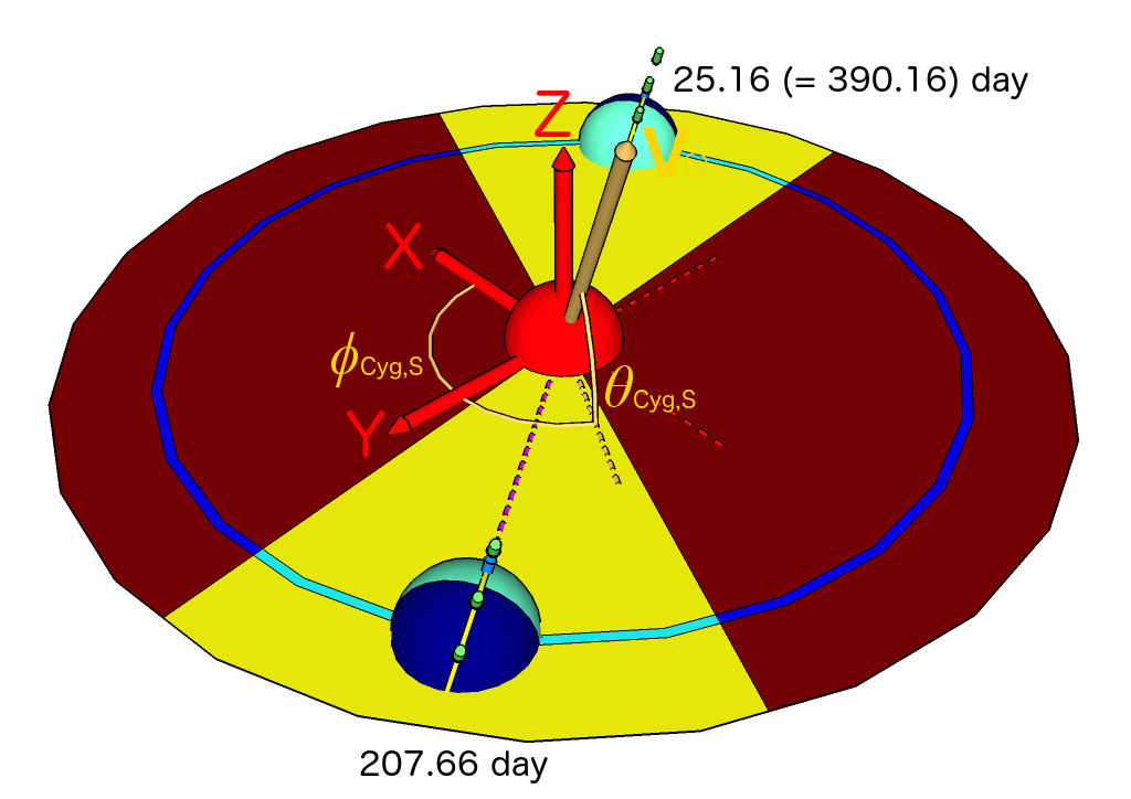
Figure 5: Two options for the 60-day ($\pm$ 30 days) observation periods (lightened areas) considered for demonstrating diurnal modulations (listed in Table 1), on which the (light–green) theoretical main direction of incident halo WIMPs points straightly to the (yellow) Prime Meridian in the night or the day. See Appendix A.1 and Ref. [19] for further details.

3.2 Transformations of the 3-D velocity

In this subsection, we summarize the transformations of the generated 3-D WIMP velocity as well as the recoil direction of the scattered target nucleus between different celestial coordinate systems. The analytic and/or numerical forms of the needed transformation matrices will be summarized in Appendix.

3.2.1 Between the Galactic and the Ecliptic coordinate systems

In our simulation package, the 3-D WIMP velocity in the Ecliptic coordinate system ${\bf v}_{\chi,{\rm S}}$ transformed from the generated 3-D velocity in the Galactic coordinate system ${\bf v}_{\chi,{\rm G}}(v_{\rm\chi,G,x},v_{\rm\chi,G,y},v_{\rm\chi,G,z})={\bf v}_{\chi,{\rm G}}(v_{\chi,{\rm G}},\phi_{\rm\chi,G},\theta_{\rm\chi,G})$ can be given by

$${\bf v}_{\chi,{\rm S}}={\bf M}_{\rm G\to S}({\bf v}_{\chi,{\rm G}}-{\bf v}_{\rm\odot,G})~{}\!,$$ (5a)

with the transformation matrix ${\bf M}_{\rm G\to S}$ given in Eq. (A23a) and

$${\bf v}_{\rm\odot,G}\simeq\left[\begin{array}[]{c}33.58~{}{\rm km/s}\\ 217.41~{}{\rm km/s}\\ 2.32~{}{\rm km/s}\\ \end{array}\right]_{\rm G}$$ (6)

is the moving velocity of the Solar system (towards the CYGNUS constellation) in the Galactic coordinate system [19]. Conversely, for the recoil direction of the WIMP–scattered target nucleus, we can use

$${\bf v}_{\rm N_{R},G}={\bf M}_{\rm S\to G}{\bf v}_{\rm N_{R},S}+{\bf v}_{\rm\odot,G}~{}\!,$$ (5b)

where the transformation matrix ${\bf M}_{\rm S\to G}$ is given in Eq. (A23b).

3.2.2 Between the Ecliptic and the Equatorial coordinate systems

Similar to Eqs. (5a) and (5b), the 3-D WIMP velocity in the Equatorial coordinate system ${\bf v}_{\chi,{\rm Eq}}$ transformed from the transformed 3-D velocity in the Ecliptic coordinate system ${\bf v}_{\chi,{\rm S}}$ can be given by

$${\bf v}_{\chi,{\rm Eq}}={\bf M}_{\rm S\to Eq}\Big{[}{\bf v}_{\chi,{\rm S}}-{\bf v}_{\rm\oplus,S}(t)\Big{]}~{}\!,$$ (7a)

where $t$ is the UTC incoming/scattering time of the WIMP event, the transformation matrix ${\bf M}_{\rm S\to Eq}$ is given in Eq. (A7a) and

$${\bf v}_{\rm\oplus,S}(t)=v_{\rm\oplus,S}\left[\begin{array}[]{c}-\sin(\psi_{\rm yr}(t))\\ \cos(\psi_{\rm yr}(t))\\ 0\\ \end{array}\right]_{\rm S}~{}\!,$$ (8)

is the time–dependent Earth’s orbital velocity around the Sun in the Ecliptic coordinate system. Here the Earth’s orbital speed can be estimated as [23]

$$v_{\rm\oplus,S}\cong 29.79~{}{\rm km/s}~{}\!,$$ (9)

and the angle swept by the connection between the Solar and the Earth’s centers from the day of the vernal equinox (the 79th day) can be expresses by

$$\psi_{\rm yr}(t)\equiv\frac{2\pi}{365}\Big{[}(t-t_{\rm PM})-79.0\Big{]}~{}\!,$$ (10)

where $t_{\rm PM}$ indicates the fractional part of the UTC incoming/scattering time $t$ in unit of day. Conversely, for the recoil direction of the WIMP–scattered target nucleus, we have

$${\bf v}_{\rm N_{R},S}={\bf M}_{\rm Eq\to S}{\bf v}_{\rm N_{R},Eq}+{\bf v}_{\rm\oplus,S}(t)~{}\!,$$ (7b)

with the transformation matrix ${\bf M}_{\rm Eq\to S}$ given in Eq. (A7b).

3.2.3 Between the Equatorial and the Earth coordinate systems

In our simulation package, the transformations of the 3-D (WIMP) velocity at the incoming/scattering time $t$ between the Equatorial and the Earth coordinate systems are pure rotations, which can be given by

$${\bf v}_{\chi,{\rm E}}={\bf M}_{\rm Eq\to E}(t){\bf v}_{\chi,{\rm Eq}}~{}\!,$$ (11a)

and, conversely, one has

$${\bf v}_{\rm N_{R},Eq}={\bf M}_{\rm E\to Eq}(t){\bf v}_{\rm N_{R},E}~{}\!,$$ (11b)

with the time–dependent transformation matrices ${\bf M}_{\rm Eq\to E}(t)$ and ${\bf M}_{\rm E\to Eq}(t)$ given in Eqs. (A27a) and (A27b), respectively.

3.2.4 Between the Earth and the horizontal coordinate systems

By definition, the transformations of the 3-D (WIMP) velocity (at the UTC incoming/scattering time $t$) between the Earth and the horizontal coordinate systems are pure time–independent rotations, which can be given by

$${\bf v}_{\chi,{\rm H}}={\bf M}_{\rm E\to H}(\phi_{\rm Lab},\theta_{\rm Lab}){\bf v}_{\chi,{\rm E}}~{}\!,$$ (12a)

and, conversely,

$${\bf v}_{\rm N_{R},E}={\bf M}_{\rm H\to E}(\phi_{\rm Lab},\theta_{\rm Lab}){\bf v}_{\rm N_{R},H}~{}\!,$$ (12b)

where the transformation matrices ${\bf M}_{\rm E\to H}(\phi_{\rm Lab},\theta_{\rm Lab})$ and ${\bf M}_{\rm H\to E}(\phi_{\rm Lab},\theta_{\rm Lab})$ depending only on the longitude and the latitude of the location of the considered laboratory $(\phi_{\rm Lab},\theta_{\rm Lab})$ are given in Eqs. (A30a) and (A30b).

3.2.5 Between the horizontal and the laboratory coordinate systems

Similar to Eqs. (12a) and (12b), the transformations (pure rotations) of the 3-D (WIMP) velocity at the incoming/scattering time $t$ between the horizontal and the laboratory coordinate systems can be given by

$${\bf v}_{\chi,{\rm Lab}}={\bf M}_{\rm H\to Lab}(t,\phi_{\rm Lab},\theta_{\rm Lab}){\bf v}_{\chi,{\rm H}}~{}\!,$$ (13a)

and, conversely,

$${\bf v}_{\rm N_{R},H}={\bf M}_{\rm Lab\to H}(t,\phi_{\rm Lab},\theta_{\rm Lab}){\bf v}_{\rm N_{R},Lab}~{}\!,$$ (13b)

where the transformation matrices ${\bf M}_{\rm H\to Lab}(t,\phi_{\rm Lab},\theta_{\rm Lab})$ and ${\bf M}_{\rm Lab\to H}(t,\phi_{\rm Lab},\theta_{\rm Lab})$ depending not only on the longitude and the latitude of the laboratory location $(\phi_{\rm Lab},\theta_{\rm Lab})$ but also on the incoming/scattering time $t$ ($t_{\rm PM}$) are given in Eqs. (A41a) and (A44b).

3.2.6 Between the laboratory and the incoming–WIMP coordinate systems

Finally, for the transformation (pure rotation) of the recoil direction of the WIMP–scattered target nucleus generated in the incoming–WIMP coordinate system to the laboratory coordinate system, one has

$${\bf v}_{\rm N_{R},Lab}={\bf M}_{\rm\chi_{in}\to Lab}(\phi_{\rm\chi,Lab},\theta_{\rm\chi,Lab}){\bf v}_{\rm N_{R},\chi_{in}}~{}\!,$$ (14)

where the transformation matrix ${\bf M}_{\rm\chi_{in}\to Lab}(\phi_{\rm\chi,Lab},\theta_{\rm\chi,Lab})$ depending on the azimuthal angle $\phi_{\rm\chi,Lab}$ and the elevation $\theta_{\rm\chi,Lab}$ of the incident direction of the scattering WIMP measured in the laboratory coordinate system is given in Eq. (A48a).

4 MC generation of 3-D elastic WIMP–nucleus scattering events

As described in Sec. 2, each generated 3-D WIMP velocity will be transformed through different celestial coordinate systems and at the end into the “incoming–WIMP” ($\chi_{\rm in}$) coordinate system. In this section, we describe then the core part of our simulation procedure: the generation of 3-D elastic WIMP–nucleus scattering events in the incoming–WIMP coordinate system.

We give at first our definition of the incoming–WIMP coordinate system as well as those of (the orientation of) the scattering plane and the (equivalent) recoil angle. Then we discuss the validation criterion in our Monte Carlo simulation by taking into account the cross section (nuclear form factor) suppression in detail.

4.1 Definition of the incoming–WIMP coordinate system

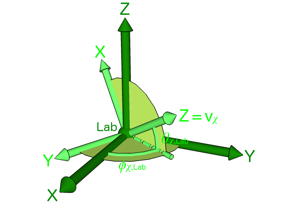
Figure 6: The definition of the (light–green) incoming–WIMP coordinate system in the (dark–green) laboratory coordinate system. The ${\bf Z}_{\chi_{\rm in}}$–axis is defined as usual as the direction of the incident velocity of the incoming WIMP ${\bf v}_{\chi}$. $\phi_{\rm\chi,Lab}$ and $\theta_{\rm\chi,Lab}$ indicate the azimuthal angle and the elevation of the direction of ${\bf v}_{\chi}$ measured in the laboratory coordinate system, respectively. The ${\bf X}_{\chi_{\rm in}}$–axis is perpendicular to the ${\bf Z}_{\chi_{\rm in}}$–axis and lies on the ${\bf Z}_{\rm Lab}$–${\bf Z}_{\chi_{\rm in}}$ plane. Then the ${\bf Y}_{\chi_{\rm in}}$–axis is defined by the right–handed convention.

In Fig. 6, we sketch the definition of the (light–green) incoming–WIMP coordinate system in the (dark–green) laboratory coordinate system. Note that, practically, the center of the incoming–WIMP coordinate system is at the position of the scattered target nucleus before scattering (see Fig. 7). The ${\bf Z}_{\chi_{\rm in}}$–axis is defined as usual as the direction of the incident velocity of the incoming WIMP ${\bf v}_{\chi}$. $\phi_{\rm\chi,Lab}$ and $\theta_{\rm\chi,Lab}$ indicate the azimuthal angle and the elevation of the direction of ${\bf v}_{\chi}$ measured in the laboratory coordinate system, respectively. The ${\bf X}_{\chi_{\rm in}}$–axis is perpendicular to the ${\bf Z}_{\chi_{\rm in}}$–axis and lies on the ${\bf Z}_{\rm Lab}$–${\bf Z}_{\chi_{\rm in}}$ plane. Then the ${\bf Y}_{\chi_{\rm in}}$–axis is defined by the right–handed convention. Note that the ${\bf Y}_{\chi_{\rm in}}$–axis lies always on the ${\bf X}_{\rm Lab}$–${\bf Y}_{\rm Lab}$ plane, since it is perpendicular to the ${\bf X}_{\chi_{\rm in}}$–${\bf Z}_{\rm Lab}$–${\bf Z}_{\chi_{\rm in}}$ plane.

Note also that, in our Monte Carlo simulation of 3-D elastic WIMP–nucleus scattering events, the velocity (incident direction) of halo WIMPs in the laboratory and the Equatorial coordinate systems as well as the ${\bf Z}_{\chi_{\rm in}}$–axis of the incoming–WIMP coordinate system are not fixed as from the direction of the CYGNUS constellation. Interested readers can refer to Ref. [19] for the detailed discussions about (the annual and the diurnal modulations of) the anisotropy of the angular distributions of the 3-D WIMP velocity (flux) in the laboratory and the Equatorial coordinate systems.

4.2 Generation of nuclear recoil directions

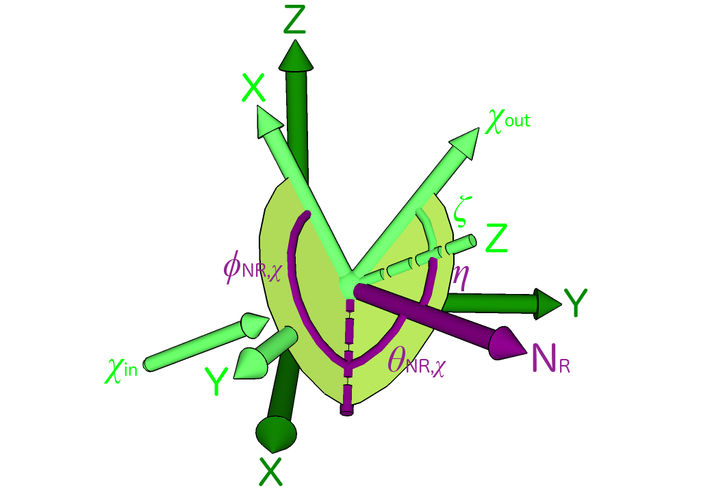
Figure 7: A 3-D elastic WIMP–nucleus scattering event in the (light–green) incoming–WIMP and the (dark–green) laboratory coordinate systems. $\zeta$ and $\eta$ are the scattering angle of the outgoing WIMP $\chi_{\rm out}$ and the recoil angle of the scattered target nucleus N_R measured in the incoming–WIMP coordinate system of this single scattering event, respectively. While the azimuthal angle of the recoil direction of the scattered nucleus N_R in this incoming–WIMP coordinate system, $\phi_{\rm N_{R},\chi_{in}}$, indicates the orientation of the scattering plane, the elevation of the recoil direction of N_R, $\theta_{\rm N_{R},\chi_{in}}$, is namely the complementary angle of the recoil angle $\eta$.

At first, we sketch in Fig. 7 the process of one single 3-D elastic WIMP–nucleus scattering event: $\chi_{\rm in/out}$ indicate the incoming and the outgoing WIMPs, respectively. While $\zeta$ indicates the scattering angle of the outgoing WIMP $\chi_{\rm out}$ (measured from the ${\bf Z}_{\chi_{\rm in}}$–axis), $\eta$ is the recoil angle of the scattered target nucleus N_R.

It can be found firstly that, according to our definition of the incoming–WIMP coordinate system, the orientation of the (${\bf v}_{\chi_{\rm out}}$–${\bf Z}_{\chi_{\rm in}}$–${\bf v}_{\rm N_{R}}$) scattering plane of this single scattering event (in the incoming–WIMP coordinate system) can be specified by the azimuthal angle of the recoil direction of the scattered nucleus, $\phi_{\rm N_{R},\chi_{in}}$, which should be azimuthal symmetric around the ${\bf Z}_{\chi_{\rm in}}$–axis and is thus generated with a constant probability in our simulation package:

$$f_{{\rm N_{R}},\chi_{\rm in},\phi}(\phi_{\rm N_{R},\chi_{in}})=1~{}\!,~{}~{}~{}~{}~{}~{}~{}~{}~{}~{}\phi_{\rm N_{R},\chi_{in}}\in(-\pi,~{}\pi]~{}\!.$$ (15)

Meanwhile, Fig. 7 shows also that the elevation of the recoil direction of the scattered nucleus, $\theta_{\rm N_{R},\chi_{in}}$, is namely the complementary angle of the recoil angle $\eta$:

$$\theta_{\rm N_{R},\chi_{in}}=\frac{\pi}{2}-\eta~{}\!.$$ (16)

Hence, in our simulation package, we use

$$\theta_{\rm N_{R},\chi_{in}}\in[0,~{}\pi/2]$$ (17)

as the “equivalent” recoil angle.

In contrast to the simple constant generating probability $f_{{\rm N_{R}},\chi_{\rm in},\phi}(\phi_{\rm N_{R},\chi_{in}})$ given in Eq. (15) for the orientation of the scattering plane $\phi_{\rm N_{R},\chi_{in}}$, the generating probability distribution of the recoil angle $\theta_{\rm N_{R},\chi_{in}}$ is more complicated and crucial. Below we discuss the cross section (nuclear form factor) suppression on the probability distribution of $\theta_{\rm N_{R},\chi_{in}}$ in detail.

4.2.1 Validation of 3-D elastic WIMP–nucleus scattering events

For one WIMP event generated in the Galactic coordinate system and transformed step by step into the laboratory coordinate system with the velocity of ${\bf v}_{\chi}(v_{\chi,{\rm Lab}},\phi_{\rm\chi,Lab},\theta_{\rm\chi,Lab})$, the kinetic energy can be given by

$$E_{\chi}=\frac{1}{2}m_{\chi}|{\bf v}_{\chi}|^{2}=\frac{1}{2}m_{\chi}v_{\chi,{\rm Lab}}^{2}~{}\!.$$ (18)

Then the recoil energy of the scattered target nucleus in the incoming–WIMP coordinate system can be estimated by the recoil angle $\eta$ or the equivalent recoil angle $\theta_{\rm N_{R},\chi_{in}}$ as

$$Q=\left[\frac{4m_{\chi}m_{\rm N}}{(m_{\chi}+m_{\rm N})^{2}}~{}\!\cos^{2}(\eta)\right]E_{\chi}=\left[\left(\frac{2m_{\rm r,N}^{2}}{m_{\rm N}}\right)v_{\chi,{\rm Lab}}^{2}\right]\sin^{2}(\theta_{\rm N_{R},\chi_{in}})~{}\!,$$ (19)

where

$$m_{\rm r,N}\equiv\frac{m_{\chi}m_{\rm N}}{m_{\chi}+m_{\rm N}}$$ (20)

is the reduced mass of the WIMP mass $m_{\chi}$ and that of the target nucleus $m_{\rm N}$. From Eq. (19), one can get that

$$\frac{dQ}{d\theta_{\rm N_{R},\chi_{in}}}=\left[\left(\frac{2m_{\rm r,N}^{2}}{m_{\rm N}}\right)v_{\chi,{\rm Lab}}^{2}\right]\sin(2\theta_{\rm N_{R},\chi_{in}})~{}\!.$$ (21)

Hence, the differential cross section $d\sigma$ given by the absolute value of the momentum transfer from the incident WIMP to the recoiling target nucleus,

$$q=|{\bf q}|=\sqrt{2m_{\rm N}Q}~{}\!,$$ (22)

can be obtained as [2]

$$d\sigma=\frac{1}{v_{\chi,{\rm Lab}}^{2}}\left(\frac{\sigma_{0}}{4m_{\rm r,N}^{2}}\right)F^{2}(q)~{}\!dq^{2}=\sigma_{0}F^{2}(Q)\sin(2\theta_{\rm N_{R},\chi_{in}})~{}\!d\theta_{\rm N_{R},\chi_{in}}~{}\!.$$ (23)

Then the differential WIMP–nucleus scattering cross section with respect to the recoil angle $\theta_{\rm N_{R},\chi_{in}}$ can generally be given by

$$\frac{d\sigma}{d\theta_{\rm N_{R},\chi_{in}}}=\bigg{[}\sigma_{0}^{\rm SI}F_{\rm SI}^{2}(Q)+\sigma_{0}^{\rm SD}F_{\rm SD}^{2}(Q)\bigg{]}\sin(2\theta_{\rm N_{R},\chi_{in}})~{}\!.$$ (24)

Here $\sigma_{0}^{\rm(SI,SD)}$ are the spin–independent (SI)/spin–dependent (SD) total cross sections ignoring the form factor suppression and $F_{\rm(SI,SD)}(Q)$ indicate the elastic nuclear form factors corresponding to the SI/SD WIMP interactions, respectively. Remind that the recoil energy $Q$ is the function of the recoil angle $\theta_{\rm N_{R},\chi_{in}}$ given by Eq. (19).

Finally, taking into account the proportionality of the WIMP flux to the incident velocity, the generating probability distribution of the recoil angle $\theta_{\rm N_{R},\chi_{in}}$, which is proportional to the scattering event rate of incident halo WIMPs with an incoming velocity $v_{\chi,{\rm Lab}}$ off target nuclei going into recoil angles of $\theta_{\rm N_{R},\chi_{in}}\pm d\theta_{\rm N_{R},\chi_{in}}/2$ with recoil energies of $Q\pm dQ/2$, can generally be given by

$$f_{{\rm N_{R}},\chi_{\rm in},\theta}(\theta_{\rm N_{R},\chi_{in}}) = \left(\frac{v_{\chi,{\rm Lab}}}{v_{\chi,{\rm cutoff}}}\right)\left(\frac{d\sigma}{d\theta_{\rm N_{R},\chi_{in}}}\right)$$ (25)

$$= \left(\frac{v_{\chi,{\rm Lab}}}{v_{\chi,{\rm cutoff}}}\right)\bigg{[}\sigma_{0}^{\rm SI}F_{\rm SI}^{2}(Q)+\sigma_{0}^{\rm SD}F_{\rm SD}^{2}(Q)\bigg{]}\sin(2\theta_{\rm N_{R},\chi_{in}})~{}\!,$$

where $v_{\chi,{\rm cutoff}}\simeq 800$ km/s is a cut–off velocity of incident halo WIMPs in the laboratory coordinate system.

4.2.2 WIMP–nucleus cross sections and nuclear form factors

For the SI scalar WIMP interaction, the zero–momentum–transfer cross section in Eq. (24) has been given by [2]

$$\sigma_{0}^{\rm SI}=\left(\frac{4}{\pi}\right)m_{\rm r,N}^{2}\Big{[}Zf_{\rm p}+(A-Z)f_{\rm n}\Big{]}^{2}=A^{2}\left(\frac{m_{\rm r,N}}{m_{\rm r,p}}\right)^{2}\sigma_{\chi{\rm p}}^{\rm SI}~{}\!.$$ (27)

Here $m_{\rm r,p}$ is the reduced mass of the WIMP mass $m_{\chi}$ and the proton mass $m_{\rm p}$, $Z$ is the atomic number of the target nucleus, i.e. the number of protons, $A$ is the atomic mass number, $A-Z$ is then the number of neutrons, $f_{\rm(p,n)}$ are the effective scalar couplings of WIMPs on protons p and on neutrons n, respectively, and

$$\sigma_{\chi{\rm p}}^{\rm SI}=\left(\frac{4}{\pi}\right)m_{\rm r,p}^{2}|f_{\rm p}|^{2}$$ (28)

is the SI scalar WIMP–nucleon cross section. The theoretical prediction for the lightest supersymmetric neutralino: the scalar couplings are approximately the same on protons and on neutrons, $f_{\rm n}\simeq f_{\rm p}$, has been adopted here and the tiny mass difference between a proton and a neutron has been neglected.

On the other hand, the SD axial–vector WIMP–nucleus cross section in Eq. (24) can be expressed as [2]

$$\sigma_{0}^{\rm SD} = \left(\frac{32}{\pi}\right)G_{F}^{2}~{}\!m_{\rm r,N}^{2}\left(\frac{J+1}{J}\right)\Big{[}\langle{\textstyle{S_{\rm p}}}\rangle a_{\rm p}+\langle{\textstyle{S_{\rm n}}}\rangle a_{\rm n}\Big{]}^{2}$$ (29)

$$= \frac{4}{3}\left(\frac{J+1}{J}\right)\left(\frac{m_{\rm r,N}}{m_{\rm r,p}}\right)^{2}\left[\langle{\textstyle{S_{\rm p}}}\rangle+\langle{\textstyle{S_{\rm n}}}\rangle\left(\frac{a_{\rm n}}{a_{\rm p}}\right)\right]^{2}\sigma_{\chi{\rm p}}^{\rm SD}~{}\!.$$

Here $G_{F}$ is the Fermi constant, $J$ is the total spin of the target nucleus, $\langle{\textstyle{S_{\rm(p,n)}}}\rangle$ are the expectation values of the proton and neutron group spins (see Table 3 for the list of the default spin values of the nuclei used in our simulation package), $a_{\rm(p,n)}$ are the effective SD axial–vector WIMP couplings on protons and on neutrons, respectively, and the SD WIMP cross section on protons or on neutrons can be given by

$$\sigma_{\chi{\rm(p,n)}}^{\rm SD}=\left(\frac{24}{\pi}\right)G_{F}^{2}~{}\!m_{\rm r,(p,n)}^{2}|a_{\rm(p,n)}|^{2}~{}\!.$$ (30)

Isotope	$Z$	$J$	$\langle{\textstyle{S_{\rm p}}}\rangle$	$\langle{\textstyle{S_{\rm n}}}\rangle$	Natural abundance (%)
${}^{7}{\rm Li}$	3	3/2	0.497	0.004	92.41
${}^{17}{\rm O}$	8	5/2	0	0.495	0.038
${}^{19}{\rm F}$	9	1/2	0.441	$-$0.109	100
${}^{23}{\rm Na}$	11	3/2	0.248	0.020	100
${}^{27}{\rm Al}$	13	5/2	0.343	0.030	100
${}^{29}{\rm Si}$	14	1/2	$-$0.002	0.130	4.68
${}^{35}{\rm Cl}$	17	3/2	$-$0.059	$-$0.011	75.78
${}^{37}{\rm Cl}$	17	3/2	$-$0.058	0.050	24.22
${}^{39}{\rm K}$	19	3/2	$-$0.180	0.050	93.26
${}^{73}{\rm Ge}$	32	9/2	0.030	0.378	7.73
${}^{93}{\rm Nb}$	41	9/2	0.460	0.080	100
${}^{125}{\rm Te}$	52	1/2	0.001	0.287	7.07
${}^{127}{\rm I}$	53	5/2	0.309	0.075	100
${}^{129}{\rm Xe}$	54	1/2	0.028	0.359	26.44
${}^{131}{\rm Xe}$	54	3/2	$-$0.009	$-$0.227	21.18
${}^{133}{\rm Cs}$	55	7/2	$-$0.370	0.003	100
${}^{183}{\rm W}$	74	1/2	0	$-$0.031	14.31

Table 3: List of the default spin values of the nuclei used in our simulation package [25, 26, 27, 28, 29].

Substituting Eqs. (27) and (29) into Eq. (25), the validation criterion of our 3-D elastic WIMP–nucleus scattering simulation can be expressed as

$$f_{{\rm N_{R}},\chi_{\rm in},\theta}(\theta_{\rm N_{R},\chi_{in}})$$ (31)

$$= \left(\frac{v_{\chi,{\rm Lab}}}{v_{\chi,{\rm cutoff}}}\right)\left(\frac{m_{\rm r,N}}{m_{\rm r,p}}\right)^{2}$$

$$~{}~{}~{}~{}\times\Bigg{\{}A^{2}\sigma_{\chi{\rm p}}^{\rm SI}F_{\rm SI}^{2}(Q)+\frac{4}{3}\left(\frac{J+1}{J}\right)\left[\langle{\textstyle{S_{\rm p}}}\rangle+\langle{\textstyle{S_{\rm n}}}\rangle\left(\frac{a_{\rm n}}{a_{\rm p}}\right)\right]^{2}\sigma_{\chi{\rm p}}^{\rm SD}F_{\rm SD}^{2}(Q)\Bigg{\}}\sin(2\theta_{\rm N_{R},\chi_{in}})~{}\!.$$

Additionally, as default setup in our simulation package, we adopt the commonly used analytic form for the elastic nuclear form factor [2]

$$F_{\rm SI}^{2}(Q)=\left[\frac{3j_{1}(qR_{1})}{qR_{1}}\right]^{2}e^{-(qs)^{2}}~{}\!,$$ (32)

as well as the thin–shell form factor [30]

$$F_{\rm SD}^{2}(Q)=\left\{\begin{array}[]{l l l}j_{0}^{2}(qR_{1})~{}\!,&{}{}{}{}{}{}{}{}&{\rm for}~{}qR_{1}\leq 2.55~{}{\rm or}~{}qR_{1}\geq 4.5~{}\!,\\ {\rm const.}\simeq 0.047~{}\!,&&{\rm for}~{}2.55\leq qR_{1}\leq 4.5~{}\!,\end{array}\right.$$ (33)

for the SI and SD WIMP–nucleus cross sections, respectively. Here $j_{1}(x)$ and $j_{0}(x)$ are the spherical Bessel functions, for the effective nuclear radius we use

$$R_{1}=\sqrt{R_{A}^{2}-5s^{2}}~{}\!,$$ (34)

with

$$R_{A}\simeq 1.2~{}\!A^{1/3}~{}\!{\rm fm}~{}\!,$$ (35)

and a nuclear skin thickness

$$s\simeq 1~{}\!{\rm fm}~{}\!.$$ (36)

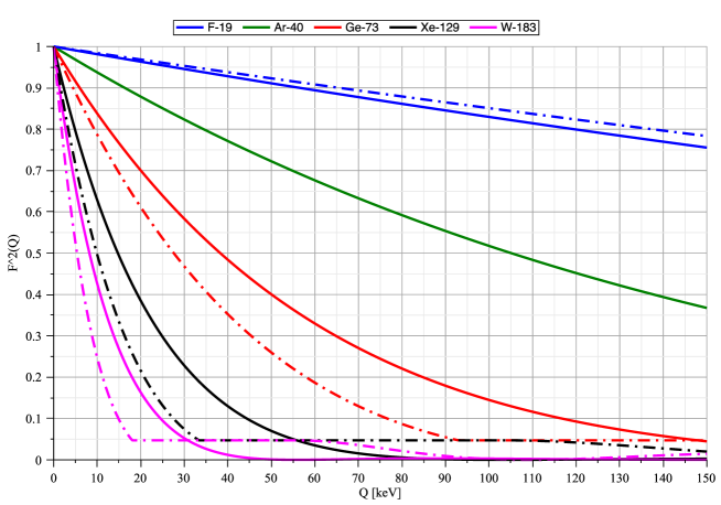
Figure 8: Nuclear form factors of the ${}^{19}{\rm F}$ (blue), the ${}^{40}{\rm Ar}$ (green), the ${}^{73}{\rm Ge}$ (red), the ${}^{129}{\rm Xe}$ (black), and the ${}^{183}{\rm W}$ (magenta) nuclei as functions of the recoil energy. The solid and dash–dotted curves indicate the form factors corresponding to the SI and SD cross sections, $F_{\rm SI}^{2}(Q)$ and $F_{\rm SD}^{2}(Q)$, given in Eqs. (32) and (33), respectively.

In Fig. 8, we show the recoil–energy dependences of the nuclear form factors corresponding to the SI (solid) and SD (dash–dotted) cross sections, $F_{\rm SI}^{2}(Q)$ and $F_{\rm SD}^{2}(Q)$, given in Eqs. (32) and (33), respectively. Five frequently used target nuclei have been considered: ${}^{19}{\rm F}$ (blue), ${}^{40}{\rm Ar}$ (green), ${}^{73}{\rm Ge}$ (red), ${}^{129}{\rm Xe}$ (black), and ${}^{183}{\rm W}$ (magenta). The sharply enlarged nuclear form factor suppression in the validation criterion (25) or (31) with the increased mass of the target nucleus can be seen clearly.

In Refs. [21] and [22], we will discuss in detail the effects of the cross section (nuclear form factor) suppression on the angular distributions of the nuclear recoil direction (flux)/energy as well as on the 3-D effective velocity distribution of incident halo WIMPs separately.

4.2.3 WIMP–mass dependence of the recoil energy

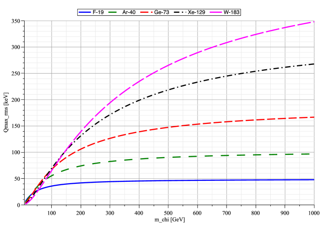
Figure 9: The WIMP–mass dependence of the maximum of the recoil energy, $Q_{\rm max,rms}$, given by Eq. (37). Five frequently used target nuclei: ${}^{19}{\rm F}$ (solid blue), ${}^{40}{\rm Ar}$ (rare–dashed green), ${}^{73}{\rm Ge}$ (dashed red), ${}^{129}{\rm Xe}$ (dash–dotted black), and ${}^{183}{\rm W}$ (long–dashed magenta) have been considered.

For readers’ reference, in Fig. 9 we show the WIMP–mass dependence of the maximum (prefactor) of the recoil energy $Q$ given by Eq. (19) with the monotonic root–mean–square velocity of incident halo WIMPs:

$$Q_{\rm max,rms}=\left(\frac{2m_{\rm r,N}^{2}}{m_{\rm N}}\right)v_{\rm rms,Lab}^{2}~{}\!,$$ (37)

for five frequently used target nuclei: ${}^{19}{\rm F}$ (solid blue), ${}^{40}{\rm Ar}$ (rare–dashed green), ${}^{73}{\rm Ge}$ (dashed red), ${}^{129}{\rm Xe}$ (dash–dotted black), and ${}^{183}{\rm W}$ (long–dashed magenta). Here, although it would be somehow inconsistent with our observations presented in Ref. [19] (see detailed discussions therein), we use the shifted Maxwellian velocity distribution function [2]:

$$f_{1,{\rm sh}}(v_{\chi,{\rm Lab}})=\frac{1}{\sqrt{\pi}}\left(\frac{v_{\chi,{\rm Lab}}}{v_{0}v_{\rm e}}\right)\bigg{[}e^{-(v_{\chi,{\rm Lab}}-v_{\rm e})^{2}/v_{0}^{2}}-e^{-(v_{\chi,{\rm Lab}}+v_{\rm e})^{2}/v_{0}^{2}}\bigg{]}~{}\!,$$ (38)

as a useful approximation to the radial component (magnitude) of the 3-D WIMP velocity distribution in the Equatorial/laboratory coordinate systems, where $v_{\rm e}$ is the time–dependent Earth’s velocity in the Galactic frame [24, 2]:

$$v_{\rm e}(t)=v_{0}\left[1.05+0.07\cos\left(\frac{2\pi(t-t_{\rm p})}{1~{}{\rm yr}}\right)\right]~{}\!,$$ (39)

with $t_{\rm p}\simeq$ June 2nd, the date on which the Earth’s orbital speed is maximal. Then the root–mean–square velocity of incident halo WIMPs can be obtained as

$$v_{\rm rms,Lab}^{2} = \left<{v_{\chi,{\rm Lab}}^{2}}\right>_{{\rm sh}}=\int_{0}^{\infty}v_{\chi,{\rm Lab}}^{2}~{}\!f_{1,{\rm sh}}(v_{\chi,{\rm Lab}})~{}\!dv_{\chi,{\rm Lab}}=\left(\frac{3}{2}\right)v_{0}^{2}+v_{\rm e}^{2}$$ (40)

$$\simeq (355~{}{\rm km/s})^{2}~{}\!.$$

In the last line, the time dependence of $v_{\rm e}(t)$ has been ignored and $v_{\rm e}=1.05~{}\!v_{0}$ is used.

In Refs. [21] and [22], we will demonstrate the WIMP–mass dependence of the cross section (nuclear form factor) suppression on the angular recoil–direction/energy distributions as well as on the 3-D WIMP effective velocity distribution separately.

5 Summary

As the preparation of our development of data analysis procedures for using and/or combining 3-dimensional information offered by directional direct Dark Matter detection experiments in the future, we finally achieved our double–Monte Carlo scattering–by–scattering simulation of 3-dimensional elastic WIMP–nucleus scattering process, which can provide 3-D information (the magnitude, the direction, and the incoming/scattering time) of each incident halo WIMP as well as the experimentally measurable recoil direction and recoil energy of the WIMP–scattered target nucleus event by event in different celestial coordinate systems.

In this paper, we described at first the overall workflow of our simulation procedure. After the summary of the MC generation process of the 3-D velocity information of Galactic WIMPs and the transformations of the 3-D (velocity) information between different celestial coordinate systems, we introduced the incoming–WIMP coordinate system for describing the 3-D WIMP–nucleus scattering process and derived the validation criterion in our MC generation of the 3-D recoil information of scattered target nuclei, which is basically according to the cross section (nuclear form factor) suppression on the recoil–angle–dependent recoil energy.

Currently, several approximations about the Earth’s orbital motion in the Solar system and the observation periods/daily shifts have been used in our simulation package. First, the Earth’s orbit around the Sun is perfectly circular on the Ecliptic plane and the orbital speed is thus a constant. Second, the date of the vernal equinox is exactly fixed at the end of the May 20th (the 79th day) of a 365-day year and the few extra hours in an actual Solar year have been neglected. Nevertheless, considering the very low WIMP scattering event rate and thus maximal a few (tens) of total WIMP events observed in at least a few tens (or even hundreds) of days (an optimistic overall event rate of $\>\raisebox{-3.01385pt}{$\stackrel{{\scriptstyle\textstyle<}}{{\sim}}$}\>~{}\!{\cal O}(1)$ event/day) for the first–phase analyses, these approximations should be acceptable.

Hopefully, this (and more works fulfilled in the future) could help our colleagues to develop analysis methods for understanding the astrophysical and particle properties of Galactic WIMPs as well as the structure of Dark Matter halo by using directional direct detection data.

Acknowledgments

The author appreciates N. Bozorgnia and P. Gondolo for useful discussions about the transformations between the celestial coordinate systems. The author would like to thank the friendly hospitality of the Gran Sasso Science Institute as well as the pleasant atmosphere of the W101 Ward and the Cancer Center of the Kaohsiung Veterans General Hospital, where part of this work was completed. This work was strongly encouraged by the “Researchers working on e.g. exploring the Universe or landing on the Moon should not stay here but go abroad.” speech.

Appendix A Definitions of and transformations between our coordinate systems

In this section, we review briefly our definitions of the laboratory–independent (Galactic, Ecliptic, Equatorial, and Earth) coordinate systems as well as the laboratory–dependent (horizontal and laboratory) coordinate systems used in our simulation package. We also summarize the matrices needed for the transformations (of the 3-D velocity) between these coordinate systems.

Discussions about our coordinate systems as well as the detailed derivations of the transformation matrices between them can be found in Ref. [19].

A.1 Laboratory–independent coordinate systems

We consider the Galactic, the Ecliptic, and the Equatorial coordinate systems at first.

A.1.1 Definitions

In Fig. A1, we show the definitions of and the relative orientations between the (black) Galactic, the (red) Ecliptic, and the (blue) Equatorial coordinate systems (on the date of the vernal equinox).

Figure A1: The definitions of and the relative orientations between the (black) Galactic, the (red) Ecliptic, and the (blue) Equatorial coordinate systems (on the date of the vernal equinox). While the magenta circular band indicates an approximate path of the orbital motion of the Solar system in the Galaxy and the blue circular band the Earth’s orbit around the Sun, the additional (golden) arrows indicate the direction of the movement of the Solar system around the Galactic center. See the text for the detailed descriptions.

Firstly, the origin of the Galactic coordinate system is at the (approximate) Galactic Center (GC). The primary direction (the ${\bf X}_{\rm G}$–axis) points from the Solar center to GC and the ${\bf Z}_{\rm G}$–axis to the Galactic North Pole (GNP). Then the right–handed convention is used for defining the ${\bf Y}_{\rm G}$–axis and the fundamental (${\bf X}_{\rm G}-{\bf Y}_{\rm G}$) plane is the approximate Galactic plane [31].

Meanwhile, the origins of the Ecliptic and the Equatorial coordinate systems are at the center of the Sun and that of the Earth, respectively. The common primary direction (the ${\bf X}_{\rm S}$/${\bf X}_{\rm Eq}$–axis) is the direction pointing from the Solar center to that of the Earth at 12 midnight (the end) of the date of the vernal equinox, the ${\bf Z}_{\rm S}$– and the ${\bf Z}_{\rm Eq}$–axes are perpendicular to the (yellow) Ecliptic and the (blue) Equatorial planes, respectively, and their ${\bf Y}_{\rm S}$– and ${\bf Y}_{\rm Eq}$–axes are then defined as usual by the right–handed convention.

Additionally, in Fig. A1, we also draw two (golden) arrows to indicate the direction of the movement of the Solar system towards the CYGNUS constellation. Note that the moving direction of the Solar system is not parallel to, but only approximately along the ${\bf Y}_{\rm G}$–axis, (with an included angle of 8.87^∘ = 35.48^m), nor on the (approximate) Galactic plane (0.60^∘ above).

Note also that the Ecliptic coordinate system only moves approximately linearly with the Solar Galactic orbital velocity $v_{\rm\odot,G}=|{\bf v}_{\rm\odot,G}|\simeq 220$ km/s and the tiny Galactic orbital rotation of the Solar system is considered to be imperceptible, whereas the Equatorial coordinate system moves orbitally around (and also linearly with) the Sun, but doesn’t rotate. These mean that the axes of the Galactic, the Ecliptic, and the Equatorial coordinate systems defined in our simulation package are all fixed (see Table A1 for the summary of the styles of the movements and the rotations of different celestial coordinate systems).

A.1.2 Transformation matrices

At first, by definition, the transformation matrix from the Ecliptic coordinate system to the Equatorial coordinate system can be given directly as

$${\bf M}_{\rm S\to Eq}=\left[\begin{array}[]{c c c}1{}&~{}0{}&~{}0\\ 0{}&~{}\cos(\psi_{\oplus}){}&~{}\sin(\psi_{\oplus})\\ 0{}&~{}-\sin(\psi_{\oplus}){}&~{}\cos(\psi_{\oplus})\\ \end{array}\right]=\left[\begin{array}[]{c c c}1{}&~{}0{}&~{}0\\ 0{}&~{}0.91775{}&~{}0.39715\\ 0{}&~{}-0.39715{}&~{}0.91775\\ \end{array}\right]~{}\!,$$ (A7a)

and, conversely,

$${\bf M}_{\rm Eq\to S}=\left[\begin{array}[]{c c c}1{}&~{}0{}&~{}0\\ 0{}&~{}\cos(\psi_{\oplus}){}&~{}-\sin(\psi_{\oplus})\\ 0{}&~{}\sin(\psi_{\oplus}){}&~{}\cos(\psi_{\oplus})\\ \end{array}\right]=\left[\begin{array}[]{c c c}1{}&~{}0{}&~{}0\\ 0{}&~{}0.91775{}&~{}-0.39715\\ 0{}&~{}0.39715{}&~{}0.91775\\ \end{array}\right]~{}\!,$$ (A7b)

where $\psi_{\oplus}=23.4^{\circ}$ is the Earth’s obliquity.

On the other hand, the directions of the Galactic Center and the Galactic North Pole in the Equatorial coordinate system can be expressed by

$${\bf X}_{\rm G,Eq} = \left[\begin{array}[]{c c c}\cos(\theta_{\rm GC,Eq})\cos(\phi_{\rm GC,Eq}){}&~{}\cos(\theta_{\rm GC,Eq})\sin(\phi_{\rm GC,Eq}){}&~{}\sin(\theta_{\rm GC,Eq})\\ \end{array}\right]_{\rm Eq}$$ (A9a)

$$\cong \left[\begin{array}[]{c c c}0.05495{}&~{}0.87340{}&~{}-0.48389\\ \end{array}\right]_{\rm Eq}~{}\!,$$ (A11a)

and

$${\bf Z}_{\rm G,Eq} = \left[\begin{array}[]{c c c}\cos(\theta_{\rm GNP,Eq})\cos(\phi_{\rm GNP,Eq}){}&~{}\cos(\theta_{\rm GNP,Eq})\sin(\phi_{\rm GNP,Eq}){}&~{}\sin(\theta_{\rm GNP,Eq})\\ \end{array}\right]_{\rm Eq}$$ (A12b)

$$\cong \left[\begin{array}[]{c c c}0.86769{}&~{}0.19793{}&~{}0.45601\\ \end{array}\right]_{\rm Eq}~{}\!,$$ (A14b)

respectively, where we have adopted the values provided by Ref. [31]

$$\phi_{\rm GC,Eq}=5^{\rm h}45.6^{\rm m}=86.40^{\circ}~{}\!,~{}~{}~{}~{}~{}~{}~{}~{}~{}~{}~{}~{}~{}~{}~{}~{}~{}~{}~{}~{}\theta_{\rm GC,Eq}=-28.94^{\circ}~{}\!,$$ (A15)

and

$$\phi_{\rm GNP,Eq}=51.4^{\rm m}=12.85^{\circ}~{}\!,~{}~{}~{}~{}~{}~{}~{}~{}~{}~{}~{}~{}~{}~{}~{}~{}~{}~{}~{}~{}~{}\theta_{\rm GNP,Eq}=27.13^{\circ}~{}\!,$$ (A16)

as the right ascensions and the declinations of GC and GNP in the Equatorial coordinate system, respectively.

Then, by combining Eqs. (A11a) and (A14b), the ${\bf Y}_{\rm G}$–axis of the Galactic coordinate system in the Equatorial coordinate system can be calculated by

$${\bf Y}_{\rm G,Eq} = {\bf Z}_{\rm G,Eq}\times{\bf X}_{\rm G,Eq}$$ (A17c)

$$= \footnotesize\left[\begin{array}[]{c}\cos(\theta_{\rm GNP,Eq})\sin(\phi_{\rm GNP,Eq})\sin(\theta_{\rm GC,Eq})-\sin(\theta_{\rm GNP,Eq})\cos(\theta_{\rm GC,Eq})\sin(\phi_{\rm GC,Eq})\\ \sin(\theta_{\rm GNP,Eq})\cos(\theta_{\rm GC,Eq})\cos(\phi_{\rm GC,Eq})-\cos(\theta_{\rm GNP,Eq})\cos(\phi_{\rm GNP,Eq})\sin(\theta_{\rm GC,Eq})\\ \cos(\theta_{\rm GNP,Eq})\cos(\theta_{\rm GC,Eq})\Big{[}\cos(\phi_{\rm GNP,Eq})\sin(\phi_{\rm GC,Eq})-\sin(\phi_{\rm GNP,Eq})\cos(\phi_{\rm GC,Eq})\Big{]}\\ \end{array}\right]_{\rm Eq}^{\rm T}$$

$$\cong \left[\begin{array}[]{c c c}-0.49406{}&~{}0.44492{}&~{}0.74696\\ \end{array}\right]_{\rm Eq}~{}\!.$$ (A19c)

Hence, the transformation matrices between the Equatorial and the Galactic coordinate systems can be given by

$${\bf M}_{\rm Eq\to G}=\left[\begin{array}[]{c}{\bf X}_{\rm G,Eq}\\ {\bf Y}_{\rm G,Eq}\\ {\bf Z}_{\rm G,Eq}\\ \end{array}\right]=\left[\begin{array}[]{c c c}0.05495{}&~{}0.87340{}&~{}-0.48389\\ -0.49406{}&~{}0.44492{}&~{}0.74696\\ 0.86769{}&~{}0.19793{}&~{}0.45601\\ \end{array}\right]~{}\!,$$ (A22a)

and, conversely,

$${\bf M}_{\rm G\to Eq}=\left[\begin{array}[]{c c c}0.05495{}&~{}-0.49406{}&~{}0.86769\\ 0.87340{}&~{}0.44492{}&~{}0.19793\\ -0.48389{}&~{}0.74696{}&~{}0.45601\\ \end{array}\right]~{}\!.$$ (A22b)

Moreover, by combining the transformation matrices between the Equatorial and the Ecliptic coordinate systems in Eqs. (A7b) and (A7a), the transformations between the Ecliptic and the Galactic coordinate systems can be obtained by

$${\bf M}_{\rm G\to S}={\bf M}_{\rm Eq\to S}{\bf M}_{\rm G\to Eq}=\left[\begin{array}[]{c c c}0.05495{}&~{}-0.49406{}&~{}0.86769\\ 0.99374{}&~{}0.11168{}&~{}0.00055\\ -0.09723{}&~{}0.86223{}&~{}0.49711\\ \end{array}\right]~{}\!,$$ (A23a)

and

$${\bf M}_{\rm S\to G}={\bf M}_{\rm Eq\to G}{\bf M}_{\rm S\to Eq}=\left[\begin{array}[]{c c c}0.05495{}&~{}0.99374{}&~{}-0.09723\\ -0.49406{}&~{}0.11168{}&~{}0.86223\\ 0.86769{}&~{}0.00055{}&~{}0.49711\\ \end{array}\right]~{}\!.$$ (A23b)

A.1.3 Direction of the Galactic movement of the Solar system

For readers’ reference, the direction (the right ascension and the declination) of the Galactic movement of the Solar system towards the CYGNUS constellation in the Galactic, the Ecliptic, and the Equatorial coordinate systems are summarized here:

$$\phi_{\rm Cyg,G}=5.41^{\rm h}=81.22^{\circ}~{}\!,~{}~{}~{}~{}~{}~{}~{}~{}~{}~{}~{}~{}~{}~{}~{}~{}~{}~{}~{}~{}~{}~{}~{}\!\theta_{\rm Cyg,G}=0.60^{\circ}~{}\!,$$ (A24)

$$\phi_{\rm Cyg,S}=10.06^{\rm h}=150.90^{\circ}~{}\!,~{}~{}~{}~{}~{}~{}~{}~{}~{}~{}~{}~{}~{}~{}~{}~{}~{}~{}~{}~{}\theta_{\rm Cyg,S}=57.40^{\circ}~{}\!,$$ (A25)

and [32]

$$\phi_{\rm Cyg,Eq}=8.62^{\rm h}=129.30^{\circ}~{}\!,~{}~{}~{}~{}~{}~{}~{}~{}~{}~{}~{}~{}~{}~{}~{}~{}~{}~{}~{}~{}\>\!\theta_{\rm Cyg,Eq}=42^{\circ}~{}\!.$$ (A26)

Detailed derivations can be found in Ref. [19].

A.2 Earth coordinate system

As the connection of the Equatorial and Ecliptic coordinate systems to the horizontal and laboratory coordinate systems [32], we defined the Earth coordinate system in our simulation package.

A.2.1 Definition

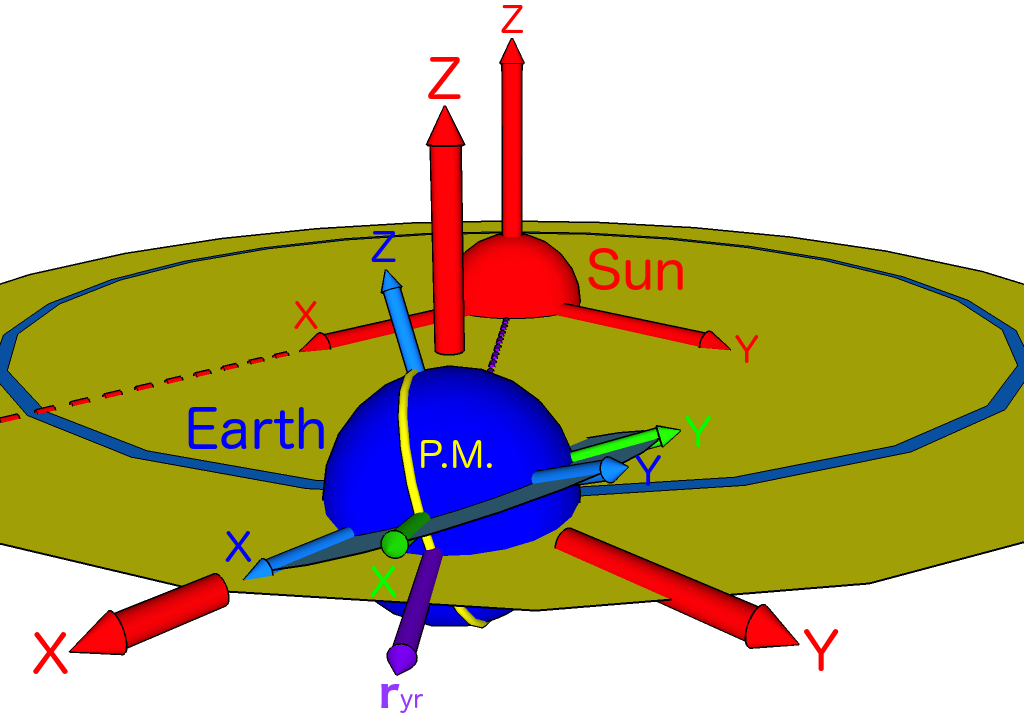
Figure A2: The definition of the (light–green) Earth coordinate system at 12 midnight (the beginning) (i.e., when the (yellow) Prime Meridian (the longitude 0^∘) passes the purple arrow pointing from the Solar center to that of the Earth) of each single “Solar” day. The (red) Ecliptic and the (blue) Equatorial coordinate systems as well as the (blue) Earth’s orbit around the Sun are also given here. See the text for the detailed description.

As shown in Fig. A2, we define the Earth coordinate system as follows: while the origin is also located at the Earth’s center and the ${\bf Z}_{\rm E}$–axis is still the Earth’s north polar axis, the primary direction (the ${\bf X}_{\rm E}$–axis) points now from the Earth’s center to the Prime Meridian (the longitude 0^∘) at 12 midnight (the beginning) (i.e., when the Prime Meridian passes the direction pointing from the Solar center to that of the Earth) of each single “Solar” day. The fundamental (${\bf X}_{\rm E}-{\bf Y}_{\rm E}$) plane is again the Equatorial plane and the right–hand convention is used to define the ${\bf Y}_{\rm E}$–axis.

Note that, for each single (Solar) day, the Earth coordinate system is fixed with the direction of the Prime Meridian at (UTC) 12 midnight, but rotates with the Earth during the its orbital motion around the Sun. This means that our Earth coordinate system changes daily and discretely (see Table A1).

A.2.2 Transformation matrices

Following the calculations done by A. Bandyopadhyay and D. Majumdar in Ref. [32], the transformation matrices between the Equatorial and the Earth coordinate systems can be expressed by [19]

$${\bf M}_{\rm Eq\to E}(t)=\left[\begin{array}[]{c c c}\gamma(t)\cos(\psi_{\rm yr}(t)){}&~{}\gamma(t)\sin(\psi_{\rm yr}(t))\cos(\psi_{\oplus}){}&~{}0\\ -\gamma(t)\sin(\psi_{\rm yr}(t))\cos(\psi_{\oplus}){}&~{}\gamma(t)\cos(\psi_{\rm yr}(t)){}&~{}0\\ 0{}&~{}0{}&~{}1\\ \end{array}\right]~{}\!,$$ (A27a)

and, conversely,

$${\bf M}_{\rm E\to Eq}(t)=\left[\begin{array}[]{c c c}\gamma(t)\cos(\psi_{\rm yr}(t)){}&~{}-\gamma(t)\sin(\psi_{\rm yr}(t))\cos(\psi_{\oplus}){}&~{}0\\ \gamma(t)\sin(\psi_{\rm yr}(t))\cos(\psi_{\oplus}){}&~{}\gamma(t)\cos(\psi_{\rm yr}(t)){}&~{}0\\ 0{}&~{}0{}&~{}1\\ \end{array}\right]~{}\!,$$ (A27b)

where we define

$$\gamma(t)\equiv\frac{1}{\sqrt{\cos^{2}(\psi_{\rm yr}(t))+\sin^{2}(\psi_{\rm yr}(t))\cos^{2}(\psi_{\oplus})}}~{}\!.$$ (A28)

A.3 Laboratory–dependent coordinate systems

Now we come to the horizontal and the laboratory coordinate systems.

A.3.1 Definitions

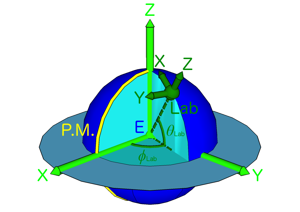
(a)

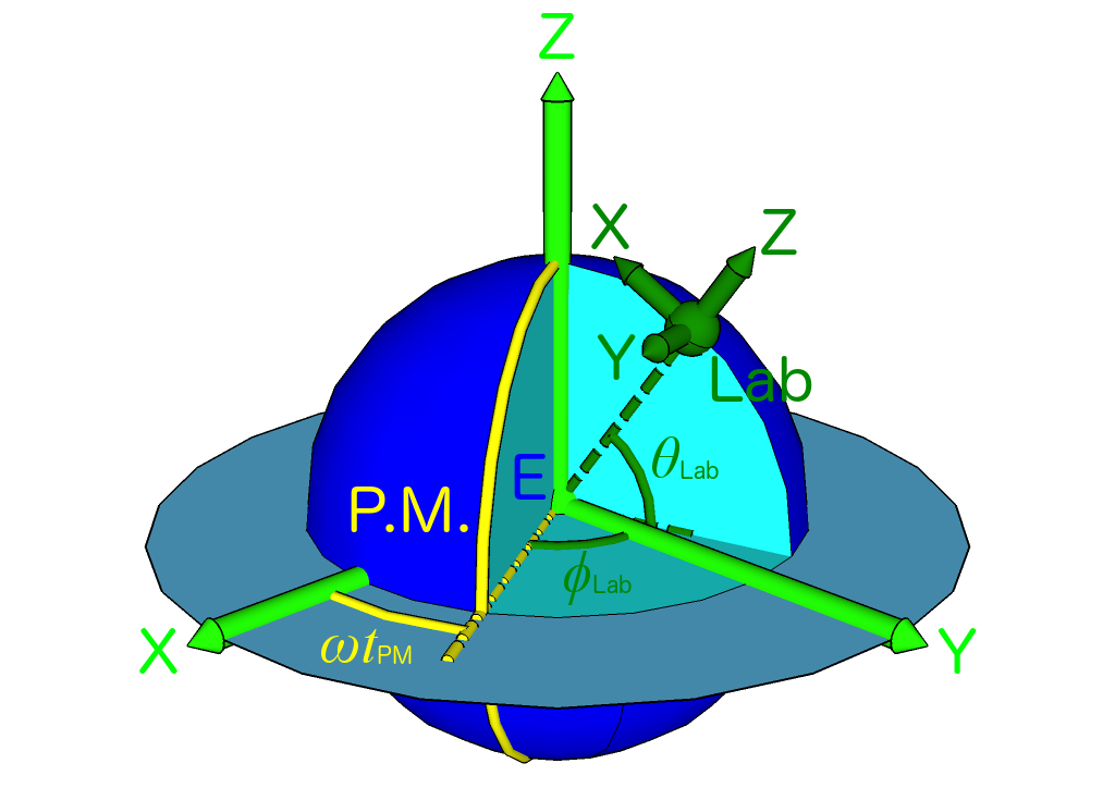
(b)

Figure A3: The definitions of the (dark–green) horizontal (a) and laboratory (b) coordinate systems. $\phi_{\rm Lab}$ and $\theta_{\rm Lab}$ indicate the longitude and the latitude of the location of the laboratory of interest, respectively. $\omega t_{\rm PM}$ indicates the rotation angle of the (yellow) Prime Meridian from (UTC) 12 midnight (the beginning) of each single Solar day. As a reference, our (light–green) Earth coordinate system is also sketched here. See the text for the detailed descriptions.

In Fig. A3 we sketch the definitions of the (dark–green) horizontal (a) and laboratory (b) coordinate systems, respectively. Our (light–green) Earth coordinate system is also sketched here as a reference.

At first, the origin of the horizontal coordinate system is chosen as the location of the laboratory of interest at (UTC) 12 midnight (the beginning) of each single Solar day with $\phi_{\rm Lab}$ and $\theta_{\rm Lab}$ indicating the longitude and the latitude of the laboratory location, respectively. The primary direction (the ${\bf X}_{\rm H}$–axis) and the ${\bf Z}_{\rm H}$–axis point towards north and the zenith, respectively. Then, as usual, the right–handed convention is used for defining the ${\bf Y}_{\rm H}$–axis. Note that, as the Earth coordinate system, for each single (Solar) day, our horizontal coordinate system is fixed with the direction of the Prime Meridian at (UTC) 12 midnight and thus changes daily and discretely.

Moreover, we consider also the instantaneous (UTC) incoming/scattering time of each recorded WIMP event and define our laboratory coordinate system. It is basically the same as the horizontal coordinate system, but rotates with the considered laboratory around the Earth’s north polar (${\bf Z}_{\rm Eq}/{\bf Z}_{\rm E}$–axis) by an angle of $\omega t_{\rm PM}$, where

$$\omega\equiv\frac{2\pi}{1~{}{\rm day}}~{}\!,$$ (A29)

and $t_{\rm PM}$ indicates the fractional part of the UTC incoming/scattering time $t$ of each recorded WIMP event in unit of day. Note that our laboratory coordinate system changes (rotates around the Earth’s north polar axis) event by event (see Table A1).

A.3.2 Transformation matrices

At first, the transformation matrices between the Earth and the horizontal coordinate systems can be given by [19]

$${\bf M}_{\rm E\to H}(\phi_{\rm Lab},\theta_{\rm Lab})={\small\left[\begin{array}[]{c c c}-\cos(\phi_{\rm Lab})\sin(\theta_{\rm Lab}){}&~{}-\sin(\phi_{\rm Lab})\sin(\theta_{\rm Lab}){}&~{}\cos(\theta_{\rm Lab})\\ \sin(\phi_{\rm Lab}){}&~{}-\cos(\phi_{\rm Lab}){}&~{}0\\ \cos(\phi_{\rm Lab})\cos(\theta_{\rm Lab}){}&~{}\sin(\phi_{\rm Lab})\cos(\theta_{\rm Lab}){}&~{}\sin(\theta_{\rm Lab})\\ \end{array}\right]}~{}\!,$$ (A30a)

and then, conversely, we have

$${\bf M}_{\rm H\to E}(\phi_{\rm Lab},\theta_{\rm Lab})={\small\left[\begin{array}[]{c c c}-\cos(\phi_{\rm Lab})\sin(\theta_{\rm Lab}){}&~{}\sin(\phi_{\rm Lab}){}&~{}\cos(\phi_{\rm Lab})\cos(\theta_{\rm Lab})\\ -\sin(\phi_{\rm Lab})\sin(\theta_{\rm Lab}){}&~{}-\cos(\phi_{\rm Lab}){}&~{}\sin(\phi_{\rm Lab})\cos(\theta_{\rm Lab})\\ \cos(\theta_{\rm Lab}){}&~{}0{}&~{}\sin(\theta_{\rm Lab})\\ \end{array}\right]}~{}\!.$$ (A30b)

Remind that, since, by our definitions, both of the Earth and the horizontal coordinate systems are fixed with the direction of the Prime Meridian at (UTC) 12 midnight of each single Solar day, the transformations between them depend only on the location (the longitude and the latitude) of the considered laboratory.

Similarly the transformation matrices between the Earth and the laboratory coordinate systems can be obtained directly as

$${\bf M}_{\rm E\to Lab}(t,\phi_{\rm Lab},\theta_{\rm Lab})$$ (A34a)

$$= {\footnotesize\left[\begin{array}[]{c c c}-\cos\left(\phi_{\rm Lab}+\omega t_{\rm PM}\right)\sin(\theta_{\rm Lab}){}&~{}-\sin\left(\phi_{\rm Lab}+\omega t_{\rm PM}\right)\sin(\theta_{\rm Lab}){}&~{}\cos(\theta_{\rm Lab})\\ \sin\left(\phi_{\rm Lab}+\omega t_{\rm PM}\right){}&~{}-\cos\left(\phi_{\rm Lab}+\omega t_{\rm PM}\right){}&~{}0\\ \cos\left(\phi_{\rm Lab}+\omega t_{\rm PM}\right)\cos(\theta_{\rm Lab}){}&~{}\sin\left(\phi_{\rm Lab}+\omega t_{\rm PM}\right)\cos(\theta_{\rm Lab}){}&~{}\sin(\theta_{\rm Lab})\\ \end{array}\right]}~{}\!,$$

and

$${\bf M}_{\rm Lab\to E}(t,\phi_{\rm Lab},\theta_{\rm Lab})$$ (A37b)

$$= {\footnotesize\left[\begin{array}[]{c c c}-\cos\left(\phi_{\rm Lab}+\omega t_{\rm PM}\right)\sin(\theta_{\rm Lab}){}&~{}\sin\left(\phi_{\rm Lab}+\omega t_{\rm PM}\right){}&~{}\cos\left(\phi_{\rm Lab}+\omega t_{\rm PM}\right)\cos(\theta_{\rm Lab})\\ -\sin\left(\phi_{\rm Lab}+\omega t_{\rm PM}\right)\sin(\theta_{\rm Lab}){}&~{}-\cos\left(\phi_{\rm Lab}+\omega t_{\rm PM}\right){}&~{}\sin\left(\phi_{\rm Lab}+\omega t_{\rm PM}\right)\cos(\theta_{\rm Lab})\\ \cos(\theta_{\rm Lab}){}&~{}0{}&~{}\sin(\theta_{\rm Lab})\\ \end{array}\right]}~{}\!.$$

Then, by combining Eqs. (A30b) and (A37b) with Eqs. (A34a) and (A30a), the transformation matrices between the horizontal and the laboratory coordinate systems can be expressed as

$${\bf M}_{\rm H\to Lab}(t,\phi_{\rm Lab},\theta_{\rm Lab})$$ (A41a)

$$= {\bf M}_{\rm E\to Lab}(t,\phi_{\rm Lab},\theta_{\rm Lab})~{}\!{\bf M}_{\rm H\to E}(\phi_{\rm Lab},\theta_{\rm Lab})$$

$$= {\scriptsize\left[\begin{array}[]{c c c}\cos(\omega t_{\rm PM})\sin^{2}(\theta_{\rm Lab})+\cos^{2}(\theta_{\rm Lab}){}&~{}\sin(\omega t_{\rm PM})\sin(\theta_{\rm Lab}){}&~{}\big{[}1-\cos(\omega t_{\rm PM})\big{]}\sin(\theta_{\rm Lab})\cos(\theta_{\rm Lab})\\ -\sin(\omega t_{\rm PM})\sin(\theta_{\rm Lab}){}&~{}\cos(\omega t_{\rm PM}){}&~{}\sin(\omega t_{\rm PM})\cos(\theta_{\rm Lab})\\ \big{[}1-\cos(\omega t_{\rm PM})\big{]}\sin(\theta_{\rm Lab})\cos(\theta_{\rm Lab}){}&~{}-\sin(\omega t_{\rm PM})\cos(\theta_{\rm Lab}){}&~{}\cos(\omega t_{\rm PM})\cos^{2}(\theta_{\rm Lab})+\sin^{2}(\theta_{\rm Lab})\\ \end{array}\right]},$$

and

$${\bf M}_{\rm Lab\to H}(t,\phi_{\rm Lab},\theta_{\rm Lab})$$ (A44b)

$$= {\bf M}_{\rm E\to H}(\phi_{\rm Lab},\theta_{\rm Lab})~{}\!{\bf M}_{\rm Lab\to E}(t,\phi_{\rm Lab},\theta_{\rm Lab})$$

$$= {\scriptsize\left[\begin{array}[]{c c c}\cos(\omega t_{\rm PM})\sin^{2}(\theta_{\rm Lab})+\cos^{2}(\theta_{\rm Lab}){}&~{}-\sin(\omega t_{\rm PM})\sin(\theta_{\rm Lab}){}&~{}\big{[}1-\cos(\omega t_{\rm PM})\big{]}\sin(\theta_{\rm Lab})\cos(\theta_{\rm Lab})\\ \sin(\omega t_{\rm PM})\sin(\theta_{\rm Lab}){}&~{}\cos(\omega t_{\rm PM}){}&~{}-\sin(\omega t_{\rm PM})\cos(\theta_{\rm Lab})\\ \big{[}1-\cos(\omega t_{\rm PM})\big{]}\sin(\theta_{\rm Lab})\cos(\theta_{\rm Lab}){}&~{}\sin(\omega t_{\rm PM})\cos(\theta_{\rm Lab}){}&~{}\cos(\omega t_{\rm PM})\cos^{2}(\theta_{\rm Lab})+\sin^{2}(\theta_{\rm Lab})\\ \end{array}\right]}.$$

Note that, while the transformations between the Earth and the laboratory coordinate systems in Eqs. (A34a) to (A37b) depend on both of the laboratory location and the incoming/scattering time of each WIMP event (recorded in the considered laboratory), those between the horizontal and the laboratory coordinate systems are longitude ($\phi_{\rm Lab}$) independent and depend only on the latitude of the laboratory location $\theta_{\rm Lab}$ and the incoming/scattering time $t$.

Coordinate system	Movement	Rotation	Style
Galactic	$\times$	$\times^{\dagger}$	Fixed
Ecliptic	$\surd$	$\times$	Orbital $\to$ approximately linear
Equatorial	$\surd$	$\times$	Linear + orbital $\to$ spiral
Earth	$\times^{\ddagger}$	$\surd$	Daily and discrete
Horizontal	$\times^{\ddagger}$	$\surd$	Daily and discrete
Laboratory	$\times^{\ddagger}$	$\surd$	Instantaneous and continuous

Table A1: The summary of the styles of the movements and the rotations of all six celestial coordinate systems defined in our simulation package.
^†: The tiny angle swept by the connection between the Solar and the Galactic centers during the orbital motion of the Solar system in the Galaxy is ignored in our package.
^‡: Fixed on the Earth and combined additionally with the “linear + orbital $\to$ spiral” movement of the Equatorial coordinate system.

A.4 Incoming–WIMP coordinate system

For our Monte Carlo simulation of 3-D elastic WIMP–nucleus scattering events, we have introduced the “incoming–WIMP” coordinate system defined in Sec. 4.1.

A.4.1 Transformation matrices

Similar to the transformations between the horizontal and the Earth coordinate systems, the transformation from the incoming–WIMP coordinate system to the laboratory coordinate system can be done by rotating at first $\pi/2-\theta_{\rm\chi,Lab}$ around the ${\bf Y}_{\chi_{\rm in}}$–axis and then $\pi-\phi_{\rm\chi,Lab}$ around the ${\bf Z}_{\chi_{\rm in}}$–axis (see Fig. 6) and can thus be given by

$${\bf M}_{\rm\chi_{in}\to Lab}(\phi_{\rm\chi,Lab},\theta_{\rm\chi,Lab})$$ (A48a)

$$= \left[\begin{array}[]{c c c}-\cos(\phi_{\rm\chi,Lab})\sin(\theta_{\rm\chi,Lab}){}&~{}\sin(\phi_{\rm\chi,Lab}){}&~{}\cos(\phi_{\rm\chi,Lab})\cos(\theta_{\rm\chi,Lab})\\ -\sin(\phi_{\rm\chi,Lab})\sin(\theta_{\rm\chi,Lab}){}&~{}-\cos(\phi_{\rm\chi,Lab}){}&~{}\sin(\phi_{\rm\chi,Lab})\cos(\theta_{\rm\chi,Lab})\\ \cos(\theta_{\rm\chi,Lab}){}&~{}0{}&~{}\sin(\theta_{\rm\chi,Lab})\\ \end{array}\right]~{}\!.$$

Conversely, we also have

$${\bf M}_{\rm Lab\to\chi_{in}}(\phi_{\rm\chi,Lab},\theta_{\rm\chi,Lab})$$ (A51b)

$$= \left[\begin{array}[]{c c c}-\cos(\phi_{\rm\chi,Lab})\sin(\theta_{\rm\chi,Lab}){}&~{}-\sin(\phi_{\rm\chi,Lab})\sin(\theta_{\rm\chi,Lab}){}&~{}\cos(\theta_{\rm\chi,Lab})\\ \sin(\phi_{\rm\chi,Lab}){}&~{}-\cos(\phi_{\rm\chi,Lab}){}&~{}0\\ \cos(\phi_{\rm\chi,Lab})\cos(\theta_{\rm\chi,Lab}){}&~{}\sin(\phi_{\rm\chi,Lab})\cos(\theta_{\rm\chi,Lab}){}&~{}\sin(\theta_{\rm\chi,Lab})\\ \end{array}\right]~{}\!.$$

References

• [1]
• [2] G. Jungman, M. Kamionkowski and K. Griest, “Supersymmetric Dark Matter”, Phys. Rep. 267, 195–373 (1996), arXiv:hep-ph/9506380.
• [3] R. J. Gaitskell, “Direct Detection of Dark Matter”, Ann. Rev. Nucl. Part. Sci. 54, 315–359 (2004).
• [4] L. Baudis, “Direct Dark Matter Detection: the Next Decade”, Issue on “The Next Decade in Dark Matter and Dark Energy”, Phys. Dark Univ. 1, 94–108 (2012), arXiv:1211.7222 [astro-ph.IM].
• [5] L. Baudis, “Dark Matter Searches”, Annalen Phys. 528, 74–83 (2016), arXiv:1509.00869 [astro-ph.CO].
• [6] M. Drees, “Dark Matter Theory”, PoS ICHEP2018, 730 (2019), arXiv:1811.06406 [hep-ph].
• [7] M. Schumann, “Direct Detection of WIMP Dark Matter: Concepts and Status”, J. Phys. G46, 103003 (2019), arXiv:1903.03026 [astro-ph.CO].
• [8] L. Baudis and S. Profumo, contribution to “The Review of Particle Physics 2020”, Prog. Theor. Exp. Phys. 2020, 083C01 (2020), 27. Dark Matter.
• [9] S. Ahlen et al., “The Case for a Directional Dark Matter Detector and the Status of Current Experimental Efforts”, Int. J. Mod. Phys. A25, 1–51 (2010), arXiv:0911.0323 [astro-ph.CO].
• [10] F. Mayet, J. Billard and D. Santos, “Directional Detection of Dark Matter”, EAS Publ. Ser. 53, 3–10 (2012), arXiv:1110.1056 [astro-ph.IM].
• [11] S. E. Vahsen et al., “3-D Tracking in a Miniature Time Projection Chamber”, Nucl. Instrum. Meth. A788, 95–105 (2015), arXiv:1407.7013 [physics.ins-det].
• [12] N. S. Phan, R. J. Lauer, E. R. Lee, D. Loomba, J. A. J. Matthews and E. H. Miller, “GEM–Based TPC with CCD Imaging for Directional Dark Matter Detection”, Astropart. Phys. 84, 82–96 (2016), arXiv:1510.02170 [physics.ins-det].
• [13] F. Mayet et al., “A Review of the Discovery Reach of Directional Dark Matter Detection”, Phys. Rept. 627, 1–49 (2016), arXiv:1602.03781 [astro-ph.CO].
• [14] J. B. R. Battat et al., “Readout Technologies for Directional WIMP Dark Matter Detection”, Phys. Rept. 662, 1–46 (2016), arXiv:1610.02396 [physics.ins-det].
• [15] CYGNUS Collab., S. E. Vahsen et al., “CYGNUS: Feasibility of a Nuclear Recoil Observatory with Directional Sensitivity to Dark Matter and Neutrinos”, arXiv:2008.12587 [physics.ins-det] (2020).
• [16] S. E. Vahsen, C. A. J. O’Hare and D. Loomba, “Directional Recoil Detection”, Ann. Rev. Nucl. Part. Sci. xx, 1–45 (2021), arXiv:2102.04596 [physics.ins-det].
• [17] T. Ikeda, T. Shimada, H. Ishiura, K. Nakamura, T. Nakamura and K. Miuchi, “Development of a Negative Ion Micro TPC Detector with SF6 Gas for the Directional Dark Matter Search”, J. Inst. 15, P07015 (2020), arXiv:2004.09706 [physics.ins-det].
• [18] M. C. Marshall, M. J. Turner, M. J. H. Ku, D. F. Phillips, and R. L. Walsworth, “Directional Detection of Dark Matter with Diamond”, arXiv:2009.01028 [physics.ins-det] (2020).
• [19] C.-L. Shan, “Simulations of the 3-Dimensional Velocity Distribution of Halo Weakly Interacting Massive Particles for Directional Dark Matter Detection Experiments”, arXiv:1905.11279 [astro-ph.HE] (2019), in publication.
• [20] C.-L. Shan, “Simulations of the Angular Kinetic–Energy Distribution of Halo Weakly Interacting Massive Particles for Directional Dark Matter Detection Experiments”, in publication.
• [21] C.-L. Shan, “Simulations of the Angular Recoil–Energy Distribution of WIMP–Scattered Target Nuclei for Directional Dark Matter Detection Experiments”, arXiv:2103.xxxxx [hep-ph] (2021).
• [22] C.-L. Shan, “3-Dimensional Effective Velocity Distribution of Halo Weakly Interacting Massive Particles Scattering off Nuclei in Direct Dark Matter Detectors”, arXiv:2103.xxxxx [astro-ph.HE] (2021).
• [23] P. A. Zyla et al. (Particle Data Group), “The Review of Particle Physics 2020”, Prog. Theor. Exp. Phys. 2020, 083C01 (2020), 2. Astrophysical Constants and Parameters.
• [24] K. Freese, J. Frieman and A. Gould, “Signal Modulation in Cold–Dark–Matter Detection”, Phys. Rev. D37, 3388–3405 (1988).
• [25] J. Engel, M. T. Ressell, I. Towner and W. Ormand, “Response of Mica to Weakly Interacting Massive Particles”, Phys. Rev. C52, 2216–2221 (1995), arXiv:hep-ph/9504322.
• [26] M. T. Ressell and D. J. Dean, “Spin–Dependent Neutralino–Nucleus Scattering for $A\sim 127$ Nuclei”, Phys. Rev. C56, 535–546 (1997), arXiv:hep-ph/9702290.
• [27] D. R. Tovey et al., “A New Model–Independent Method for Extracting Spin–Dependent Cross Section Limits from Dark Matter Searches”, Phys. Lett. B488, 17–26 (2000), arXiv:hep-ph/0005041.
• [28] F. Giuliani and T. A. Girard, “Model–Independent Limits from Spin–Dependent WIMP Dark Matter Experiments”, Phys. Rev. D71, 123503 (2005), arXiv:hep-ph/0502232.
• [29] https://www.webelements.com/.
• [30] J. D. Lewin and P. F. Smith, “Review of Mathematics, Numerical Factors, and Corrections for Dark Matter Experiments Based on Elastic Nuclear Recoil”, Astropart. Phys. 6, 87–112 (1996).
• [31] https://en.wikipedia.org/wiki/Galactic_coordinate_system.
• [32] A. Bandyopadhyay and D. Majumdar, “On Diurnal and Annual Variations of Directional Detection Rates of Dark Matter”, Astrophys. J. 746, 107 (2012), arXiv:1006.3231 [hep-ph].