Time-uniform central limit theory
and asymptotic confidence sequences

Abstract

Confidence intervals based on the central limit theorem (CLT) are a cornerstone of classical statistics. Despite being only asymptotically valid, they are ubiquitous because they permit statistical inference under very weak assumptions, and can often be applied to problems even when nonasymptotic inference is impossible. This paper introduces time-uniform analogues of such asymptotic confidence intervals. To elaborate, our methods take the form of confidence sequences (CS) — sequences of confidence intervals that are uniformly valid over time. CSs provide valid inference at arbitrary stopping times, incurring no penalties for “peeking” at the data, unlike classical confidence intervals which require the sample size to be fixed in advance. Existing CSs in the literature are nonasymptotic, and hence do not enjoy the aforementioned broad applicability of asymptotic confidence intervals. Our work bridges the gap by giving a definition for “asymptotic CSs”, and deriving a universal asymptotic CS that requires only weak CLT-like assumptions. While the CLT approximates the distribution of a sample average by that of a Gaussian at a fixed sample size, we use strong invariance principles (stemming from the seminal 1960s work of Strassen and improvements by Komlós, Major, and Tusnády) to uniformly approximate the entire sample average process by an implicit Gaussian process. As an illustration of our theory, we derive asymptotic CSs for the average treatment effect using efficient estimators in observational studies (for which no nonasymptotic bounds can exist even in the fixed-time regime) as well as randomized experiments, enabling causal inference that can be continuously monitored and adaptively stopped.

toc

1 Introduction

The central limit theorem (CLT) is arguably the most widely used result in applied statistical inference, due to its ability to provide large-sample confidence intervals (CI) and $p$-values in a broad range of problems under weak assumptions. Examples include (a) nonparametric estimation of means, such as population proportions, (b) maximum likelihood and other M-estimation problems [58], and (c) modern semiparametric causal inference methodology involving (augmented) inverse propensity score weighting [44, 56, 24, 8]. Crucially, in some of these problems such as doubly robust estimation in observational studies, nonasymptotic inference is typically not possible, and hence the CLT yields asymptotic CIs for an otherwise unsolvable inference problem.

While the CLT makes efficient statistical inference possible in a broad array of problems, the resulting CIs are only valid at a prespecified sample size $n$, invalidating any inference that occurs at data-dependent stopping times, for example under continuous monitoring. CIs that retain validity in sequential environments are known as confidence sequences (CS) [10, 41] and can be used to make decisions at arbitrary stopping times (e.g. while adaptively sampling, continuously peeking at the data, etc.). CSs are an inherently nonasymptotic notion, and thus essentially every published CS is nonasymptotic, including the recent state-of-the-art [19, 17, 65].

This paper presents a new notion: an “asymptotic confidence sequence”. For the familiar reader, this might at first seem almost paradoxical, like an oxymoron. Further, it is not obvious how to posit a definition that is simultaneously sensible and tractable, meaning whether it is possible to develop such asymptotic CSs (whatever it may mean). We believe that we have formulated the “right” definition, because we accompany it with a universality result that parallels the CLT — a universal asymptotic CS that is valid under the exact same moment assumptions required by the CLT. This enables the construction of asymptotic CSs in a huge number of new situations where the distributional assumptions are weak enough to remain out of the reach of nonasymptotic techniques even in fixed-time settings. The width of this universal asymptotic CS scales with the variance of the data, just like the empirical variance used in the CLT — such variance-adaptivity is only achievable for nonasymptotic methods in very specialized settings [65].

Before proceeding, let us first briefly review some notation and key facts about CSs.

1.1 Time-uniform confidence sequences (CSs)

Consider the problem of estimating the population mean $\mu=\mathbb{E}(Y_{1})$ from a sequence of iid data $(Y_{t})_{t=1}^{\infty}\equiv(Y_{1},Y_{2},\dots)$ that are observed sequentially over time. A nonasymptotic $(1-\alpha)$-CI for $\mu$ is a set $\dot{C}_{n}\equiv\dot{C}(Y_{1},\dots,Y_{n})$ with the property that

$$\forall n\in\mathbb{N}^{+},\ \mathbb{P}(\mu\in\dot{C}_{n})\geq 1-\alpha,~{}~{}~{}~{}\text{or equivalently,}~{}~{}~{}~{}\forall n\in\mathbb{N}^{+},\ \mathbb{P}(\mu\notin\dot{C}_{n})\leq\alpha.$$ (1)

The coverage guarantee (1) of a CI is only valid at some prespecified sample size $n$, which must be decided in advance of seeing any data — peeking at the data in order to determine the sample size is a well known form of “$p$-hacking”. However, it is restrictive to fix $n$ beforehand, and even if clever sample size calculations are carried out based on prior knowledge, it is impossible to know a priori whether $n$ will be large enough to detect some signal of interest: after collecting the data, one may regret collecting too little data or collecting much more than would have been required.

CSs provide the flexibility to choose sample sizes data-adaptively while controlling the type-I error rate (see Fig. 1). Formally, a CS is a sequence of CIs $(\bar{C}_{t})_{t=1}^{\infty}$ such that

$$\mathbb{P}(\forall t\in\mathbb{N}^{+},\ \mu\in\bar{C}_{t})\geq 1-\alpha,~{}~{}~{}~{}\text{or equivalently,}~{}~{}~{}~{}\mathbb{P}(\exists t\in\mathbb{N}^{+}:\mu\notin\bar{C}_{t})\leq\alpha.$$ (2)

The statements (1) and (2) look similar but are markedly different from the data analyst’s or experimenter’s perspective. In particular, employing a CS has the following implications:

1. The CS can be (optionally) updated whenever new data become available;

2. Experiments can be continuously monitored, adaptively stopped, or continued;

3. The type-I error is controlled at all stopping times, including data-dependent times.

In fact, CSs may be equivalently defined as CIs that are valid at arbitrary stopping times, i.e.

$$\mathbb{P}(\mu\in\bar{C}_{\tau})\geq 1-\alpha~{}~{}~{}\text{for any stopping time $\tau$}.$$ (3)

A proof of the equivalence between (2) and (3) can be found in Howard et al. [19, Lemma 3].

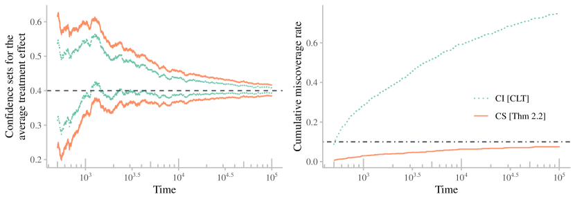
Figure 1: The left plot shows one run of a single experiment: a time-uniform CS alongside a fixed-time CI for a parameter of interest (in this case, the average treatment effect (ATE) of 0.4, an example we expand on in Section 3). The true value of the ATE is covered by the CS simultaneously from time 30 to 10000. On the other hand, the CI fails to cover the true ATE at several points in time. By repeating such experiments hundreds of times, one obtains the right plot which displays the cumulative probability of miscoverage — i.e. the probability of the CS or CI failing to capture the true ATE at any time up to $t$. Notice that the CI error rate begins at $\alpha=0.1$ and quickly grows, while the CS error rate never exceeds $\alpha=0.1$ (and never will, even asymptotically).

As mentioned before, while nonparametric CSs have been developed for several problems, they have thus far been nonasymptotic. Nonasymptotic inference for means of random variables requires strong assumptions on the distribution of the data [1]. These assumptions often take the form of a parametric likelihood [64, 17], known bounds on the random variables themselves [19, 65], on their moments [63], or on their moment generating functions [19].

These added distributional assumptions make existing CSs to be quite unlike CLT-based CIs which (a) are universal, meaning they take the same form — up to a change in influence functions — and are computed in the same way for most problems, and (b) are often applicable even when no nonasymptotic CI is known, such as in doubly robust inference of causal effects in observational studies. Our work bridges this gap, bringing properties (a) and (b) to the anytime-valid sequential regime by making one simple modification to the usual CIs. Just as CLT-based CIs yield approximate inference for a wide variety of problems in fixed-$n$ settings, our paper yields the same for sequential settings.

1.2 Contributions and outline

The primary contributions of this paper are in rigorously defining “asymptotic confidence sequences” (AsympCSs) in Definition 2.1 and deriving explicit constructions thereof which are as easy to implement and apply as the CLT. Additionally, we develop a Lindeberg-type asymptotic CS that is able to capture time-varying means under martingale dependence (Section 2.4). In Section 2.5, we give a definition of asymptotic time-uniform coverage (akin to coverage of asymptotic CIs) and show how sequences of our AsympCSs have this property. In Section 3 we illustrate how the asymptotic CSs of Section 2.1 enable anytime-valid doubly robust inference of causal effects in both randomized experiments and observational studies (Section 3). To be clear, we are not focused on deriving new semiparametric estimators; we simply demonstrate how doubly robust causal inference — a problem for which no known CSs exist — can now be tackled in fully sequential environments using the existing state-of-the-art estimators combined with our time-uniform bounds (Theorems 3.1 and 3.2). In Section 4, we provide a simulation study to assess empirical widths and type-I error rates of our asymptotic CSs and compare them to some existing (nonasymptotic) CSs in the literature. Finally, we apply the asymptotic CSs of Section 3 to a real observational data set by sequentially estimating the effects of fluid intake on 30-day mortality in sepsis patients. In sum, this work greatly expands the scope of anytime-valid inference, and does so via technically nontrivial derivations.

2 Time-uniform central limit theory

We first define what it means for a sequence of intervals to form an asymptotic confidence sequence (AsympCS). Then, we derive a “universal” AsympCS in the sense that the AsympCS does not depend on any features of the distribution beyond its mean and variance. This universal AsympCS is fundamentally related to Gaussians — much like classical asymptotic confidence intervals based on the CLT — since it stems from Brownian motion approximations and so-called strong invariance principles. Finally, similar to CIs based on martingale CLTs, we derive a Lindeberg-type martingale AsympCS that can track a moving average of conditional means.

2.1 Defining asymptotic confidence sequences

As mentioned in Section 1, the literature on CSs has focused on the nonasymptotic regime where strong assumptions must be placed on the observed random variables, such as boundedness, a parametric likelihood, or upper bounds on their MGFs. On the other hand, in batch — i.e. fixed-time — statistical analyses, the CLT is routinely applied to obtain approximately valid CIs in large samples, as it requires weak finite moment assumptions and has a simple, universal closed-form expression. Here, we define and present “asymptotic confidence sequences” as time-uniform analogues of asymptotic CIs, making similarly weak moment assumptions and providing a universal closed-form boundary.

The term “asymptotic confidence sequence” may at first seem paradoxical. Indeed, ever since their introduction by Robbins and collaborators [10, 42, 28, 29], CSs have been defined nonasymptotically, satisfying the time-uniform guarantee in equation (2). So how could a bound be both time-uniform and asymptotically valid? We clarify this critical point soon, with an analogy to classical asymptotic CIs. Similar to asymptotic CIs, AsympCSs trade nonasymptotic guarantees for (a) simplicity and universality, and (b) the ability to tackle a much wider variety of problems, especially those for which there is no known nonasymptotic CS. Said differently, AsympCSs trade finite sample validity for versatility (exemplified in Section 3 with a particular emphasis on modern causal inference).

Indeed, there is a clear desire for time-uniform methods with CLT-like simplicity and versatility, especially in the context of causal inference. For example, Johari et al. [21, Section 4.3] use a Gaussian mixture sequential probability ratio test (SPRT) to conduct A/B tests (i.e. randomized experiments) for data coming from (non-Gaussian) exponential families and mentions that CLT approximations hold at large sample sizes. Similarly, Yu et al. [66] develop a mixture SPRT for causal effects in generalized linear models, where they say that their likelihood ratio forms an “approximate martingale”, meaning its conditional expectation is constant up to a factor of $\exp\left\{o_{\mathbb{P}}(1)\right\}$. Moreover, Pace and Salvan [34] suggest using Robbins’ Gaussian mixture CS as a closed-form “approximate CS” and they demonstrate through simulations that the time-uniform coverage guarantee tends to hold in the asymptotic regime. However, all of these approaches justify time-uniform inference with $o_{\mathbb{P}}(\cdot)$ approximations that only hold at a fixed, pre-specified sample size, and yet inferences are being carried out at data-dependent sample sizes. This section remedies the tension between fixed-$n$ approximations and time-uniform inference by defining AsympCSs such that Gaussian approximations must hold almost surely for all sample sizes simultaneously. The AsympCSs we define will also be valid in a wide range of nonparametric scenarios (beyond exponential families, parametric models, and so on).

To motivate the definition of an AsympCS that follows, let us briefly review the CLT in the batch (non-sequential) setting. Suppose $Y_{1},\dots,Y_{n}\sim\mathbb{P}$ with mean $\mathbb{E}(Y_{1})=\mu$ and variance $\operatorname{\mathrm{var}}(Y_{1})=\sigma^{2}$. Then the standard CLT-based CI for $\mu$ takes the form

$$\dot{C}_{n}:=[\dot{L}_{n},\dot{U}_{n}]\equiv\left[\widehat{\mu}_{n}\pm\widehat{\sigma}_{n}\cdot\frac{\Phi^{-1}(1-\alpha/2)}{\sqrt{n}}\right],$$ (4)

where $\widehat{\mu}_{n}$ is the sample mean and $\Phi^{-1}(1-\alpha/2)$ is the $(1-\alpha/2)$-quantile of a standard Gaussian $N(0,1)$ (e.g. for $\alpha=0.05$, we have $\Phi^{-1}(0.975)\approx 1.96$). The classical notion of “asymptotic validity” is

$$\liminf_{n\to\infty}\mathbb{P}(\mu\in\dot{C}_{n})\geq 1-\alpha.$$ (5)

While the above is the standard definition of an asymptotic CI, we can arrive at a different definition by noting that a stronger statement can be made under the same conditions. Indeed, there exist iid standard Gaussians $Z_{1},\dots,Z_{n}\sim N(0,1)$ such that

$$\frac{1}{n}\sum_{i=1}^{n}(Y_{i}-\mu)/\sigma=\frac{1}{n}\sum_{i=1}^{n}Z_{i}+o_{\mathbb{P}}(1/\sqrt{n}).$$ (6)

Thus, one could define $[\dot{L}_{n},\dot{U}_{n}]$ to be an asymptotic $(1-\alpha)$-CI if there exists some (unknown) nonasymptotic $(1-\alpha)$-CI $[\dot{L}_{n}^{\star},\dot{U}_{n}^{\star}]$ such that

$$\dot{L}_{n}^{\star}/\dot{L}_{n}\xrightarrow{\mathbb{P}}1\quad\text{and}\quad\dot{U}_{n}^{\star}/\dot{U}_{n}\xrightarrow{\mathbb{P}}1$$ (7)

Statements of the form (6) are known as “couplings” and appear in the literature on strong approximations and invariance principles [14, 26, 27]. While justifications and derivations of CLT-based CIs like (4) are not typically presented using couplings, it is indeed the case that (6) implies the classical asymptotic validity guarantee (5). However, we deliberately highlight the alternative definition of asymptotic CIs because it ends up serving as a more natural starting point for defining asymptotic confidence sequences. In particular, we will define asymptotic CSs so that the approximation (7) holds uniformly over time, almost surely (though we do so using a slightly more general setup).

Definition 2.1 (Asymptotic confidence sequences).

Let $\mathcal{T}$ be a totally ordered infinite set including a minimum value $t_{0}\in\mathcal{T}$. We say that $[\widetilde{L}_{t},\widetilde{U}_{t}]_{t\in\mathcal{T}}$ is a $(1-\alpha)$-asymptotic confidence sequence (AsympCS) for a sequence of parameters $\widetilde{\theta}_{t}$ if there exists a (typically unknown) nonasymptotic $(1-\alpha)$-CS $[\widetilde{L}_{t}^{\star},\widetilde{U}_{t}^{\star}]_{t\in\mathcal{T}}$ for $\widetilde{\theta}_{t}$ — i.e. satisfying

$$\mathbb{P}\left(\forall t\in\mathcal{T},\ \widetilde{\theta}_{t}\in[\widetilde{L}_{t}^{\star},\widetilde{U}_{t}^{\star}]\right)\geq 1-\alpha,$$ (8)

and such that $[\widetilde{L}_{t},\widetilde{U}_{t}]$ becomes an arbitrarily precise almost-sure approximation to $[\widetilde{L}_{t}^{\star},\widetilde{U}_{t}^{\star}]$:

$$\widetilde{L}_{t}^{\star}/\widetilde{L}_{t}\xrightarrow{\mathrm{a.s.}}1\quad\text{and}\quad\widetilde{U}_{t}^{\star}/\widetilde{U}_{t}\xrightarrow{\mathrm{a.s.}}1.$$ (9)

In words, Definition 2.1 says that an AsympCS $[\widetilde{L}_{t},\widetilde{U}_{t}]_{t=1}^{\infty}$ is an arbitrarily precise approximation of some nonasymptotic CS $[\widetilde{L}_{t}^{\star},\widetilde{U}_{t}^{\star}]_{t=1}^{\infty}$ as $t\to\infty$ — capturing the intuition of having a time-uniform validity in large samples. Throughout the paper, we will mostly focus on the case where $\mathcal{T}=\{1,2,\dots\}$ and $t_{0}=1$.

It is important to note that alternate definitions to ours fail to be coherent in different ways. As one example, we could have hypothetically defined a sequence of intervals $C_{t}(\alpha)\equiv[L_{t},U_{t}]_{t=1}^{\infty}$ to be a $(1-\alpha)$-AsympCS if $\limsup_{m\to\infty}\mathbb{P}(\exists t\geq m:\mu\notin C_{t}(\alpha))\leq\alpha$, analogously to asymptotic CIs which satisfy $\limsup_{m\to\infty}\mathbb{P}(\mu\notin\dot{C}_{m}(\alpha))\leq\alpha$. In words, we could have posited that if we just start peeking late enough, then the probability of eventual miscoverage would indeed be below $\alpha$. Unfortunately, even for nonasymptotic CSs constructed at any level $\alpha^{\prime}\in(0,1)$, the former limit is zero, so this inequality would be vacuously true, regardless of $\alpha^{\prime}$, even if $\alpha^{\prime}\gg\alpha$. (Ideally, a nonasymptotic $(1-\alpha^{\prime})$ CS should also be an $(1-\alpha^{\prime})$-AsympCS for any $\alpha^{\prime}\leq\alpha$, but not an asymptotic $(1-\alpha)$-AsympCS for every $\alpha$.) However, we do show that sequences of our AsympCSs have a guarantee of this type if peeking starts late enough (see Section 2.5), but we delay these definitions until later as they are more involved.

Remark 1 (Why almost surely?).

One may wonder why it is necessary to define AsympCSs so that $\widetilde{L}_{t}^{\star}/\widetilde{L}_{t}\to 1$ almost surely (rather than in probability, for example). Since CSs are bounds that hold uniformly over time with high probability, convergence in probability $\widetilde{L}_{t}^{\star}/\widetilde{L}_{t}=1+o_{\mathbb{P}}(1)$ is not the right notion of convergence, as it only requires that the approximation term $o_{\mathbb{P}}(1)$ be small with high probability for sufficiently large fixed $t$, but not for all $t$ uniformly. It is natural to try to extend convergence in probability to time-uniform convergence with high probability — i.e. $\sup_{k\geq t}(\widetilde{L}_{k}^{\star}/\widetilde{L}_{k})=1+o_{\mathbb{P}}(1)$ — but it turns out (Section B.3) that this is equivalent to almost-sure convergence $\widetilde{L}_{t}^{\star}/\widetilde{L}_{t}=1+o_{\mathrm{a.s.}}(1)$.

Going forward, we may omit “a.s.” from ${o_{\mathrm{a.s.}}(\cdot)}$ and ${O_{\mathrm{a.s.}}(\cdot)}$ and instead simply write $o(\cdot)$ and $O(\cdot)$, respectively to simplify notation. Now that we have defined AsympCSs as time-uniform analogues of asymptotic CIs, we will explicitly derive AsympCSs for the mean of iid random variables with finite variances (i.e. under the same assumptions as the CLT).

2.2 Warmup: AsympCSs for the mean of iid random variables

We now construct an explicit AsympCS for the mean of iid random variables by combining a variant of Robbins’ (nonasymptotic) Gaussian mixture boundary [41] with Strassen’s strong approximation theorem [50]. Before presenting the main result, let us review both Robbins’ boundary and Strassen’s result, and discuss how they can be used in conjunction to arrive at the AsympCS in Theorem 2.2.

2.2.1 Robbins’ Gaussian mixture boundary

The study of CSs began with Herbert Robbins and colleagues [10, 41, 42, 28, 29], leading to several fundamental results and techniques including the famous Gaussian mixture boundary for partial sums of iid Gaussian random variables [41] (see also Howard et al. [19, §3.2]) which we recall here. Suppose $(Z_{t})_{t=1}^{\infty}$ are iid standard Gaussian random variables. Then for any $\rho>0$,

$$\mathbb{P}\left(\exists t\geq 1:\left\lvert\sum_{i=1}^{t}Z_{i}\right\rvert\geq\sqrt{\frac{2(t\rho^{2}+1)}{t^{2}\rho^{2}}\log\left(\frac{\sqrt{t\rho^{2}+1}}{\alpha}\right)}\right)\leq\alpha.$$ (10)

Notice that the above boundary scales as $O(\sqrt{t\log t})$ for any $\rho>0$. In fact, Robbins [41, Eq. 11] noted that (10) holds not only for Gaussian random variables, but for those that are $1$-sub-Gaussian, and hence pre-multiplying the boundary by $\sigma$ yields a $\sigma$-sub-Gaussian time-uniform concentration inequality, serving as a time-uniform analogue of Chernoff or Hoeffding inequalities. The connections between these fixed-time and time-uniform concentration inequalities are made explicit in Howard et al. [19]. Nevertheless, Eq. 10 requires a priori knowledge of $\sigma>0$ unlike CLT-based CIs which we aim to emulate in the time-uniform regime. The following strong Gaussian approximation due to Strassen [50] will serve as a technical tool allowing the nonasymptotic sub-Gaussian bound in (10) to be applied to partial sums of arbitrary random variables with finite variances.

2.2.2 Strassen’s strong approximation

Strassen [50] initiated the study of strong approximation (also called strong invariance principles or strong embeddings) which blossomed into an active and impactful corner of probability theory research over the subsequent years, culminating in now-classical results such as the Komlós-Major-Tusnády embeddings [26, 27, 31] and other related works [51, 13, 32, 7].

In his 1964 paper, Strassen [50, §2] used the Skorokhod embedding [49] (see also [4, p. 513]) to obtain the following strong invariance principle which connects asymptotic Gaussian behavior with the law of the iterated logarithm. Concretely, let $(Y_{t})_{t=1}^{\infty}$ be an infinite sequence of iid random variables from a distribution $\mathbb{P}$ with mean $\mu$ and variance $\sigma^{2}$. Then on a potentially richer probability space, there exist standard Gaussian random variables $(Z_{t})_{t=1}^{\infty}$ whose partial sums are almost-surely coupled with those of $(Y_{t})_{t=1}^{\infty}$ up to iterated logarithm rates, i.e.

$$\left\lvert\sum_{i=1}^{t}(Y_{i}-\mu)/\sigma-\sum_{i=1}^{t}Z_{i}\right\rvert=o\left(\sqrt{t\log\log t}\right)\quad\text{almost surely.}$$ (11)

Notice that the law of the iterated logarithm states that $|\sum_{i=1}^{t}(Y_{i}-\mu)/\sigma|=O(\sqrt{t\log\log t})$ while (11) states that the same partial sum is almost-surely coupled with an implicit Gaussian process — i.e. replacing $O(\cdot)$ with $o(\cdot)$. It may be convenient to divide by $t$ and interpret (11) on the level of sample averages rather than partial sums, in which case the right-hand side becomes $o(\sqrt{\log\log t/t})$. Let us now describe how Strassen’s strong approximation can be combined with Robbins’ Gaussian mixture boundary to derive an AsympCS under finite moment assumptions akin to the CLT.

2.2.3 The Gaussian mixture asymptotic confidence sequence

Given the juxtaposition of (10) and (11), the high-level approach to the derivation of AsympCSs becomes clearer. Indeed, the essential idea behind Theorem 2.2 is as follows. By Strassen’s strong approximation, we couple the partial sums $S_{t}:=\sum_{i=1}^{t}(Y_{i}-\mu)/\sigma$ with implicit partial sums $G_{t}:=\sum_{i=1}^{t}Z_{i}$ of Gaussians $(Z_{t})_{t=1}^{\infty}$, and then use Robbins’ mixture boundary to obtain a time-uniform high-probability bound on the deviations of $|G_{t}|$, noting that the coupling rate $o(\sqrt{t\log\log t})$ is asymptotically dominated by the concentration rate $O(\sqrt{t\log t})$, leading to asymptotic validity in the formal sense of Definition 2.1.

Theorem 2.2 (Gaussian mixture asymptotic confidence sequence).

Suppose $(Y_{t})_{t=1}^{\infty}\sim\mathbb{P}$ is an infinite sequence of iid observations from a distribution $\mathbb{P}$ with mean $\mu$ and finite variance. Let $\widehat{\mu}_{t}:=\frac{1}{t}\sum_{i=1}^{t}Y_{i}$ be the sample mean, and $\widehat{\sigma}_{t}^{2}:=\frac{1}{t}\sum_{i=1}^{t}Y_{i}^{2}-(\widehat{\mu}_{t})^{2}$ the sample variance based on the first $t$ observations. Then, for any prespecified constant $\rho>0$,

$$\widebar{C}_{t}^{\mathcal{G}}\equiv(\widehat{\mu}_{t}\pm\widebar{\mathfrak{B}}_{t}^{\mathcal{G}}):=\left(\widehat{\mu}_{t}\pm\widehat{\sigma}_{t}\sqrt{\frac{2(t\rho^{2}+1)}{t^{2}\rho^{2}}\log\left(\frac{\sqrt{t\rho^{2}+1}}{\alpha}\right)}\right)$$ (12)

forms a $(1-\alpha)$-AsympCS for $\mu$.

The full proof of Theorem 2.2 can be found in Appendix A.1. We can think of $\rho>0$ as a user-chosen tuning parameter which dictates the time at which (12) is tightest, and we discuss how to easily tune this value in Section B.2. A one-sided analogue of (12) can be found in Section B.1.

While (12) may look visually similar to Robbins’ (sub)-Gaussian mixture CS [41] — written explicitly in Howard et al. [19, Eq. (14)] — it is worth pausing to reflect on how they are markedly different. Firstly, Robbins’ CS is a nonasymptotic bound that is only valid for $\sigma$-sub-Gaussian random variables, meaning $\mathbb{E}\exp\{\lambda Y_{1}\}\leq\exp\{\sigma^{2}\lambda^{2}/2\}$ for some a priori known $\sigma>0$, while Theorem 2.2 does not require the existence of a finite MGF at all (much less a known upper bound on it). Secondly, Robbins’ CS uses this known (possibly conservative) $\sigma$ in place of $\widehat{\sigma}_{t}$ in (12), and thus it cannot adapt to an unknown variance, while (12) always scales with $\sqrt{\operatorname{\mathrm{var}}(Y_{1})}$. In simpler terms, Theorem 2.2 is a time-uniform analogue of the CLT in the same way that Robbins’ CS is a time-uniform analogue of a sub-Gaussian concentration inequality (e.g. Hoeffding’s or Chernoff’s inequality [16, 18]).

It is important not to confuse Theorem 2.2 with a martingale CLT as the latter still gives fixed-time CIs in the spirit of the usual CLT but under different assumptions on the martingale difference sequence (however, we do present an analogue of Theorem 2.2 under martingale dependence in Theorem 2.5).

2.2.4 An asymptotic confidence sequence with iterated logarithm rates

As a consequence of the law of the iterated logarithm, a confidence sequence for $\mu$ centered at $\widehat{\mu}_{t}$ cannot have an asymptotic width smaller than $O(\sqrt{\log\log t/t})$. This is easy to see since

$$\limsup_{t\to\infty}\frac{\sqrt{t}|\widehat{\mu}_{t}-\mu|}{\sigma\sqrt{2\log\log t}}=1.$$

This raises the question as to whether $\widebar{C}_{t}^{\mathcal{G}}$ can be improved so that the optimal asymptotic width of $O(\sqrt{\log\log t/t})$ is achieved. Indeed, we can replace Robbins’ Gaussian mixture boundary with Howard et al. [19, Eq. (2)] (or virtually any other Gaussian boundary for that matter) in the proof of Theorem 2.2 to derive such an AsympCS, but as the authors discuss, mixture boundaries such as the one in Theorem 2.2 may be preferable in practice, because any bound that is tighter “later on” (asymptotically) must be looser “early on” (at practical sample sizes) due to the fact that all such bounds have a cumulative miscoverage probability $\leq\alpha$. Nevertheless, we present an AsympCS with an iterated logarithm rate here for completeness.

Proposition 2.3 (Iterated logarithm asymptotic confidence sequences).

Under the same conditions as Theorem 2.2,

$$\widebar{C}_{t}^{\mathcal{L}}\equiv(\widehat{\mu}_{t}\pm\widebar{\mathfrak{B}}_{t}^{\mathcal{L}}):=\left(\widehat{\mu}_{t}\pm\widehat{\sigma}_{t}\cdot 1.7\sqrt{\frac{\log\log(2t)+0.72\log(10.4/\alpha)}{t}}\right)$$

forms a $(1-\alpha)$-AsympCS for $\mu$ with the same rate $r_{t}$ as in Theorem 2.2.

We omit the proof of Proposition 2.3 as it proceeds in a similar fashion to that of Theorem 2.2. In fact, both of these AsympCSs are simply instantiations of a more general principle for deriving AsympCSs by combining strong approximations with time-uniform boundaries for the approximating process, an approach that we discuss in the following section.

2.3 A general framework for deriving asymptotic confidence sequences

The proofs of both Theorem 2.2 and Proposition 2.3 follow the same general structure, combining strong approximations with time-uniform boundaries along with some other almost-sure asymptotic behavior. Abstracting away the details specific to these particular results, we provide the following four general conditions under which many AsympCSs can be derived, including those from the previous section but also Lyapunov- and Lindeberg-type AsympCS that we will derive in Section 2.4).

In what follows, let $\mathcal{T}$ be a totally ordered infinite set that includes a minimum value $t_{0}\in\mathcal{T}$ (for example, one may think about $\mathcal{T}$ as $\mathbb{R}^{\geq 0}$ or $\mathbb{N}$ with $t_{0}=0$). Then, consider the following four conditions where we use the “Condition G-X” enumeration as a mnemonic for the X${}^{\text{th}}$ condition in the section on General frameworks for AsympCSs).

Condition G-1 (Strong approximation).

On a potentially enriched probability space, there exists a process $(Z_{t})_{t\in\mathcal{T}}$ starting at $Z_{t_{0}}\equiv 0$ that strongly approximates $(\widehat{\theta}_{t}-\theta_{t})_{t\in\mathcal{T}}$ up to a rate of $(r_{t})_{t\in\mathcal{T}}$, i.e.

$$(\widehat{\theta}_{t}-\theta_{t})-Z_{t}=O\left(r_{t}\right)\quad\text{almost surely}.$$ (13)

Condition G-2 (Boundary for the approximating process).

The process $[L_{t}^{\star},U_{t}^{\star}]_{t\in\mathcal{T}}$ forms a $(1-\alpha)$-boundary for the process $(Z_{t})_{t\in\mathcal{T}}$ given in (13):

$$\mathbb{P}\left(\forall t\in\mathcal{T},\ Z_{t}\in[L_{t},U_{t}]\right)\geq 1-\alpha.$$ (14)

Condition G-3 (Strong approximation rate).

The approximation rate $(r_{t})_{t\in\mathcal{T}}$ in (13) is faster than both $(L_{t})_{t\in\mathcal{T}}$ and $(U_{t})_{t\in\mathcal{T}}$ in (14), i.e.

$$r_{t}=o\left(|L_{t}|\land|U_{t}|\right)\quad\text{almost surely.}$$ (15)

Condition G-4 (Almost-sure approximate boundary).

The $(1-\alpha)$-boundary $[L_{t},U_{t}]_{t\in\mathcal{T}}$ for $(Z_{t})_{t\in\mathcal{T}}$ is almost-surely approximated by the sequences $[\widehat{L}_{t},\widehat{U}_{t}]_{t\in\mathcal{T}}$, i.e.

$$\widehat{L}_{t}/L_{t}\xrightarrow{\mathrm{a.s.}}1\quad\text{and}\quad\widehat{U}_{t}/U_{t}\xrightarrow{\mathrm{a.s.}}1.$$ (16)

Deriving new AsympCSs then reduces to the conceptually simpler but nevertheless nontrivial task of satisfying the requisite conditions above. For example, in the previous section, we satisfied G-1 via Strassen [50], G-2 via Robbins [41], G-3 via the combination of Strassen [50] and Robbins [41], and G-4 via the strong law of large numbers (SLLN). The only difference between Theorem 2.2 and Proposition 2.3 was in what boundaries were being used for $[L_{t},U_{t}]_{t\in\mathcal{T}}$ and $[\widehat{L}_{t},\widehat{U}_{t}]_{t\in\mathcal{T}}$. More generally under Sections G-1–G-4, we have the following abstract Lemma for AsympCSs.

Lemma 2.4 (An abstract AsympCS for well-approximated processes).

Let $\mathcal{T}$ be a totally ordered infinite set including $0$ (e.g. $\mathbb{N}^{\geq 0}$ or $\mathbb{R}$) with $(\widehat{\theta}_{t})_{t\in\mathcal{T}}$ a real-valued integrable process adapted to the filtration $(\mathcal{F}_{t})_{t\in\mathcal{T}}$. Under Sections G-1–G-4,

$$\left[\widehat{\theta}_{t}+L_{t},\widehat{\theta}_{t}+U_{t}\right]$$ (17)

forms a $(1-\alpha)$-AsympCS for $\theta_{t}$ meaning there exists some nonasymptotic $(1-\alpha)$-CS $[\widehat{\theta}_{t}+L_{t}^{\star},\widehat{\theta}_{t}+U_{t}^{\star}]_{t\in\mathcal{T}}$ for $(\theta_{t})_{t\in\mathcal{T}}$, i.e.

$$\mathbb{P}\left(\forall t\in\mathcal{T},\ \theta_{t}\in\left[\widehat{\theta}_{t}+L_{t}^{\star},\widehat{\theta}_{t}+U_{t}^{\star}\right]\right)\geq 1-\alpha$$ (18)

such that $L_{t}^{\star}/\widehat{L}_{t}\xrightarrow{\mathrm{a.s.}}1$ and $U_{t}^{\star}/\widehat{U}_{t}\xrightarrow{\mathrm{a.s.}}1$.

We provide a short proof of Lemma 2.4 in Section A.2. In the following section, we will use the general recipe of Lemma 2.4 to obtain AsympCSs for time-varying means from non-iid random variables under martingale dependence as in the Lindeberg CLT [30, 4].

2.4 Lindeberg- and Lyapunov-type AsympCSs for time-varying means

The results in Theorem 2.2 and Proposition 2.3 focused on the situation where the observed random variables are independent and identically distributed, as this is one of the most commonly studied regimes in statistical inference. In practice, however, we may not wish to assume that means and variances remain constant over time, or that observations are independent of each other. Nevertheless, an analogue of Theorem 2.2 still holds for random variables with time-varying means and variances under martingale dependence. In this case, rather than the CS covering some fixed $\mu$, it covers the average conditional mean thus far: $\widetilde{\mu}_{t}:=\frac{1}{t}\sum_{i=1}^{t}\mu_{i}$ — to be made precise shortly.

Given the additional complexity introduced by considering time-varying conditional distributions, we will first explicitly spell out the conditions required to achieve a time-varying analogue of Theorem 2.2. Note however, that these conditions are no more restrictive, meaning that they reduce to the conditions of Theorem 2.2 in the iid regime. Suppose $(Y_{t})_{t=1}^{\infty}$ is a sequence of random variables with conditional means and variances given by $\mu_{t}:=\mathbb{E}(Y_{t}\mid Y_{1}^{t-1})$ and $\sigma_{t}^{2}:=\operatorname{\mathrm{var}}(Y_{t}\mid Y_{1}^{t-1})$, respectively. First, we require that the average conditional variance $\widetilde{\sigma}_{t}^{2}:=\frac{1}{t}\sum_{i=1}^{t}\sigma_{i}^{2}$ either does not vanish, or does so superlinearly; equivalently, we require that the cumulative conditional variance diverges.

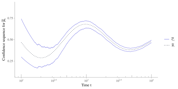
Figure 2: A $90\%$-AsympCS for the time-varying mean $\widetilde{\mu}_{t}$ using Theorem 2.5 with $\rho$ optimized for $t^{\star}=500$ based on the exact solution of Section B.2. Here, we have set $\mu_{t}:=\frac{1}{2}(1-\sin(2\log(e+10t))/\log(e+0.01t))$ to produce the sinusoidal behavior of $\widetilde{\mu}_{t}$. Notice that $\widetilde{C}_{t}$ uniformly captures $\widetilde{\mu}_{t}$, adapting to its non-stationarity.

Condition L-1 (Cumulative variance diverges almost surely).

For each $t\geq 1$, let $\sigma_{t}^{2}:=\operatorname{\mathrm{var}}(Y_{t}\mid Y_{1}^{t-1})$ be the conditional variance of $Y_{t}$. Then,

$$V_{t}:=\sum_{i=1}^{t}\sigma_{i}^{2}\to\infty~{}~{}\text{almost surely}.$$ (19)

Eq. 19 can also be interpreted as saying that the average conditional variance $\widetilde{\sigma}_{t}^{2}:=\frac{1}{t}\sum_{i=1}^{t}\sigma_{i}^{2}$ does not vanish faster than $1/t$ (if at all), meaning $\widetilde{\sigma}_{t}^{2}=\omega_{\mathrm{a.s.}}(1/t)$. For example, L-1 would hold if $\widetilde{\sigma}_{t}^{2}\xrightarrow{\mathrm{a.s.}}\sigma_{\star}^{2}$ for some $\sigma_{\star}^{2}>0$ or in the iid case where $\sigma^{2}_{1}=\sigma^{2}_{2}=\cdots=\sigma_{\star}^{2}$. Second, we require a Lindeberg-type uniform integrability condition on the tail behavior of $(Y_{t})_{t=1}^{\infty}$.

Condition L-2 (Lindeberg-type uniform integrability).

For each $t\geq 1$, let $\sigma_{t}^{2}:=\operatorname{\mathrm{var}}(Y_{t}\mid Y_{1}^{t-1})$ be the conditional variance of $Y_{t}$. Then there exists some $0<\kappa<1$ such that

$$\sum_{t=1}^{\infty}\frac{\mathbb{E}\left[(Y_{t}-\mu_{t})^{2}\mathds{1}\left((Y_{t}-\mu_{t})^{2}>V_{t}^{\kappa}\right)\mid Y_{1}^{t-1}\right]}{V_{t}^{\kappa}}<\infty~{}~{}\text{almost surely.}$$ (20)

Notice that Eq. 20 is satisfied if all conditional $q^{\mathrm{th}}$ moments are almost surely uniformly bounded for some $q>2$, meaning $1/K\leq\mathbb{E}(|Y_{t}-\mu_{t}|^{q}\mid Y_{1}^{t-1})<K$ a.s. for all $t\geq 1$ and for some constant $K>0$, or more generally under a Lyapunov-type condition that states $\sum_{t=1}^{\infty}\frac{\mathbb{E}(|Y_{t}-\mu_{t}|^{2+\delta}\mid Y_{1}^{t-1})}{\sqrt{V_{t}}^{2+\delta}}<\infty$ a.s. for some $\delta>0$. Third and finally, we require a consistent variance estimator.

Condition L-3 (Consistent variance estimation).

Let $\widehat{\sigma}_{t}^{2}$ be an estimator of $\widetilde{\sigma}_{t}^{2}$ constructed using $Y_{1},\dots,Y_{t}$ such that

$$\widehat{\sigma}_{t}^{2}/\widetilde{\sigma}_{t}^{2}\xrightarrow{\mathrm{a.s.}}1.$$ (21)

Note that in the iid case, (21) would hold using the sample variance by the SLLN. More generally for independent but non-identically distributed data, L-3 holds as long as the variation in means vanishes — i.e. $\frac{1}{t}\sum_{i=1}^{t}(\mu_{i}-\widetilde{\mu}_{t})^{2}=o(1)$ — but we will expand on this later in Corollary 2.6. Given Sections L-1, L-2, and L-3, we have the following AsympCS for the time-varying conditional mean $\widetilde{\mu}_{t}:=\frac{1}{t}\sum_{i=1}^{t}\mu_{i}$.

Theorem 2.5 (Lindeberg-type Gaussian mixture martingale AsympCS).

Let $(Y_{t})_{t=1}^{\infty}$ be a sequence of random variables with conditional mean $\mu_{t}:=\mathbb{E}(Y_{t}\mid Y_{1}^{t-1})$ and conditional variance $\sigma_{t}^{2}:=\operatorname{\mathrm{var}}(Y_{t}\mid Y_{1}^{t-1})$. Then under Assumptions L-1, L-2, and L-3, we have that

$$\widetilde{C}_{t}\equiv(\widehat{\mu}_{t}\pm\widetilde{\mathfrak{B}}_{t}):=\left(\widehat{\mu}_{t}\pm\sqrt{\frac{2(t\widehat{\sigma}_{t}^{2}\rho^{2}+1)}{t^{2}\rho^{2}}\log\left(\frac{\sqrt{t\widehat{\sigma}_{t}^{2}\rho^{2}+1}}{\alpha}\right)}\right)$$ (22)

forms a $(1-\alpha)$-AsympCS for the running average conditional mean $\widetilde{\mu}_{t}:=\frac{1}{t}\sum_{i=1}^{t}\mu_{i}$.

At a high level, the proof of Theorem 2.5 (found in Section A.3) follows from the general AsympCS procedure of Lemma 2.4 by using L-2 and Strassen’s 1967 strong approximation [51] (not to be confused with his 1964 result that we used in Theorem 2.2) to satisfy Conditions G-1 and G-3, and a variant of Robbins’ mixture martingale for non-iid random variables — that appears to be new in the literature — along with Conditions L-1 and L-3 to satisfy Conditions G-2 and G-4.

Notice that if the data happen to be iid, then $(\widetilde{C}_{t})_{t=1}^{\infty}$ is asymptotically equivalent to $(\widebar{C}_{t}^{\mathcal{G}})_{t=1}^{\infty}$ given in Theorem 2.2 (here, “asymptotic equivalence” simply means that the ratio of the two boundaries converges a.s. to 1). In other words, Theorem 2.5 is valid in a more general (non-iid) setting, but will essentially recover Theorem 2.2 in the iid case. Fig. 2 illustrates what $\widetilde{C}_{t}$ may look like in practice. Note that when $(Y_{t})_{t=1}^{\infty}$ are independent with $\mu_{1}=\mu_{2}=\cdots=\mu_{\star}$, and $\sigma_{1}^{2}=\sigma_{2}^{2}=\cdots=\sigma_{\star}^{2}$, it is nevertheless the case that $\widetilde{C}_{t}$ forms a $(1-\alpha)$-AsympCS for $\mu_{\star}$ under the same assumptions as Theorem 2.2. In this sense, we can view $(\widetilde{C}_{t})_{t=1}^{\infty}$ as “robust” to deviations from independence and stationarity. A one-sided analogue of Theorem 2.5 is presented in Proposition B.2 within Section B.1.

As a near-immediate corollary of Theorem 2.5, we have the following Lyapunov-type AsympCS under independent but non-identically distributed random variables.

Corollary 2.6 (Lyapunov-type AsympCS).

Suppose $(Y_{t})_{t=1}^{\infty}$ is a sequence of independent random variables with individual means and variances given by $\mu_{t}:=\mathbb{E}(Y_{t})$ and $\sigma_{t}^{2}:=\operatorname{\mathrm{var}}(Y_{t})$, respectively. Suppose that in addition to L-1 and the Lyapunov-type condition $\sum_{i=1}^{\infty}\frac{\mathbb{E}|Y_{i}-\mu_{i}|^{2+\delta}}{\sqrt{V_{i}}^{2+\delta}}<\infty$, we have the following regularity conditions:

$$\sum_{i=1}^{\infty}\frac{\mathbb{E}|Y_{i}^{2}-\mathbb{E}Y_{i}^{2}|^{1+\beta}}{V_{i}^{1+\beta}}<\infty,\quad\widetilde{\mu}_{t}^{2}=o(V_{t}),\quad\text{and}\quad\frac{1}{t}\sum_{i=1}^{t}(\mu_{i}-\widetilde{\mu}_{t})^{2}=o(\widetilde{\sigma}_{t}^{2})$$ (23)

for some $\beta\in(0,1)$. In other words, the higher moments of $(Y_{t})_{t=1}^{\infty}$, the running mean $\widetilde{\mu}_{t}$, and the “variation in means” $\frac{1}{t}\sum_{i=1}^{t}(\mu_{i}-\widetilde{\mu}_{t})^{2}$ all cannot diverge too quickly relative to $(V_{t})_{t=1}^{\infty}$. Then using the sample variance for $\widehat{\sigma}_{t}^{2}$, $\widetilde{C}_{t}$ forms a $(1-\alpha)$-AsympCS for the running average mean $\widetilde{\mu}_{t}:=\frac{1}{t}\sum_{i=1}^{t}\mu_{i}$.

Clearly, the conditions of (23) are trivially satisfied if means and variances are uniformly bounded over time. Since Sections L-1 and L-2 hold by the assumptions of Corollary 2.6, the proof in Section A.4 simply shows how the conditions in (23) imply L-3.

As suggested by Section 2.3, we can combine Lemma 2.4 with essentially any other Gaussian boundary, and indeed there are others that can yield Lindeberg- and Lyapunov-type AsympCSs but we do not enumerate any more here, though we do mention one inspired by Robbins [41, Eq. (20)] in passing in Section 2.6. The next section discusses how all of the aforementioned AsympCSs satisfy a certain formal asymptotic coverage guarantee.

2.5 Asymptotic coverage and type-I error control

While the AsympCSs derived thus far serve as sequential analogues of CLT-based CIs, it is not immediately obvious whether AsympCSs enjoy similar asymptotic coverage (equivalently, type-I error) guarantees. We will now give a positive answer to this question by showing that after appropriate tuning, our AsympCSs have asymptotic $(1-\alpha)$-coverage uniformly for all $t\geq m$ as $m\to\infty$ (to be formalized in Definition 2.7).

Recall that in the discussion preceding the definition of AsympCSs (Definition 2.1), we appealed to the rather strong fact that for an asymptotic confidence interval $\dot{C}_{n}:=(\widehat{\mu}_{n}\pm\dot{\mathfrak{B}}_{n})$, there exists a nonasymptotic CI $\dot{C}_{n}^{\star}:=(\widehat{\mu}_{n}\pm\dot{\mathfrak{B}}_{n}^{\star})$ such that $\dot{\mathfrak{B}}_{n}^{\star}/\dot{\mathfrak{B}}_{n}\xrightarrow{\mathbb{P}}1$. In particular we said that $\widebar{C}_{t}:=(\widehat{\mu}_{t}\pm\widebar{\mathfrak{B}}_{t})$ is an AsympCS if there exists a nonasymptotic CS $\widebar{C}_{t}^{\star}:=(\widehat{\mu}_{t}\pm\widebar{\mathfrak{B}}_{t}^{\star})$ such that $\widebar{\mathfrak{B}}_{t}^{\star}/\widebar{\mathfrak{B}}_{t}^{\star}\xrightarrow{\mathrm{a.s.}}1$. Placing these guarantees side-by-side, our definition of AsympCSs was motivated by the fact that

$$\underbrace{\widebar{\mathfrak{B}}_{t}^{\star}/\widebar{\mathfrak{B}}_{t}\xrightarrow{\mathrm{a.s.}}1}_{\text{Asymptotic CS{}}}\quad\text{is a time-uniform analogue of}\quad\underbrace{\dot{\mathfrak{B}}_{n}^{\star}/\dot{\mathfrak{B}}_{n}\xrightarrow{\mathbb{P}}1}_{\text{Asymptotic CI{}}}.$$ (24)

However, another property of asymptotic CIs is that their coverage is at least $(1-\alpha)$ in the limit:

$$\liminf_{n\to\infty}\mathbb{P}(\mu\in\dot{C}_{n})\geq 1-\alpha,$$ (25)

but what is the time-uniform analogue of (25)? Since any single AsympCS will simply have some coverage, we provide the following definition as a time-uniform analogue of (25) for sequences of AsympCSs that start later and later.

Definition 2.7 (Asymptotic time-uniform coverage).

Let $(\widebar{C}_{t}(m))_{t=1}^{\infty}$ be a sequence of AsympCSs for $m=1,2,3\dots$ and let $\alpha\in(0,1)$. We say that $(\widebar{C}_{t}(m))_{t=1}^{\infty}$ has asymptotic time-uniform $(1-\alpha)$-coverage for $\mu$ if

$$\lim_{m\to\infty}\mathbb{P}(\forall t\geq m,\ \mu\in\widebar{C}_{t}(m))\geq 1-\alpha,$$ (26)

and we say that this coverage is sharp if the above inequality $(\geq 1-\alpha)$ is an equality $(=1-\alpha)$.

To the best of our knowledge, the existing literature lacks a concrete definition of asymptotic time-uniform coverage (or type-I error control) like Definition 2.7, but sequences of AsympCSs satisfying (26) have been implicit in Robbins [41] and Robbins and Siegmund [42] as well as the recent preprint of Bibaut et al. [2]. However, these prior works use boundaries that do not resemble those in the present paper, and hence it is an open question as to whether our AsympCSs satisfy Definition 2.7 in some sense. In the remainder of this section, we give a positive answer to this open question by providing (sharp) coverage guarantees for our AsympCSs. Furthermore, in Section 2.6 we will strictly improve on aforementioned bounds by Robbins [41], Robbins and Siegmund [42], and Bibaut et al. [2] by uniformly tightening their AsympCSs and weakening their assumptions, obtaining those bounds as corollaries.

In order to obtain asymptotic time-uniform coverage, we will need a stronger variant of L-3 so that variances are estimated at polynomial rates (rather than at arbitrary rates).

Condition L-3-$\eta$ (Polynomial rate variance estimation).

There exists some $0<\eta<1$ such that

$$\widehat{\sigma}_{t}^{2}-\widetilde{\sigma}_{t}^{2}=o\left(\frac{(t\widetilde{\sigma}_{t}^{2})^{\eta}}{t}\right)\quad\text{almost surely}.$$ (27)

Note that while L-3-$\eta$ is stronger than L-3, it is still quite mild. For instance, if $\widetilde{\sigma}_{t}^{2}$ is uniformly bounded, then (27) simply requires that $\widehat{\sigma}_{t}^{2}-\widetilde{\sigma}_{t}^{2}=o(t^{\eta-1})$ (i.e. at any polynomial rate, potentially much slower than $t^{-1/2}$). Moreover, in the iid case with at least $(2+\delta)$ finite absolute moments, L-3-$\eta$ always holds by the non-iid Marcinkiewicz-Zygmund SLLN (see [35, p. 272]).

Our goal now is to show that sequences of AsympCSs given in Theorem 2.5 have asymptotic time-uniform coverage, and we will achieve this by effectively tuning them for later and later start times. Recall that Section B.2 allows us to choose the parameter $\rho>0$ so that the AsympCS is tightest at some particular time — we will now choose $\rho_{m}$ based on the first peeking time $m$ as

$$\rho_{m}:=\rho(\widehat{\sigma}_{m}^{2}m\log(m\lor e))\equiv\sqrt{\frac{-2\log\alpha+\log(-2\log\alpha)+1}{\widehat{\sigma}_{m}^{2}m\log(m\lor e)}}.$$ (28)

Then, let $(\widetilde{C}_{t}(m))_{t=m}^{\infty}$ be the Gaussian mixture AsympCS with $\rho_{m}$ plugged into the expression of the boundary for all $t\geq m$:

$$\widetilde{C}_{t}(m):=\left(\widehat{\mu}_{t}\pm\sqrt{\frac{2(t\widehat{\sigma}_{t}^{2}\rho_{m}^{2}+1)}{t^{2}\rho_{m}^{2}}\log\left(\frac{\sqrt{t\widehat{\sigma}_{t}^{2}\rho_{m}^{2}+1}}{\alpha}\right)}\right).$$ (29)

In other words, $(\widetilde{C}_{t}(m))_{t=m}^{\infty}$ should be thought of as an AsympCS that only starts after time $m$, and is vacuous beforehand. The following theorem formalizes the coverage guarantees satisfied by this sequence of AsympCSs as $m\to\infty$.

Theorem 2.8 (Asymptotic $(1-\alpha)$-coverage for Gaussian mixture AsympCSs).

Given the same setup as Theorem 2.5 and Sections L-1, L-2, and  L-3-$\eta$, the AsympCSs $(\widetilde{C}_{t}(m))_{t=m}^{\infty}$ given in (29) have sharp asymptotic $(1-\alpha)$-coverage for $\widetilde{\mu}_{t}:=\frac{1}{t}\sum_{i=1}^{t}\mu_{i}$ as $m\to\infty$, meaning

$$\lim_{m\to\infty}\mathbb{P}\left(\forall t\geq m,\ \widetilde{\mu}_{t}\in\widetilde{C}_{t}(m)\right)=1-\alpha.$$ (30)

The proof can be found in Section A.7. Notice that in the iid setting, as $m\to\infty$, $(\widetilde{C}_{t}(m))_{t=m}^{\infty}$ is asymptotically equivalent to $(\widebar{C}_{t}^{\mathcal{G}}(m))_{t=m}^{\infty}$ given by

$$\widebar{C}_{t}^{\mathcal{G}}(m):=\left(\widehat{\mu}_{t}\pm\widehat{\sigma}_{t}\sqrt{\frac{2(t\widebar{\rho}_{m}^{2}+1)}{t^{2}\widebar{\rho}_{m}^{2}}\log\left(\frac{\sqrt{t\widebar{\rho}_{m}^{2}+1}}{\alpha}\right)}\right)$$ (31)

where $\widebar{\rho}_{m}:=\rho(m\log(m\lor e))$. A quick inspection of the proof will reveal that (31) also satisfies the coverage guarantee provided in Theorem 2.8 under the condition that $\widetilde{\sigma}_{t}^{2}\to\sigma_{\star}^{2}>0$. In summary, (31) can be thought of as an analogue of (29) for the AsympCSs that were derived in Theorem 2.2.

2.6 Asymptotic confidence sequences using Robbins’ delayed start

As is clear from Lemma 2.4, virtually any boundary for Gaussian observations can be used to derive an AsympCS as long as an appropriate strong invariance principle can be applied under the given assumptions — indeed, Theorem 2.2, Proposition 2.3, Theorem 2.5, and Corollary 2.6 are all instantiations of the general phenomenon outlined in Lemma 2.4.

Another AsympCS that may be of interest to practitioners is one that leverages Robbins’ CS for means of Gaussian random variables with a delayed start time [41, Eq. (20)]. In a nutshell, Robbins calculated a lower bound on the probability that a centered Gaussian random walk would remain within a particular two-sided boundary for all times $t\geq m$ given some starting time $m\geq 1$. That is, he showed that for iid standard Gaussians $(Z_{t})_{t=1}^{\infty}$, letting $G_{t}:=\sum_{i=1}^{t}Z_{i}$, and for any $a>0$,

$$\mathbb{P}\left(\forall t\geq m:\left\lvert G_{t}\right\rvert<\sqrt{t(a^{2}+\log(t/m))}\right)\geq 1-\Psi_{\pm}(a),$$ (32)

where $\Psi_{\pm}(a):=2(1-\Phi(a)+a\phi(a))$ and $\Phi$ and $\phi$ are the CDF and PDF of a standard Gaussian, respectively. In particular, setting $a\in(0,\infty)$ so that $\Psi_{\pm}(a)=\alpha$ yields a two-sided $(1-\alpha)$-boundary for the Gaussian random walk $(G_{t})_{t=1}^{\infty}$, and indeed, a solution to $\Psi_{\pm}(a)=\alpha$ always exists and is trivial to compute due to the fact that $\Psi_{\pm}$ is monotonically decreasing, starting at $\Psi_{\pm}(0)=1$ and $\lim_{a\to\infty}\Psi_{\pm}(a)=0$. In a followup paper, Robbins and Siegmund [42] extended the ideas of Robbins [41] to a large class of boundaries for Wiener processes so that the probabilistic inequality in (32) can be shown to be an equality when $|G_{t}|$ is replaced by the absolute value of a Wiener process (which would imply the inequality in (32) for iid standard Gaussians as a corollary). Using this fact within the general framework of Lemma 2.4 combined with the strong invariance principle of Strassen [51] and the techniques found in the proof of Theorem 2.8 yields the following result.

Proposition 2.9 (Delayed-start AsympCS).

Consider the same setup as Theorem 2.8 so that $(Y_{t})_{t=1}^{\infty}$ have conditional means and variances given by $\mu_{t}:=\mathbb{E}(Y_{t}\mid Y_{1},\dots,Y_{t-1})$ and $\sigma_{t}^{2}:=\operatorname{\mathrm{var}}(Y_{t}\mid Y_{1},\dots,Y_{t-1})$. Then under Section L-1, L-2, and L-3, we have that for any $m\geq 1$,

$$\widetilde{C}_{t}^{\mathrm{DS}}(m):=\left(\widehat{\mu}_{t}\pm\widehat{\sigma}_{t}\sqrt{\frac{1}{t}\left[a^{2}+\log\left(\frac{t\widehat{\sigma}_{t}^{2}}{m\widehat{\sigma}_{m}^{2}}\right)\right]}\right)\quad\text{if}~{}t\geq m$$ (33)

(and all of $\mathbb{R}$ otherwise) forms a $(1-\alpha)$-AsympCS for $\widetilde{\mu}_{t}$, where $a$ is chosen so that $\Psi_{\pm}(a)=\alpha$. Furthermore, under L-3-$\eta$, $\widetilde{C}_{t}^{\mathrm{DS}}(m)$ has sharp asymptotic time-uniform $(1-\alpha)$-coverage in the sense of Definition 2.7.

The proof is provided in Section A.9. Similar to the relationship between Theorem 2.8 and (31), we have that if variances happen to converge $\widetilde{\sigma}_{t}^{2}\to\sigma_{\star}^{2}>0$ almost surely, then as a corollary of Proposition 2.9, the sequence $(\widetilde{C}_{t}^{\mathrm{DS}\star}(m))_{t=1}^{\infty}$ given by

$$\widetilde{C}_{t}^{\mathrm{DS}\star}(m):=\left(\widehat{\mu}_{t}\pm\widehat{\sigma}_{t}\sqrt{\frac{1}{t}\left(a^{2}+\log\left(\frac{t}{m}\right)\right)}\right)\quad\text{for $t\geq m$}$$ (34)

has asymptotic time-uniform coverage as in Definition 2.7. This can be seen as a generalization and improvement of results implied by Robbins [41] and Robbins and Siegmund [42]. In followup work to ours by Bibaut et al. [2], the authors derive similar results to Robbins [41] and Robbins and Siegmund [42] yielding an AsympCS that can be written as a looser version of (34) (in fact, it was their paper that inspired us explicitly write down Definition 2.7 and to show that it holds more generally). We elaborate on the details of these connections in Section B.6.

3 Illustration: Causal effects and semiparametric estimation

Given the groundwork laid in Section 2, we now demonstrate the use of AsympCSs for conducting anytime-valid causal inference. Since it is an important and thoroughly studied functional, we place a particular emphasis on the average treatment effect (ATE) for illustrative purposes but we discuss how these techniques apply to semiparametric functional estimation more generally in Section 3.5. The literature on uncertainty quantification for semiparametric functional estimation often falls within the asymptotic regime and hence AsympCSs form a natural time-uniform extension thereof.

It is important to note that obtaining AsympCSs for the ATE is not as simple as directly applying the theorems of Section 2.1 to some appropriately chosen augmented inverse-probability-weighted (AIPW) influence functions (otherwise the illustration of this section would have been trivial). Indeed, satisfying the conditions of the aforementioned theorems — and Lemma 2.4 in particular — in the presence of potentially infinite-dimensional nuisance parameters is nontrivial and the analysis proceeds rather differently from the fixed-$n$ setting. Nevertheless, after introducing and carefully analyzing sequential sample-splitting and cross-fitting (Section 3.1), we will see that efficient time-uniform inference for the ATE is still possible.

To solidify the notation and problem setup, suppose that we observe a (potentially infinite) sequence of iid variables $Z_{1},Z_{2},\dots$ from a distribution $\mathbb{P}$ where $Z_{t}:=(X_{t},A_{t},Y_{t})$ denotes the $t^{\text{th}}$ subject’s triplet and $X_{t}\in\mathbb{R}^{d}$ are their measured baseline covariates, $A_{t}\in\{0,1\}$ is the treatment that they receive, and $Y_{t}\in\mathbb{R}$ is their measured outcome after treatment. Our target estimand is the average treatment effect (ATE) $\psi$ defined as

$$\psi:=\mathbb{E}(Y^{1}-Y^{0}).$$ (35)

where $Y^{a}$ is the counterfactual outcome for a randomly selected subject had they received treatment $a\in\{0,1\}$. The ATE $\psi$ can be interpreted as the average population outcome if everyone were treated $\mathbb{E}(Y^{1})$ versus if no one were treated $\mathbb{E}(Y^{0})$. Under standard causal identification assumptions — typically referred to as consistency, positivity, and exchangeability (see e.g. Kennedy [24, §2.2]) — we have that $\psi$ can be written as a (non-counterfactual) functional of the distribution $\mathbb{P}$:

$$\psi\equiv\psi(\mathbb{P})=\mathbb{E}\{\mathbb{E}(Y\mid X,A=1)-\mathbb{E}(Y\mid X,A=0)\}.$$ (36)

Throughout the remainder of this section, we will operate under these identification assumptions and aim to derive efficient AsympCSs for $\psi$ using tools from semiparametric theory. At a high level, we will construct AsympCSs for $\psi$ by combining the results of Section 2 with sample averages of influence functions for $\psi$ and in the ideal case, these influence functions will be efficient (in the semiparametric sense).

3.1 Sequential sample-splitting and cross-fitting

Following Robins et al. [43], Zheng and van der Laan [67], and Chernozhukov et al. [8], we employ sample-splitting to derive an estimate $\widehat{f}$ of the influence function $f$ on a “training” sample, and evaluate $\widehat{f}$ on values of $Z_{i}$ in an independent “evaluation” sample. Sample-splitting sidesteps complications introduced from “double-dipping” (i.e. using $Z_{i}$ to both construct $\widehat{f}$ and evaluate $\widehat{f}(Z_{i})$) and greatly simplifies the analysis of the downstream estimator. Since the aforementioned authors employed sample splitting in the batch (non-sequential) regime while we are concerned with settings where data are continually observed in an online stream over time, we modify the sample-splitting procedure as follows. We will denote ${\mathcal{D}}_{\infty}^{\mathrm{trn}}$ and ${\mathcal{D}}_{\infty}^{\mathrm{eval}}$ as the “training” and “evaluation” sets, respectively. At time $t$, we assign $Z_{t}$ to either group with equal probability:

$$Z_{t}\in\begin{cases}{\mathcal{D}}_{\infty}^{\mathrm{trn}}&\text{with probability }1/2,\\ {\mathcal{D}}_{\infty}^{\mathrm{eval}}&\text{otherwise.}\end{cases}$$

Note that at time $t+1$, $Z_{t}$ is not re-randomized into either split — once $Z_{t}$ is randomly assigned to one of ${\mathcal{D}}_{\infty}^{\mathrm{trn}}$ or ${\mathcal{D}}_{\infty}^{\mathrm{eval}}$, they remain in that split for the remainder of the study. In this way, we can write ${\mathcal{D}}_{\infty}^{\mathrm{trn}}=(Z_{1}^{\mathrm{trn}},Z_{2}^{\mathrm{trn}},\dots)$ and ${\mathcal{D}}_{\infty}^{\mathrm{eval}}=(Z_{1}^{\mathrm{eval}},Z_{2}^{\mathrm{eval}},\dots)$ and think of these as independent, sequential observations from a common distribution $\mathbb{P}$. To keep track of how many subjects have been randomized to ${\mathcal{D}}_{\infty}^{\mathrm{trn}}$ and ${\mathcal{D}}_{\infty}^{\mathrm{eval}}$ at time $t$, define

$${T}:=|{\mathcal{D}}_{\infty}^{\mathrm{eval}}|~{}~{}~{}\text{and}~{}~{}~{}{T^{\prime}}:=|{\mathcal{D}}_{\infty}^{\mathrm{trn}}|\equiv t-{T},$$ (37)

where we have left the dependence on $t$ implicit.

Figure 3: A schematic illustrating sequential sample splitting. At each time step $t$, the new observation $Z_{t}$ is randomly assigned to ${\mathcal{D}}_{\infty}^{\mathrm{trn}}$ or ${\mathcal{D}}_{\infty}^{\mathrm{eval}}$ with equal probability (1/2). Nuisance function estimators $(\widehat{\mu}_{{T^{\prime}}}^{1},\widehat{\mu}_{{T^{\prime}}}^{0},\widehat{\pi}_{{T^{\prime}}})$ are constructed using ${\mathcal{D}}_{\infty}^{\mathrm{trn}}$ which then yield $\widehat{f}_{{T^{\prime}}}$. The sample-split estimator $\widehat{\psi}_{t}^{\mathrm{split}}$ is defined as the sample average $\frac{1}{{T}}\sum_{i=1}^{T}\widehat{f}_{{T^{\prime}}}(Z_{i}^{\mathrm{eval}})$ where each $Z_{i}^{\mathrm{eval}}\in{\mathcal{D}}_{\infty}^{\mathrm{eval}}$.

Remark 2.

Strictly speaking, under the iid assumption, we do not need to randomly assign subjects to training and evaluation groups for the forthcoming results to hold (e.g. we could simply assign even-numbered subjects to ${\mathcal{D}}_{\infty}^{\mathrm{trn}}$ and odd-numbered subjects to ${\mathcal{D}}_{\infty}^{\mathrm{eval}}$). However, the analysis is not further complicated by this randomization, and it can be used to combat bias in treatment assignments when the iid assumption is violated [12].

3.1.1 The sequential sample-split estimators $(\widehat{\psi}_{t}^{\mathrm{split}})_{t=1}^{\infty}$

After employing sequential sample-splitting, the sequence of sample-split estimators $(\widehat{\psi}_{t}^{\mathrm{split}})_{t=1}^{\infty}$ for $\psi$ are given by

$$\widehat{\psi}_{t}^{\mathrm{split}}:=\frac{1}{{T}}\sum_{i=1}^{T}\widehat{f}_{{T^{\prime}}}(Z_{i}^{\mathrm{eval}}),$$ (38)

where $\widehat{f}_{{T^{\prime}}}$ is given by (188) with $\eta\equiv(\mu^{1},\mu^{0},\pi)$ replaced by $\widehat{\eta}_{{T^{\prime}}}\equiv(\widehat{\mu}^{1}_{{T^{\prime}}},\widehat{\mu}^{0}_{{T^{\prime}}},\widehat{\pi}_{{T^{\prime}}})$ which is built solely from ${\mathcal{D}}_{\infty}^{\mathrm{trn}}$. The sample-splitting procedure for constructing $\widehat{\psi}_{t}^{\mathrm{split}}$ is summarized pictorially in Fig. 3. In the batch setting for a fixed sample size, (38) is often referred to as the augmented inverse probability weighted (AIPW) estimator [45, 46] (an instantiation of so-called “one-step correction” in the semiparametrics literature) and we adopt similar nomenclature here.

3.1.2 The sequential cross-fit estimators $(\widehat{\psi}_{t}^{\times})_{t=1}^{\infty}$

A commonly cited downside of sample-splitting is the loss in efficiency by using ${T}\approx t/2$ subjects instead of $t$ when evaluating the sample mean $\frac{1}{{T}}\sum_{i=1}^{T}\widehat{f}_{{T^{\prime}}}(Z_{i}^{\mathrm{eval}})$. An easy fix is to cross-fit: swap the two samples, using the evaluation set ${\mathcal{D}}_{\infty}^{\mathrm{eval}}$ for training and the training set ${\mathcal{D}}_{\infty}^{\mathrm{trn}}$ for evaluation to recover the full sample size of $t\equiv{T}+{T^{\prime}}$ [43, 67, 8]. That is, construct $\widehat{f}_{T}$ solely from ${\mathcal{D}}_{\infty}^{\mathrm{eval}}$ and define the cross-fit estimator $\widehat{\psi}_{t}^{\times}$ as

$$\widehat{\psi}_{t}^{\times}:=\frac{\sum_{i=1}^{T}\widehat{f}_{{T^{\prime}}}(Z_{i}^{\mathrm{eval}})+\sum_{i=1}^{{T^{\prime}}}\widehat{f}_{{T}}(Z_{i}^{\mathrm{trn}})}{t},$$ (39)

and the associated cross-fit variance estimate

$$\widehat{\operatorname{\mathrm{var}}}_{t}(\widehat{f}):=\frac{\widehat{\operatorname{\mathrm{var}}}_{T}(\widehat{f}_{{T^{\prime}}})+\widehat{\operatorname{\mathrm{var}}}_{{T^{\prime}}}(\widehat{f}_{{T}})}{2},$$ (40)

where $\widehat{\operatorname{\mathrm{var}}}_{T}(\widehat{f}_{T^{\prime}})$ is the ${\mathcal{D}}_{\infty}^{\mathrm{eval}}$-sample variance of the pseudo-outcomes $(\widehat{f}_{{T^{\prime}}}(Z_{i}^{\mathrm{eval}}))_{t=1}^{{T}}$ at time $t$ and similarly for $\widehat{\operatorname{\mathrm{var}}}_{T^{\prime}}$ (we deliberately omit the subscript on $\widehat{f}$ in Eq. 40). All of the results that follow are stated in terms of the cross fit estimators $(\widehat{\psi}_{t}^{\times})_{t=1}^{\infty}$ but they also hold using $(\widehat{\psi}_{t}^{\mathrm{split}})_{t=1}^{\infty}$ instead. With the setup of Section B.7 and Section 3.1 in mind, we are ready to derive AsympCSs for $\psi$, first in randomized experiments.

3.2 Asymptotic confidence sequences in randomized experiments

Consider a sequential randomized experiment so that a subject with covariates $x$ has a known propensity score given by

$$\pi(x):=\mathbb{P}(A=1\mid X=x).$$

Consider the cross-fit AIPW estimator $\widehat{\psi}_{t}^{\times}$ as given in (39) but with estimated propensity scores — $\widehat{\pi}_{{T^{\prime}}}(x)$ and $\widehat{\pi}_{{T}}(x)$ — replaced by their true values $\pi(x)$, and with $\widehat{\mu}^{a}_{{T^{\prime}}}(x)$ and $\widehat{\mu}^{a}_{T}$ being possibly misspecified estimators for $\mu^{a}$. That is, we will assume that $\widehat{\mu}^{a}_{t}$ converges to some function $\widebar{\mu}^{a}$, which need not coincide with $\mu^{a}$. In what follows, when we use $\widehat{\mu}_{t}^{a}$ or $\widehat{f}_{t}$ in writing $\|\widehat{\mu}_{t}^{a}-\widebar{\mu}^{a}\|_{L_{2}(\mathbb{P})}$ or $\|\widehat{f}_{t}-\widebar{f}\|_{L_{2}(\mathbb{P})}$, we are referring to large-sample properties of the estimator (and hence $\widehat{f}_{t}$ could be replaced by $\widehat{f}_{T^{\prime}}$ or $\widehat{f}_{T}$ without loss of generality).

Theorem 3.1 (Confidence sequences for the ATE in randomized experiments).

Let $\widehat{\psi}_{t}^{\times}$ be the cross-fit AIPW estimator as in (39). Suppose $\|\widehat{\mu}^{a}_{t}(X)-\widebar{\mu}^{a}(X)\|_{L_{2}(\mathbb{P})}=o(1)$ for each $a\in\{0,1\}$ where $\widebar{\mu}^{a}$ is some function (but need not be $\mu^{a}$), and hence $\|\widehat{f}_{t}-\widebar{f}\|_{L_{2}(\mathbb{P})}=o(1)$ for some influence function $\widebar{f}$. Suppose that propensity scores are bounded away from 0 and 1, i.e. $\pi(X)\in[\delta,1-\delta]$ for some $\delta>0$, and suppose that $\mathbb{E}|\widebar{f}(Z)|^{4}<\infty$. Then for any constant $\rho>0$,

$$\widehat{\psi}_{t}^{\times}\pm\sqrt{\widehat{\operatorname{\mathrm{var}}}_{t}(\widehat{f})}\cdot\sqrt{\frac{2(t\rho^{2}+1)}{t^{2}\rho^{2}}\log\left(\frac{\sqrt{t\rho^{2}+1}}{\alpha}\right)}$$ (41)

forms a $(1-\alpha)$-AsympCS for $\psi$.

The proof in Appendix A.5 combines an analysis of the almost-sure convergence of $(\widehat{\psi}_{t}^{\times}-\psi)$ with the AsympCS of Theorem 2.2. Notice that since $\widehat{\mu}_{t}^{a}$ is consistent for a function $\widebar{\mu}^{a}$, we have that $\widehat{f}_{t}$ is converging to some influence function $\widebar{f}$ of the form

$$\widebar{f}(z)\equiv\widebar{f}(x,a,y):=\left\{\widebar{\mu}^{1}(x)-\widebar{\mu}^{0}(x)\right\}+\left(\frac{a}{\pi(x)}-\frac{1-a}{1-\pi(x)}\right)\left\{y-\widebar{\mu}^{a}(x)\right\}.$$ (42)

In practice, however, one must choose $\widehat{\mu}_{t}^{a}$. As alluded to at the beginning of Section 3, the best possible influence function is the EIF $f(z)$ defined in (188), and thus it is natural to attempt to construct $\widehat{\mu}_{t}^{a}$ so that $\|\widehat{f}_{t}-f\|_{L_{2}(\mathbb{P})}=o(1)$. The resulting confidence sequences would inherit such optimality properties, a point which we discuss further in Section B.8.

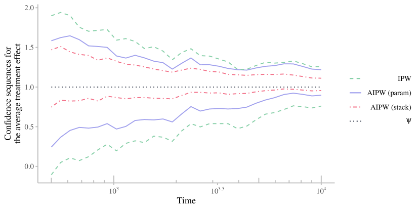
Figure 4: Three 90%-AsympCSs for the average treatment effect in a simulated randomized experiment using different regression estimators. Notice that all three confidence sequences uniformly capture the average treatment effect $\psi$, but increasingly sophisticated models do so more efficiently, with AIPW+stacking greatly outperforming IPW.

Since $\mu^{a}$ is simply a conditional mean function, we can use virtually any regression techniques to estimate it. Here we will consider the general approach of stacking introduced by Breiman [5] and further studied by Tsybakov [54] and van der Laan et al. [57] (see also [38, 39]) under the names of “aggregation” and “Super Learning” respectively. In short, stacking uses cross-validation to choose a weighted combination of $K$ candidate predictors where the weights are chosen based on data in held-out samples. Importantly, the candidate predictors can simultaneously include both flexible machine learning methods (e.g. random forests [6], generalized additive models [15], etc.) as well as simpler parametric ones and yet for large samples (and under certain conditions), the stacked predictor will have a mean squared error that scales with that of the best of the $K$ predictors up to an additive $\log K$ term [54, 60]. This advantage can be seen empirically in Fig. 4 where the true regression functions $\mu^{0}$ and $\mu^{1}$ are non-smooth and nonlinear in $x$. We wish to emphasize that such advantages via stacking are not new — we are only highlighting the observation that similar phenomena carry over to AsympCSs.

So far, the use of flexible regression techniques including the ensemble method of stacking were used only for the purposes of deriving sharper AsympCSs in sequential randomized experiments. In observational studies, however, consistent estimation of nuisance functions at fast rates is essential to the construction of valid fixed-$n$ CIs, and indeed the same is true for AsympCSs.

3.3 Asymptotic confidence sequences in observational studies

Consider now a sequential observational study (e.g. we are able to continuously monitor $(X_{t},A_{t},Y_{t})_{t=1}^{\infty}$ but do not know $\pi(x)$ exactly, or we are in a sequentially randomized experiment with noncompliance, etc.). The only difference in this setting with respect to setup is the fact that $\pi(x)$ is no longer known and must be estimated. As in the fixed-$n$ setting, however, this complicates estimation and inference. The following theorem provides the conditions under which we can construct AsympCSs for $\psi$ using the cross-fit AIPW estimator in observational studies.

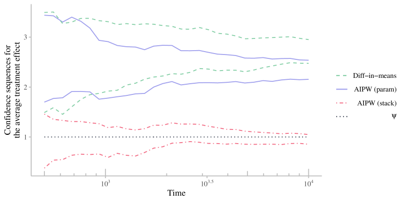
Figure 5: Three 90%-AsympCSs for the ATE in an observational study using three different estimators — a difference-in-means estimator, AIPW with parametric models, and AIPW with an ensemble of predictors combined via stacking. Unlike the randomized setup, only the stacking ensemble is consistent, since the other two are misspecified. Not only is the stacking-based AsympCS converging to $\psi$, but it is also the tightest of the three models at each time step.

Theorem 3.2 (Confidence sequence for the ATE in observational studies).

Consider the same setup as Theorem 3.1 but with $\pi(x)$ no longer known. Suppose that regression functions and propensity scores are consistently estimated in $L_{2}(\mathbb{P})$ at a product rate of $o(\sqrt{\log/t})$, meaning that

$$\|\widehat{\pi}_{t}-\pi\|_{L_{2}(\mathbb{P})}\sum_{a=0}^{1}\|\widehat{\mu}_{t}^{a}-\mu^{a}\|_{L_{2}(\mathbb{P})}=o\left(\sqrt{\log t/t}\right).$$

Moreover, suppose that $\|\widehat{f}_{t}-f\|_{L_{2}(\mathbb{P})}=o(1)$ where $f$ is the efficient influence function (188) and that $\mathbb{E}|f(Z)|^{4}<\infty$. Then for any constant $\rho>0$,

$$\widehat{\psi}_{t}^{\times}\pm\sqrt{\widehat{\operatorname{\mathrm{var}}}_{t}(\widehat{f})}\cdot\sqrt{\frac{2(t\rho^{2}+1)}{t^{2}\rho^{2}}\log\left(\frac{\sqrt{t\rho^{2}+1}}{\alpha}\right)}$$

forms a $(1-\alpha)$-AsympCS for $\psi$.

The proof in Appendix A.5.2 proceeds similarly to the proof of Theorem 3.1 by combining Theorem 2.2 with an analysis of the almost-sure behavior of $(\widehat{\psi}_{t}^{\times}-\psi)$. Notice that the nuisance estimation rate of $\sqrt{\log t/t}$ is slower than $1/\sqrt{t}$ which is usually required in the fixed-$n$ regime, but we do require almost-sure convergence rather than convergence in probability.

Unlike the experimental setting of Section 3.2, Theorem 3.2 requires that $\widehat{\mu}_{t}^{a}$ and $\widehat{\pi}_{t}$ consistently estimate $\mu^{a}$ and $\pi$, respectively. As a consequence, the stacking-based AIPW AsympCS is both the tightest of the three and is uniquely consistent for $\psi$ (see Fig. 5).

3.4 The running average of individual treatment effects

The results in Sections 3.2 and 3.3 considered the classical regime where the ATE $\psi$ is a fixed functional that does not change over time. Consider a strict generalization where distributions — and hence individual treatment effects in particular — may change over time. In other words,

$$\psi_{t}:=\mathbb{E}\left\{Y^{1}_{t}-Y^{0}_{t}\right\}\overset{(\star)}{=}\mathbb{E}\left\{\mathbb{E}(Y_{t}\mid X_{t},A_{t}=1)-\mathbb{E}(Y_{t}\mid X_{t},A_{t}=0)\right\},$$ (43)

where the equality $(\star)$ holds under the familiar causal identification assumptions discussed earlier. Despite the non-stationary and non-iid structure, it is nevertheless possible to derive AsympCSs for the running average of individual treatment effects $\widetilde{\psi}_{t}:=\frac{1}{t}\sum_{i=1}^{t}\psi_{i}$ — or simply, the running average treatment effect — using the Lyapunov-type bounds of Corollary 2.6. However, given this more general and complex setup, the assumptions required are more subtle (but no more restrictive) than those for Theorems 3.1 and 3.2; as such, we explicitly describe their details here but handle the randomized and observational settings simultaneously for brevity.

Condition $\widetilde{\text{ATE}}$-1 (Regression estimator is uniformly well-behaved in ${L_{2}(\mathbb{P})}$).

We assume that regression estimators $\mu_{t}^{a}(X_{i})$ converge in ${L_{2}(\mathbb{P})}$ to any function $\widebar{\mu}^{a}(X_{i})$ uniformly for $i\in\{1,2,\dots\}$ i.e.

$$\sup_{1\leq i<\infty}\|\widehat{\mu}_{t}^{a}(X_{i})-\widebar{\mu}^{a}(X_{i})\|_{L_{2}(\mathbb{P})}=o(1)$$ (44)

for each $a\in\{0,1\}$.

$\widetilde{\text{ATE}}$-1 simply requires that the regression estimator $\widehat{\mu}_{t}^{a}$ must converge to some function $\widebar{\mu}^{a}$, which need not coincide with true regression function $\mu^{a}$. In the iid setting where $X_{1},X_{2},\dots$ all have the same distribution, we would simply drop the $\sup_{1\leq i\leq\infty}$, recovering the conditions for Theorems 3.1 and 3.2.

Condition $\widetilde{\text{ATE}}$-2 (Convergence of average nuisance errors).

Let $\widehat{\mu}_{t}^{a}$ be an estimator of the regression function $\mu^{a}$, $a\in\{0,1\}$ and $\widehat{\pi}_{t}$ an estimator of the propensity score $\pi$. We assume that the average bias shrinks at a $\sqrt{\log t/t}$ rate, i.e.

$$\frac{1}{t}\sum_{i=1}^{t}\left\{\|\widehat{\pi}_{t}(X_{i})-\pi(X_{i})\|_{L_{2}(\mathbb{P})}\sum_{a=0}^{1}\|\widehat{\mu}_{t}^{a}(X_{i})-\mu^{a}(X_{i})\|_{L_{2}(\mathbb{P})}\right\}=o\left(\sqrt{\frac{\log t}{t}}\right).$$ (45)

Note that $\widetilde{\text{ATE}}$-2 would hold in two familiar scenarios. Firstly, in a randomized experiment (Theorem 3.3) where $\widehat{\pi}_{t}=\pi$ is known by design, we have that $\eqref{eq:doubly-robust-average-bias-convergence}$ is always zero, satisfying $\widetilde{\text{ATE}}$-2 trivially. Second, in an observational study where the product of errors $\|\widehat{\pi}_{t}(X_{i})-\pi(X_{i})\|_{L_{2}(\mathbb{P})}\|\widehat{\mu}_{t}^{a}(X_{i})-\mu^{a}(X_{i})\|_{L_{2}(\mathbb{P})}$ vanishes at a rate faster than $\sqrt{\log t/t}$, for each $i$ and for both $a\in\{0,1\}$, we also have that their average product errors vanish at the same rate (45). With these assumptions in mind, let us summarize how running average treatment effects can be captured in randomized experiments.

Theorem 3.3 (AsympCSs for the running average treatment effect).

Suppose $Z_{1},Z_{2},\dots$ are independent triples $Z_{t}:=(X_{t},A_{t},Y_{t})$ and that Sections $\widetilde{\text{ATE}}$-1 and $\widetilde{\text{ATE}}$-2 hold. Finally, suppose that the conditions of Corollary 2.6 hold, but with $(Y_{t})_{t=1}^{\infty}$ replaced by the influence functions $(\widebar{f}(Z_{t}))_{t=1}^{\infty}$. Then,

$$\widehat{\psi}_{t}^{\times}\pm\sqrt{\frac{2(t\rho^{2}\widehat{\operatorname{\mathrm{var}}}_{t}(\widebar{f})+1)}{t^{2}\rho^{2}}\log\left(\frac{\sqrt{t\rho^{2}\widehat{\operatorname{\mathrm{var}}}_{t}(\widebar{f})+1}}{\alpha}\right)}$$ (46)

forms a $(1-\alpha)$-AsympCS for the running average treatment effect $\widetilde{\psi}_{t}:=\frac{1}{t}\sum_{i=1}^{t}\psi_{i}$.

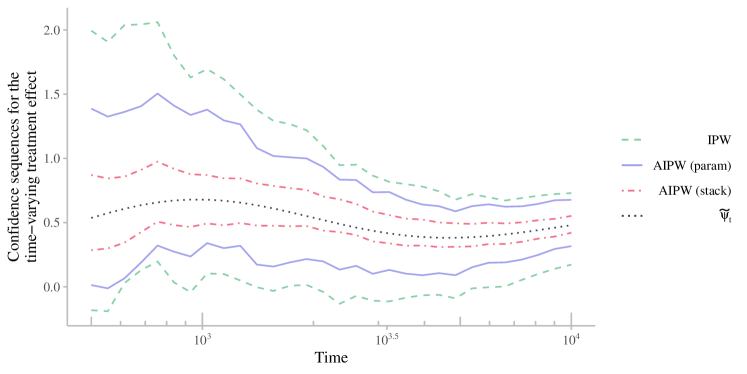
Figure 6: Three 90% AsympCSs for $\widetilde{\psi}_{t}$ constructed using various estimators via Theorem 3.3. Since this is a randomized experiment, all three CSs capture $\widetilde{\psi}_{t}$ uniformly over time with high probability. Similar to Fig. 4, however, the stacking-based AIPW estimator greatly outperforms those based on parametric models or IPW.

The proof can be found in Section A.6, and it is not hard to see that both Theorems 3.1 and 3.2 are particular instantiations of Theorem 3.3. The important takeaway from Theorem 3.3 is that under some rather mild conditions on the moments of $(\widebar{f}(Z_{t}))_{t=1}^{\infty}$, it is possible to derive an AsympCS for a running average treatment effect $\widetilde{\psi}_{t}$ (see Fig. 6 for what these look like in practice). Nevertheless, under the commonly considered regime where the treatment effect is constant $\psi_{1}=\psi_{2}=\cdots=\psi$, we have that (46) forms a $(1-\alpha)$-AsympCS for $\psi$. Note that unlike Theorems 3.1 and 3.2, Theorem 3.3 actually does require the use of the cross-fit AIPW estimator $\widehat{\psi}_{t}^{\times}$ and would not capture $\widetilde{\psi}_{t}$ if the sample-split version were used in its place.

Remark 3 (Avoiding sample splitting via martingale AsympCSs).

The reader may wonder whether it is possible to simply plug in a predictable estimate of $\widehat{\mu}_{t}^{a}$ — i.e. so that $\widehat{\mu}_{t}^{a}$ only depends on $Z_{1}^{t-1}$ — and employ the Lindeberg-type martingale AsympCS of Theorem 2.5 in place of Corollary 2.6, thereby sidestepping the need for sequential sample splitting and cross-fitting altogether. Indeed, such an analogue of Theorem 3.3 is possible to derive, but the conditions required are less transparent than those we have provided above, and such a result may overload the current paper, so we omit it.

3.5 Extensions to general semiparametric estimation and the Delta method

The discussion thus far has been focused on deriving confidence sequences for the ATE in the context of causal inference. However, the tools presented in this paper are more generally applicable to any pathwise differentiable functional with positive (and finite) semiparametric information bound. Here we list some prominent examples in causal inference:

• Modified interventions: $\mathbb{E}(Y^{A+\delta})=\int\mathbb{E}(Y\mid X=x,A=a+\delta)p(a\mid X=x)\ da\ d\mathbb{P}(x)$;

• Complier-average effects: $\mathbb{E}(Y^{1}-Y^{0}\mid A^{1}>A^{0})=\frac{\mathbb{E}\{\mathbb{E}(Y\mid X,R=1)-\mathbb{E}(Y\mid X,R=0)\}}{\mathbb{E}\{\mathbb{E}(A\mid X,R=1)-\mathbb{E}(Y\mid X,R=0)\}}$;

• Time-varying: $\mathbb{E}(Y^{\overline{a}_{S}})=\int...\int\mathbb{E}(Y\mid\overline{X}_{S},\overline{A}_{S}=\overline{a}_{S})\prod_{s=1}^{S}d\mathbb{P}(X_{s}\mid\overline{X}_{s-1},\overline{A}_{s-1}=\overline{a}_{s-1})$;

• Controlled mediation effects: $\mathbb{E}(Y^{am})=\mathbb{E}\{\mathbb{E}(Y\mid X,A=a,M=m)\}$,

where $R$ is an instrumental variable, $M$ is a mediator, and the notation $\widebar{a}_{s}$ is shorthand for the tuple $(a_{1},a_{2},\dots,a_{s})$. Some examples outside of causal inference include

• Expected density: $\mathbb{E}\{p(X)\}$;

• Entropy: $-\mathbb{E}\{\log p(X)\}$;

• Expected conditional variance: $\mathbb{E}\{\operatorname{\mathrm{var}}(Y\mid X)\}$,

• Expected conditional covariance: $\mathbb{E}\{\operatorname{\mathrm{cov}}(Y,Z\mid X)\}$,

where $p$ is the density of the random variable $X$.

All of the aforementioned problems, including estimation of the ATE in Section 3 can be written in the following general form. Suppose $Z_{1},Z_{2},\dots\sim\mathbb{Q}$ and let $\theta(\mathbb{Q})$ be some functional (such as those listed above) of the distribution $\mathbb{Q}$. In the case of a finite sample size $n$, $\widehat{\theta}_{n}$ is said to be an asymptotically linear estimator [53] for $\theta$ if

$$\widehat{\theta}_{n}-\theta=\frac{1}{n}\sum_{i=1}^{n}\phi(Z_{i})+o_{\mathbb{Q}}\left(\frac{1}{\sqrt{n}}\right),$$ (47)

where $\phi$ is the influence function of $\widehat{\theta}_{n}$. When the sample size is not fixed in advance, we may analogously say that $\widehat{\theta}_{t}$ is an asymptotically linear time-uniform estimator if instead,

$$\widehat{\theta}_{t}-\theta=\frac{1}{t}\sum_{i=1}^{t}\phi(Z_{i})+o\left(\sqrt{\log t/t}\right),$$ (48)

with $\phi$ being the same influence function as before. For example, in the case of the ATE with $(Z_{t})_{t=1}^{\infty}\sim\mathbb{P}$, we presented an efficient estimator $\widehat{\psi}_{t}$ which took the form,

$$\widehat{\psi}_{t}-\psi=\frac{1}{t}\sum_{i=1}^{t}(f(Z_{i})-\psi)+o\left(\sqrt{\log t/t}\right),$$ (49)

where $f$ is the uncentered efficient influence function (EIF) defined in (188). In order to justify that the remainder term is indeed $o(\sqrt{\log t/t})$, we used sequential sample splitting and additional analysis in the randomized and observational settings (see the proofs in Sections A.5 and A.5.2 for more details). In general, as long as an estimator $\widehat{\theta}_{t}$ for $\theta$ has the form (48), we may derive AsympCSs for $\theta$ as a simple corollary of Theorem 2.2.

Corollary 3.4 (AsympCSs for general functional estimation).

Suppose $\widehat{\theta}_{t}$ is an asymptotically linear time-uniform estimator of $\theta$ with influence function $\phi$, that is, satisfying (48). Additionally, suppose that $\mathbb{E}|\phi(Z_{i})|^{q}<\infty$ for some $q>2$. Then,

$$\widehat{\theta}_{t}~{}\pm~{}\sqrt{\operatorname{\mathrm{var}}(\phi)}\cdot\sqrt{\frac{2(t\rho^{2}+1)}{t^{2}\rho^{2}}\log\left(\frac{\sqrt{t\rho^{2}+1}}{\alpha}\right)}$$ (50)

forms a $(1-\alpha)$-AsympCS for $\theta$. Moreover, if $\rho$ is replaced by $\rho_{m}:=\rho(d_{m}m)$ as in Eq. 31 to obtain

$$C_{t}^{\theta}(m):=\left(\widehat{\theta}_{t}\pm\sqrt{\operatorname{\mathrm{var}}(\phi)}\sqrt{\frac{2(t\rho_{m}^{2}+1)}{t^{2}\rho_{m}^{2}}\log\left(\frac{\sqrt{t\rho_{m}^{2}+1}}{\alpha}\right)}\right),$$ (51)

then $(C_{t}^{\theta}(m))_{t=1}^{\infty}$ has asymptotic time-uniform coverage as $m\to\infty$, meaning

$$\liminf_{m\to\infty}\mathbb{P}(\forall t\geq m,\ \theta\in C_{t}^{\theta}(m))=1-\alpha.$$ (52)

Clearly, the boundaries of Sections 2.2.4 or 2.6 could be used here in place of Theorem 2.2, though for the boundary in Proposition 2.3, we would need to strengthen the $o(\sqrt{\log t/t})$ rate in (47) to $o(\sqrt{\log\log t/t})$. If computing $\widehat{\theta}_{t}$ additionally involves the estimation of a nuisance parameter $\eta$ such as in Theorems 3.1 and 3.2, this must be handled carefully on a case-by-case basis where sequential sample splitting and cross fitting (Section 3.1) may be helpful, and higher moments on $\phi(Z_{i})$ may be needed. We now derive an analogue of the Delta method for asymptotically linear time-uniform estimators.

Proposition 3.5 (The Delta method for AsympCSs).

Let $\widehat{\theta}_{t}$ be an asymptotically linear time-uniform estimator for $\theta$ as in Eq. 47, and let $g:\mathbb{R}\to\mathbb{R}$ be a continuously differentiable function with first derivative $g^{\prime}$. Then, $g(\widehat{\theta}_{t})$ is an asymptotically linear time-uniform estimator for $g(\theta)$ with influence function given by $g^{\prime}(\theta)\phi(\cdot)$, i.e.

$$g(\widehat{\theta}_{t})-g(\theta)=\frac{1}{t}\sum_{i=1}^{t}g^{\prime}(\theta)\phi(Z_{i})+o\left(\sqrt{\log t/t}\right).$$ (53)

In particular, Proposition 3.5 can be combined with Corollary 3.4 to obtain Delta method-like AsympCSs with asymptotic time-uniform coverage guarantees. The short proof in Section A.8 is similar to the proof of the classical Delta method but with the almost-sure continuous mapping theorem used in place of the in-probability one, and with the law of the iterated logarithm used in place of the central limit theorem.

4 Simulation study: Widths and empirical coverage

We now provide a brief simulation study focusing on the setting where $(Y_{t})_{t=1}^{\infty}$ are bounded random variables (with known bounds) and the parameters of interest may include means or treatment effects. We consider this setting as it is well-studied, allowing us to draw on a rich literature containing several nonasymptotic CSs to which we will compare AsympCSs (though it is important to keep in mind that there are many unbounded problems for which nonasymptotic CSs do not exist, and we discuss these at the end of the section). In particular, we will compare the AsympCSs of Theorems 2.2 and 3.1 to Robbins’ sub-Gaussian mixture CS [41] (see also [19, §3.2]), the empirical Bernstein CSs of Howard et al. [19, Thm 4 and Cor 2], and CLT-based CIs. Of course, CLT-based CIs are not time-uniform and are only included for reference. We consider three cases of parameter estimation for bounded random variables:

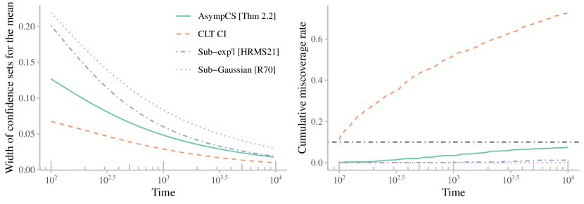
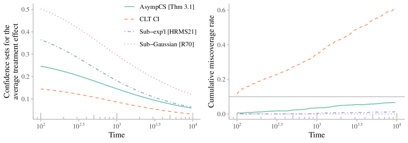
(a) Estimating the mean of bounded random variables (b) Estimating the ATE in a completely randomized Bernoulli experiment (c) Estimating the ATE in an experiment with personalized randomization

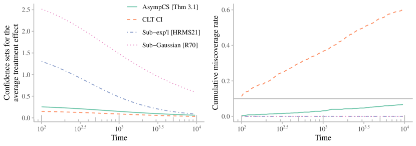
Figure 7: A comparison of $(1-\alpha)\equiv 90$% confidence sets for parameters in three simulation scenarios: (a) mean estimation of bounded random variables, (b) ATE estimation from a completely randomized Bernoulli experiment, and (c) ATE estimation from an experiment with covariate-dependent (“personalized”) randomization. Empirical widths and miscoverage rates were computed with $1000$ replications beginning at time $100$ for mean estimation (Simulation (a)) and time $500$ for ATE estimation (Simulations (b) and (c)). Notice that in all three scenarios, only CSs have miscoverage rates below $\alpha$, but AsympCSs are the only ones that appear to sharply approach this level.

1. The first simulation focuses on estimating the mean $\mu$ of iid Uniform(0, 1) random variables only using knowledge of $[0,1]$-boundedness. For this setting, boundedness allows the CSs of Robbins [41] and Howard et al. [19] to be immediately applicable.

2. The second considers average treatment effect estimation in a randomized experiment with $\{0,1\}$-valued outcomes where everyone is randomly assigned to treatment or control with probability $1/2$. Since all propensity scores are equal to $1/2$, we have that estimates of the influence functions in (42) from Section 3.2 are bounded in $[-2,2]$, and hence the techniques of Robbins [41] and Howard et al. [19] are applicable (as suggested by Howard et al. [19, §4.2]).

3. The third and final simulation considers a similar setup to (b) with the key difference that propensity scores are now covariate-dependent (“personalized”). In this case, as suggested by Howard et al. [19, §4.2], note that estimates of the influence functions (42) lie in $[-1/p_{\mathrm{min}}-1,1/p_{\mathrm{min}}+1]$ where $p_{\mathrm{min}}:=\min\{\operatorname{\mathrm{essinf}}_{x}\pi(x),\operatorname{\mathrm{essinf}}_{x}[1-\pi(x)]\}$, permitting the application of Robbins [41] and Howard et al. [19] as before.

Notice that in all three scenarios, CLT-based CIs have cumulative miscoverage rates that quickly diverge beyond $\alpha=0.1$ while those of CSs — both asymptotic and nonasymptotic — never exceed $\alpha$ before time $10^{4}$. (Note that a longer time horizon of $10^{5}$ is considered only for AsympCSs and CLT-based CIs in Fig. 1, but is omitted here due to the computational expense of Howard et al. [19, Thm 2] at large $t$.) Moreover, notice that nonasymptotic CSs appear to be conservative, while our AsympCSs are much tighter and have miscoverage rates approaching $\alpha$ (as expected in light of Theorem 2.8).

These particular simulation scenarios illustrate situations where AsympCSs are increasingly beneficial over nonasymptotic bounds. First, estimating means of bounded random variables (Fig. 7(a)) is a problem for which several nonasymptotic CIs and CSs exist, and indeed both the bounds of Robbins [41] and especially Howard et al. [19] fare well in this setting. The relatively small variance of Uniform(0, 1) random variables, however, means that asymptotic methods can quickly tighten in this setting while the empirical Bernstein CSs of Howard et al. [19] take a while to adapt to the variance (while those of Robbins [41] never will).

However, AsympCSs are particularly well-suited to the settings of ATE estimation in Figs (b) and (c) where almost-sure bounds on observed random variables can be quite large in comparison to their variances. Fig. 7(b) considers the setting where all propensity scores are equal to $1/2$ which is the “easiest” regime for nonasymptotic methods, meaning the influence function bounds are as tight as possible. Even here, AsympCSs are tighter than the nonasymptotic bounds. On the other hand, Fig. 7(c) considers a setting where propensity scores are highly covariate-dependent, and hence the almost sure bounds on propensity scores $\pi(x)\in[p_{\mathrm{min}},1-p_{\mathrm{min}}]$ must hold for all possible $x$ (in this simulation, $p_{\mathrm{min}}=0.2$). In this setting we see that AsympCSs drastically outperform nonasymptotic CSs without inflating miscoverage rates. Taking this to the logical extreme, it is possible to construct scenarios where $p_{\mathrm{min}}$ is closer and closer to 0, but influence function variances remain bounded. In other words, it is possible to consider scenarios where AsympCSs are arbitrarily tighter than nonasymptotic CSs, without inflating miscoverage rates.

Finally, we remark that while AsympCSs demonstrate substantial benefits over nonasymptotic CSs in terms of tightness, we wish to also highlight their benefits of versatility, and in particular, note that there are many settings for which no simulations could be run since AsympCSs provide the first time-uniform solution in the literature. For example, as a consequence of Bahadur and Savage [1], it is impossible to derive nonasymptotic CSs (or CIs) for the mean of random variables without prior bounds on their moments. By contrast, AsympCSs can handle mean estimation under finite (but unknown) moment assumptions. It is also impossible to derive nonasymptotic CS (and CIs) for the ATE from observational studies (without substantial and unrealistic knowledge of nuisance function estimation errors) but Section 3.3 outlines the first time-uniform solution in the literature. In both of these settings, we cannot run simulations akin to Fig. 7 since there are no prior CSs to compare to.

5 Real data application: effects of IV fluid caps in sepsis patients

Let us now illustrate the use of Theorem 3.2 by sequentially estimating the effect of fluid-restrictive strategies on mortality in an observational study of real sepsis patients. We will use data from the Medical Information Mart for Intensive Care III (MIMIC-III), a freely available database consisting of health records associated with more than 45,000 critical care patients at the Beth Israel Deaconess Medical Center [23, 37]. The data are rich, containing demographics, vital signs, medications, and mortality, among other information collected over the span of 11 years.

Following Shahn et al. [47], we aim to estimate the effect of restricting intravenous (IV) fluids within 24 hours of intensive care unit (ICU) admission on 30-day mortality in sepsis patients. In particular, we considered patients at least 16 years of age satisfying the Sepsis-3 definition — i.e. those with a suspected infection and a Sequential Organ Failure Assessment (SOFA) score of at least 2 [48]. Sepsis-3 patients can be obtained from MIMIC-III using SQL scripts provided by Johnson and Pollard [22], but we provide detailed instructions for reproducing our data collection and analysis process on GitHub. This resulted in a total of 5231 sepsis patients, each of whom received out-of-hospital followup of at least 90 days.

We considered IV fluid intake within 24 hours of ICU admission $\mathscr{L}^{\mathrm{24h}}$. To construct a binary treatment $A\in\{0,1\}$, we dichotomized $\mathscr{L}^{\mathrm{24h}}$ so that $A_{i}=\operatorname{\mathds{1}}(\mathscr{L}^{\mathrm{24h}}_{i}\leq 6\mathrm{L})$. The 30-day mortality $Y$ was defined as 1 if the patient died within 30 days of hospital admission, and 0 otherwise. Baseline covariates $X$ included for modelling consisted of the patients’ age and sex, whether they are diabetic, modified Elixhauser scores [61], and SOFA scores. We are interested in the causal estimand,

$$\psi:=\mathbb{P}\left(Y^{\mathscr{L}^{\mathrm{24h}}\leq 6L}=1\right)-\mathbb{P}\left(Y^{\mathscr{L}^{\mathrm{24h}}>6L}=1\right),$$ (54)

which is the difference in average 30-day mortality that would be observed if all sepsis patients were randomly assigned an IV fluid level according to the lower truncated distribution $\mathbb{P}(\mathscr{L}^{\mathrm{24h}}\leq l\mid\mathscr{L}^{\mathrm{24h}}\leq 6\mathrm{L})$ versus the upper truncated distribution $\mathbb{P}(\mathscr{L}^{\mathrm{24h}}\leq l\mid\mathscr{L}^{\mathrm{24h}}>6\mathrm{L})$ [11]. While this is technically a stochastic intervention effect, we have that under the same causal identification assumptions discussed in Section 3, $\psi$ is identified as

$$\psi=\mathbb{E}\left\{\mathbb{E}(Y\mid X,A=1)-\mathbb{E}(Y\mid X,A=0)\right\},$$ (55)

which is the same functional considered in the previous sections. Therefore, we can estimate $\psi$ under the same assumptions and with the same techniques as Section 3.3. Similar to the simulated data analysis of Fig. 4 and Fig. 5, we produced AsympCSs for $\psi$ using difference-in-means, parametric AIPW, and stacking-based AIPW estimators to demonstrate the impacts of different modeling choices on estimation (see Fig. 8).

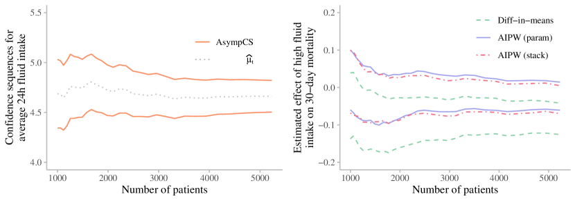
Figure 8: Left-hand side: a $90\%$ AsympCS used to track the average 24h fluid intake over time. Right-hand side: Three 90%-AsympCSs for the causal effect of capped IV fluid intake (defined as $\leq 6$ litres) on 30-day mortality using the same three estimators as those outlined in Fig. 5. Notice that an analysis using a difference-in-means estimator would conclude that the treatment effect is negative after observing fewer than 1500 patients.

Remark 4.

These simple binary treatment and outcome variables were used for simplicity so that the methods outlined in Section 3.3 are immediately applicable, but as discussed in Section 3.5, our AsympCSs may be used to sequentially estimate other causal functionals.

Our stacking-based AIPW AsympCSs cover the null treatment effect of 0 from the $1000^{\text{th}}$ to the $5231^{\text{st}}$ observed patient, and thus we cannot conclude with confidence whether 6L IV fluid caps have an effect on 30-day mortality in sepsis patients. Interestingly, the width and center of AsympCSs based on both stacking and parametric estimators are roughly equal, which is in contrast to the simulations provided in the previous sections. This could be due to the fact that the true regression or propensity score functions lie in the parametric models considered by “AIPW (param)” or because they are good approximations. Since this analysis is not a simulation, we cannot know with certainty one way or another. Nevertheless, because our stacked estimator uses the parametric (linear and logistic regression) models as candidate predictors, the stacking-based AsympCS is guaranteed to asymptotically match the parametric one if the parametric models are correctly specified. As such, there is little reason to use the parametric AIPW AsympCS alone.

Note that these stacking-based AsympCSs nearly drop below 0 after observing the $5231^{\text{st}}$ patient’s outcome. If we were using fixed-time confidence intervals, we would need to resist the temptation to resume data collection (e.g. to see whether the null hypothesis $H_{0}:\psi=0$ could be rejected with a slightly larger sample size) as this would inflate type-I error rates (as seen in Fig. 1). On the other hand, our AsympCSs permit exactly this form of continued sampling.

6 Conclusion

This paper introduced the notion of an “asymptotic confidence sequence” as the time-uniform analogue of an asymptotic confidence interval based on the central limit theorem. We derived an explicit universal asymptotic confidence sequence for the mean from iid observations under weak moment assumptions by appealing to the strong invariance principle of Strassen [50]. These results were extended to the setting where observations’ distributions (including means and variances) can vary over time under martingale dependence, such that our confidence sequences capture a moving parameter — the running average of the conditional means so far. We then applied the aforementioned results to the problem of doubly robust sequential inference for the average treatment effect in both randomized experiments and observational studies under iid sampling. Finally, we showed how these causal applications remain valid in the non-iid setting where distributions change over time, in which case our confidence sequences capture a running average of individual treatment effects. The aforementioned results will enable researchers to continuously monitor sequential experiments — such as clinical trials and online A/B tests — as well as sequential observational studies even if treatment effects do not remain stationary over time.

Acknowledgements

IW-S thanks Tudor Manole for early conversations regarding strong approximation theory. AR acknowledges funding from NSF Grant DMS1916320, NSF Grant DMS2053804, an Adobe faculty research award, and an NSF DMS (CAREER) 1945266. EK gratefully acknowledges support from NSF Grant DMS1810979. The authors thank Ziyu (Neil) Xu, Dae Woong Ham, Eric J. Tchetgen Tchetgen, and the CMU causal inference working group for helpful discussions.

Appendix A Proofs of the main results

A.1 Proof of Theorem 2.2

We first introduce a lemma that will later be used in the main proof.

Lemma A.1 (Strong Gaussian approximation of the sample average).

Let $(Y_{t})_{t=1}^{\infty}$ be an iid sequence of random variables with mean $\mu$, variance $\sigma^{2}$, and let $\widehat{\sigma}_{t}^{2}$ be the sample variance. Then (after sufficiently enriching the probability space), there exist iid Gaussian random variables $(G_{t})_{t=1}^{\infty}$ such that

$$\frac{1}{t}\sum_{i=1}^{t}(Y_{i}-\mu)=\frac{\widehat{\sigma}_{t}}{t}\sum_{i=1}^{t}G_{i}+\varepsilon_{t}$$

where $\varepsilon_{t}=o(\sqrt{\log\log t/t})$. One could also replace $\sum_{i=1}^{t}G_{i}$ with a Wiener process $(W_{t})_{t\geq 0}$.

Proof.

By the strong approximation theorem of Strassen [50], we have that (after sufficiently enriching the probability space) there exist iid Gaussian random variables $(G_{t})_{{t}={1}}^{\infty}$ such that

$$\frac{1}{t}\sum_{i=1}^{t}(Y_{i}-\mu)=\frac{\sigma}{t}\sum_{i=1}^{t}G_{i}+\kappa_{t}$$ (56)

with $\kappa_{t}=o(\sqrt{\log\log t/t})$. Since $(G_{t})_{t=1}^{\infty}$ have mean zero and unit variance, we have by the LIL that

$$\frac{1}{t}\sum_{i=1}^{t}G_{i}=O\left(\sqrt{\frac{\log\log t}{t}}\right).$$ (57)

Now, by the strong law of large numbers, $\widehat{\sigma}_{t}\xrightarrow{a.s.}\sigma$. Combining this fact with with (56), we have

$$\frac{1}{t}\sum_{i=1}^{t}(Y_{i}-\mu) =\frac{\widehat{\sigma}_{t}+o(\widetilde{\sigma}_{t}^{2})}{t}\sum_{i=1}^{t}G_{i}+\kappa_{t}$$

$$=\frac{\widehat{\sigma}_{t}}{t}\sum_{i=1}^{t}G_{i}+\kappa_{t}+o\left(\sqrt{\frac{\log\log t}{t}}\right)$$

$$=\frac{\widehat{\sigma}_{t}}{t}\sum_{i=1}^{t}G_{i}+o\left(\sqrt{\frac{\log\log t}{t}}\right),$$

which completes the proof. ∎

Proof of Theorem 2.2.

The proof proceeds in 3 steps. First, we use the fact that for any martingale $M_{t}(\lambda)$, we have that $\int_{\mathbb{R}}M_{t}(\lambda)dF(\lambda)$ is also a martingale where $F$ is any probability distribution on $\mathbb{R}$ [18, 19]. We apply this fact to an exponential Gaussian martingale and use a Gaussian density $f(\lambda;0,\rho^{2})$ as the mixing distribution. Second, we apply Ville’s inequality [62] to this mixture exponential Gaussian martingale to obtain Robbins’ normal mixture confidence sequence [41]. Third, we use Lemma A.1 to approximate $\sum_{i=1}^{t}(Y_{i}-\mu)$ by a cumulative sum of Gaussian random variables and apply the results from steps 1 and 2.

Step 1

Let $(W_{t})_{t\geq 0}$ be a Wiener process and write the exponential process for any $\lambda\in\mathbb{R}$,

$$M_{t}(\lambda):=\exp\left\{\lambda W_{t}-t\lambda^{2}/2\right\}.$$

It is well-known that $M_{t}(\lambda)$ is a nonnegative martingale starting at $M_{0}\equiv 1$ with respect to the Brownian filtration. By Fubini’s theorem, for any probability distribution $F(\lambda)$ on $\mathbb{R}$, we also have that the mixture,

$$\int_{\lambda\in\mathbb{R}}M_{t}(\lambda)dF(\lambda)$$

is a nonnegative martingale with initial value one with respect to the same filtration [41]. In particular, consider the Gaussian probability distribution function $f(\lambda;0,\rho^{2})$ with mean zero and variance $\rho^{2}>0$ as the mixing distribution. The resulting martingale can be written as

$$M_{t} :=\int_{\lambda\in\mathbb{R}}\exp\left\{\lambda W_{t}-\frac{t\lambda^{2}}{2}\right\}f(\lambda;0,\rho^{2})d\lambda$$

$$=\frac{1}{\sqrt{2\pi\rho^{2}}}\int_{\lambda}\exp\left\{\lambda W_{t}-\frac{t\lambda^{2}}{2}\right\}\exp\left\{\frac{-\lambda^{2}}{2\rho^{2}}\right\}d\lambda$$

$$=\frac{1}{\sqrt{2\pi\rho^{2}}}\int_{\lambda}\exp\left\{\lambda W_{t}-\frac{\lambda^{2}(t\rho^{2}+1)}{2\rho^{2}}\right\}d\lambda$$

$$=\frac{1}{\sqrt{2\pi\rho^{2}}}\int_{\lambda}\exp\left\{\frac{-\lambda^{2}(t\rho^{2}+1)+2\lambda\rho^{2}W_{t}}{2\rho^{2}}\right\}d\lambda$$

$$=\frac{1}{\sqrt{2\pi\rho^{2}}}\int_{\lambda}\exp\left\{\frac{-a(\lambda^{2}-\frac{b}{a}2\lambda)}{2\rho^{2}}\right\}d\lambda$$

by setting $a:=t\rho^{2}+1$ and $b:=\rho^{2}W_{t}$. Focusing on the integrand and completing the square, we have

$$\exp\left\{\frac{-\lambda^{2}+2\lambda\frac{b}{a}+\left(\frac{b}{a}\right)^{2}-\left(\frac{b}{a}\right)^{2}}{2\rho^{2}/a}\right\} =\exp\left\{\frac{-(\lambda-b/a)^{2}}{2\rho^{2}/a}+\frac{a\left(b/a\right)^{2}}{2\rho^{2}}\right\}$$

$$=\underbrace{\exp\left\{\frac{-(\lambda-b/a)^{2}}{2\rho^{2}/a}\right\}}_{\propto f(\lambda,b/a,\rho^{2}/a)}\exp\left\{\frac{b^{2}}{2a\rho^{2}}\right\}.$$

Plugging this back into the integral and multiplying the entire quantity by $\frac{a^{-1/2}}{a^{-1/2}}$, we finally get the closed-form expression of the mixture exponential Wiener process,

$$M_{t} :=\underbrace{\frac{1}{\sqrt{2\pi\rho^{2}/a}}\int_{\lambda\in\mathbb{R}}\exp\left\{\frac{-(\lambda-b/a)^{2}}{2\rho^{2}/a}\right\}d\lambda}_{=1}\frac{\exp\left\{\frac{b^{2}}{2a\rho^{2}}\right\}}{\sqrt{a}}$$

$$=\frac{\exp\left\{\frac{\rho^{2}W_{t}^{2}}{2(t\rho^{2}+1)}\right\}}{\sqrt{t\rho^{2}+1}}.$$ (58)

Step 2

Since $M_{t}$ is a nonnegative martingale with initial value one, we have by Ville’s inequality [62] that

$$\mathbb{P}(\forall t\geq 1,\ M_{t}<1/\alpha)\geq 1-\alpha.$$

Writing this out explicitly for $M_{t}$ and solving for $W_{t}$ algebraically, we have that

$$\mathbb{P}\left(\forall t\geq 1,\ \frac{\rho^{2}W_{t}^{2}}{2(t\rho^{2}+1)}<\log(1/\alpha)+\log\left(\sqrt{t\rho^{2}+1}\right)\right)$$

$$=\ \mathbb{P}\left(\forall t\geq 1,\ \left|W_{t}/t\right|<\sqrt{\frac{2(t\rho^{2}+1)}{t^{2}\rho^{2}}\log\left(\frac{\sqrt{t\rho^{2}+1}}{\alpha}\right)}\right)\geq 1-\alpha.$$

Step 3

First, note that by the triangle inequality,

$$\left|\frac{1}{t}\sum_{i=1}^{t}Y_{i}-\mu\right|\leq\left|\frac{1}{t}\sum_{i=1}^{t}(Y_{i}-\mu)-\frac{\widehat{\sigma}_{t}}{t}W_{t}\right|+\widehat{\sigma}_{t}\left|W_{t}\right|,$$

and thus by Lemma A.1 and Step 2, we have with probability at least $(1-\alpha)$,

$$\forall t\geq 1,\ \left|\frac{1}{t}\sum_{i=1}^{t}Y_{i}-\mu\right|<\underbrace{\widehat{\sigma}_{t}\sqrt{\frac{2(t\rho^{2}+1)}{t^{2}\rho^{2}}\log\left(\frac{\sqrt{t\rho^{2}+1}}{\alpha}\right)}}_{\widebar{\mathfrak{B}}_{t}^{\mathcal{G}}}+\varepsilon_{t}$$

where $\varepsilon_{t}$ is defined as in Lemma A.1. Finally, note that

$$\frac{\widebar{\mathfrak{B}}_{t}^{\mathcal{G}}+\varepsilon_{t}}{\widebar{\mathfrak{B}}_{t}^{\mathcal{G}}}\xrightarrow{\mathrm{a.s.}}1,$$ (59)

completing the proof. ∎

A.2 Proof of Lemma 2.4

Proof.

Take $L_{t}^{\star}:=L_{t}-(\widehat{\theta}_{t}-\theta_{t}-Z_{t})$ and $U_{t}^{\star}:=U_{t}-(\widehat{\theta}_{t}-\theta_{t}-Z_{t})$.

$$\mathbb{P}\left(\forall t\in\mathcal{T},\ \theta_{t}\in\left[\widehat{\theta}_{t}+L_{t}^{\star},\widehat{\theta}_{t}+U_{t}^{\star}\right]\right)$$ (60)

$$=\ \mathbb{P}\left(\forall t\in\mathcal{T},\ \theta_{t}\in\left[\widehat{\theta}_{t}+L_{t}-(\widehat{\theta}_{t}-\theta_{t}-Z_{t}),\widehat{\theta}_{t}+U_{t}-(\widehat{\theta}_{t}-\theta_{t}-Z_{t})\right]\right)$$ (61)

$$=\ \mathbb{P}\left(\forall t\in\mathcal{T},\ Z_{t}\in\left[L_{t},U_{t}\right]\right)\geq 1-\alpha,$$ (62)

where the last line follows from G-2, and hence we have shown Eq. 18. It remains to show that $L_{t}^{\star}/\widehat{L}_{t}\xrightarrow{\mathrm{a.s.}}1$ and $U_{t}^{\star}/\widehat{U}_{t}\xrightarrow{\mathrm{a.s.}}1$. Indeed,

$$L_{t}^{\star}/\widehat{L}_{t} =(L_{t}^{\star}/L_{t})\cdot\underbrace{(L_{t}/\widehat{L}_{t})}_{=1+o(1)}$$ (63)

$$=\left(\frac{L_{t}-(\widehat{\theta}_{t}-\theta_{t}-Z_{t})}{L_{t}}\right)\cdot(1+o(1))$$ (64)

$$=\left(\frac{L_{t}-o(r_{t})}{L_{t}}\right)\cdot(1+o(1))$$ (65)

$$=\left(1+o(1)\right)\cdot(1+o(1))\xrightarrow{\mathrm{a.s.}}1,$$ (66)

where (64) follows from the definition of $L_{t}^{\star}$ and G-4, (65) follows from G-1, and (66) follows from G-3. By a similar argument, $U_{t}^{\star}/\widehat{U}_{t}\xrightarrow{\mathrm{a.s.}}1$, completing the proof. ∎

A.3 Proof of Theorem 2.5

First, we present a lemma that is implicit in the proof of Strassen [51, Theorem 4.4] and which will be central to the proof of Theorem 2.5.

Lemma A.2 (Strong approximation under martingale dependence).

Let $(Y_{t})_{t=1}^{\infty}$ be a sequence of random variables with conditional means and variances given by $\mu_{t}=\mathbb{E}(Y_{t}\mid Y_{1}^{t-1})$ and $\sigma_{t}^{2}=\operatorname{\mathrm{var}}(Y_{t}\mid Y_{1}^{t-1})$, respectively. Let $V_{t}=\sum_{i=1}^{t}\sigma_{i}^{2}$ be the cumulative conditional variance process, and suppose that $V_{t}\to\infty$ almost surely. Furthermore, assume that the Lindeberg-type condition given in L-2 holds. Then, on a potentially enriched probability space, there exist iid standard Gaussians $(G_{t})_{t=1}^{\infty}$ such that

$$\frac{1}{t}\sum_{i=1}^{t}(Y_{i}-\mu_{i})-\frac{1}{t}\sum_{i=1}^{t}\sigma_{i}G_{i}=o\left(\frac{V_{t}^{3/8}\log V_{t}}{t}\right).$$ (67)

Proof of Lemma A.2.

The proof centrally relies on Strassen [51, Eq. 159] which states that on a potentially enriched probability space,

$$\sum_{i=1}^{t}(Y_{i}-\mu_{i})=\xi(V_{t})+o(h(V_{t}))$$ (68)

where $\xi$ is a standard Brownian motion, and $h(v)=(vf(v))^{1/4}\log v$ for some $f(\cdot)$ so that $f(v)$ is increasing in $v$, but $f(v)/v$ is decreasing. For the purposes of this proof, we set $f(v)=v^{1/2}$, and hence $h(v)=v^{3/8}\log v$. Since a standard Brownian motion evaluated at $V_{t}=\sum_{i=1}^{t}\sigma_{i}^{2}$ is equal in distribution to the discrete time process $\sum_{i=1}^{t}\sigma_{i}G_{i}$ at each $t$, we have that

$$\sum_{i=1}^{t}(Y_{i}-\mu_{i})=\sum_{i=1}^{t}\sigma_{i}G_{i}+o\left(V_{t}^{3/8}\log V_{t}\right),$$ (69)

which completes the proof after dividing both sides by $t$. ∎

With Lemma A.2 in mind, we can now prove the main result (Theorem 2.5).

Proof of Theorem 2.5.

The proof proceeds in four steps, each step being dedicated to satisfying one of Lemma 2.4’s conditions (G-1–G-4). Step 1 follows quickly from Lemma A.2, while Step 2 requires us to derive a (sub)-Gaussian boundary for non-iid observations under martingale dependence (which appears to be new, to the best of our knowledge). Step 3 follows from the arguments in Steps 1 and 2, and Step 4 follows from a simple argument that uses L-3.

Step 1: Satisfying G-1 via Strassen [51] and Sections L-1 and L-2

Notice that the assumptions of Lemma A.2 are satisfied by Sections L-1 and L-2, and hence G-1 follows using the approximating process formed by $\frac{1}{t}\sum_{i=1}^{t}\sigma_{i}G_{i}$ as in Lemma A.2 with a rate of $r_{t}:=t^{-1}V_{t}^{3/8}\log V_{t}$. That is,

$$\left(\widehat{\mu}_{t}-\widetilde{\mu}_{t}\right)-\frac{1}{t}\sum_{i=1}^{t}\sigma_{i}G_{i}=\frac{V_{t}^{3/8}\log V_{t}}{t}.$$ (70)

In Step 2, we provide a nonasymptotic boundary for the process given by $\frac{1}{t}\sum_{i=1}^{t}\sigma_{i}G_{i}$.

Step 2: Satisfying G-2 using a nonasymptotic sub-Gaussian boundary

Let $\sigma_{i}G_{i}$ be as in Lemma A.2. Define the conditional variance $\sigma_{t}^{2}:=\operatorname{\mathrm{var}}(Y_{t}\mid Y_{1}^{t-1})$ and note that

$$\widetilde{M}_{t}(\lambda):=\exp\left\{\sum_{i=1}^{t}(\lambda\sigma_{i}G_{i}-\lambda^{2}\sigma_{i}^{2}/2)\right\}$$

is a nonnegative martingale starting at one (with respect to the filtration generated by $(G_{t},\sigma_{t})_{t=1}^{\infty}$). Mixing over $\lambda$ with the probability density $dF(\lambda)$ of a mean-zero Gaussian with variance $\rho^{2}$ as in the proof of Theorem 2.2, we have that

$$\widetilde{M}_{t}:=\int_{\lambda\in\mathbb{R}}\widetilde{M}_{t}(\lambda)dF(\lambda)=\exp\left\{\frac{\rho^{2}(\sum_{i=1}^{t}\sigma_{i}G_{i})^{2}}{2(V_{t}\rho^{2}+1)}\right\}\cdot\left(V_{t}\rho^{2}+1\right)^{-1/2}$$

is also a martingale. By Ville’s inequality for nonnegative (super)martingales, we have that $\mathbb{P}(\exists t:\widetilde{M}_{t}\geq 1/\alpha)\leq\alpha$ and hence with probability at least $(1-\alpha)$,

$$\forall t\geq 1,\ \left|\frac{1}{t}\sum_{i=1}^{t}\sigma_{i}G_{i}\right|<\sqrt{\frac{2(V_{t}\rho^{2}+1)}{t^{2}\rho^{2}}\log\left(\frac{\sqrt{V_{t}\rho^{2}+1}}{\alpha}\right)}.$$ (71)

In particular, combined with Step 1, we have that

$$\left(\widehat{\mu}_{t}\pm\sqrt{\frac{2(V_{t}\rho^{2}+1)}{t^{2}\rho^{2}}\log\left(\frac{\sqrt{V_{t}\rho^{2}+1}}{\alpha}\right)}\right)$$ (72)

forms a $(1-\alpha)$-AsympCS for $\widetilde{\mu}_{t}$.

Step 3: Satisfying G-3 as a consequence of Sections G-1 and G-2

Inspecting the boundary in (71), we notice that $V_{t}^{3/8}\log V_{t}/t=o(\sqrt{V_{t}\log V_{t}}/t)$ and hence G-3 is satisfied.

Step 4: Satisfying G-4 via L-3

Writing out the margin of (72) combined with L-3: $\widehat{\sigma}_{t}^{2}-\widetilde{\sigma}_{t}^{2}=o(\widetilde{\sigma}_{t}^{2})$ and recalling that $V_{t}:=t\widetilde{\sigma}_{t}$, we have

$$\sqrt{\frac{2(V_{t}\rho^{2}+1)}{t^{2}\rho^{2}}\log\left(\frac{\sqrt{V_{t}\rho^{2}+1}}{\alpha}\right)} =\sqrt{\frac{2(t(\widehat{\sigma}_{t}^{2}+o(\widetilde{\sigma}_{t}^{2}))\rho^{2}+1)}{t^{2}\rho^{2}}\log\left(\frac{\sqrt{t(\widehat{\sigma}_{t}^{2}+o(\widetilde{\sigma}_{t}^{2})\rho^{2}+1}}{\alpha}\right)}$$

$$=\sqrt{\frac{t(\widehat{\sigma}_{t}^{2}+o(\widetilde{\sigma}_{t}^{2})\rho^{2}+1}{t^{2}\rho^{2}}\log\left(\frac{t(\widehat{\sigma}_{t}^{2}+o(\widetilde{\sigma}_{t}^{2})\rho^{2}+1}{\alpha^{2}}\right)}$$

$$=\sqrt{\frac{t\widehat{\sigma}_{t}^{2}\rho^{2}+o(t\widetilde{\sigma}_{t}^{2})+1}{t^{2}\rho^{2}}\log\left(\frac{t\widehat{\sigma}_{t}^{2}\rho^{2}+o(t\widetilde{\sigma}_{t}^{2})+1}{\alpha^{2}}\right)}$$

$$=\sqrt{\left(\frac{t\widehat{\sigma}_{t}^{2}\rho^{2}+1}{t^{2}\rho^{2}}+o(\widetilde{\sigma}_{t}^{2}/t)\right)\log\left(\frac{t\widehat{\sigma}_{t}^{2}\rho^{2}+o(t\widetilde{\sigma}_{t}^{2})+1}{\alpha^{2}}\right)}.$$ (73)

Focusing on the logarithmic factor, we have

$$\log\left(\frac{t\widehat{\sigma}_{t}^{2}\rho^{2}+o(t\widetilde{\sigma}_{t}^{2})+1}{\alpha^{2}}\right) =\log\left(\frac{1+t\widehat{\sigma}^{2}_{t}\rho^{2}}{\alpha^{2}}+o(t\widetilde{\sigma}_{t}^{2})\right)$$

$$=\log\left(\frac{1+t\widehat{\sigma}^{2}_{t}\rho^{2}}{\alpha^{2}}\left[1+o\left(1\right)\right]\right)$$

$$=\log\left(\frac{1+t\widehat{\sigma}_{t}^{2}\rho^{2}}{\alpha^{2}}\right)+\log\left(1+o\left(1\right)\right)$$

$$=\log\left(\frac{1+t\widehat{\sigma}_{t}^{2}\rho^{2}}{\alpha^{2}}\right)+o\left(1\right)$$ (74)

where the last line follows from the Taylor expansion $\log(1+x)=x+o(1)$ for $|x|<1$. Combining (73) and (74), we have that the margin of (72) can be written as

$$\sqrt{\frac{2(V_{t}\rho^{2}+1)}{t^{2}\rho^{2}}\log\left(\frac{\sqrt{V_{t}\rho^{2}+1}}{\alpha}\right)} =\sqrt{\left(\frac{t\widehat{\sigma}_{t}^{2}\rho^{2}+1}{t^{2}\rho^{2}}+o(V_{t}/t^{2})\right)\left[\log\left(\frac{1+t\widehat{\sigma}_{t}^{2}\rho^{2}}{\alpha^{2}}\right)+o(1)\right]}$$

$$=\sqrt{\frac{t\widehat{\sigma}_{t}^{2}\rho^{2}+1}{t^{2}\rho^{2}}\log\left(\frac{1+t\widehat{\sigma}_{t}^{2}\rho^{2}}{\alpha^{2}}\right)+o(V_{t}/t^{2})+o(V_{t}\log V_{t}/t^{2})+o(V_{t}/t^{2})}$$

$$=\sqrt{\frac{2(t\widehat{\sigma}_{t}^{2}\rho^{2}+1)}{t^{2}\rho^{2}}\log\left(\frac{\sqrt{1+t\widehat{\sigma}_{t}^{2}\rho^{2}}}{\alpha}\right)+o(V_{t}\log V_{t}/t^{2})}$$

$$\leq\sqrt{\frac{2(t\widehat{\sigma}_{t}^{2}\rho^{2}+1)}{t^{2}\rho^{2}}\log\left(\frac{\sqrt{1+t\widehat{\sigma}_{t}^{2}\rho^{2}}}{\alpha}\right)}+o\left(\frac{\sqrt{V_{t}\log V_{t}}}{t}\right),$$ (75)

where the last inequality follows from $\sqrt{a+b}\leq\sqrt{a}+\sqrt{b}$ for $a,b\geq 0$. In particular, letting

$$[L_{t},U_{t}] :=\left[\widehat{\mu}_{t}\pm\sqrt{\frac{2(V_{t}\rho^{2}+1)}{t^{2}\rho^{2}}\log\left(\frac{\sqrt{V_{t}\rho^{2}+1}}{\alpha}\right)}\right]$$ (76)

$$\text{and}\quad[\widehat{L}_{t},\widehat{U}_{t}] :=\left[\widehat{\mu}_{t}\pm\sqrt{\frac{2(t\widehat{\sigma}_{t}^{2}\rho^{2}+1)}{t^{2}\rho^{2}}\log\left(\frac{\sqrt{t\widehat{\sigma}_{t}^{2}\rho^{2}+1}}{\alpha}\right)}\right],$$ (77)

we have that $\widehat{L}_{t}/L_{t}\xrightarrow{\mathrm{a.s.}}1$ and $\widehat{U}_{t}/U_{t}\xrightarrow{\mathrm{a.s.}}1$, satisfying G-4 and completing the proof of Theorem 2.5.

∎

A.4 Proof of Corollary 2.6

Proof.

As alluded to in the paragraph following Corollary 2.6, it suffices to show that if the following regularity conditions hold, i.e.

$$\sum_{i=1}^{\infty}\frac{\mathbb{E}|Y_{i}^{2}-\mathbb{E}Y_{i}^{2}|^{1+\beta}}{V_{i}^{1+\beta}}<\infty,\quad\widetilde{\mu}_{t}^{2}=o(V_{t}),\quad\text{and}\quad\frac{1}{t}\sum_{i=1}^{t}(\mu_{i}-\widetilde{\mu}_{t})^{2}=o(\widetilde{\sigma}_{t}^{2}),$$ (78)

then L-3 is satisfied, meaning $\widehat{\sigma}_{t}^{2}/\widetilde{\sigma}_{t}^{2}\xrightarrow{\mathrm{a.s.}}1$ where $\widehat{\sigma}_{t}^{2}:=\frac{1}{t}\sum_{i=1}^{t}Y_{i}^{2}-\left(\frac{1}{t}\sum_{i=1}^{t}Y_{i}\right)^{2}$. To this end, notice that by Petrov [35, Theorem 12], we have that the left-most inequality of (78) implies that

$$\frac{1}{t}\sum_{i=1}^{t}\left[Y_{i}^{2}-\mathbb{E}(Y_{i}^{2})\right]=o(\widetilde{\sigma}_{t}^{2}).$$ (79)

Writing out the difference $\widehat{\sigma}_{t}^{2}-\widetilde{\sigma}_{t}^{2}$, we see that

$$\widehat{\sigma}_{t}^{2}-\widetilde{\sigma}_{t}^{2} \equiv\frac{1}{t}\sum_{i=1}^{t}Y_{i}^{2}-\left(\frac{1}{t}\sum_{i=1}^{t}Y_{i}\right)^{2}-\frac{1}{t}\sum_{i=1}^{t}\left[\mathbb{E}(Y_{i}^{2})-(\mathbb{E}Y_{i})^{2}\right]$$ (80)

$$=\underbrace{\frac{1}{t}\sum_{i=1}^{t}\left[Y_{i}^{2}-\mathbb{E}(Y_{i}^{2})\right]}_{=o(\widetilde{\sigma}_{t}^{2})\text{ by }\eqref{eq:lyapunov-proof-second-moment-estimation}}-\underbrace{\left[\left(\frac{1}{t}\sum_{i=1}^{t}Y_{i}\right)^{2}-\frac{1}{t}\sum_{i=1}^{t}(\mathbb{E}Y_{i})^{2}\right]}_{(\star)}.$$ (81)

Focusing now only $(\star)$, we use the Lyapunov-type condition assumption $\sum_{i=1}^{\infty}\frac{\mathbb{E}|Y_{i}-\mu_{i}|^{2+\delta}}{\sqrt{V_{i}}^{2+\delta}}<\infty$ combined with Petrov [35, Theorem 12] to note that $\frac{1}{t}\sum_{i=1}^{t}(Y_{i}-\mu_{i})=o(\sqrt{V_{t}}/t)$ and hence

$$(\star) \equiv\left(\widetilde{\mu}_{t}+o(\sqrt{V_{t}}/t)\right)^{2}-\frac{1}{t}\sum_{i=1}^{t}(\mathbb{E}Y_{i})^{2}$$ (82)

$$=\widetilde{\mu}_{t}^{2}+o(\widetilde{\mu}_{t}\sqrt{V_{t}}/t)+o(V_{t}/t^{2})-\frac{1}{t}\sum_{i=1}^{t}(\mathbb{E}Y_{i})^{2}$$ (83)

$$=\left(\frac{1}{t}\sum_{i=1}^{t}\mu_{i}\right)^{2}+o(\widetilde{\mu}_{t}\sqrt{V_{t}}/t)+o(V_{t}/t^{2})-\frac{1}{t}\sum_{i=1}^{t}(\mathbb{E}Y_{i})^{2}$$ (84)

$$=-\frac{1}{t}\sum_{i=1}^{t}\left(\mu_{i}-\widetilde{\mu}_{t}\right)^{2}+o(\widetilde{\mu}_{t}\sqrt{V_{t}}/t)+o(V_{t}/t^{2})$$ (85)

$$=o(\widetilde{\sigma}_{t}^{2}),$$ (86)

where the final line follows from the assumptions of (78). This completes the proof of Corollary 2.6.

∎

A.5 Proof of Theorems 3.1 and 3.2

In the proofs that follow, we will make extensive use of some convenient notation, namely the sample average operator $\mathbb{P}_{t}f(Z)\equiv\frac{1}{t}\sum_{i=1}^{t}f(Z_{i})$ and the conditional expectation operator $\mathbb{P}\widehat{f}(Z)\equiv\mathbb{P}(\widehat{f}(Z_{i})\mid Z_{1}^{\prime},\dots,Z_{n}^{\prime})$ where $Z_{1}^{\prime},\dots,Z_{n}^{\prime}$ are the data used to construct $\widehat{f}$.

First, let us analyze the almost-sure behavior of the AIPW estimator $\widehat{\psi}_{t}$ for the average treatment effect $\psi$.

Lemma A.3 (Decomposition of $\widehat{\psi}_{t}-\psi$).

Let $\widehat{\psi}_{t}:=\mathbb{P}_{T}(\widehat{f}_{{T^{\prime}}})=\frac{1}{{T}}\sum_{i=1}^{T}\widehat{f}_{{T^{\prime}}}(Z_{i}^{\mathrm{eval}})$ be a (possibly misspecified) estimator of $\psi:=\mathbb{P}(f)=\mathbb{E}\{f(Z^{\mathrm{eval}})\}$ based on $(Z^{\mathrm{eval}}_{1},\dots,Z^{\mathrm{eval}}_{T})$ where $\widehat{f}_{{T^{\prime}}}$ can be any estimator built from $(Z^{\mathrm{trn}}_{1},\dots,Z^{\mathrm{trn}}_{{T^{\prime}}})$ and $f:\mathcal{Z}\rightarrow\mathbb{R}$ any function. Furthermore, assume that there exists $\widebar{f}$ such that $\|\widehat{f}_{{T^{\prime}}}-\widebar{f}\|_{L_{2}(\mathbb{P})}\rightarrow 0$. In other words, $\widehat{f}_{{T^{\prime}}}$ is an estimator of $f$ but may instead converge to $\widebar{f}$. Then we have the decomposition,

$$\widehat{\psi}_{t}-\psi=\Gamma^{\mathrm{SA}}_{t}+\Gamma^{\mathrm{EP}}_{t}+\Gamma^{\mathrm{B}}_{t}$$

where

$$\Gamma^{\mathrm{SA}}_{t} :=\ (\mathbb{P}_{T}-\mathbb{P})\widebar{f}\quad$$ is the centered sample average term,

$$\Gamma^{\mathrm{EP}}_{t} :=\ (\mathbb{P}_{T}-\mathbb{P})(\widehat{f}-\widebar{f})\quad$$ is the empirical process term, and

$$\Gamma^{\mathrm{B}}_{t} :=\ \mathbb{P}(\widehat{f}-f)\quad$$ is the bias term.

Proof.

By definition of the quantities involved, we decompose

$$\widehat{\psi}_{t}-\psi =\mathbb{P}_{T}(\widehat{f}_{{T^{\prime}}})-\mathbb{P}(f)$$

$$=(\mathbb{P}_{T}-\mathbb{P})(\widehat{f}_{{T^{\prime}}})+\mathbb{P}(\widehat{f}_{{T^{\prime}}}-f)$$

$$=\underbrace{(\mathbb{P}_{T}-\mathbb{P})(\widehat{f}_{{T^{\prime}}}-\widebar{f})}_{\Gamma^{\mathrm{EP}}_{t}}+\underbrace{(\mathbb{P}_{T}-\mathbb{P})\widebar{f}}_{\Gamma^{\mathrm{SA}}_{t}}+\underbrace{\mathbb{P}(\widehat{f}_{{T^{\prime}}}-f)}_{\Gamma^{\mathrm{B}}_{t}},$$

which completes the proof. ∎

Now, let us analyze the almost-sure behaviour of the empirical process term $\Gamma^{\mathrm{EP}}_{t}$ and the bias term $\Gamma^{\mathrm{B}}_{t}$ to show that they vanish asymptotically at sufficiently fast rates. First, let us examine $\Gamma^{\mathrm{EP}}_{t}$.

Lemma A.4 (Almost sure convergence of $\Gamma^{\mathrm{EP}}_{t}$).

Let $\mathbb{P}_{T}$ denote the empirical measure over $\mathbf{Z}^{\mathrm{eval}}_{T}:=(Z^{\mathrm{eval}}_{1},\dots,Z_{T}^{\mathrm{eval}})$ and let $\widehat{f}_{{T^{\prime}}}(z)$ be any function estimated from a sample ${\mathcal{D}}^{\mathrm{trn}}_{{T^{\prime}}}=(Z^{\mathrm{trn}}_{1},Z^{\mathrm{trn}}_{2},\dots,Z^{\mathrm{trn}}_{{T^{\prime}}})$ which is independent of ${\mathcal{D}}^{\mathrm{eval}}_{T}$. If $\widehat{\pi}_{t}\in[\delta,1-\delta]$ almost surely, then,

$$\Gamma^{\mathrm{EP}}_{t}:=(\mathbb{P}_{T}-\mathbb{P})(\widehat{f}_{{T^{\prime}}}-\widebar{f})=O\left(\left\{\sum_{a=0}^{1}\|\widehat{\mu}^{a}_{t}-\widebar{\mu}^{a}\|_{L_{2}(\mathbb{P})}\right\}\sqrt{\frac{\log\log t}{t}}\right).$$

In particular, if $\|\widehat{\mu}^{a}_{t}-\widebar{\mu}^{a}\|_{L_{2}(\mathbb{P})}=o(1)$ for each $a$, then we have that $\Gamma^{\mathrm{EP}}_{t}$ almost-surely converges to 0 at a rate of $o(\sqrt{\log\log t/t})$, but possibly faster.

The proof proceeds in two steps. First, we use an argument from Kennedy et al. [25] and the law of the iterated logarithm to show $\Gamma^{\mathrm{EP}}_{t}=O\left(\|\widehat{f}_{t}-\widebar{f}\|\sqrt{\log\log t/t}\right)$. Second and finally, we upper bound $\|\widehat{f}_{t}-\widebar{f}\|$ by $O\left(\sum_{a=0}^{1}\|\widehat{\mu}_{t}^{a}-\widebar{\mu}\|\right)$.

Proof.

Step 1. Following the proof of Kennedy et al. [25, Lemma 2], we have that conditional on ${\mathcal{D}}^{\mathrm{trn}}_{\infty}:=(Z_{t}^{\mathrm{trn}})_{t=1}^{\infty}$ and $\mathcal{S}^{\mathrm{trn}}_{\infty}:=(\operatorname{\mathds{1}}(Z_{t}\in{\mathcal{D}}_{\infty}^{\mathrm{trn}}))_{t=1}^{\infty}$ the term of interest has mean zero:

$$\mathbb{E}\left\{\mathbb{P}_{T}(\widehat{f}_{{T^{\prime}}}-\widebar{f})\bigm{|}{\mathcal{D}}^{\mathrm{trn}}_{\infty},\mathcal{S}_{\infty}^{\mathrm{trn}}\right\}=\mathbb{E}(\widehat{f}_{{T^{\prime}}}-\widebar{f}\mid{\mathcal{D}}^{\mathrm{trn}}_{\infty},\mathcal{S}^{\mathrm{trn}}_{\infty})=\mathbb{P}(\widehat{f}_{{T^{\prime}}}-\widebar{f}).$$

Now, we upper bound the conditional variance of a single summand,

$$\operatorname{\mathrm{var}}\left\{(1-\mathbb{P})(\widehat{f}_{{T^{\prime}}}-\widebar{f})\bigm{|}{\mathcal{D}}^{\mathrm{trn}}_{\infty},\mathcal{S}_{\infty}^{\mathrm{trn}}\right\} =\operatorname{\mathrm{var}}\left\{(\widehat{f}_{{T^{\prime}}}-\widebar{f})\bigm{|}{\mathcal{D}}^{\mathrm{trn}}_{\infty},\mathcal{S}_{\infty}^{\mathrm{trn}}\right\}$$

$$\leq\|\widehat{f}_{{T^{\prime}}}-\widebar{f}\|^{2}.$$

In particular, this means that

$$\left(\frac{{T}(\mathbb{P}_{T}-\mathbb{P})(\widehat{f}_{{T^{\prime}}}-\widebar{f})}{\|\widehat{f}_{{T^{\prime}}}-\widebar{f}\|}\Bigm{|}{\mathcal{D}}_{\infty}^{\mathrm{trn}},\mathcal{S}_{\infty}^{\mathrm{trn}}\right)$$

is a sum of iid random variables with conditional mean zero and conditional variance at most $1$, and thus by the law of the iterated logarithm,

$$\mathbb{P}\left(\limsup_{t\rightarrow\infty}\frac{\pm\sqrt{T}(\mathbb{P}_{T}-\mathbb{P})(\widehat{f}_{{T^{\prime}}}-\widebar{f})}{\sqrt{2\log\log{T}}\|\widehat{f}_{{T^{\prime}}}-\widebar{f}\|}\leq 1\Bigm{|}{\mathcal{D}}_{\infty}^{\mathrm{trn}},\mathcal{S}_{\infty}^{\mathrm{trn}}\right)=1.$$

Therefore, we have that

$$\mathbb{P}\left(\frac{(\mathbb{P}_{T}-\mathbb{P})(\widehat{f}_{{T^{\prime}}}-\widebar{f})}{\|\widehat{f}_{t}-\widebar{f}\|\sqrt{\log\log t/t}}=O(1)\Bigm{|}{\mathcal{D}}_{\infty}^{\mathrm{trn}},\mathcal{S}_{\infty}^{\mathrm{trn}}\right)$$

$$= \mathbb{P}\left(\frac{\|\widehat{f}_{{T^{\prime}}}-\widebar{f}\|}{\|\widehat{f}_{t}-\widebar{f}\|}\cdot\frac{\sqrt{t}(\mathbb{P}_{T}-\mathbb{P})(\widehat{f}_{{T^{\prime}}}-\widebar{f})}{\sqrt{\log\log t}\|\widehat{f}_{{T^{\prime}}}-\widebar{f}\|}=O(1)\Bigm{|}{\mathcal{D}}_{\infty}^{\mathrm{trn}},\mathcal{S}_{\infty}^{\mathrm{trn}}\right)$$

$$= \mathbb{P}\left(\lim_{t\rightarrow\infty}\underbrace{\frac{\|\widehat{f}_{{T^{\prime}}}-\widebar{f}\|}{\|\widehat{f}_{t}-\widebar{f}\|}}_{O(1)}\cdot\underbrace{\frac{\sqrt{t\log\log{T}}}{\sqrt{{T}\log\log t}}}_{O(1)}\cdot\underbrace{\frac{\sqrt{T}(\mathbb{P}_{T}-\mathbb{P})(\widehat{f}_{{T^{\prime}}}-\widebar{f})}{\sqrt{\log\log{T}}\|\widehat{f}_{{T^{\prime}}}-\widebar{f}\|}}_{O(1)}=O(1)\Biggm{|}{\mathcal{D}}_{\infty}^{\mathrm{trn}},\mathcal{S}_{\infty}^{\mathrm{trn}}\right)=1.$$

Finally, by iterated expectation,

$$\mathbb{P}\left(\frac{(\mathbb{P}_{T}-\mathbb{P})(\widehat{f}_{{T^{\prime}}}-\widebar{f})}{\|\widehat{f}_{t}-\widebar{f}\|\sqrt{\log\log t/t}}=O(1)\right) =\mathbb{E}\left[\mathbb{P}\left(\frac{(\mathbb{P}_{T}-\mathbb{P})(\widehat{f}_{{T^{\prime}}}-\widebar{f})}{\|\widehat{f}_{t}-\widebar{f}\|\sqrt{\log\log t/t}}=O(1)\Biggm{|}{\mathcal{D}}_{\infty}^{\mathrm{trn}},\mathcal{S}_{\infty}^{\mathrm{trn}}\right)\right]$$

$$=\mathbb{E}1=1,$$

which completes Step 1.

Step 2. Now, let us upper bound $\|\widehat{f}_{t}-\widebar{f}\|$ by $O\left(\sum_{a=0}^{1}\|\widehat{\mu}_{t}^{a}-\widebar{\mu}^{a}\|\right)$. To simplify the calculations which follow, define

$$\widehat{f}^{1}(Z_{i}):=\widehat{\mu}^{1}(X_{i})+\frac{A_{i}}{\widehat{\pi}(X_{i})}\left\{Y_{i}-\widehat{\mu}^{A_{i}}(X_{i})\right\}~{}~{}\text{and}~{}~{}\widebar{f}^{1}(Z_{i}):=\widebar{\mu}^{1}(X_{i})+\frac{A_{i}}{\pi(X_{i})}\left\{Y_{i}-\widebar{\mu}^{1}(X_{i})\right\}.$$

Analogously define $\widehat{f}^{0}$ and $\widebar{f}^{0}$ so that $\widehat{f}=\widehat{f}^{1}-\widehat{f}^{0}$ and $\widebar{f}=\widebar{f}^{1}-\widebar{f}^{0}$. Writing out $\|\widehat{f}^{1}_{t}-\widebar{f}^{1}\|$,

$$\|\widehat{f}_{t}^{1}-\widebar{f}^{1}\| =\left\|\widehat{\mu}^{1}_{t}+\frac{A}{\widehat{\pi}_{t}}\left\{Y-\widehat{\mu}^{1}_{t}\right\}-\widebar{\mu}^{1}_{t}-\frac{A}{\widehat{\pi}_{t}}\left\{Y-\widebar{\mu}^{1}\right\}\right\|$$

$$=\left\|\left\{\widehat{\mu}^{1}_{t}-\widebar{\mu}^{1}\right\}\left\{1-\frac{A}{\widehat{\pi}_{t}}\right\}\right\|$$

$$\overset{(i)}{\leq}\left\|\widehat{\mu}^{1}_{t}-\widebar{\mu}^{1}\right\|\left\|1-\frac{A}{\widehat{\pi}_{t}}\right\|$$

$$\overset{(ii)}{\leq}\frac{1}{\delta}\left\|\widehat{\mu}^{1}_{t}-\widebar{\mu}^{1}\right\|\underbrace{\left\|\widehat{\pi}_{t}-A\right\|}_{\leq 1}=O\left(\|\widehat{\mu}_{t}^{1}-\widebar{\mu}^{1}\|\right),$$

where $(i)$ follows from Cauchy-Schwartz and $(ii)$ follows from the assumed bounds on $\widehat{\pi}(X)$. A similar story holds for $\|\widehat{f}^{0}_{t}-\widebar{f}^{0}\|$, and hence by the triangle inequality,

$$\|\widehat{f}_{t}-\widebar{f}\|=O\left(\sum_{a=0}^{1}\|\widehat{\mu}_{t}^{a}-\widebar{\mu}^{a}\|\right),$$

which completes the proof. ∎

Now, we examine the asymptotic almost-sure behaviour of the bias term, $\Gamma^{\mathrm{B}}_{t}$ by upper-bounding this term by a product of $L_{2}(\mathbb{P})$ estimation errors of nuisance functions.

Lemma A.5 (Almost-surely bounding $\Gamma^{\mathrm{B}}_{T}$ by $L_{2}(\mathbb{P})$ errors of nuisance functions).

Suppose $\widehat{\pi}_{t}\in[\delta,1-\delta]$ almost surely for some $\delta>0$. Then

$$\Gamma^{\mathrm{B}}_{T}=O\left(\|\widehat{\pi}_{t}-\pi\|_{L_{2}(\mathbb{P})}\Big{\{}\|\widehat{\mu}_{t}^{1}-\mu^{1}\|_{L_{2}(\mathbb{P})}+\|\widehat{\mu}_{t}^{0}-\mu^{0}\|_{L_{2}(\mathbb{P})}\Big{\}}\right)$$

This is an immediate consequence of the usual proof for $O_{\mathbb{P}}$ combined with the fact that expectations are real numbers, and thus stochastic boundedness is equivalent to almost-sure boundedness. For completeness, we recall this proof here as it is short and illustrative.

Proof.

To simplify the calculations which follow, define

$$\widehat{f}^{1}(Z_{i}):=\widehat{\mu}^{1}(X_{i})+\frac{A_{i}}{\widehat{\pi}(X_{i})}\left\{Y_{i}-\widehat{\mu}^{A_{i}}(X_{i})\right\}~{}~{}\text{and}~{}~{}f^{1}(Z_{i}):=\mu^{1}(X_{i})+\frac{A_{i}}{\pi(X_{i})}\left\{Y_{i}-\mu^{1}(X_{i})\right\}.$$

Analogously define $\widehat{f}^{0}$ and $f^{0}$ so that $\widehat{f}=\widehat{f}^{1}-\widehat{f}^{0}$ and $f=f^{1}-f^{0}$. Therefore,

$$\mathbb{P}\left(\widehat{f}^{1}-f^{1}\right) \overset{(i)}{=}\mathbb{P}\left(\frac{A}{\widehat{\pi}}(Y-\widehat{\mu}^{A})+\widehat{\mu}^{1}-\mu^{1}\right)$$

$$\overset{(ii)}{=}\mathbb{P}\left[\left(\frac{\pi}{\widehat{\pi}}-1\right)\left(\widehat{\mu}^{1}-\mu^{1}\right)\right]$$

$$\overset{(iii)}{\leq}\frac{1}{\delta}\mathbb{P}\left(\left|\widehat{\pi}-\pi\right|\left|\widehat{\mu}^{1}-\mu^{1}\right|\right)$$

$$\overset{(iv)}{\leq}\frac{1}{\delta}\|\widehat{\pi}-\pi\|_{L_{2}(\mathbb{P})}\|\widehat{\mu}^{1}-\mu^{1}\|_{L_{2}(\mathbb{P})},$$

where $(i)$ and $(ii)$ follow by iterated expectation, $(iii)$ follows from the assumed bounds on $\widehat{\pi}$, and $(iv)$ by Cauchy-Schwarz. Similarly, we have

$$\mathbb{P}(\widehat{f}^{0}-f^{0})\leq\frac{1}{1-\delta}\|\widehat{\pi}-\pi\|\|\widehat{\mu}^{0}-\mu^{0}\|.$$

Finally by the triangle inequality,

$$\mathbb{P}(\widehat{f}-f)=O\left(\left\|\widehat{\pi}-\pi\right\|\sum_{a=0}^{1}\left\|\widehat{\mu}^{a}-\mu^{a}\right\|\right),$$

which completes the proof. ∎

Lemma A.6 (Almost-sure consistency of the influence function variance estimator).

Suppose that $\|\widehat{f}_{{T^{\prime}}}-\widebar{f}\|_{2}=o(1)$ and that $\widebar{f}(Z)$ has a finite fourth moment. Then,

$$\widehat{\operatorname{\mathrm{var}}}_{{T}}(\widehat{f}_{{T^{\prime}}})=\operatorname{\mathrm{var}}(\widebar{f})+o(1).$$

Proof.

First, write

$$\widehat{\operatorname{\mathrm{var}}}_{T}(\widehat{f}_{{T^{\prime}}})-\operatorname{\mathrm{var}}(\widebar{f}) =\mathbb{P}_{T}(\widehat{f}_{{T^{\prime}}}^{2})-\left(\mathbb{P}_{T}\widehat{f}_{{T^{\prime}}}\right)^{2}-\mathbb{P}\widebar{f}^{2}+(\mathbb{P}\widebar{f})^{2}$$

$$=\underbrace{\mathbb{P}_{T}(\widehat{f}_{{T^{\prime}}}^{2})-\mathbb{P}\widebar{f}^{2}}_{(i)}-\underbrace{\left((\mathbb{P}_{T}\widehat{f}_{{T^{\prime}}})^{2}-(\mathbb{P}\widebar{f})^{2}\right)}_{(ii)}.$$

We will separately show that $(i)$ and $(ii)$ are $o(1)$.

Almost-sure convergence of $(i)$

Decompose $(i)$ into sample average, empirical process, and bias terms:

$$\mathbb{P}_{T}(\widehat{f}^{2})-\mathbb{P}\widebar{f}^{2} =\underbrace{(\mathbb{P}_{T}-\mathbb{P})(\widehat{f}^{2}-f^{2})}_{\Gamma^{\mathrm{EP}}_{t}}+\underbrace{(\mathbb{P}_{T}-\mathbb{P})\widebar{f}^{2}}_{\Gamma^{\mathrm{SA}}_{t}}+\underbrace{\mathbb{P}(\widehat{f}^{2}-\widebar{f}^{2})}_{\Gamma^{\mathrm{B}}_{t}}.$$

Since $\widebar{f}(Z)$ has four finite moments, we have that $\widebar{f}(Z)^{2}$ has a variance. In particular, $\Gamma^{\mathrm{SA}}_{t}=o(1)$ by the strong law of large numbers, and $\Gamma^{\mathrm{EP}}_{t}=O\left(\|\widehat{f}^{2}-\widebar{f}^{2}\|_{2}\sqrt{\log\log t/t}\right)$ by Step 1 of the proof of Lemma A.4. By our assumption that $\|\widehat{f}-\widebar{f}\|_{2}=o(1)$, we have that $\Gamma^{\mathrm{EP}}_{t}=o(\sqrt{\log\log t/t})$.

Now, let us upper-bound $\Gamma^{\mathrm{B}}_{t}$ by $L_{2}(\mathbb{P})$ norms:

$$\Gamma^{\mathrm{B}}_{t} =\mathbb{P}(\widehat{f}^{2}-\widebar{f}^{2})$$

$$\leq\|\widehat{f}^{2}-\widebar{f}^{2}\|$$

$$\leq\underbrace{\|\widehat{f}-\widebar{f}\|}_{o(1)}\underbrace{\|\widehat{f}+\widebar{f}\|}_{O(1)}$$

$$=o(1),$$

where the second inequality follows from Cauchy-Schwartz. Therefore, $(i)=o(1)$.

Almost-sure convergence of $(ii)$

Using the same analysis as above, we have that

$$\mathbb{P}_{T}\widehat{f}-\mathbb{P}\widebar{f}=o(1),$$

or equivalently,

$$\mathbb{P}_{T}\widehat{f}\xrightarrow{a.s.}\mathbb{P}\widebar{f}.$$

By the continuous mapping theorem,

$$(\mathbb{P}_{T}\widehat{f})^{2}\xrightarrow{a.s.}(\mathbb{P}\widebar{f})^{2},$$

which completes the proof that $(ii)=o(1)$. Therefore, $\widehat{\operatorname{\mathrm{var}}}_{{T}}(\widehat{f}_{{T^{\prime}}})-\operatorname{\mathrm{var}}(\widebar{f})=o(1)$. ∎

Proposition A.7 (General AsympCSs under sequential cross-fitting).

Consider the cross-fit estimator as defined in (39):

$$\widehat{\psi}_{t}^{\times}:=\frac{\sum_{i=1}^{T}f_{{T^{\prime}}}(Z_{i}^{\mathrm{eval}})+\sum_{i=1}^{{T^{\prime}}}f_{{T}}(Z_{i}^{\mathrm{trn}})}{t},$$

and the cross-fit variance estimator as defined in (40):

$$\widehat{\operatorname{\mathrm{var}}}_{t}(f):=\frac{\widehat{\operatorname{\mathrm{var}}}_{T}(\widehat{f}_{{T^{\prime}}})+\widehat{\operatorname{\mathrm{var}}}_{{T^{\prime}}}(\widehat{f}_{{T}})}{2}.$$

Suppose that $\Gamma^{\mathrm{B}}_{t}$ and $\Gamma^{\mathrm{EP}}_{t}$ are both $o(\sqrt{\log\log t/t})$. Then,

$$\widehat{\psi}_{t}^{\times}\pm\sqrt{\widehat{\operatorname{\mathrm{var}}}_{t}(\widehat{f})}\sqrt{\frac{2(t\rho^{2}+1)}{t^{2}\rho^{2}}\log\left(\frac{\sqrt{t\rho^{2}+1}}{\alpha}\right)}$$

forms a $(1-\alpha)$-AsympCS for $\psi$.

Proof.

Writing out the centered cross-fit estimator $\widehat{\psi}_{t}^{\times}-\psi$ using the decomposition of Lemma A.3, we have

$$\widehat{\psi}_{t}^{\times}-\psi =\frac{\sum_{i=1}^{T}\widehat{f}_{T^{\prime}}(Z_{i}^{\mathrm{eval}})+\sum_{i=1}^{T^{\prime}}\widehat{f}_{T}(Z_{i}^{\mathrm{trn}})-t\psi}{t}$$

$$=\frac{\sum_{i=1}^{T}(f_{T^{\prime}}(Z_{i}^{\mathrm{eval}})-\psi)+\sum_{i=1}^{T^{\prime}}(\widehat{f}_{T}(Z_{i}^{\mathrm{trn}})-\psi)}{t}$$

$$=\frac{({T}\Gamma^{\mathrm{SA}}_{t,\mathrm{eval}}+{T^{\prime}}\Gamma^{\mathrm{SA}}_{t,\mathrm{trn}})+{T}\Gamma^{\mathrm{EP}}_{t,\mathrm{eval}}+{T^{\prime}}\Gamma^{\mathrm{EP}}_{t,\mathrm{trn}}+{T}\Gamma^{\mathrm{B}}_{t,\mathrm{eval}}+{T^{\prime}}\Gamma^{\mathrm{B}}_{t,\mathrm{trn}}}{t}$$

$$=(\mathbb{P}_{t}-\mathbb{P})\widebar{f}(Z)+\frac{{T}\Gamma^{\mathrm{EP}}_{t,\mathrm{eval}}+{T^{\prime}}\Gamma^{\mathrm{EP}}_{t,\mathrm{trn}}+{T}\Gamma^{\mathrm{B}}_{t,\mathrm{eval}}+{T^{\prime}}\Gamma^{\mathrm{B}}_{t,\mathrm{trn}}}{t}$$

$$=(\mathbb{P}_{t}-\mathbb{P})\widebar{f}(Z)+\underbrace{O(\Gamma^{\mathrm{B}}_{t}+\Gamma^{\mathrm{EP}}_{t})}_{o(\sqrt{\log\log t/t})}$$ (87)

where $\Gamma^{\mathrm{EP}}_{t,\mathrm{eval}}:=\frac{1}{{T}}\sum_{i=1}^{T}\widehat{f}_{T^{\prime}}(Z_{i}^{\mathrm{eval}})$ and $\Gamma^{\mathrm{EP}}_{t,\mathrm{trn}}:=\frac{1}{{T^{\prime}}}\sum_{i=1}^{T^{\prime}}\widehat{f}_{T}(Z_{i}^{\mathrm{trn}})$, and similarly for $\Gamma^{\mathrm{SA}}_{t,\mathrm{eval}},\Gamma^{\mathrm{SA}}_{t,\mathrm{trn}},\Gamma^{\mathrm{B}}_{t,\mathrm{eval}}$, and $\Gamma^{\mathrm{B}}_{t,\mathrm{trn}}$. Applying the proof of Theorem 2.2 (but with variance consistency $\widehat{\operatorname{\mathrm{var}}}_{t}(\widehat{f})\xrightarrow{\mathrm{a.s.}}\operatorname{\mathrm{var}}(\widebar{f})$ obtained via Lemma A.6), we have that

$$\widehat{\psi}_{t}^{\times}\pm\sqrt{\widehat{\operatorname{\mathrm{var}}}_{t}(\widehat{f})}\sqrt{\frac{2(t\rho^{2}+1)}{t^{2}\rho^{2}}\log\left(\frac{\sqrt{t\rho^{2}+1}}{\alpha}\right)}+o(\sqrt{\log\log t/t})$$

forms a nonasymptotic $(1-\alpha)$-CS for $\psi$. Consequently,

$$\widehat{\psi}_{t}^{\times}\pm\sqrt{\widehat{\operatorname{\mathrm{var}}}_{t}(\widehat{f})}\sqrt{\frac{2(t\rho^{2}+1)}{t^{2}\rho^{2}}\log\left(\frac{\sqrt{t\rho^{2}+1}}{\alpha}\right)}$$

forms a $(1-\alpha)$-AsympCS for $\psi$ with rate $o(\sqrt{\log\log t/t})$ which completes the proof. ∎

A.5.1 Proof of Theorem 3.1

Proof.

When propensity scores are known, we have that $\Gamma^{\mathrm{B}}_{t}=0$ by Lemma A.5. By assumption, $\mathbb{E}\|\widehat{\mu}_{{T^{\prime}}}^{a}(X)-\widebar{\mu}^{a}(X)\|_{2}=o(1)$, and thus by Lemma A.4, $\Gamma^{\mathrm{EP}}_{t}=o\left(\sqrt{\log\log t/t}\right)$. Combining these conditions on $\Gamma^{\mathrm{B}}_{t}$ and $\Gamma^{\mathrm{EP}}_{t}$ with Proposition A.7, we obtain the desired result. This completes the proof of Theorem 3.1. ∎

A.5.2 Proof of Theorem 3.2

Proof.

By Lemmas A.4 and A.5 we have that both $\Gamma^{\mathrm{B}}_{t}$ and $\Gamma^{\mathrm{EP}}_{t}$ are $o(\sqrt{\log\log t/t})$. Applying Proposition A.7, we obtain the desired result, completing the proof of Theorem 3.2. ∎

A.6 Proof of Theorem 3.3

Lemma A.8 (Decomposition of $t\widehat{\psi}_{t}^{\times}-t\widetilde{\psi}_{t}$).

Let $\widehat{\psi}_{t}^{\times}$ be as in (39). Furthermore, assume that there exists $\widebar{f}$ such that $\|\widehat{f}_{t}-\widebar{f}\|_{L_{2}(\mathbb{P})}\rightarrow 0$. In other words, $\widehat{f}_{t}$ is an estimator of $f$ but may instead converge to $\widebar{f}$. Then we have the decomposition,

$$t\widehat{\psi}_{t}^{\times}-t\widetilde{\psi}_{t}=\widetilde{S}^{\mathrm{SA}}_{t}+\underbrace{\widetilde{S}^{\mathrm{EP}}_{t,\mathrm{eval}}+\widetilde{S}^{\mathrm{EP}}_{t,\mathrm{trn}}}_{\widetilde{S}^{\mathrm{EP}}_{t}}+\underbrace{\widetilde{S}^{\mathrm{B}}_{t,\mathrm{eval}}+\widetilde{S}^{\mathrm{B}}_{t,\mathrm{trn}}}_{\widetilde{S}^{\mathrm{B}}_{t}}$$ (88)

where

$$\widetilde{S}^{\mathrm{SA}}_{t} :=\ \sum_{i=1}^{t}\left[\widebar{f}(Z_{i})-\mathbb{P}(\widebar{f}(Z_{i}))\right],$$

$$\widetilde{S}^{\mathrm{EP}}_{t,\mathrm{eval}} :=\ \sum_{i=1}^{{T}}\left\{\left[\widehat{f}_{{T^{\prime}}}(Z_{i}^{\mathrm{eval}})-\mathbb{P}(\widehat{f}_{{T^{\prime}}}(Z_{i}^{\mathrm{eval}}))\right]-\left[\widebar{f}(Z_{i}^{\mathrm{eval}})-\mathbb{P}(\widebar{f}(Z_{i}^{\mathrm{eval}}))\right]\right\},$$

$$\widetilde{S}^{\mathrm{EP}}_{t,\mathrm{trn}} :=\ \sum_{i=1}^{{T^{\prime}}}\left\{\left[\widehat{f}_{{T}}(Z_{i}^{\mathrm{trn}})-\mathbb{P}(\widehat{f}_{{T}}(Z_{i}^{\mathrm{trn}}))\right]-\left[\widebar{f}(Z_{i}^{\mathrm{trn}})-\mathbb{P}(\widebar{f}(Z_{i}^{\mathrm{trn}}))\right]\right\},$$

$$\widetilde{S}^{\mathrm{B}}_{t,\mathrm{eval}} :=\ \sum_{i=1}^{T}\mathbb{P}(\widehat{f}_{{T^{\prime}}}(Z_{i}^{\mathrm{eval}})-f(Z_{i}^{\mathrm{eval}})),~{}~{}~{}\text{and}$$

$$\widetilde{S}^{\mathrm{B}}_{t,\mathrm{trn}} :=\ \sum_{i=1}^{{T^{\prime}}}\mathbb{P}(\widehat{f}_{{T}}(Z_{i}^{\mathrm{trn}})-f(Z_{i}^{\mathrm{trn}})).$$

Proof.

First, note that $t\widehat{\psi}_{t}^{\times}-t\widetilde{\psi}_{t}$ can be written as

$$t\widehat{\psi}_{t}^{\times}-t\widetilde{\psi}_{t} =\sum_{i=1}^{{T}}\widehat{f}_{{T^{\prime}}}(Z_{i}^{\mathrm{eval}})+\sum_{i=1}^{{T^{\prime}}}\widehat{f}_{{T}}(Z_{i}^{\mathrm{trn}})-\sum_{i=1}^{{T}}\mathbb{P}f(Z_{i}^{\mathrm{eval}})-\sum_{i=1}^{{T^{\prime}}}\mathbb{P}f(Z_{i}^{\mathrm{trn}})$$

$$=\underbrace{\sum_{i=1}^{{T}}\left[\widehat{f}_{{T^{\prime}}}(Z_{i}^{\mathrm{eval}})-\mathbb{P}f(Z_{i}^{\mathrm{eval}})\right]}_{(i)}+\underbrace{\sum_{i=1}^{{T^{\prime}}}\left[\widehat{f}_{{T}}(Z_{i}^{\mathrm{trn}})-\mathbb{P}f(Z_{i}^{\mathrm{trn}})\right]}_{(ii)}.$$

We will handle each sum separately and then combine them to arrive at the final decomposition (88). Taking a closer look at $(i)$ first, we have

$$(i) = \sum_{i=1}^{{T}}\left\{\left[\widehat{f}_{{T^{\prime}}}(Z_{i}^{\mathrm{eval}})-\mathbb{P}(\widehat{f}_{{T^{\prime}}}(Z_{i}^{\mathrm{eval}}))\right]-\left[\widebar{f}(Z_{i}^{\mathrm{eval}})-\mathbb{P}(\widebar{f}(Z_{i}^{\mathrm{eval}}))\right]\right\}$$

$$+\sum_{i=1}^{{T}}\mathbb{P}\left\{\widehat{f}_{{T^{\prime}}}(Z_{i}^{\mathrm{eval}})-f(Z_{i}^{\mathrm{eval}})\right\}+\sum_{i=1}^{{T}}\left\{\widebar{f}(Z_{i}^{\mathrm{eval}})-\mathbb{P}(\widebar{f}(Z_{i}^{\mathrm{eval}}))\right\}.$$

Similarly for $(ii)$, we have

$$(ii) = \sum_{i=1}^{{T^{\prime}}}\left\{\left[\widehat{f}_{{T}}(Z_{i}^{\mathrm{trn}})-\mathbb{P}(\widehat{f}_{{T}}(Z_{i}^{\mathrm{trn}}))\right]-\left[\widebar{f}(Z_{i}^{\mathrm{trn}})-\mathbb{P}(\widebar{f}(Z_{i}^{\mathrm{trn}}))\right]\right\}$$

$$+\sum_{i=1}^{{T^{\prime}}}\mathbb{P}\left\{\widehat{f}_{{T}}(Z_{i}^{\mathrm{trn}})-f(Z_{i}^{\mathrm{trn}})\right\}+\sum_{i=1}^{{T^{\prime}}}\left\{\widebar{f}(Z_{i}^{\mathrm{trn}})-\mathbb{P}(\widebar{f}(Z_{i}^{\mathrm{trn}}))\right\}.$$

Putting $(i)$ and $(ii)$ together, we have

$$t\widehat{\psi}_{t}^{\times}-t\widetilde{\psi}_{t} =\sum_{i=1}^{{T^{\prime}}}\left\{\widebar{f}(Z_{i}^{\mathrm{eval}})-\mathbb{P}(\widebar{f}(Z_{i}^{\mathrm{eval}}))\right\}+\sum_{i=1}^{T}\left\{\widebar{f}(Z_{i}^{\mathrm{trn}})-\mathbb{P}(\widebar{f}(Z_{i}^{\mathrm{trn}}))\right\}+\widetilde{S}^{\mathrm{EP}}_{t}+\widetilde{S}^{\mathrm{B}}_{t}$$

$$=\underbrace{\sum_{i=1}^{t}\left\{\widebar{f}(Z_{i})-\mathbb{P}(\widebar{f}(Z_{i}))\right\}}_{\widetilde{S}^{\mathrm{SA}}_{t}}+\widetilde{S}^{\mathrm{EP}}_{t}+\widetilde{S}^{\mathrm{B}}_{t},$$

which completes the proof. ∎

Lemma A.9 (Almost sure behavior of $\widetilde{S}^{\mathrm{EP}}_{t}$).

Suppose that there exists $\delta>0$ such that $\widehat{\pi}_{t}\in[\delta,1-\delta]$ almost surely for all $t$. Then,

$$\widetilde{S}^{\mathrm{EP}}_{t}=o\left(\left\{\sum_{a=0}^{1}\sup_{i}\|\widehat{\mu}_{t}^{a}(X_{i})-\widebar{\mu}^{a}(X_{i})\|_{L_{2}(\mathbb{P})}\right\}\sqrt{t\log\log t}\right).$$ (89)

Proof.

We will show that the result (89) holds for each of $\widetilde{S}^{\mathrm{EP}}_{t,\mathrm{eval}}$ and $\widetilde{S}^{\mathrm{EP}}_{t,\mathrm{trn}}$, thereby yielding the same result for their sum $\widetilde{S}^{\mathrm{EP}}_{t}$. The proof proceeds in two steps. First, we use an argument from Kennedy et al. [25] and the law of the iterated logarithm to bound $\widetilde{S}^{\mathrm{SA}}_{t}$ in terms of $\sup_{i}\|\widehat{f}_{{T}}(Z_{i})-\widebar{f}(Z_{i})\|$. Second and finally, we upper bound $\sup_{i}\|\widehat{f}_{t}(Z_{i})-\widebar{f}(Z_{i})\|$ by $O\left(\sum_{a=0}^{1}\sup_{i}\|\widehat{\mu}_{t}^{a}(Z_{i})-\widebar{\mu}(Z_{i})\|\right)$.

Step 1

Let us first consider $\widetilde{S}^{\mathrm{EP}}_{t,\mathrm{eval}}$. Following the proof of Kennedy et al. [25, Lemma 2] and of Lemma A.4, note that conditional on ${\mathcal{D}}^{\mathrm{trn}}_{\infty}:=(Z_{t}^{\mathrm{trn}})_{t=1}^{\infty}$ and $\mathcal{S}^{\mathrm{trn}}_{\infty}:=(\operatorname{\mathds{1}}(Z_{t}\in{\mathcal{D}}_{\infty}^{\mathrm{trn}}))_{t=1}^{\infty}$ the summands of $\widetilde{S}^{\mathrm{EP}}_{t,\mathrm{eval}}$ have mean zero:

$$\mathbb{P}\left\{\left[\widehat{f}_{{T^{\prime}}}(Z_{i}^{\mathrm{eval}})-\widebar{f}(Z_{i}^{\mathrm{eval}})\right]-\left[\widebar{f}(Z_{i}^{\mathrm{eval}})-\mathbb{P}(\widebar{f}(Z_{i}^{\mathrm{eval}}))\right]\mid{\mathcal{D}}_{\infty}^{\mathrm{trn}},\mathcal{S}_{\infty}^{\mathrm{trn}}\right\}=0.$$

Similar to the proof of Lemma A.4, we upper bound the conditional variance of a single summand,

$$\operatorname{\mathrm{var}}\left\{(1-\mathbb{P})(\widehat{f}_{{T^{\prime}}}(Z_{i}^{\mathrm{eval}})-\widebar{f}(Z_{i}^{\mathrm{eval}}))\bigm{|}{\mathcal{D}}^{\mathrm{trn}}_{\infty},\mathcal{S}_{\infty}^{\mathrm{trn}}\right\} =\operatorname{\mathrm{var}}\left\{(\widehat{f}_{{T^{\prime}}}(Z_{i}^{\mathrm{eval}})-\widebar{f}(Z_{i}^{\mathrm{eval}}))\bigm{|}{\mathcal{D}}^{\mathrm{trn}}_{\infty},\mathcal{S}_{\infty}^{\mathrm{trn}}\right\}$$

$$\leq\|\widehat{f}_{{T^{\prime}}}(Z_{i}^{\mathrm{eval}})-\widebar{f}(Z_{i}^{\mathrm{eval}})\|^{2}_{L_{2}(\mathbb{P})}.$$

Denote the following process $\nu_{t,\mathrm{eval}}$ as the supremum of the above with respect to $i\in\{1,2,\dots\}$:

$$\nu_{t,\mathrm{eval}}:=\sup_{1\leq i\leq\infty}\|\widehat{f}_{T^{\prime}}(Z_{i}^{\mathrm{eval}})-\widebar{f}(Z_{i}^{\mathrm{eval}})\|_{L_{2}(\mathbb{P})}.$$

Then we can lower bound the following conditional probability

$$\mathbb{P}\left(\limsup_{t\to\infty}\frac{\pm\widetilde{S}^{\mathrm{EP}}_{t,\mathrm{eval}}}{\nu_{t,\mathrm{eval}}\sqrt{2t\log\log t}}\leq 1\Bigm{|}{\mathcal{D}}_{\infty}^{\mathrm{trn}},\mathcal{S}_{\infty}^{\mathrm{trn}}\right)$$

$$=\ \mathbb{P}\left(\limsup_{t\to\infty}\sum_{i=1}^{{T}}\frac{\pm\left\{\left[\widehat{f}_{{T^{\prime}}}(Z_{i}^{\mathrm{eval}})-\mathbb{P}(\widehat{f}_{{T^{\prime}}}(Z_{i}^{\mathrm{eval}}))\right]-\left[\widebar{f}(Z_{i}^{\mathrm{eval}})-\mathbb{P}(\widebar{f}(Z_{i}^{\mathrm{eval}}))\right]\right\}}{\nu_{t,\mathrm{eval}}\sqrt{2t\log\log t}}\leq 1\Bigm{|}{\mathcal{D}}_{\infty}^{\mathrm{trn}},\mathcal{S}_{\infty}^{\mathrm{trn}}\right)$$

$$\geq\ \mathbb{P}\left(\limsup_{t\to\infty}\sum_{i=1}^{{T}}\frac{\pm\left\{\left[\widehat{f}_{{T^{\prime}}}(Z_{i}^{\mathrm{eval}})-\mathbb{P}(\widehat{f}_{{T^{\prime}}}(Z_{i}^{\mathrm{eval}}))\right]-\left[\widebar{f}(Z_{i}^{\mathrm{eval}})-\mathbb{P}(\widebar{f}(Z_{i}^{\mathrm{eval}}))\right]\right\}}{\|\widehat{f}_{T^{\prime}}(Z_{i}^{\mathrm{eval}})-\widebar{f}(Z_{i}^{\mathrm{eval}})\|_{L_{2}(\mathbb{P})}\sqrt{2t\log\log t}}\leq 1\Bigm{|}{\mathcal{D}}_{\infty}^{\mathrm{trn}},\mathcal{S}_{\infty}^{\mathrm{trn}}\right)$$

$$=\ \mathbb{P}\left(\limsup_{t\to\infty}\sum_{i=1}^{{T}}\frac{\pm\zeta_{i}}{\sqrt{2t\log\log t}}\leq 1\Bigm{|}{\mathcal{D}}_{\infty}^{\mathrm{trn}},\mathcal{S}_{\infty}^{\mathrm{trn}}\right),$$ (90)

where $\zeta_{i}$ are independent mean-zero random variables with variance at most one (conditional on ${\mathcal{D}}_{\infty}^{\mathrm{trn}},\mathcal{S}_{\infty}^{\mathrm{trn}}$). By the law of the iterated logarithm, we have that $\eqref{eq:EP-time-varying-LIL-zeta}=1$. In particular, since this event happens with probability one conditionally, it also happens with probability one marginally. It follows that

$$\widetilde{S}^{\mathrm{EP}}_{t,\mathrm{eval}}=O\left(\sup_{i}\|\widehat{f}_{t}(Z_{i})-\widebar{f}(Z_{i})\|_{{L_{2}(\mathbb{P})}}\sqrt{t\log\log t}\right).$$

Applying the same technique to $\widetilde{S}^{\mathrm{EP}}_{t,\mathrm{trn}}$, we have that $\widetilde{S}^{\mathrm{EP}}_{t,\mathrm{eval}}=O\left(\sup_{i}\|\widehat{f}_{t}(Z_{i})-\widebar{f}(Z_{i})\|_{{L_{2}(\mathbb{P})}}\sqrt{t\log\log t}\right)$, and hence

$$\widetilde{S}^{\mathrm{EP}}_{t}=O\left(\sup_{i}\|\widehat{f}_{t}(Z_{i})-\widebar{f}(Z_{i})\|_{{L_{2}(\mathbb{P})}}\sqrt{t\log\log t}\right).$$ (91)

Step 2

Now, following the same technique as Step 2 in the proof of Lemma A.4, we have that

$$\|\widehat{f}_{{T^{\prime}}}(Z_{i})-\widebar{f}(Z_{i})\|=O\left(\sum_{a=0}^{1}\|\widehat{\mu}_{t}^{a}(X_{i})-\widebar{\mu}^{a}_{i}(X_{i})\|\right).$$ (92)

Combining (91) and (92), we have the desired result,

$$\widetilde{S}^{\mathrm{EP}}_{t}=O\left(\left\{\sum_{a=0}^{1}\sup_{1\leq i\leq\infty}\|\widehat{\mu}_{t}^{a}(X_{i})-\widebar{\mu}^{a}_{i}(X_{i})\|\right\}\sqrt{t\log\log t}\right),$$

which completes the proof.

∎ Now, we examine the asymptotic almost-sure behaviour of the bias term, $\Gamma^{\mathrm{B}}_{t}$ by upper-bounding this term by a product of $L_{2}(\mathbb{P})$ estimation errors of nuisance functions.

Lemma A.10 (Almost-sure behavior of $\widetilde{S}^{\mathrm{B}}_{t}$).

Suppose $\widehat{\pi}_{t}\in[\delta,1-\delta]$ for every $t$ almost surely for some $\delta>0$. Then,

$$\widetilde{S}^{\mathrm{B}}_{t}=O\left(\sum_{i=1}^{t}\|\widehat{\pi}_{t}(X_{i})-\pi(X_{i})\|_{L_{2}(\mathbb{P})}\sum_{a=0}^{1}\|\widehat{\mu}_{t}^{a}(X_{i})-\mu^{a}(X_{i})\|_{L_{2}(\mathbb{P})}\right)$$

The proof proceeds similarly to that of Lemma A.5 but with additional care given to the fact that observations are no longer iid.

Proof.

Similar to the proof of Lemma A.9, we will first prove the result for $\widetilde{S}^{\mathrm{B}}_{t,\mathrm{eval}}$, and the proof proceeds similarly for $\widetilde{S}^{\mathrm{B}}_{t,\mathrm{trn}}$, thereby yielding the desired result for $\widetilde{S}^{\mathrm{B}}_{t}\equiv\widetilde{S}^{\mathrm{B}}_{t,\mathrm{eval}}+\widetilde{S}^{\mathrm{B}}_{t,\mathrm{trn}}$. Following the same technique as Lemma A.5, we have that

$$\mathbb{P}(\widehat{f}_{T^{\prime}}(Z_{i}^{\mathrm{eval}})-f(Z_{i}^{\mathrm{eval}}))=O\left(\left\|\widehat{\pi}_{T^{\prime}}(X_{i}^{\mathrm{eval}})-\pi(X_{i}^{\mathrm{eval}})\right\|\sum_{a=0}^{1}\left\|\widehat{\mu}_{T^{\prime}}^{a}(X_{i}^{\mathrm{eval}})-\mu^{a}(X_{i}^{\mathrm{eval}})\right\|\right).$$

Putting the above term back into the sum $\widetilde{S}^{\mathrm{B}}_{t,\mathrm{eval}}$, we have

$$\widetilde{S}^{\mathrm{B}}_{t,\mathrm{eval}} :=\sum_{i=1}^{T}\mathbb{P}(\widehat{f}_{T^{\prime}}(Z_{i}^{\mathrm{eval}})-f(Z_{i}^{\mathrm{eval}}))$$

$$=O\left(\sum_{i=1}^{T}\left\|\widehat{\pi}_{T^{\prime}}(X_{i}^{\mathrm{eval}})-\pi(X_{i}^{\mathrm{eval}})\right\|\sum_{a=0}^{1}\left\|\widehat{\mu}_{T^{\prime}}^{a}(X_{i}^{\mathrm{eval}})-\mu^{a}(X_{i}^{\mathrm{eval}})\right\|\right).$$

Using a similar argument to bound $\widetilde{S}^{\mathrm{B}}_{t,\mathrm{trn}}$ and putting these together, we have the following bound for $\widetilde{S}^{\mathrm{B}}_{t}=\widetilde{S}^{\mathrm{B}}_{t,\mathrm{eval}}+\widetilde{S}^{\mathrm{B}}_{t,\mathrm{trn}}$,

$$\widetilde{S}^{\mathrm{B}}_{t}=O\left(\sum_{i=1}^{t}\left\|\widehat{\pi}_{t}(X_{i})-\pi(X_{i})\right\|\sum_{a=0}^{1}\left\|\widehat{\mu}_{t}^{a}(X_{i})-\mu^{a}(X_{i})\right\|\right),$$ (93)

which completes the proof. ∎

Proposition A.11 (General AsympCSs for time-varying causal effects under sequential cross-fitting).

Consider the cross-fit estimator as defined in (39):

$$\widehat{\psi}_{t}^{\times}:=\frac{\sum_{i=1}^{T}f_{{T^{\prime}}}(Z_{i}^{\mathrm{eval}})+\sum_{i=1}^{{T^{\prime}}}f_{{T}}(Z_{i}^{\mathrm{trn}})}{t},$$

and suppose we have access to a variance estimator $\widehat{\operatorname{\mathrm{var}}}_{t}(\widehat{f})$ such that

$$\widehat{\operatorname{\mathrm{var}}}_{t}(\widehat{f})-\widetilde{\operatorname{\mathrm{var}}}(\widebar{f})=o(1).$$

Suppose that $\widetilde{S}^{\mathrm{B}}_{t}$ and $\widetilde{S}^{\mathrm{EP}}_{t}$ are both $o(\sqrt{t\log\log t})$, and that the conditions of Corollary 2.6 hold but with $(Y_{t})_{{t}={1}}^{\infty}$ replaced by $(\widebar{f}(Z_{t}))_{t=1}^{\infty}$. Then,

$$\widehat{\psi}_{t}^{\times}\pm\sqrt{\frac{2(t\rho^{2}\widehat{\operatorname{\mathrm{var}}}_{t}(\widebar{f})+1)}{t^{2}\rho^{2}}\log\left(\frac{\sqrt{t\rho^{2}\widehat{\operatorname{\mathrm{var}}}_{t}(\widebar{f})+1}}{\alpha}\right)}$$

forms a $(1-\alpha)$-AsympCS for $\widetilde{\psi}_{t}:=\frac{1}{t}\sum_{i=1}^{t}\psi_{i}$.

Proof.

Writing out the centered cross-fit estimator on the “sum scale” $t(\widehat{\psi}_{t}^{\times}-\widetilde{\psi})$ using the decomposition of Lemma A.8, we have

$$t(\widehat{\psi}_{t}^{\times}-\widetilde{\psi}_{t}) =\widetilde{S}^{\mathrm{SA}}_{t}+\underbrace{\widetilde{S}^{\mathrm{EP}}_{t,\mathrm{eval}}+\widetilde{S}^{\mathrm{EP}}_{t,\mathrm{trn}}}_{\widetilde{S}^{\mathrm{EP}}_{t}=o(\sqrt{t\log\log t})}+\underbrace{\widetilde{S}^{\mathrm{B}}_{t,\mathrm{eval}}+\widetilde{S}^{\mathrm{B}}_{t,\mathrm{trn}}}_{\widetilde{S}^{\mathrm{B}}_{t}=o(\sqrt{t\log\log t})}.$$

Therefore, we have that

$$\widehat{\psi}_{t}-\widetilde{\psi}_{t}=\frac{1}{t}\sum_{i=1}^{t}(\widebar{f}(Z_{i})-\psi_{i})+o(\sqrt{\log\log t/t}).$$

Applying Corollary 2.6 to $(\widebar{f}(Z_{t}))_{t=1}^{\infty}$ above, we have that

$$\widetilde{C}_{t}^{(\times\star)}:=\widehat{\psi}_{t}^{\times}\pm\sqrt{\frac{2(t\rho^{2}\widehat{\operatorname{\mathrm{var}}}_{t}(\widebar{f})+1)}{t^{2}\rho^{2}}\log\left(\frac{\sqrt{t\rho^{2}\widehat{\operatorname{\mathrm{var}}}_{t}(\widebar{f})+1}}{\alpha}\right)}+o(\sqrt{\log\log t/t})$$

forms a nonasymptotic $(1-\alpha)$-CS for $\widetilde{\psi}_{t}:=\frac{1}{t}\sum_{i=1}^{t}\psi_{i}$, meaning ${\mathbb{P}\left(\exists t:\widetilde{\psi}_{t}\notin\widetilde{C}_{t}^{(\times\star)}\right)\leq\alpha}$. Consequently,

$$\widehat{\psi}_{t}^{\times}\pm\sqrt{\frac{2(t\rho^{2}\widehat{\operatorname{\mathrm{var}}}_{t}(\widebar{f})+1)}{t^{2}\rho^{2}}\log\left(\frac{\sqrt{t\rho^{2}\widehat{\operatorname{\mathrm{var}}}_{t}(\widebar{f})+1}}{\alpha}\right)}$$

forms a $(1-\alpha)$-AsympCS for $\widetilde{\psi}_{t}$, which completes the proof. ∎

A.6.1 Proof of Theorem 3.3

Proof.

By Lemma A.9 combined with Assumption $\widetilde{\text{ATE}}$-1, we have that $\widetilde{S}^{\mathrm{EP}}_{t}=o(\sqrt{t\log\log t})$. In a randomized experiment, Assumption $\widetilde{\text{ATE}}$-2 holds by design, and thus by Lemma A.10, we have that $\widetilde{S}^{\mathrm{B}}_{t}=o(\sqrt{t\log\log t})$. Invoking Proposition A.11, we obtain the desired result. ∎

A.7 Proof of Theorem 2.8

Before diving into the proof of Theorem 2.8, we will introduce some notation. Let $(S(v))_{v\in\mathbb{R}^{+}}$ be the (continuous-time) process obtained via $S(V_{t})=S_{t}$ for each $t\in\mathbb{N}$ (with $S(0)=0$) and remaining piecewise constant in between the integers. Let $\widehat{S}(v)$ be defined analogously but with $\widehat{V}_{t}$ instead of $V_{t}$. Our first lemma will allow $\widehat{S}(v)$ to be written in terms of $S(v)$ up to a smaller term in the argument.

Lemma A.12.

Suppose $\widehat{V}_{t}-V_{t}=o(V_{t}^{\eta})$ for some $0<\eta<1$, or in other words, $\widehat{\sigma}_{t}^{2}$ is a consistent estimator for $\widetilde{\sigma}_{t}^{2}$ at any polynomial rate in $V_{t}$. Then,

$$\widehat{S}(v)=S(v+o(v^{\eta}))~{}~{}\text{as $v\to\infty$.}$$ (94)

Proof.

The result follows from the fact that $\widehat{V}_{t}-V_{t}=o(V_{t}^{\eta})$ and that $V_{t}\to\infty$ as $t\to\infty$. ∎

The next lemma approximates $\widehat{S}(v)$ by a Wiener process using the strong approximation results of Strassen [51] combined with Lemma A.12.

Lemma A.13.

After potentially enlarging the probability space, there exists a Wiener process $(W(v))_{v\in\mathbb{R}^{+}}$ such that

$$|\widehat{S}(v)-W(v)|=o(v^{\kappa/2})$$ (95)

for some $0<\kappa<1$.

Proof.

$$|\widehat{S}(v)-W(v)| \overset{(i)}{=}|S(v+o(v^{\eta}))-W(v)|$$ (96)

$$=\underbrace{|S(v+o(v^{\eta}))-W(v+o(v^{\eta}))|}_{(\star)}+\underbrace{|W(v+o(v^{\eta}))-W(v)|}_{(\dagger)},$$ (97)

where $(i)$ follows from Lemma A.12. We will subsequently bound $(\star)$ using Strassen [51, Theorem 4.4], and $(\dagger)$ via the Borel-Cantelli lemma combined with elementary properties of the Wiener process.

Bounding $(\star)$

By Strassen [51, Theorem 4.4], we have that on a sufficiently rich probability space, $S(v)-W(v)=o\left(v^{3/8}\log v\right)$, and hence

$$(\star) :=|S(v+o(v^{\eta}))-W(v+o(v^{\eta}))|$$ (98)

$$=o\left((v+o(v^{\eta}))^{3/8}\log(v+o(v^{\eta}))\right)$$ (99)

$$=o\left(v^{3/8}\log v\right),$$ (100)

where (100) follows from the assumption that $\eta<1$.

Bounding $(\dagger)$

By elementary properties of the Wiener process, we have $W(v+o(v^{\eta}))-W(v)=\sqrt{o(v^{\eta})}Z$ where $Z\sim N(0,1)$ is an independent standard Gaussian random variable. It then remains to show that $\sqrt{o(v^{\eta})}Z=o(v^{\kappa/2})$. Indeed, notice that

$$\mathbb{P}\left(\frac{v^{\eta/2}}{v^{\kappa/2}}Z\geq\varepsilon\right)\leq\exp\left\{-\frac{\varepsilon^{2}v^{\kappa}}{2v^{\eta}}\right\}=\exp\left\{-\frac{\varepsilon^{2}v^{\kappa-\eta}}{2}\right\},$$ (101)

and hence by the Borel-Cantelli lemma,

$$\frac{v^{1/2q}}{v^{\kappa/2}}Z\to 0~{}~{}\text{almost surely.}$$ (102)

for any $\eta<\kappa\leq 1$. ∎

Proof of Theorem 2.8.

Recall that $\rho_{m}=\sqrt{c/\widehat{V}_{m}d_{m}}$ where $d_{m}$ is any increasing sequence $\to\infty$ as $m\to\infty$. Define $(\widehat{V}^{\prime}(t))_{t\in\mathbb{R}^{+}}$ as the continuous-time process obtained by setting $\widehat{V}^{\prime}(t)=\widehat{V}_{t}$ for each $t\in\mathbb{N}$ and piecewise-constant between the integers. Writing down the limit supremum in Theorem 2.8,

$$\limsup_{m\to\infty}\mathbb{P}\left(\exists t\in\mathbb{N}^{\geq m}:|S_{t}|\geq\sqrt{\frac{2(t\widehat{\sigma}_{t}^{2}\rho_{m}^{2}+1)}{\rho_{m}^{2}}\log\left(\frac{\sqrt{t\widehat{\sigma}_{t}^{2}\rho_{m}^{2}+1}}{\alpha}\right)}\right)$$ (103)

$$=\ \limsup_{m\to\infty}\mathbb{P}\left(\exists t\in\mathbb{R}^{\geq m}:|S^{\prime}(t)|\geq\sqrt{\frac{2(\widehat{V}^{\prime}(t)\rho_{m}^{2}+1)}{\rho_{m}^{2}}\log\left(\frac{\sqrt{\widehat{V}^{\prime}(t)\rho_{m}^{2}+1}}{\alpha}\right)}\right),$$ (104)

where the equality follows from the fact that $S^{\prime}(t)$ and $\widehat{V}^{\prime}(t)$ are piecewise-constant between integers. Note that since $V_{t}\to\infty$ as $t\to\infty$, we have that for any real sequence $(v_{m})_{m=1}^{\infty}$ such that $v_{m}\to\infty$,

$$\limsup_{m\to\infty}\mathbb{P}\left(\exists t\in\mathbb{R}^{\geq m}:|S^{\prime}(t)|\geq\sqrt{\frac{2(\widehat{V}^{\prime}(t)\rho_{m}^{2}+1)}{\rho_{m}^{2}}\log\left(\frac{\sqrt{\widehat{V}^{\prime}(t)\rho_{m}^{2}+1}}{\alpha}\right)}\right)$$ (105)

$$=\ \limsup_{m\to\infty}\mathbb{P}\left(\exists v\geq v_{m}:|\widehat{S}(v)|\geq\sqrt{\frac{2(v\rho_{m}^{2}+1)}{\rho_{m}^{2}}\log\left(\frac{\sqrt{v\rho_{m}^{2}+1}}{\alpha}\right)}\right).$$ (106)

Re-writing $v$ as $sv_{m}d_{m}$ for some $s\in\mathbb{R}^{+}$, we have that the above probability can be written as

$$\mathbb{P}\left(\exists v\geq v_{m}:|\widehat{S}(v)|\geq\sqrt{\frac{2(v\rho_{m}^{2}+1)}{\rho_{m}^{2}}\log\left(\frac{\sqrt{v\rho_{m}^{2}+1}}{\alpha}\right)}\right)$$ (107)

$$=\ \mathbb{P}\left(\exists sv_{m}d_{m}\geq v_{m}:|\widehat{S}(sv_{m}d_{m})|\geq\sqrt{\frac{2(sv_{m}d_{m}\rho_{m}^{2}+1)}{\rho_{m}^{2}}\log\left(\frac{\sqrt{sv_{m}d_{m}\rho_{m}^{2}+1}}{\alpha}\right)}\right)$$ (108)

$$=\ \mathbb{P}\left(\exists sv_{m}d_{m}\geq v_{m}:|\widehat{S}(sv_{m}d_{m})|\geq\sqrt{\frac{2(s\cancel{v_{m}d_{m}}c/\cancel{v_{m}d_{m}}+1)}{c/v_{m}d_{m}}\log\left(\frac{\sqrt{s\cancel{v_{m}d_{m}}c/\cancel{v_{m}d_{m}}+1}}{\alpha}\right)}\right).$$ (109)

Applying Lemma A.13, we can approximate $\widehat{S}(sv_{m}d_{m})$ by $W(sv_{m}d_{m})$ up to a $o((sv_{m}d_{m})^{\kappa/2})$, yielding

$$\mathbb{P}\left(\exists sv_{m}d_{m}\geq v_{m}:|\widehat{S}(sv_{m}d_{m})|\geq\sqrt{\frac{2(sc+1)}{c/v_{m}d_{m}}\log\left(\frac{\sqrt{sc+1}}{\alpha}\right)}\right)$$ (110)

$$=\ \mathbb{P}\left(\exists s\geq\frac{1}{d_{m}}:\left|W(sv_{m}d_{m})+o((sv_{m}d_{m})^{\kappa/2})\right|\geq\sqrt{\frac{2(sc+1)}{c/v_{m}d_{m}}\log\left(\frac{\sqrt{sc+1}}{\alpha}\right)}\right)$$ (111)

$$=\ \mathbb{P}\left(\exists s\geq\frac{1}{d_{m}}:\left|\sqrt{v_{m}d_{m}}W(s)+o((sv_{m}d_{m})^{\kappa/2})\right|\geq\sqrt{\frac{2(sc+1)}{c/v_{m}d_{m}}\log\left(\frac{\sqrt{sc+1}}{\alpha}\right)}\right)$$ (112)

$$=\ \mathbb{P}\left(\exists s\geq\frac{1}{d_{m}}:\left|W(s)+o\left(\frac{(sv_{m}d_{m})^{\kappa/2}}{(v_{m}d_{m})^{1/2}}\right)\right|\geq\sqrt{\frac{2(sc+1)}{c}\log\left(\frac{\sqrt{sc+1}}{\alpha}\right)}\right),$$ (113)

where (112) follows from the fact that $(W(cs))_{s\in\mathbb{R}^{+}}\overset{d}{=}(\sqrt{c}W(s))_{s\in\mathbb{R}^{+}}$ for any $c>0$. Recalling the limit supremum of Theorem 2.8 and taking the limsup of the above, we have

$$\limsup_{m\to\infty}\mathbb{P}\left(\exists t\in\mathbb{N}^{\geq m}:|S_{t}|\geq\sqrt{\frac{2(t\widehat{\sigma}_{t}^{2}\rho_{m}^{2}+1)}{\rho_{m}^{2}}\log\left(\frac{\sqrt{t\widehat{\sigma}_{t}^{2}\rho_{m}^{2}+1}}{\alpha}\right)}\right)$$ (114)

$$=\ \limsup_{m\to\infty}\mathbb{P}\left(\exists s\geq\frac{1}{d_{m}}:\left|W(s)+o\left(s^{\kappa/2}(v_{m}d_{m})^{\frac{\kappa-1}{2}}\right)\right|\geq\sqrt{\frac{2(sc+1)}{c}\log\left(\frac{\sqrt{sc+1}}{\alpha}\right)}\right)$$ (115)

It remains to show that (115) converges to $\alpha$. We will do so by separately showing that (115) is upper- and lower-bounded by $\alpha$. Indeed for the upper bound, we have that

$$\sup_{s\geq 0}\left\{\left|W(s)+o\left(s^{\kappa/2}(v_{m}d_{m})^{\frac{\kappa-1}{2}}\right)\right|-\sqrt{\frac{2(sc+1)}{c}\log\left(\frac{\sqrt{sc+1}}{\alpha}\right)}\right\}$$ (116)

$$\xrightarrow{d}\ \sup_{s\geq 0}\left\{|W(s)|-\sqrt{\frac{2(sc+1)}{c}\log\left(\frac{\sqrt{sc+1}}{\alpha}\right)}\right\}~{}~{}\text{as }m\to\infty,$$ (117)

and hence by classical results for boundary-crossing of Wiener processes, we have that

$$\eqref{eq:type-I-final-limsup} \equiv\limsup_{m\to\infty}\mathbb{P}\left(\exists s\geq\frac{1}{d_{m}}:\left|W(s)+o\left(s^{\kappa/2}(v_{m}d_{m})^{\frac{\kappa-1}{2}}\right)\right|\geq\sqrt{\frac{2(sc+1)}{c}\log\left(\frac{\sqrt{sc+1}}{\alpha}\right)}\right)$$ (118)

$$\leq\limsup_{m\to\infty}\mathbb{P}\left(\exists s\geq 0:\left|W(s)+o\left(s^{\kappa/2}(v_{m}d_{m})^{\frac{\kappa-1}{2}}\right)\right|\geq\sqrt{\frac{2(sc+1)}{c}\log\left(\frac{\sqrt{sc+1}}{\alpha}\right)}\right)$$ (119)

$$=\mathbb{P}\left(\exists s\geq 0:|W(s)|\geq\sqrt{\frac{2(sc+1)}{c}\log\left(\frac{\sqrt{sc+1}}{\alpha}\right)}\right)$$ (120)

$$=\alpha.$$ (121)

Now, for the lower bound on (115), we have that

$$\eqref{eq:type-I-final-limsup} \equiv\limsup_{m\to\infty}\mathbb{P}\left(\exists s\geq\frac{1}{d_{m}}:\left|W(s)+o\left(s^{\kappa/2}(v_{m}d_{m})^{\frac{\kappa-1}{2}}\right)\right|\geq\sqrt{\frac{2(sc+1)}{c}\log\left(\frac{\sqrt{sc+1}}{\alpha}\right)}\right)$$ (122)

$$\geq\underbrace{\limsup_{m\to\infty}\mathbb{P}\left(\exists s\geq 0:\left|W(s)+o\left(s^{\kappa/2}(v_{m}d_{m})^{\frac{\kappa-1}{2}}\right)\right|\geq\sqrt{\frac{2(sc+1)}{c}\log\left(\frac{\sqrt{sc+1}}{\alpha}\right)}\right)}_{(i)}$$ (123)

$$\quad-\underbrace{\limsup_{m\to\infty}\mathbb{P}\left(\sup_{s\in[0,1/d_{m})}\left|W(s)+o\left(s^{\kappa/2}(v_{m}d_{m})^{\frac{\kappa-1}{2}}\right)\right|-\sqrt{\frac{2(sc+1)}{c}\log\left(\frac{\sqrt{sc+1}}{\alpha}\right)}\geq 0\right)}_{(ii)}$$ (124)

where the inequality (123) results from breaking the boundary-crossing event into the cases $s\in[0,1/d_{m})$ and $s\in[1/d_{m},\infty)$. From the same argument as the upper bound, we have that $(i)=\alpha$, and hence it remains to show that $(ii)\to 0$. Indeed, the local modulus of continuity of the Wiener process states that

$$\limsup_{s\to 0}\frac{|W(s)|}{\sqrt{2s\log\log(1/s)}}=1~{}~{}\text{almost surely,}$$ (125)

and thus $(ii)\to 0$, so $\eqref{eq:type-I-final-limsup}\geq\alpha$. This completes the proof of Theorem 2.8.

∎

A.8 Proof of Proposition 3.5

Proof.

By Taylor’s theorem, for each $t$, let $\widetilde{\theta}_{t}$ lie between $\widehat{\theta}_{t}$ and $\theta$ so that with probability one,

$$g(\widehat{\theta}_{t})-g(\theta) =g^{\prime}(\widetilde{\theta}_{t})(\widehat{\theta}_{t}-\theta)$$ (126)

$$=(\widehat{\theta}_{t}-\theta)g^{\prime}(\theta)+\underbrace{(\widehat{\theta}_{t}-\theta)}_{(\star)}\underbrace{(g^{\prime}(\widetilde{\theta}_{t})-g^{\prime}(\theta))}_{(\dagger)}$$ (127)

$$=\frac{1}{t}\sum_{i=1}^{t}g^{\prime}(\theta)\phi(Z_{i})+o\left(\sqrt{\log t/t}\right)$$ (128)

where we have used the fact that $(\star)=O(\sqrt{\log\log t/t})+o(\sqrt{\log t/t})$ by the law of the iterated logarithm and $(\dagger)=o(1)$ by the almost-sure continuous mapping theorem, completing the proof. ∎

A.9 Proof of Proposition 2.9

First, we need the following lemma that calculates the probability of a mixture exponential Brownian motion exceeding $\varepsilon>0$ for any $t\geq 1$.

Lemma A.14 (A maximal (in)equality for mixture exponential Brownian motion with a delayed start).

Define the continuous-time process $(M^{1}(t))_{t\geq 0}$ given by

$$M^{1}(t):=\frac{\exp\left\{\frac{1}{2t}W(t)^{2}\right\}}{\sqrt{t}}$$ (129)

where $(W(t))_{t\geq 0}$ is a Wiener process. Then,

$$\mathbb{P}\left(\exists t\geq 1:M^{1}(t)>\varepsilon\right)=2\left[1-\Phi(a)+a\phi(a)\right],$$ (130)

where $a:=\sqrt{2\log\varepsilon}$.

Proof.

The proof proceeds in 3 steps. First, we construct a conditional mixture martingale based on geometric Brownian motion akin to the one found in the proof of Theorem 2.5 but with the Wiener process replaced by itself plus independent standard Gaussian noise. Second, we show via iterated expectation and Step 1 that

$$\mathbb{E}\left[\mathbb{P}(\exists t\geq 1:M^{1}(t)\geq\varepsilon\mid W(1))\right]=\mathbb{E}\left[\left(\varepsilon^{-1}\exp\left\{W(1)^{2}/2\right\}\right)\land 1\right].$$ (131)

Finally, we evaluate the expectation on the right-hand side by noting that $W(1)\sim N(0,1)$.

Step 1: Showing that $(M^{1-}(s))_{s\geq 0}$ forms a conditional nonnegative martingale given $Z$

Let $Z$ be a standard Gaussian random variable independent of $(W(s))_{s\geq 0}$. Then since geometric Brownian motion is a martingale, it is obvious that the process $(M^{1-}(s;\lambda))_{s\geq 0}$ given by

$$M^{1-}(s;\lambda):=\exp\left\{\lambda[W(s)+Z]-s\lambda^{2}/2\right\}$$ (132)

forms a conditional nonnegative martingale given $Z$ with $M^{1-}(0;\lambda)\equiv\exp\left\{\lambda Z\right\}$. Formally, $M^{1-}(s;\lambda)$ forms a nonnegative martingale with respect to the filtration $(\mathcal{F}_{s})_{s\geq 0}$ given by $\mathcal{F}_{s}:=\sigma(W(s),Z)$. By Fubini’s theorem, we have that for any probability distribution $F(\lambda)$, the mixture

$$\int_{\lambda\in\mathbb{R}}M^{1-}(s;\lambda)dF(\lambda)$$ (133)

also forms a conditional nonnegative martingale given $Z$ but now starting at $\int_{\lambda}M^{1-}(0;\lambda)dF(\lambda)$. In particular, using the techniques found in the proof of Theorem 2.5, we have that for $dF(\lambda):=\frac{1}{\sqrt{2\pi}}\exp\left\{\lambda^{2}/2\right\}d\lambda$,

$$M^{1-}(s):=\int_{\lambda\in\mathbb{R}}M^{1-}(s;\lambda)dF(\lambda)=(s+1)^{-1/2}\exp\left\{\frac{(W(s)+Z)^{2}}{2(s+1)}\right\}$$ (134)

forms a conditional nonnegative martingale starting at $M^{1-}(0)\equiv\exp\left\{Z^{2}/2\right\}$ conditional on $Z$.

Step 2: Showing that $\mathbb{E}[\mathbb{P}(\exists t\geq 1:M^{1}(t)\geq\varepsilon\mid W(1))]=\mathbb{E}[(\varepsilon^{-1}\exp\left\{W(1)^{2}/2\right\})\land 1]$

Notice that if we let $s:=t-1$, then $M^{1}(t)$ can be written as

$$M^{1}(t) :=\frac{\exp\left\{\frac{1}{2t}W(t)^{2}\right\}}{\sqrt{t}}$$ (135)

$$=\left(s+1\right)^{-1/2}\exp\left\{\frac{W(s+1)^{2}}{2(s+1)}\right\},$$ (136)

and notice that by definition of the Wiener process, we have that $(W(s+1))_{s\geq 0}=(W^{\prime}(s)+W(1))_{s\geq 0}$ where $(W^{\prime}(s))_{s\geq 0}$ is a Wiener process independent of $W(1)$. Since $W(1)\sim N(0,1)$, we have that

$$(M^{1}(t))_{t\geq 1}\mid W(1)\overset{d}{=}(M^{1-}(t-1))_{t\geq 1}\mid Z$$ (137)

and hence

$$\mathbb{P}\left(\exists t\geq 1:M^{1}(t)\geq\varepsilon\right) =\mathbb{E}\left[\mathbb{P}\left(\exists t\geq 1:M^{1}(t)\geq\varepsilon\mid W(1)\right)\right]$$ (138)

$$=\mathbb{E}\left[\mathbb{P}\left(\exists t\geq 1:M^{1-}(t-1)\geq\varepsilon\mid Z\right)\right]$$ (139)

$$=\mathbb{E}\left[\mathbb{P}\left(\exists s\geq 0:M^{1-}(s)\geq\varepsilon\mid Z\right)\right]$$ (140)

$$=\mathbb{E}\left[\left(\varepsilon^{-1}\exp\left\{Z^{2}/2\right\}\right)\land 1\right]$$ (141)

$$=\mathbb{E}\left[\left(\varepsilon^{-1}\exp\left\{W(1)^{2}/2\right\}\right)\land 1\right],$$ (142)

which completes the proof of Step 2.

Step 3: Integrating out the distribution of $W(1)$ to obtain $\mathbb{P}(\exists t\geq 1:M^{1}(t)\geq\varepsilon)$

Writing out the desired probability $\mathbb{P}(\exists t\geq 1:M^{1}(t)\geq\varepsilon)$ as the final expectation from Step 2, we have

$$\mathbb{P}(\exists t\geq 1:M^{1}(t)>\varepsilon) =\mathbb{E}\left[\left(\varepsilon^{-1}\exp\left\{W(1)^{2}/2\right\}\right)\land 1\right]$$ (143)

$$=\int_{z\in\mathbb{R}}\left(\varepsilon^{-1}\exp\left\{w^{2}/2\right\}\right)\land 1\cdot\mathrm{d}\mathbb{P}(W(1)\leq w)$$ (144)

$$=\int_{|w|>\sqrt{2\log\varepsilon}}\frac{1}{\sqrt{2\pi}}\exp\left\{-w^{2}/2\right\}\mathrm{d}w$$ (145)

$$\quad+\int_{|w|\leq\sqrt{2\log\varepsilon}}\left(\varepsilon^{-1}\exp\left\{w^{2}/2\right\}\right)\frac{1}{\sqrt{2\pi}}\exp\left\{-w^{2}/2\right\}\mathrm{d}w$$ (146)

$$=2\left(1-\Phi(\sqrt{2\log\varepsilon})\right)+\frac{2}{\varepsilon\sqrt{2\pi}}\sqrt{2\log\varepsilon}$$ (147)

$$=2\left(1-\Phi(a)+a\phi(a)\right),$$ (148)

where $a:=\sqrt{2\log\varepsilon}$. This completes the proof of Lemma A.14. ∎

The proof of Lemma A.14 is similar in spirit to the derivation of Robbins [41, Eq. (20)] but for continuous-time Wiener processes. Moreover, we only relied on a simple application of Ville’s inequality and iterated expectation. Given the above result, we are ready to prove Proposition 2.9.

Proof of Proposition 2.9.

The proof is a straightforward application of the ideas in the proof of Theorem 2.8 (some of the relevant notation can be found therein) combined with Lemma A.14. Writing out the crossing probability of $|S_{t}|$ for any $t\geq m$ for a fixed $m$, we have that

$$\mathbb{P}\left(\exists t\geq m:|S_{t}|\geq\sqrt{t\widehat{\sigma}_{t}^{2}\left[a^{2}+\log\left(\frac{t\widehat{\sigma}_{t}^{2}}{m\widehat{\sigma}_{m}^{2}}\right)\right]}\right)$$ (149)

$$=\ \mathbb{P}\left(\exists t\geq m:|S^{\prime}(t)|\geq\sqrt{\widehat{V}_{t}^{\prime}\left[a^{2}+\log\left(\widehat{V}_{t}^{\prime}/\widehat{V}_{m}^{\prime}\right)\right]}\right)$$ (150)

$$=\ \mathbb{P}\left(\exists v\geq v_{m}:|\widehat{S}(v)|\geq\sqrt{v\left[a^{2}+\log(v/v_{m})\right]}\right)$$ (151)

$$=\ \mathbb{P}\left(\exists sv_{m}\geq v_{m}:|\widehat{S}(sv_{m})|\geq\sqrt{sv_{m}\left[a^{2}+\log(sv_{m}/v_{m})\right]}\right)$$ (152)

$$=\ \mathbb{P}\left(\exists s\geq 1:\left|W(sv_{m})+o((sv_{m})^{\kappa/2})\right|\geq\sqrt{sv_{m}\left[a^{2}+\log s\right]}\right)$$ (153)

$$=\ \mathbb{P}\left(\exists s\geq 1:\left|\sqrt{v_{m}}W(s)+o((sv_{m})^{\kappa/2})\right|\geq\sqrt{sv_{m}\left[a^{2}+\log s\right]}\right)$$ (154)

$$=\ \mathbb{P}\left(\exists s\geq 1:\left|W(s)+o(s^{\kappa/2}v_{m}^{\frac{\kappa-1}{2}})\right|\geq\sqrt{s\left[a^{2}+\log s\right]}\right).$$ (155)

Now, since $\sup_{s\geq 1}\left\{|W(s)+o(s^{\kappa/2}v_{m}^{(\kappa-1)/2})|-\sqrt{s[a^{2}+\log s]}\right\}\xrightarrow{d}\sup_{s\geq 1}\left\{|W(s)|-\sqrt{s[a^{2}+\log s]}\right\}$ as $m\to\infty$, we have that

$$\limsup_{m\to\infty}\mathbb{P}\left(\exists t\geq m:|S_{t}|\geq\sqrt{t\widehat{\sigma}_{t}^{2}\left[a^{2}+\log\left(\frac{t\widehat{\sigma}_{t}^{2}}{m\widehat{\sigma}_{m}^{2}}\right)\right]}\right)$$ (156)

$$=\ \mathbb{P}(\exists s\geq 1:|W(s)|\geq\sqrt{s[a^{2}+\log s]}).$$ (157)

Writing out the event $\left\{M^{1}(s)>\exp\left\{a^{2}/2\right\}\right\}$ with $M^{1}(s)$ defined as in Lemma A.14, we note that it is equivalent to the event in the above probability statement:

$$\left\{\exists s\geq 1:M^{1}(s)>\exp\left\{a^{2}/2\right\}\right\}$$ (158)

$$=\ \left\{\exists s\geq 1:\frac{\exp\left\{\frac{1}{2s}W(s)^{2}\right\}}{\sqrt{s}}>\exp\left\{a^{2}/2\right\}\right\}$$ (159)

$$=\ \left\{\exists s\geq 1:\frac{1}{2s}W(s)^{2}-\log\sqrt{s}>a^{2}/2\right\}$$ (160)

$$=\ \left\{\exists s\geq 1:|W(s)|>\sqrt{s[a^{2}+\log s]}\right\},$$ (161)

and hence by Lemma A.14, we have that

$$\limsup_{m\to\infty}\mathbb{P}\left(\exists t\geq m:|S_{t}|\geq\sqrt{t\widehat{\sigma}_{t}^{2}\left[a^{2}+\log\left(\frac{t\widehat{\sigma}_{t}^{2}}{m\widehat{\sigma}_{m}^{2}}\right)\right]}\right)=2(1-\Phi(a)+a\phi(a)),$$ (162)

as desired. This completes the proof. ∎

Appendix B Additional discussions

B.1 One-sided asymptotic confidence sequences

In Sections 2.2 and 2.4, we derived universal two-sided AsympCSs for the means of independent random variables in the iid and time-varying settings, respectively. Here, we give analogous one-sided bounds for the aforementioned settings. First, let us derive a one-sided AsympCS for the mean of iid random variables analogous to Theorem 2.2.

Proposition B.1.

Given the same setup as in Theorem 2.2, we have that

$$\widehat{\mu}_{t}-\widehat{\sigma}_{t}\sqrt{\frac{2(t\rho^{2}+1)}{t^{2}\rho^{2}}\log\left(1+\frac{\sqrt{t\rho^{2}+1}}{2\alpha}\right)}$$ (163)

forms a lower $(1-\alpha)$-AsympCS for $\mu$ with the same rates as given in Theorem 2.2.

Notice that the $(1-\alpha)$-AsympCS of Proposition B.1 resembles the $(1-2\alpha)$-AsympCS of Theorem 2.2 but with an additional additive 1 inside the log. A similar phenomenon appears in the one- and two-sided sub-Gaussian CSs of Howard et al. [19]. Recall, however, that their bounds are nonasymptotic and require much stronger assumptions (and in particular are not applicable to the observational causal inference setup of this paper).

Similar to the relationship between iid (Theorem 2.2) and martingale (Theorem 2.5) two-sided AsympCSs, an analogue of Proposition B.1 can be derived under martingale dependence with time-varying means and variances.

Proposition B.2.

Given the same setup and assumptions as in Theorem 2.5, we have that

$$\widehat{\mu}_{t}-\sqrt{\frac{2(t\widehat{\sigma}_{t}^{2}\rho^{2}+1)}{t^{2}\rho^{2}}\log\left(1+\frac{\sqrt{t\widehat{\sigma}_{t}^{2}\rho^{2}+1}}{2\alpha}\right)}$$ (164)

forms a lower $(1-\alpha)$-AsympCS for the time-varying average $\widetilde{\mu}_{t}:=\frac{1}{t}\sum_{i=1}^{t}\mu_{i}$.

We will first prove a lemma concerning one-sided boundaries for sums of independent Gaussian random variables, which in turn will be used to prove Propositions B.1 and B.2 shortly.

Lemma B.3.

Suppose $(G_{t})_{t=1}^{\infty}\sim N(0,1)$ is an iid sequence of standard Gaussian random variables. Then,

$$\mathbb{P}\left(\forall t\in\mathbb{N},\ \widetilde{\mu}_{t}\geq\underbrace{\frac{1}{t}\sum_{i=1}^{t}(\sigma_{i}G_{i}+\mu_{i})-\sqrt{\frac{2(t\rho^{2}\widetilde{\sigma}_{t}^{2}+1)}{(t\rho)^{2}}\log\left(1+\frac{\sqrt{t\rho^{2}\widetilde{\sigma}_{t}^{2}+1}}{2\alpha}\right)}}_{L_{t}^{\star}}\right)\geq 1-\alpha.$$ (165)

In other words, $L_{t}^{\star}$ forms a nonasymptotic lower $(1-\alpha)$-CS for $\widetilde{\mu}_{t}$.

Proof.

The proof begins similarly to that of Theorem 2.2 but with a modified mixing distribution, and proceeds in four steps. First, we derive a sub-Gaussian nonnegative supermartingale (NSM) indexed by a parameter $\lambda\in\mathbb{R}$ identical to that of Theorem 2.2. Second, we mix this NSM over $\lambda$ using a folded Gaussian density (rather than the classical Gaussian density used in the proof of Theorem 2.2), and justify why the resulting process is also an NSM. Third, we derive an implicit lower CS for $(\widetilde{\mu}^{\star}_{t})_{{t}={1}}^{\infty}$. Fourth and finally, we compute a closed-form lower bound for the implicit CS.

Step 1: Constructing the $\lambda$-indexed NSM

Similar to the proof of Theorem 2.2, let $(G_{t})_{t=1}^{\infty}$ be an infinite sequence of iid standard Gaussian random variables, and let $S_{t}:=\sum_{i=1}^{t}\sigma_{i}G_{i}$. Then, we have that for any $\lambda\in\mathbb{R}$,

$$M_{t}(\lambda):=\exp\left\{\lambda S_{t}-t\widetilde{\sigma}^{2}_{t}\lambda^{2}/2\right\},$$ (166)

forms an NSM with respect to the filtration given by $\mathcal{F}_{t}:=\sigma(G_{1}^{t})$.

Step 2: Mixing over $\lambda\in(0,\infty)$ to obtain a mixture NSM

Let us now construct a one-sided sub-Gaussian mixture NSM. First, note that the mixture of an NSM with respect to a probability density is itself an NSM [41, 18] and is a simple consequence of Fubini’s theorem. For our purposes, we will consider the density of a folded Gaussian distribution with location zero and scale $\rho^{2}$. In particular, if $\Lambda\sim N(0,\rho^{2})$, let $\Lambda_{+}:=|\Lambda|$ be the folded Gaussian. Then $\Lambda_{+}$ has a probability density function $f_{\rho^{2}}^{+}(\lambda)$ given by

$$f_{\rho^{2}}^{+}(\lambda):=\mathds{1}(\lambda>0)\frac{2}{\sqrt{2\pi\rho^{2}}}\exp\left\{\frac{-\lambda^{2}}{2\rho^{2}}\right\}.$$ (167)

Note that $f_{\rho^{2}}^{+}$ is simply the density of a mean-zero Gaussian with variance $\rho^{2}$, but truncated from below by zero, and multiplied by two to ensure that $f_{\rho^{2}}^{+}(\lambda)$ integrates to one.

Then, since mixtures of NSMs are themselves NSMs, the process $(M_{t})_{{t}={0}}^{\infty}$ given by

$$M_{t}:=\int_{\lambda}M_{t}(\lambda)f_{\rho^{2}}^{+}(\lambda)d\lambda$$ (168)

is an NSM. We will now find a closed-form expression for $M_{t}$. Some of the algebraic steps are the same as those in the proof of Theorem 2.2, but we repeat them here for completeness. Writing out the definition of $M_{t}$, we have

$$M_{t} :=\int_{\lambda\in\mathbb{R}}\exp\left\{\lambda S_{t}-t\widetilde{\sigma}^{2}_{t}\lambda^{2}/2\right\}f_{\rho^{2}}^{+}(\lambda)d\lambda$$

$$=\int_{\lambda}\mathds{1}(\lambda>0)\exp\left\{\lambda S_{t}-t\widetilde{\sigma}_{t}^{2}\lambda^{2}/2\right\}\frac{2}{\sqrt{2\pi\rho^{2}}}\exp\left\{\frac{-\lambda^{2}}{2\rho^{2}}\right\}d\lambda$$

$$=\frac{2}{\sqrt{2\pi\rho^{2}}}\int_{\lambda}\mathds{1}(\lambda>0)\exp\left\{\lambda S_{t}-t\widetilde{\sigma}_{t}^{2}\lambda^{2}/2\right\}\exp\left\{\frac{-\lambda^{2}}{2\rho^{2}}\right\}d\lambda$$

$$=\frac{2}{\sqrt{2\pi\rho^{2}}}\int_{\lambda}\mathds{1}(\lambda>0)\exp\left\{\lambda S_{t}-\frac{\lambda^{2}(t\rho^{2}\widetilde{\sigma}_{t}^{2}+1)}{2\rho^{2}}\right\}d\lambda$$

$$=\frac{2}{\sqrt{2\pi\rho^{2}}}\int_{\lambda}\mathds{1}(\lambda>0)\exp\left\{\frac{-\lambda^{2}(t\rho^{2}\widetilde{\sigma}_{t}^{2}+1)+2\lambda\rho^{2}S_{t}}{2\rho^{2}}\right\}d\lambda$$

$$=\frac{2}{\sqrt{2\pi\rho^{2}}}\int_{\lambda}\mathds{1}(\lambda>0)\underbrace{\exp\left\{\frac{-a(\lambda^{2}-\frac{b}{a}2\lambda)}{2\rho^{2}}\right\}}_{(\star)}d\lambda,$$

where we have set $a:=t\rho^{2}\widetilde{\sigma}^{2}_{t}+1$ and $b:=\rho^{2}S_{t}$. Completing the square in $(\star)$, we have that

$$\exp\left\{\frac{-a(\lambda^{2}-\frac{b}{a}2\lambda)}{2\rho^{2}}\right\} =\exp\left\{\frac{-\lambda^{2}+2\lambda\frac{b}{a}+\left(\frac{b}{a}\right)^{2}-\left(\frac{b}{a}\right)^{2}}{2\rho^{2}/a}\right\}$$

$$=\exp\left\{\frac{-(\lambda-b/a)^{2}}{2\rho^{2}/a}+\frac{a\left(b/a\right)^{2}}{2\rho^{2}}\right\}$$

$$=\exp\left\{\frac{-(\lambda-b/a)^{2}}{2\rho^{2}/a}\right\}\exp\left\{\frac{b^{2}}{2a\rho^{2}}\right\}.$$

Plugging this back into our derivation of $M_{t}$ and multiplying the entire quantity by $a^{-1/2}/a^{-1/2}$, we have

$$M_{t} =\frac{2}{\sqrt{2\pi\rho^{2}}}\int_{\lambda}\mathds{1}(\lambda>0)\underbrace{\exp\left\{\frac{-a(\lambda^{2}+\frac{b}{a}2\lambda)}{2\rho^{2}}\right\}}_{(\star)}d\lambda$$

$$=\frac{2}{\sqrt{2\pi\rho^{2}}}\int_{\lambda}\mathds{1}(\lambda>0)\exp\left\{\frac{-(\lambda-b/a)^{2}}{2\rho^{2}/a}\right\}\exp\left\{\frac{b^{2}}{2a\rho^{2}}\right\}d\lambda$$

$$=\frac{2}{\sqrt{a}}\exp\left\{\frac{b^{2}}{2a\rho^{2}}\right\}\underbrace{\int_{\lambda}\mathds{1}(\lambda>0)\frac{1}{\sqrt{2\pi\rho^{2}/a}}\exp\left\{\frac{-(\lambda-b/a)^{2}}{2\rho^{2}/a}\right\}d\lambda}_{(\star\star)}.$$

Now, notice that $(\star\star)=\mathbb{P}(N(b/a,\rho^{2}/a)\geq 0)$, which can be rewritten as $\Phi(b/\rho\sqrt{a})$, where $\Phi$ is the CDF of a standard Gaussian. Putting this all together and plugging in $a=t\rho^{2}\widetilde{\sigma}^{2}_{t}+1$ and $b=\rho^{2}S_{t}$, we have the following expression for $M_{t}$,

$$M_{t} =\frac{2}{\sqrt{a}}\exp\left\{\frac{b^{2}}{2a\rho^{2}}\right\}\Phi\left(\frac{b}{\rho\sqrt{a}}\right)$$

$$=\frac{2}{\sqrt{t\rho^{2}\widetilde{\sigma}^{2}_{t}+1}}\exp\left\{\frac{\rho^{4}S_{t}^{2}}{2(t\rho^{2}\widetilde{\sigma}^{2}_{t}+1)\rho^{2}}\right\}\Phi\left(\frac{\rho^{2}S_{t}}{\rho\sqrt{t\rho^{2}\widetilde{\sigma}_{t}^{2}+1}}\right)$$

$$=\frac{2}{\sqrt{t\rho^{2}\widetilde{\sigma}^{2}_{t}+1}}\exp\left\{\frac{\rho^{2}S_{t}^{2}}{2(t\rho^{2}\widetilde{\sigma}^{2}_{t}+1)}\right\}\Phi\left(\frac{\rho^{2}S_{t}}{\sqrt{t\rho^{2}\widetilde{\sigma}^{2}_{t}+1}}\right).$$ (169)

Step 3: Deriving a $(1-\alpha)$-lower CS $(L_{t}^{\prime})_{t=1}^{\infty}$ for $(\widetilde{\mu}_{t})_{t=1}^{\infty}$

Now that we have computed the mixture NSM $(M_{t})_{{t}={0}}^{\infty}$, we apply Ville’s inequality to it and “invert” a family of processes — one of which is $(M_{t})_{t=1}^{\infty}$ — to obtain an implicit lower CS (we will further derive an explicit lower CS in Step 4).

First, let $(m_{t})_{{t}={1}}^{\infty}$ be an arbitrary real-valued process — i.e. not necessarily equal to $(\mu_{t})_{{t}={1}}^{\infty}$ — and define their running average $\widetilde{m}_{t}:=\frac{1}{t}\sum_{i=1}^{t}m_{i}$. Define the partial sum process in terms of $(\widetilde{m}_{t})_{{t}={1}}^{\infty}$,

$$S_{t}(\widetilde{m}_{t}):=S_{t}+t\widetilde{\mu}_{t}-t\widetilde{m}_{t}$$

and the resulting nonnegative process,

$$M_{t}(\widetilde{m}_{t}):=\frac{2}{\sqrt{t\rho^{2}\widetilde{\sigma}^{2}_{t}+1}}\exp\left\{\frac{\rho^{2}S_{t}(\widetilde{m}_{t})^{2}}{2(t\rho^{2}\widetilde{\sigma}^{2}_{t}+1)}\right\}\Phi\left(\frac{\rho S_{t}(\widetilde{m}_{t})}{\sqrt{t\rho^{2}\widetilde{\sigma}^{2}_{t}+1}}\right).$$ (170)

Notice that if $\widetilde{m}_{t}=\widetilde{\mu}_{t}$, then $S_{t}(\widetilde{\mu}_{t})=S_{t}=\sum_{i=1}^{t}\sigma_{i}G_{i}$ and $M_{t}(\widetilde{\mu}_{t})=M_{t}$ from Step 2. Importantly, $(M_{t}(\widetilde{\mu}_{t}))_{t=0}^{\infty}$ is an NSM. Indeed, by Ville’s inequality, we have

$$\mathbb{P}(\exists t:M_{t}(\widetilde{\mu}_{t})\geq 1/\alpha)\leq\alpha.$$ (171)

We will now “invert” this family of processes to obtain an implicit lower boundary given by

$$L_{t}^{\prime}:=\inf\{\widetilde{\mu}_{t}:M_{t}(\widetilde{\mu}_{t})<1/\alpha\},$$ (172)

and justify that $(L_{t}^{\prime})_{t=1}^{\infty}$ is indeed a lower $(1-\alpha)$-CS for $\widetilde{\mu}_{t}$. Writing out the probability of miscoverage at any time $t$, we have

$$\mathbb{P}(\exists t:\widetilde{\mu}_{t}<L_{t}^{\prime}) \equiv\mathbb{P}\left(\exists t:\widetilde{\mu}_{t}<\inf_{\widetilde{m}_{t}}\{M_{t}(\widetilde{m}_{t})<1/\alpha\}\right)$$

$$=\mathbb{P}\left(\exists t:M_{t}(\widetilde{\mu}_{t})\geq 1/\alpha\right)$$

$$\leq\alpha,$$

where the last line follows from Ville’s inequality applied to $(M_{t}(\widetilde{\mu}_{t}))_{t=0}^{\infty}$. In particular, $L_{t}^{\prime}$ forms a $(1-\alpha)$-lower CS, meaning

$$\mathbb{P}(\forall t,\ \widetilde{\mu}_{t}\geq L_{t}^{\prime})\geq 1-\alpha.$$

Step 4: Obtaining a closed-form lower bound $(\widetilde{L}_{t})_{t=1}^{\infty}$ for $(L_{t}^{\prime})_{t=1}^{\infty}$

The lower CS of Step 3 is simple to evaluate via line- or grid-searching, but a closed-form expression may be desirable in practice, and for this we can compute a sharp lower bound on $L_{t}^{\prime}$.

First, take notice of two key facts:

1. When $\widetilde{m}_{t}=S_{t}/t+\widetilde{\mu}_{t}$, we have that $S_{t}(\widetilde{m}_{t})=0$ and hence $M_{t}(\widetilde{m}_{t})<1$, and

2. $S_{t}(\widetilde{m}_{t})$ is a strictly decreasing function of $\widetilde{m}_{t}\leq S_{t}/t+\widetilde{\mu}_{t}$, and hence so is $M_{t}(\widetilde{m}_{t})$.

Property (a) follows from the fact that $\Phi(0)=1/2$, and that $\sqrt{t\rho^{2}\widetilde{\sigma}_{t}^{2}+1}>1$ for any $\rho>0$. Property (b) follows from property (a) combined with the definitions of $S_{t}(\cdot)$,

$$S_{t}(\widetilde{m}_{t}):=S_{t}+t\widetilde{\mu}_{t}-t\widetilde{m}_{t}$$

and of $M_{t}(\cdot)$,

$$M_{t}(\widetilde{m}_{t}):=\frac{2}{\sqrt{t\rho^{2}\widetilde{\sigma}_{t}^{2}+1}}\exp\left\{\frac{\rho^{2}S_{t}(\widetilde{m}_{t})^{2}}{2(t\rho^{2}\widetilde{\sigma}_{t}^{2}+1)}\right\}\Phi\left(\frac{\rho S_{t}(\widetilde{m}_{t})}{\sqrt{t\rho^{2}\widetilde{\sigma}_{t}^{2}+1}}\right),$$

In particular, by facts (a) and (b), the infimum in (172) must be attained when $S_{t}(\cdot)\geq 0$. That is,

$$S_{t}(L_{t}^{\prime})\geq 0.$$ (173)

Using (173) combined with the inequality $1-\Phi(x)\leq\exp\{-x^{2}/2\}$ (a straightforward consequence of the Cramér-Chernoff technique), we have the following lower bound on $M_{t}(L_{t}^{\prime})$:

$$M_{t}(L_{t}^{\prime}) =\frac{2}{\sqrt{t\rho^{2}\widetilde{\sigma}_{t}^{2}+1}}\exp\left\{\frac{\rho^{2}S_{t}(L_{t}^{\prime})^{2}}{2(t\rho^{2}\widetilde{\sigma}_{t}^{2}+1)}\right\}\Phi\left(\frac{\rho S_{t}(L_{t}^{\prime})}{\sqrt{t\rho^{2}\widetilde{\sigma}_{t}^{2}+1}}\right)$$

$$\geq\frac{2}{\sqrt{t\rho^{2}\widetilde{\sigma}_{t}^{2}+1}}\exp\left\{\frac{\rho^{2}S_{t}(L_{t}^{\prime})^{2}}{2(t\rho^{2}\widetilde{\sigma}_{t}^{2}+1)}\right\}\left(1-\exp\left\{-\frac{\rho^{2}S_{t}(L_{t}^{\prime})^{2}}{2(t\rho^{2}\widetilde{\sigma}_{t}^{2}+1)}\right\}\right)$$

$$=\frac{2}{\sqrt{t\rho^{2}\widetilde{\sigma}_{t}^{2}+1}}\left(\exp\left\{\frac{\rho^{2}S_{t}(L_{t}^{\prime})^{2}}{2(t\rho^{2}\widetilde{\sigma}_{t}^{2}+1)}\right\}-1\right)$$

$$=:\widecheck{M}_{t}(L_{t}^{\prime}).$$

Finally, the above lower bound on $M_{t}(L_{t}^{\prime})$ implies that $1/\alpha\geq M_{t}(L_{t}^{\prime})\geq\widecheck{M}_{t}(L_{t}^{\prime})$ which yields the following lower bound on $L_{t}^{\prime}$:

$$\widecheck{M}_{t}(L_{t}^{\prime})\leq 1/\alpha \iff\frac{2}{\sqrt{t\rho^{2}\widetilde{\sigma}_{t}^{2}+1}}\left(\exp\left\{\frac{\rho^{2}S_{t}(L_{t}^{\prime})^{2}}{2(t\rho^{2}\widetilde{\sigma}_{t}^{2}+1)}\right\}-1\right)\leq 1/\alpha$$

$$\iff\exp\left\{\frac{\rho^{2}S_{t}(L_{t}^{\prime})^{2}}{2(t\rho^{2}\widetilde{\sigma}_{t}^{2}+1)}\right\}\leq 1+\frac{\sqrt{t\rho^{2}\widetilde{\sigma}_{t}^{2}+1}}{2\alpha}$$

$$\iff\frac{\rho^{2}S_{t}(L_{t}^{\prime})^{2}}{2(t\rho^{2}\widetilde{\sigma}_{t}^{2}+1)}\leq\log\left(1+\frac{\sqrt{t\rho^{2}\widetilde{\sigma}_{t}^{2}+1}}{2\alpha}\right)$$

$$\iff S_{t}(L_{t}^{\prime})\leq\sqrt{\frac{2(t\rho^{2}\widetilde{\sigma}_{t}^{2}+1)}{\rho^{2}}\log\left(1+\frac{\sqrt{t\rho^{2}\widetilde{\sigma}_{t}^{2}+1}}{2\alpha}\right)}$$

$$\iff\sum_{i=1}^{t}\sigma_{i}G_{i}+t\widetilde{\mu}_{t}-tL_{t}^{\prime}\leq\sqrt{\frac{2(t\rho^{2}\widetilde{\sigma}_{t}^{2}+1)}{\rho^{2}}\log\left(1+\frac{\sqrt{t\rho^{2}\widetilde{\sigma}_{t}^{2}+1}}{2\alpha}\right)}$$

$$\iff tL_{t}^{\prime}\geq\sum_{i=1}^{t}(\sigma_{i}G_{i}+\mu_{i})-\sqrt{\frac{2(t\rho^{2}\widetilde{\sigma}_{t}^{2}+1)}{\rho^{2}}\log\left(1+\frac{\sqrt{t\rho^{2}\widetilde{\sigma}_{t}^{2}+1}}{2\alpha}\right)}$$

$$\iff L_{t}^{\prime}\geq\underbrace{\frac{1}{t}\sum_{i=1}^{t}(\sigma_{i}G_{i}+\mu_{i})-\sqrt{\frac{2(t\rho^{2}\widetilde{\sigma}_{t}^{2}+1)}{(t\rho)^{2}}\log\left(1+\frac{\sqrt{t\rho^{2}\widetilde{\sigma}_{t}^{2}+1}}{2\alpha}\right)}}_{L_{t}^{\star}},$$

and hence $\mathbb{P}\left(\forall t\in\mathbb{N},\ \widetilde{\mu}_{t}\geq L_{t}^{\star}\right)\geq 1-\alpha$.

∎

Proof of Proposition B.1.

In this case, the data $(Y_{t})_{t=1}^{\infty}$ are iid, and hence we have that $\sigma_{1}=\sigma_{2}=\cdots=\sigma$ and $\mu_{1}=\mu_{2}=\cdots=\mu$. First, notice that if we define $\beta=\rho\sigma$, then we can write $L_{t}^{\star}$ as

$$L_{t}^{\star}:=\frac{\sigma}{t}\sum_{i=1}^{t}(G_{i}+\mu)-\sigma\sqrt{\frac{2(t\beta^{2}+1)}{(t\beta)^{2}}\log\left(1+\frac{\sqrt{t\beta^{2}+1}}{2\alpha}\right)}.$$ (174)

Now, by the strong approximation of Strassen [50], we have that

$$L_{t}^{\star}=\frac{1}{t}\sum_{i=1}^{t}Y_{i}-\sigma\sqrt{\frac{2(t\beta^{2}+1)}{(t\beta)^{2}}\log\left(1+\frac{\sqrt{t\beta^{2}+1}}{2\alpha}\right)}+\varepsilon_{t}^{\prime}$$ (175)

where $\varepsilon_{t}^{\prime}=o(\sqrt{\log\log t/t})$. Writing the above in terms of an empirical standard deviation $\widehat{\sigma}_{t}$, we have by the proof of Lemma A.1 that

$$L_{t}^{\star}=\frac{1}{t}\sum_{i=1}^{t}Y_{i}-\widehat{\sigma}_{t}\sqrt{\frac{2(t\beta^{2}+1)}{(t\beta)^{2}}\log\left(1+\frac{\sqrt{t\beta^{2}+1}}{2\alpha}\right)}+\varepsilon_{t}$$ (176)

where $\varepsilon_{t}=o\left(\sqrt{\log\log t/t}\right)$ as well, and hence

$$\frac{1}{t}\sum_{i=1}^{t}Y_{i}-\widehat{\sigma}_{t}\sqrt{\frac{2(t\beta^{2}+1)}{(t\beta)^{2}}\log\left(1+\frac{\sqrt{t\beta^{2}+1}}{2\alpha}\right)}$$ (177)

forms a lower $(1-\alpha)$-AsympCS for $\mu$ with approximation rate $\varepsilon_{t}$. This completes the proof.

∎

Proof of Proposition B.2.

Similar to the proof of Theorem 2.5, Lemma A.2 yields the following strong invariance principle

$$\sum_{i=1}^{t}Y_{i}=\sum_{i=1}^{t}\sigma_{i}(G_{i}+\mu_{i})+o\left(V_{t}^{3/8}\log V_{t}\right).$$

Therefore, with probability at least $(1-\alpha)$,

$$\forall t\geq 1,\ \widetilde{\mu}_{t}\geq\frac{1}{t}\sum_{i=1}^{t}Y_{i}-\sqrt{\frac{2(t\rho^{2}\widetilde{\sigma}_{t}^{2}+1)}{(t\rho)^{2}}\log\left(1+\frac{\sqrt{t\rho^{2}\widetilde{\sigma}_{t}^{2}+1}}{2\alpha}\right)}+o\left(V_{t}^{3/8}\log V_{t}/t\right).$$

In particular, we have that

$$\left(\widehat{\mu}_{t}\pm\sqrt{\frac{2(t\widetilde{\sigma}_{t}^{2}\rho^{2}+1)}{t^{2}\rho^{2}}\log\left(1+\frac{\sqrt{t\widetilde{\sigma}_{t}^{2}\rho^{2}+1}}{2\alpha}\right)}\right)$$ (178)

forms a $(1-\alpha)$-AsympCS for $\widetilde{\mu}_{t}$. The derivation of an analogous lower AsympCS in terms of the empirical variance $\widehat{\sigma}_{t}^{2}$ proceeds similarly to Step 3 of the proof of Theorem 2.5. In particular, we get that

$$\widehat{\mu}_{t}-\widetilde{\mathfrak{B}}_{t}^{\star}:=\widehat{\mu}_{t}-\sqrt{\frac{2(t\widehat{\sigma}_{t}^{2}\rho^{2}+1)}{t^{2}\rho^{2}}\log\left(1+\frac{\sqrt{t\widehat{\sigma}_{t}^{2}\rho^{2}+1}}{2\alpha}\right)}+o\left(\frac{\sqrt{V_{t}\log V_{t}}}{t}\right)$$

forms a nonasymptotic $(1-\alpha)$-CS for $\widetilde{\mu}_{t}$, meaning $\mathbb{P}\left(\forall t\in\mathbb{N},\ \widetilde{\mu}_{t}\geq\widehat{\mu}_{t}-\widetilde{\mathfrak{B}}_{t}^{\star}\right)\leq\alpha$. Combined with L-3, we have that

$$\widehat{\mu}_{t}-\widetilde{\mathfrak{B}}_{t}:=\widehat{\mu}_{t}-\sqrt{\frac{2(t\widehat{\sigma}_{t}^{2}\rho^{2}+1)}{t^{2}\rho^{2}}\log\left(1+\frac{\sqrt{t\widehat{\sigma}_{t}^{2}\rho^{2}+1}}{2\alpha}\right)}$$

forms a $(1-\alpha)$-AsympCS for $\widetilde{\mu}_{t}$ since $\widetilde{\mathfrak{B}}_{t}\asymp\sqrt{V_{t}\log V_{t}}/t$. This completes the proof.

∎

B.2 Optimizing Robbins’ normal mixture for $(t,\alpha)$

In this section, we outline how one can choose $\rho$ to optimize the boundary $\widebar{\mathfrak{B}}_{t}$ in Theorem 2.2 for a specific time $t^{\star}$ and type-I error level $\alpha\in(0,1)$. We will outline both the (computationally inexpensive) exact solution, and the closed-form approximate solution. Note that the derivations that follow are essentially the same as those in Howard et al. [19, Section 3.5] but we repeat them here to keep our results self-contained.

The exact solution

Let $W_{-1}$ be the lower branch of the Lambert $W$ function [9]. Then we have that

$$\operatorname*{\arg\!\min}_{\rho>0}\widebar{\mathfrak{B}}_{t^{\star}}(\alpha)=\sqrt{\frac{-W_{-1}\left(-\alpha^{2}\exp\left\{-1\right\}\right)-1}{t^{\star}}}.$$ (179)

Proof.

Consider the boundary in Theorem 2.2 at time $t$,

$$\widebar{\mathfrak{B}}_{t}(\alpha):=\sqrt{\frac{2(t\rho^{2}+1)}{t^{2}\rho^{2}}\log\left(\frac{\sqrt{t\rho^{2}+1}}{\alpha}\right)}.$$

Defining $x:=\rho^{2}$ and after some simple algebra, notice that

$$\operatorname*{\arg\!\min}_{\rho>0}\widebar{\mathfrak{B}}_{t}(\alpha)=\sqrt{\operatorname*{\arg\!\min}_{x>0}f(x)},$$

$$\text{where }~{}~{}f(x):=\frac{tx+1}{t^{2}x}\log\left(\frac{tx+1}{\alpha^{2}}\right).$$

Notice that $\lim_{x\to 0}f(x)=\lim_{x\to\infty}f(x)=\infty$ and thus if we find that $df/dx=0$ has exactly one positive solution, we know that it must be the minimizer of $f$.

To that end, it is straightforward to show that

$$\frac{df}{dx}=-\frac{1}{t^{2}x^{2}}\log\left(\frac{tx+1}{\alpha^{2}}\right)+\frac{1}{tx}.$$

Setting the above to 0, we obtain

$$\alpha^{2}\exp\left\{tx\right\}=tx+1,$$

which, after some algebra, can be rewritten as

$$-\alpha^{2}\exp\left\{-1\right\}=-(tx+1)\exp\left\{-(tx+1)\right\}$$ (180)

Notice that if we rewrite $y:=-(tx+1)$, we have that $y=W_{-1}\left(-\alpha^{2}\exp\left\{-1\right\}\right)$ where $W_{-1}$ is the lower branch of the Lambert $W$ function. Furthermore, $y=W_{-1}(z)$ only has a solution if $z\geq-e^{-1}$, requiring that $\alpha^{2}\leq 1$, which we have trivially by the definition of $\alpha\in(0,1)$. In summary, we have that

$$\operatorname*{\arg\!\min}_{\rho>0}\widebar{\mathfrak{B}}_{t^{\star}}(\alpha)=\sqrt{\frac{-W_{-1}\left(-\alpha^{2}\exp\left\{-1\right\}\right)-1}{t^{\star}}}.$$

This completes the proof. ∎

An approximate solution

We can derive a closed-form approximation to (179) by considering the Taylor series expansion to the Lambert $W$ function [9],

$$W_{-1}(z)=\log(-z)-\log(-\log(-z))+o(1).$$

Replacing $W_{-1}(z)$ by $\log(-z)-\log(-\log(-z))$ in (179), we obtain the following approximate solution,

$$\rho^{\prime}(t^{\star}):=\sqrt{\frac{-2\log\alpha+\log(-2\log\alpha+1)}{t^{\star}}}.$$ (181)

In practice, we find that using (181) over (179) has negligible downstream effects on the resulting CSs, but both are inexpensive to compute. Moreover, notice that $\rho^{\prime}(t^{\star})$ is quite similar to $\sqrt{2\log(1/\alpha)/t^{\star}}$, which is precisely what one would choose when sharpening a sub-Gaussian confidence interval based on the Cramér-Chernoff technique for a fixed sample size $t^{\star}$.

B.3 Time-uniform convergence in probability is equivalent to almost sure convergence

In Theorems 2.2, 3.1, and 3.2, we justified the asymptotic validity of our AsympCSs by showing that the approximation error

$$\varepsilon_{t}\xrightarrow{a.s.}0$$ (182)

at a particular rate. At first glance, this may seem like a slightly stronger statement than required since we only need the approximation error $\varepsilon_{t}$ to vanish time-uniformly in probability:

$$\sup_{k\geq t}|\varepsilon_{k}|\xrightarrow{p}0.$$ (183)

As it turns out, however, (182) and (183) are equivalent. This is not a new result, but we present a proof here for completeness.

Proposition B.4.

Let $(X_{n})_{n=1}^{\infty}$ be a sequence of random variables. Then,

$$X_{n}\xrightarrow{a.s.}0\iff\sup_{k\geq n}|X_{n}|\xrightarrow{p}0.$$

Proof.

First, we prove $(\implies)$. By the continuous mapping theorem, $|X_{n}|\xrightarrow{a.s.}0$. Therefore,

$$1=\mathbb{P}\left(\lim_{n}|X_{n}|=0\right) \leq\mathbb{P}\left(\limsup_{n}|X_{n}|=0\right)\leq 1.$$

In other words, $\sup_{k\geq n}|X_{k}|\xrightarrow{a.s.}0$, which implies $\sup_{k\geq n}|X_{k}|\xrightarrow{p}0$.

Now, consider $(\impliedby)$. Suppose for the sake of contradiction that $\mathbb{P}\left(\lim_{n}|X_{n}|=0\right)<1$. Then with some probability $\delta>0$, we have that $\lim_{n}|X_{n}|\neq 0$, meaning there exists some $\epsilon>0$ such that $|X_{k}|>\epsilon$ for some $k\geq n$ no matter how large $n$ is. In other words,

$$\delta <\mathbb{P}\left(\lim_{n\rightarrow\infty}\sup_{k\geq n}|X_{k}|>\epsilon\right)$$

$$\leq\mathbb{P}\left(\sup_{k\geq n}|X_{k}|>\epsilon\right)~{}~{}\text{for any $n\geq 1$.}$$

In particular, $\mathbb{P}\left(\sup_{k\geq n}|X_{k}|>\epsilon\right)\not\rightarrow 0$, which is equivalent to saying $\sup_{k\geq n}|X_{k}|\overset{p}{\not\rightarrow}0$, a contradiction. This completes the proof. ∎

B.4 Comparing AsympCSs to group-sequential repeated confidence intervals

Another approach to sequential inference is via so-called group-sequential trials and repeated confidence intervals (see the now-classical text of Jennison and Turnbull [20]). In brief, group-sequential trials allow the analyst to peek at CIs at certain prespecified times $(t_{1},t_{2},...,t_{K})$. They differ from the “anytime-valid” approach of CSs and (and hence AsympCSs) in that they do not permit continuous monitoring (i.e. updating of inferences for each new data point collected) and require a (fixed, data-independent) maximum sample size $t_{K}$. In this way, they can be thought of as fixed-time CLT-based CIs that permit a fixed number of peeks prior to $t_{K}$ for early stopping. AsympCSs by contrast can be continuously monitored indefinitely, allowing the study to continue for as long as needed by the analyst.

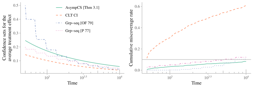
Figure 9: A comparison of 90% confidence sets for the average treatment effect in a simulated sequential experiment using (a) the AsympCS of Theorem 3.1, (b) the CLT-based CI, and the group-sequential repeated CIs of (c) O’Brien and Fleming [33], and (d) Pocock [36]. The group-sequential methods used a start time of $t_{1}=500$ and a maximal sample size of $t_{10}=10,000$ with $10$ logarithmically-spaced peeking times. The jagged drops in their widths correspond to CIs being updated at each peek. Notice in the left-hand side plot the group-sequential repeated CIs lie somewhere in between the AsympCS and the CLT CI (especially those using the Pocock boundary). Furthermore, notice in the right-hand side plot that the cumulative miscoverage rate of the AsympCS lies below $\alpha=0.1$ while the group-sequential CIs slightly exceed it. Nevertheless, those of the CLT-based CI’s miscoverage rates greatly exceed the other three, diverging quickly beyond $\alpha=0.1$ and exceeding $0.6$ by $t_{10}=10,000$.

Here, we provide a simulation comparing the widths and cumulative miscoverage rates of AsympCSs to two popular repeated CIs from the group-sequential literature — namely those of Pocock [36] and O’Brien and Fleming [33] and display the classical CLT-based CI alongside them for reference (Fig. 9). Perhaps unsurprisingly, group-sequential methods (and especially those using the boundary of Pocock [36]) tend to lie somewhere in between CLT CIs and AsympCSs. This added tightness over AsympCSs of course comes at the cost of less flexibility, especially in regards to continuous monitoring and unbounded time horizons discussed above.

B.5 The Lyapunov-type condition implies the Lindeberg-type condition

Here, we give a brief proof of the fact that the Lyapunov-type condition discussed in the paragraph following Theorem 2.5 indeed implies L-2.

Proof.

Suppose that the following Lyapunov-type condition holds with some $\delta>0$:

$$\sum_{t=1}^{\infty}\frac{\mathbb{E}\left(|X_{t}|^{2+\delta}\mid Y_{1}^{t-1}\right)}{\sqrt{V_{t}}^{2+\delta}}<\infty,$$ (184)

and we want to show that L-2 holds for some $\kappa\in(0,1)$. Indeed, set $\kappa:=\frac{1+\delta/2}{1+\delta}$. Note that $1\leq V_{t}^{-\kappa\delta/2}|X_{t}|^{\delta}$ whenever $X_{t}^{2}>V_{t}^{\kappa}$, and hence

$$\sum_{t=1}^{\infty}\frac{\mathbb{E}\left(X_{t}^{2}\mathds{1}\left\{X_{t}^{2}>V_{t}^{\kappa}\right\}\mid Y_{1}^{t-1}\right)}{V_{t}^{\kappa}} \leq\sum_{t=1}^{\infty}\frac{\mathbb{E}\left(V_{t}^{-\kappa\delta/2}|X_{t}|^{2+\delta}\mathds{1}\left\{X^{2}_{t}>V_{t}^{\kappa}\right\}\mid Y_{1}^{t-1}\right)}{V_{t}^{\kappa}}$$ (185)

$$=\sum_{t=1}^{\infty}\frac{\mathbb{E}\left(|X_{t}|^{2+\delta}\mathds{1}\left\{X^{2}_{t}>V_{t}^{\kappa}\right\}\mid Y_{1}^{t-1}\right)}{V_{t}^{\kappa(1+\delta/2)}}$$ (186)

$$=\sum_{t=1}^{\infty}\frac{\mathbb{E}\left(|X_{t}|^{2+\delta}\mid Y_{1}^{t-1}\right)}{\sqrt{V_{t}}^{2+\delta}}<\infty,$$ (187)

which completes the proof.

∎

B.6 The connections between “delayed start” boundaries and other works

As mentioned in Section 2.5, while we provided a definition for asymptotic time-uniform coverage in Definition 2.7, similar guarantees have appeared in past and followup works to ours. In the following two remarks, we elaborate on these connections and discuss how Proposition 2.9 can be viewed as a generalization and uniform improvement of these other works, and how Theorem 2.8 (the asymptotic coverage guarantee for our main AsympCSs) is new altogether.

Remark 5 (Relationship to Robbins and Siegmund).

Informally, Robbins and Siegmund [42, Theorem 2(i)] show that for independent and identically distributed random variables $(Y_{t})_{t=1}^{\infty}\sim\mathbb{P}$ with mean zero and unit variance, the probability of their partial sums $S_{t}:=\sum_{i=1}^{t}Y_{i}$ exceeding a boundary behaves like a rescaled Wiener process exceeding that boundary. For iid data with known variance, their result combined with Robbins’ delayed start [41, Eq. (20)] implies an asymptotic coverage guarantee (in the sense of Definition 2.7) for $\widetilde{C}_{t}^{\mathrm{DS}\star}$ given in (34) but with $\widehat{\sigma}_{t}$ replaced by the true $\sigma$. As such, (34) should be thought of as a generalization of Robbins and Robbins and Siegmund’s boundary when variances are unknown, and under martingale dependence. Nevertheless, Proposition 2.9 is strictly more general still, allowing for variances to never converge.

Remark 6 (Relationship to Bibaut et al. [2]).

In a recent preprint, and inspired by our current paper, Bibaut et al. [2] derive a particular boundary and show that it satisfies an asymptotic coverage guarantee in the sense of Definition 2.7, but Proposition 2.9 improves on this by (a) substantially weakening assumptions, (b) being uniformly tighter, and (c) removing unnecessary tuning parameters. Moreover, we accomplish (a)–(c) via rather different and arguably simpler techniques. Improvement (a) follows from the fact that their results implicitly make the same assumptions as (34) requiring that $\widetilde{\sigma}_{t}^{2}$ converges a.s. to a constant $\sigma_{\star}^{2}$. Improvement (b) follows easily by noting that after some algebraic manipulations, Bibaut et al.’s boundary is equivalent to $(\widetilde{C}_{t}^{\mathrm{DS}\star})_{t=1}^{\infty}$ given in (34) but with $1/t$ replaced by $(t+\lambda)/t^{2}$ and $\log(t/m)$ replaced by $\log((t+\lambda)/m)$ for some $\lambda>0$. Consequently, their boundary is always looser and would recover (34) if $\lambda$ were set to 0 but note that Bibaut et al. [2, Algorithm 1] requires strict positivity of $\lambda>0$ as it has $1/\lambda$ terms in it, (but their proofs can be amended via our techniques to eliminate $1/\lambda$ altogether). Nevertheless, both Bibaut et al. [2] and (34) require $\widetilde{\sigma}_{t}^{2}$ to converge a.s. while Proposition 2.9 does not, so we always recommend using $(\widetilde{C}_{t}^{\mathrm{DS}})_{t=1}^{\infty}$ for all practical purposes. We end by noting that it was their paper that inspired us to explicitly define Definition 2.7 and show that it can hold for more general boundaries (e.g. in Theorem 2.8) and under weaker conditions (such as in Theorem 2.8 and Proposition 2.9). Indeed, one could derive a general framework for asymptotic coverage akin to Lemma 2.4 but we omit this for brevity.

B.7 A brief review of efficient estimators

For a detailed account of efficient estimation in semiparametric models, we refer readers to Bickel et al. [3], van der Vaart [59], van der Laan and Robins [55], Tsiatis [53] and Kennedy [24], but we provide a brief overview of their fundamental relevance to estimation of the ATE here.

A central goal of semiparametric efficiency theory is to characterize the set of influence functions of $\psi$ — the summands found in sample averages forming consistent and asymptotically normal regular estimators of $\psi$. Of particular interest is finding the efficient influence function (EIF) as it is the one with the smallest variance (which itself acts as a semiparametric analogue of the Cramer-Rao lower bound), hence providing a benchmark for constructing optimal estimators, at least in an asymptotic local minimax sense. In the case of $\psi$, the (uncentered) EIF is given by

$$f(z)\equiv f(x,a,y):=\left\{\mu^{1}(x)-\mu^{0}(x)\right\}+\left(\frac{a}{\pi(x)}-\frac{1-a}{1-\pi(x)}\right)\left\{y-\mu^{a}(x)\right\},$$ (188)

where $\mu^{a}(x):=\mathbb{E}\left(Y\mid X=x,A=a\right)$ is the regression function among those treated at level $a\in\{0,1\}$ and $\pi(x):=\mathbb{P}\left(A=1\mid X=x\right)$ is the propensity score (i.e. probability of treatment) for an individual with covariates $x$. In particular, this means that no estimator of $\psi$ based on $t$ observations can have asymptotic mean squared error smaller than $\operatorname{\mathrm{var}}(f(Z))/t$ without imposing additional assumptions.

Of course, the exact values of $\eta:=(\mu^{1},\mu^{0},\pi)$ are not known in general — $\pi$ is only known in randomized experiments, but not observational studies, while $(\mu^{1},\mu^{0})$ are typically not known in either. As such, we will need to replace these “nuisance functions” $\eta$ with data-dependent estimates $\widehat{\eta}$, but using the same data to construct estimators $\widehat{\eta}$ and $\widehat{f}$ for both $\eta$ and $f$ (sometimes referred to as “double-dipping”) complicates the analysis of the downstream estimator of $\psi$. A clever and simple remedy used throughout the semiparametric literature is to split the sample, whereby a random subset of the data are used to estimate $\eta$, while the remaining data are used to construct $\widehat{f}$, greatly simplifying the downstream analysis [43, 67, 8].

In a randomized experiment, the joint distribution of $(X,Y)$ is unknown but the conditional distribution of $A\mid X=x$ is known to be Bernoulli($\pi(x)$) by design. In this case, our statistical model for $Z$ is a proper semiparametric model, and hence there are infinitely many influence functions, all of which take the form,

$$\widebar{f}(z)\equiv\widebar{f}(x,a,y):=\left\{\widebar{\mu}^{1}(x)-\widebar{\mu}^{0}(x)\right\}+\left(\frac{a}{\pi(x)}-\frac{1-a}{1-\pi(x)}\right)\left\{y-\widebar{\mu}^{a}(x)\right\},$$ (189)

where $\widebar{\mu}^{a}:\mathbb{R}^{d}\mapsto\mathbb{R}$ is any function. However, when the joint distribution of $(X,A,Y)$ is left completely unspecified (such as in an observational study with unknown propensity scores), our statistical model for $\mathbb{P}$ is nonparametric, and hence there is only one influence function, the EIF given in (188).

Not only does the EIF $f(z)$ provide us with a benchmark against which to compare estimators, but it hints at the first step in deriving the most efficient estimator. Namely, $\frac{1}{t}\sum_{i=1}^{t}f(Z_{i})$ is a consistent estimator for $\psi$ with asymptotic variance equal to the efficiency bound, $\operatorname{\mathrm{var}}(f)$ by construction. However, $f(Z)$ depends on possibly unknown nuisance functions $\eta:=(\mu^{1},\mu^{0},\pi)$. A natural next step would be to simply estimate $\eta$ from the data $(Z_{t})_{{t}={1}}^{\infty}$. Crucially, it is possible to ensure that only a negligible amount of additional estimation error is incurred by replacing $\eta$ by a data-dependent estimate $\widehat{\eta}_{t}$ — the essential technique here being sample splitting and cross-fitting [43, 67, 8]. In the following section, we introduce sequential sample-splitting and cross-fitting, allowing the same types of analyses of $\widehat{\eta}_{t}$ to be carried out but in fully sequential settings.

B.8 Unimprovability of AsympCSs using efficient influence functions

Consider the confidence sequence of Theorem 3.2,

$$\widehat{\psi}_{t}^{\times}\pm\underbrace{\sqrt{\widehat{\operatorname{\mathrm{var}}}_{t}(\widehat{f})}}_{(iii)}\cdot\underbrace{\sqrt{\frac{2(t\rho^{2}+1)}{t^{2}\rho^{2}}\log\left(\frac{\sqrt{t\rho^{2}+1}}{\alpha}\right)}}_{(i)}~{}~{}~{}\text{with rate}~{}\underbrace{o\left(\sqrt{\frac{\log\log t}{t}}\right)}_{(ii)}.$$ (190)

It is natural to whether (190) can be tightened at all. In a certain sense, (190) inherits optimality from its three main components: $(i)$ Robbins’ normal mixture boundary, $(ii)$ the approximation error rate, and $(iii)$ the estimated standard deviation $\sqrt{\widehat{\operatorname{\mathrm{var}}}_{t}(\widehat{f})}$ of the efficient influence function $f$.

Term (i)

Starting with the width, we have that in the case of iid Gaussian data $G_{1},G_{2},\dots\sim\mathcal{N}(\mu,\sigma^{2})$, Robbins’ normal mixture confidence sequence [41] is obtained by first showing that

$$M_{t}(\mu):=\exp\left\{\frac{\rho^{2}(\sum_{i=1}^{t}(G_{i}-\mu))^{2}}{2(t\rho^{2}+1)}\right\}(t\rho^{2}+1)^{-1/2}$$

is a nonnegative martingale starting at one, and hence by Ville’s inequality [62],

$$\mathbb{P}(\exists t\geq 1:M_{t}(\mu)\geq 1/\alpha)\leq\alpha.$$

The resulting confidence sequence $\widebar{C}_{t}^{\mathcal{N}}$ at each time $t$ is defined as the set of $m$ such that $M_{t}(m)<1/\alpha$, i.e. $\widebar{C}_{t}^{\mathcal{N}}:=\{m\in\mathbb{R}:M_{t}(m)<1/\alpha\}$ and consequently,

$$\mathbb{P}(\exists t\geq 1:\mu\notin\widebar{C}_{t}^{\mathcal{N}})=\mathbb{P}(\exists t\geq 1:M_{t}(\mu)\geq 1/\alpha)\leq\alpha.$$

This inequality is extremely tight, since Ville’s inequality almost holds with equality for nonnegative martingales. Technically, the paths of the martingale need to be continuous for equality to hold, which can only happen in continuous time (such as for a Wiener process). However, any deviation from equality only holds because of this “overshoot” and in practice, the error probability is almost exactly $\alpha$. This means that the normal mixture confidence sequence $\widebar{C}_{t}^{\mathcal{N}}$ cannot be uniformly tightened: any improvement for some times will necessarily result in looser bounds for others. For a precise characterization of this optimality for the (sub)-Gaussian case, see Howard et al. [19, Section 3.6], or Ramdas et al. [40] for a more general discussion of admissible confidence sequences.

Term (ii)

The error incurred from almost-surely approximating a sample average $\frac{1}{t}\sum_{i=1}^{t}f(Z_{i})$ of influence functions by Gaussian random variables is a direct consequence of Strassen [50] and improvements under $q>2$ finite absolute moments by Komlós, Major, and Tusnády [26, 27] and Major [31], which are unimprovable without additional assumptions. Further approximation errors result from using $\widehat{\operatorname{\mathrm{var}}}_{t}(\widehat{f})$ to estimate $\operatorname{\mathrm{var}}(f)$, where almost-sure law of the iterated logarithm rates appear, and are themselves unimprovable.

Term (iii)

Using the approximations mentioned in $(ii)$ permits the use of Robbins’ normal mixture confidence sequence in $(i)$. However, a factor of $\sqrt{\widehat{\operatorname{\mathrm{var}}}_{t}(\widehat{f})}$ necessarily appears in front of the width as an estimate of the standard deviation $\sqrt{\operatorname{\mathrm{var}}(f)}$ of the efficient influence function $f$ discussed in Section 3. Importantly, $\sqrt{\operatorname{\mathrm{var}}(f)}$ corresponds to the semiparametric efficiency bound, so that no estimator of $\psi$ can have asymptotic mean squared error smaller than $\operatorname{\mathrm{var}}(f(Z))/t$ without imposing additional assumptions [59].

References

- Bahadur and Savage [1956] Raghu R Bahadur and Leonard J Savage. The nonexistence of certain statistical procedures in nonparametric problems. The Annals of Mathematical Statistics, 27(4):1115–1122, 1956.
- Bibaut et al. [2022] Aurélien Bibaut, Nathan Kallus, and Michael Lindon. Near-optimal non-parametric sequential tests and confidence sequences with possibly dependent observations. arXiv preprint arXiv:2212.14411, 2022.
- Bickel et al. [1993] Peter J Bickel, Chris AJ Klaassen, Ya’acov Ritov, and Jon A Wellner. Efficient and adaptive estimation for semiparametric models, volume 4. Johns Hopkins University Press Baltimore, 1993.
- Billingsley [1995] Patrick Billingsley. Probability and measure (3rd ed.). John Wiley & Sons, 1995.
- Breiman [1996] Leo Breiman. Stacked regressions. Machine learning, 24(1):49–64, 1996.
- Breiman [2001] Leo Breiman. Random forests. Machine learning, 45(1):5–32, 2001.
- Chatterjee [2012] Sourav Chatterjee. A new approach to strong embeddings. Probability Theory and Related Fields, 152(1-2):231–264, 2012.
- Chernozhukov et al. [2018] Victor Chernozhukov, Denis Chetverikov, Mert Demirer, Esther Duflo, Christian Hansen, Whitney Newey, and James Robins. Double/debiased machine learning for treatment and structural parameters. The Econometrics Journal, 21(1):C1–C68, 2018.
- Corless et al. [1996] Robert M Corless, Gaston H Gonnet, David EG Hare, David J Jeffrey, and Donald E Knuth. On the Lambert W function. Advances in Computational mathematics, 5(1):329–359, 1996.
- Darling and Robbins [1967] D. A. Darling and Herbert E. Robbins. Confidence sequences for mean, variance, and median. Proceedings of the National Academy of Sciences of the United States of America, 58 1:66–8, 1967.
- Díaz and van der Laan [2012] Iván Díaz and Mark van der Laan. Population intervention causal effects based on stochastic interventions. Biometrics, 68(2):541–549, 2012.
- Efron [1971] Bradley Efron. Forcing a sequential experiment to be balanced. Biometrika, 58(3):403–417, 1971.
- Einmahl [1989] Uwe Einmahl. Extensions of results of Komlós, Major, and Tusnády to the multivariate case. Journal of multivariate analysis, 28(1):20–68, 1989.
- Einmahl [2009] Uwe Einmahl. A new strong invariance principle for sums of independent random vectors. Journal of Mathematical Sciences, 163(4):311–327, 2009.
- Hastie and Tibshirani [1990] Trevor J Hastie and Robert J Tibshirani. Generalized additive models, volume 43. CRC press, 1990.
- Hoeffding [1963] Wassily Hoeffding. Probability Inequalities for Sums of Bounded Random Variables. Journal of the American Statistical Association, 58(301):13–30, 1963.
- Howard and Ramdas [2022] Steven R Howard and Aaditya Ramdas. Sequential estimation of quantiles with applications to A/B-testing and best-arm identification. Bernoulli, 2022.
- Howard et al. [2020] Steven R. Howard, Aaditya Ramdas, Jon McAuliffe, and Jasjeet Sekhon. Time-uniform Chernoff bounds via nonnegative supermartingales. Probability Surveys, 17:257–317, 2020.
- Howard et al. [2021] Steven R Howard, Aaditya Ramdas, Jon McAuliffe, and Jasjeet Sekhon. Time-uniform, nonparametric, nonasymptotic confidence sequences. The Annals of Statistics, 2021.
- Jennison and Turnbull [1999] Christopher Jennison and Bruce W Turnbull. Group sequential methods with applications to clinical trials. CRC Press, 1999.
- Johari et al. [2017] Ramesh Johari, Pete Koomen, Leonid Pekelis, and David Walsh. Peeking at A/B tests: Why it matters, and what to do about it. In Proceedings of the 23rd ACM SIGKDD International Conference on Knowledge Discovery and Data Mining, pages 1517–1525, 2017.
- Johnson and Pollard [2018] Alistair Johnson and Tom Pollard. sepsis3-mimic, May 2018. URL https://doi.org/10.5281/zenodo.1256723.
- Johnson et al. [2016] Alistair EW Johnson, Tom J Pollard, Lu Shen, Li-wei H Lehman, Mengling Feng, Mohammad Ghassemi, Benjamin Moody, Peter Szolovits, Leo Anthony Celi, and Roger G Mark. MIMIC-III, a freely accessible critical care database. Scientific data, 3:160035, 2016.
- Kennedy [2016] Edward H Kennedy. Semiparametric theory and empirical processes in causal inference. In Statistical causal inferences and their applications in public health research, pages 141–167. Springer, 2016.
- Kennedy et al. [2020] Edward H Kennedy, Sivaraman Balakrishnan, and Max G’Sell. Sharp instruments for classifying compliers and generalizing causal effects. Annals of Statistics, 48(4):2008–2030, 2020.
- Komlós et al. [1975] János Komlós, Péter Major, and Gábor Tusnády. An approximation of partial sums of independent rv’-s, and the sample df. i. Zeitschrift für Wahrscheinlichkeitstheorie und verwandte Gebiete, 32(1-2):111–131, 1975.
- Komlós et al. [1976] János Komlós, Péter Major, and Gábor Tusnády. An approximation of partial sums of independent rv’s, and the sample df. ii. Zeitschrift für Wahrscheinlichkeitstheorie und verwandte Gebiete, 34(1):33–58, 1976.
- Lai [1976a] Tze Leung Lai. Boundary crossing probabilities for sample sums and confidence sequences. The Annals of Probability, pages 299–312, 1976a.
- Lai [1976b] Tze Leung Lai. On confidence sequences. The Annals of Statistics, 4(2):265–280, 1976b.
- Lindeberg [1922] Jarl Waldemar Lindeberg. Eine neue herleitung des exponentialgesetzes in der wahrscheinlichkeitsrechnung. Mathematische Zeitschrift, 15(1):211–225, 1922.
- Major [1976] Péter Major. The approximation of partial sums of independent rv’s. Zeitschrift für Wahrscheinlichkeitstheorie und verwandte Gebiete, 35(3):213–220, 1976.
- Morrow and Philipp [1982] Gregory Morrow and Walter Philipp. An almost sure invariance principle for hilbert space valued martingales. Transactions of the American Mathematical Society, pages 231–251, 1982.
- O’Brien and Fleming [1979] Peter C O’Brien and Thomas R Fleming. A multiple testing procedure for clinical trials. Biometrics, pages 549–556, 1979.
- Pace and Salvan [2020] Luigi Pace and Alessandra Salvan. Likelihood, replicability and robbins’ confidence sequences. International Statistical Review, 88(3):599–615, 2020.
- Petrov [2022] Valentin V Petrov. Sums of independent random variables. In Sums of Independent Random Variables. De Gruyter, 2022.
- Pocock [1977] Stuart J Pocock. Group sequential methods in the design and analysis of clinical trials. Biometrika, 64(2):191–199, 1977.
- Pollard and Johnson [2016] Tom J Pollard and Alistair EW Johnson. The MIMIC-III Clinical Database. http://dx.doi.org/10.13026/C2XW26, 2016.
- Polley and van der Laan [2010] Eric C Polley and Mark J van der Laan. Super learner in prediction. U.C. Berkeley Division of Biostatistics Working Paper Series, (Working paper 222), 2010.
- Polley et al. [2011] Eric C Polley, Sherri Rose, and Mark J van der Laan. Super learning. In Targeted learning, pages 43–66. Springer, 2011.
- Ramdas et al. [2020] Aaditya Ramdas, Johannes Ruf, Martin Larsson, and Wouter Koolen. Admissible anytime-valid sequential inference must rely on nonnegative martingales. arXiv preprint arXiv:2009.03167, 2020.
- Robbins [1970] Herbert Robbins. Statistical methods related to the law of the iterated logarithm. The Annals of Mathematical Statistics, 41(5):1397–1409, 1970.
- Robbins and Siegmund [1970] Herbert Robbins and David Siegmund. Boundary crossing probabilities for the Wiener process and sample sums. The Annals of Mathematical Statistics, pages 1410–1429, 1970.
- Robins et al. [2008] James Robins, Lingling Li, Eric Tchetgen Tchetgen, Aad van der Vaart, et al. Higher order influence functions and minimax estimation of nonlinear functionals. In Probability and statistics: essays in honor of David A. Freedman, pages 335–421. Institute of Mathematical Statistics, 2008.
- Robins et al. [1994] James M Robins, Andrea Rotnitzky, and Lue Ping Zhao. Estimation of regression coefficients when some regressors are not always observed. Journal of the American Statistical Association, 89(427):846–866, 1994.
- Rotnitzky et al. [1998] Andrea Rotnitzky, James M Robins, and Daniel O Scharfstein. Semiparametric regression for repeated outcomes with nonignorable nonresponse. Journal of the American Statistical Association, 93(444):1321–1339, 1998.
- Scharfstein et al. [1999] Daniel O Scharfstein, Andrea Rotnitzky, and James M Robins. Adjusting for nonignorable drop-out using semiparametric nonresponse models. Journal of the American Statistical Association, 94(448):1096–1120, 1999.
- Shahn et al. [2020] Zach Shahn, Nathan I Shapiro, Patrick D Tyler, Daniel Talmor, and H Lehman Li-wei. Fluid-limiting treatment strategies among sepsis patients in the icu: a retrospective causal analysis. Critical Care, 24(1):1–9, 2020.
- Singer et al. [2016] Mervyn Singer, Clifford S Deutschman, Christopher Warren Seymour, Manu Shankar-Hari, Djillali Annane, Michael Bauer, Rinaldo Bellomo, Gordon R Bernard, Jean-Daniel Chiche, Craig M Coopersmith, et al. The third international consensus definitions for sepsis and septic shock (sepsis-3). Jama, 315(8):801–810, 2016.
- Skorokhod [1961] AV Skorokhod. Research on the theory of random processes. Kiev Univ, 1961.
- Strassen [1964] Volker Strassen. An invariance principle for the law of the iterated logarithm. Zeitschrift für Wahrscheinlichkeitstheorie und verwandte Gebiete, 3(3):211–226, 1964.
- Strassen [1967] Volker Strassen. Almost sure behavior of sums of independent random variables and martingales. In Proceedings of the Fifth Berkeley Symposium on Mathematical Statistics and Probability, volume 3, page 315. University of California Press, 1967.
- Tao [2012] Terence Tao. E pluribus unum: from complexity, universality. Daedalus, 141(3):23–34, 2012.
- Tsiatis [2007] Anastasios Tsiatis. Semiparametric theory and missing data. Springer Science & Business Media, 2007.
- Tsybakov [2003] Alexandre B Tsybakov. Optimal rates of aggregation. In Learning theory and kernel machines, pages 303–313. Springer, 2003.
- van der Laan and Robins [2003] Mark J van der Laan and James M Robins. Unified methods for censored longitudinal data and causality. Springer Science & Business Media, 2003.
- van der Laan and Rose [2011] Mark J van der Laan and Sherri Rose. Targeted learning: causal inference for observational and experimental data. Springer Science & Business Media, 2011.
- van der Laan et al. [2007] Mark J van der Laan, Eric C Polley, and Alan E Hubbard. Super learner. Statistical applications in genetics and molecular biology, 6(1), 2007.
- van der Vaart [2000] Aad W van der Vaart. Asymptotic statistics, volume 3. Cambridge university press, 2000.
- van der Vaart [2002] Aad W van der Vaart. Semiparametric statistics. Lecture Notes in Math., 2002.
- van der Vaart et al. [2006] Aad W van der Vaart, Sandrine Dudoit, and Mark J van der Laan. Oracle inequalities for multi-fold cross validation. Statistics and Decisions, 24(3):351–371, 2006.
- van Walraven et al. [2009] Carl van Walraven, Peter C Austin, Alison Jennings, Hude Quan, and Alan J Forster. A modification of the elixhauser comorbidity measures into a point system for hospital death using administrative data. Medical care, pages 626–633, 2009.
- Ville [1939] Jean Ville. Etude critique de la notion de collectif. Bull. Amer. Math. Soc, 45(11):824, 1939.
- Wang and Ramdas [2022] Hongjian Wang and Aaditya Ramdas. Catoni-style confidence sequences for heavy-tailed mean estimation. arXiv preprint arXiv:2202.01250, 2022.
- Wasserman et al. [2020] Larry Wasserman, Aaditya Ramdas, and Sivaraman Balakrishnan. Universal inference. Proceedings of the National Academy of Sciences, 117(29):16880–16890, 2020.
- Waudby-Smith and Ramdas [2023] Ian Waudby-Smith and Aaditya Ramdas. Estimating means of bounded random variables by betting. Journal of the Royal Statistical Society, Series B (with discussion), 2023.
- Yu et al. [2020] Miao Yu, Wenbin Lu, and Rui Song. A new framework for online testing of heterogeneous treatment effect. In Proceedings of the AAAI Conference on Artificial Intelligence, volume 34, pages 10310–10317, 2020.
- Zheng and van der Laan [2010] Wenjing Zheng and Mark J van der Laan. Asymptotic theory for cross-validated targeted maximum likelihood estimation. U.C. Berkeley Division of Biostatistics Working Paper Series, (Working paper 273), 2010.