Generalizable Episodic Memory for Deep Reinforcement Learning

Supplementary Material

Abstract

Episodic memory-based methods can rapidly latch onto past successful strategies by a non-parametric memory and improve sample efficiency of traditional reinforcement learning. However, little effort is put into the continuous domain, where a state is never visited twice, and previous episodic methods fail to efficiently aggregate experience across trajectories. To address this problem, we propose Generalizable Episodic Memory (GEM), which effectively organizes the state-action values of episodic memory in a generalizable manner and supports implicit planning on memorized trajectories. GEM utilizes a double estimator to reduce the overestimation bias induced by value propagation in the planning process. Empirical evaluation shows that our method significantly outperforms existing trajectory-based methods on various MuJoCo continuous control tasks. To further show the general applicability, we evaluate our method on Atari games with discrete action space, which also shows a significant improvement over baseline algorithms.

1 Introduction

Deep reinforcement learning (RL) has been tremendously successful in various domains, like classic games (Silver et al., 2016), video games (Mnih et al., 2015), and robotics (Lillicrap et al., 2016). However, it still suffers from high sample complexity, especially compared to human learning (Tsividis et al., 2017). One significant deficit comes from gradient-based bootstrapping, which is incremental and usually very slow (Botvinick et al., 2019).

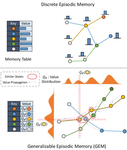
Figure 1: Illustration of our basic idea. Conventional episodic memory usually uses a non-parametric schema to store every state-action pairs and updates their values when re-encountering the same events. Instead, generalizable episodic memory stores the $Q$-values for each event by a parametric network $\mathcal{M}_{\theta}$ so that each single event can generalize to their neighborhoods. We further perform value propagation along adjacent states to encourage information exchange between related events.

Inspired by psychobiological studies of human’s episodic memory (Sutherland & Rudy, 1989; Marr et al., 1991; Lengyel & Dayan, 2007) and instance-based decision theory (Gilboa & Schmeidler, 1995), episodic reinforcement learning (Blundell et al., 2016; Pritzel et al., 2017; Lin et al., 2018; Hansen et al., 2018; Zhu et al., 2020) presents a non-parametric or semi-parametric framework that fast retrieves past successful strategies to improve sample efficiency. Episodic memory stores past best returns, and the agents can act accordingly to repeat the best outcomes without gradient-based learning.

However, most existing methods update episodic memory only by exactly re-encountered events, leaving the generalization ability aside. As Heraclitus, the Greek philosopher, once said, “No man ever steps in the same river twice.” (Kahn et al., 1981) Similarly, for an RL agent acting in continuous action and state spaces, the same state-action pair can hardly be observed twice. However, humans can connect and retrospect from similar experiences of different times, with no need to re-encounter the same event (Shohamy & Wagner, 2008). Inspired by this human’s ability to learn from generalization, we propose Generalizable Episodic Memory (GEM), a novel framework that integrates the generalization ability of neural networks and the fast retrieval manner of episodic memory.

We use Figure 1 to illustrate our basic idea. Traditional discrete episodic control methods usually build a non-parametric slot-based memory table to store state-value pairs of historical experiences. In the discrete domain, states can be re-encountered many times. This re-encountering enables traditional methods to aggregate trajectories by directly taking maximum among all historical returns. However, this is not feasible in environments with high dimensional states and action space, especially in the continuous domain, where an agent will never visit the same state twice. On the contrary, GEM learns a virtual memory table memorized by deep neural networks to aggregate similar state-action pairs that essentially have the same nature. This virtual table naturally makes continuous state-action pairs generalizable by reconstructing experiences’ latent topological structure with neural networks. This memory organization enables planning across different trajectories, and GEM uses this capability to do implicit planning by performing value propagation along trajectories saved in the memory and calculating the best sequence over all possible real and counterfactual combinatorial trajectories.

We further propose to use twin networks to reduce the overestimation of these aggregated returns. Merely taking maximum among all possible plans leads to severe overestimation since overestimated values are preserved along the trajectory. Thus, we use two networks to separately calculate which trajectory has the maximal value and how large the maximum value is, which shares the similar idea with double Q-learning (van Hasselt, 2010).

The main contribution of our proposed method is threefold: 1. We present a novel framework inspired by psychology, GEM, to build generalizable episodic memory and improve sample efficiency. GEM consists of a novel value planning scheme for the continuous domain and a twin back-propagation process to reduce overestimation along the trajectories; 2. We formally analyze the estimation and convergence properties of our proposed algorithm; 3. We empirically show the significant improvement of GEM over other baseline algorithms and its general applicability across continuous and discrete domains. Besides, we analyze the effectiveness of each part of GEM by additional comparisons and ablation studies.

2 Preliminaries

We consider a Markov Decision Process (MDP), defined by the tuple $\langle\mathcal{S},\mathcal{A},P,r,\gamma\rangle$, where $\mathcal{S}$ is the state space and $\mathcal{A}$ the action space. $P(\cdot|s,a):\mathcal{S}\times\mathcal{A}\times\mathcal{S}\rightarrow\mathbb{R}$ denotes the transition distribution function and $r(s,a):\mathcal{S}\times\mathcal{A}\rightarrow\mathbb{R}$ the reward function. $\gamma\in[0,1)$ is the discount factor.

The goal of an RL agent is to learn a policy $\pi:\mathcal{S}\times\mathcal{A}\rightarrow\mathbb{R}$ which maximizes the expectation of a discounted cumulative reward, i.e.,

$$J(\pi)=\operatorname{\mathbb{E}}_{\begin{subarray}{c}s_{0}\sim\rho_{0},a_{t}\sim\pi(\cdot|s_{t}),\\ s_{t+1}\sim P(\cdot|s_{t},a_{t})\end{subarray}}\left[\sum_{t=0}^{\infty}\gamma^{t}r(s_{t},a_{t})\right],$$

where $\rho_{0}$ denotes the distribution of initial states.

2.1 Deterministic Policy Gradient

In the context of continuous control, actor-critic architecture is widely used (Sutton et al., 1999; Peters & Bagnell, 2010) to handle the continuous action space. In actor-critic framework, a critic $Q_{\theta}$ is used to estimate the action-value function $Q_{\theta}(s,a)\approx Q^{\pi}(s,a)$, while the parametric actor $\pi_{\phi}$ optimizes its policy using the policy gradient from parametric $Q_{\theta}$. When $\pi_{\phi}$ is a deterministic function, the gradient can be expressed as follows:

$$\nabla_{\phi}J(\pi_{\phi})=\operatorname{\mathbb{E}}_{s\sim p_{\pi}}[\nabla_{a}Q_{\theta}(s,a)|_{a=\pi(s)}\nabla_{\phi}\pi_{\phi}(s)],$$

which is known as deterministic policy gradient theorem (Silver et al., 2014).
$Q_{\theta}$ can be learned from the TD-target derived from the Bellman Equation (Bellman, 1957):

$$y=r(s,a)+\gamma Q_{\theta^{\prime}}(s^{\prime},a^{\prime}),a^{\prime}\sim\pi_{\phi}(s^{\prime})$$

In the following section, when it does not lead to confusion, we use $Q_{\theta}(s)$ instead of $Q_{\theta}(s,\pi_{\phi}(s))$ for simplicity.

2.2 Double Q-Learning

Q-learning update state-action values by the TD target (Sutton, 1988a) :

$$r+\gamma\max_{a}Q(s^{\prime},a).$$

However, the max operator in the target can easily lead to overestimation, as discussed in van Hasselt (2010). Thus, They propose to estimate the maximum $Q$-values over all actions $\max_{a}Q(s,a)$ using the double estimator, i.e.,

$$Q_{\text{double}}(s)=Q^{A}(s,a^{*}_{B}),a^{*}_{B}=\operatorname*{arg\,max}_{a}Q^{B}(s,a),$$

where $Q^{A},Q^{B}$ are two independent function approximators for $Q$-values.

2.3 Model-Free Episodic Control

Traditional deep RL approaches suffer from sample inefficiency because of slow gradient-based updates. Episodic control is proposed to speed up the learning process by a non-parametric episodic memory (EM). The key idea is to store good past experiences in a tabular-based non-parametric memory and rapidly latch onto past successful policies when encountering similar states, instead of waiting for many steps of optimization. When different experiences meet up at the same state-action pair $(s,a)$, model-free episodic control (MFEC; Blundell et al., 2016) aggregates the values of different trajectories by taking the maximum return $R$ among all these rollouts starting from the intersection $(s,a)$. Specifically, $Q^{EM}$ is updated by the following equation:

$$Q^{EM}(s,a)=\left\{\begin{aligned} &R,&\text{if~{}}(s,a)\notin EM,\\ &\max{\{R,Q^{EM}(s,a)\}},&\text{otherwise.}\\ \end{aligned}\right.$$ (1)

At the execution time, MFEC selects the action according to the maximum $Q$-value of the current state. If there is no exact match of the state, MFEC performs a $k$-nearest-neighbors lookup to estimate the state-action values, i.e.,

$$\widehat{Q}^{EM}(s,a)=\left\{\begin{aligned} &\frac{1}{k}\sum_{i=1}^{k}Q(s_{i},a),&\mbox{if }(s,a)\notin Q^{EM},\\ &Q^{EM}(s,a),&\mbox{otherwise},\\ \end{aligned}\right.$$ (2)

where $s_{i}$ $(i=1,\cdots,k)$ are the $k$ nearest states from $s$.

3 Generalizable Episodic Memory

3.1 Overview

In generalizable episodic memory (GEM), we use a parametric network $\mathcal{M}_{\theta}$ to represent the virtual memory table with parameter $\theta$, which is learned from tabular memory $\mathcal{M}$. To leverage the generalization ability of $\mathcal{M}_{\theta}$, we enhance the returns stored in the tabular memory by propagating value estimates from ${\mathcal{M}}_{\theta}$ and real returns from $\mathcal{M}$ along trajectories in the memory and take the best value over all possible rollouts, as depicted in Equation (4). Generalizable memory $\mathcal{M}_{\theta}$ is trained by performing regression toward this enhanced target and is then used to guide policy learning as well as to build the new target for GEM’s learning.

A significant issue for the procedure above is the overestimation induced from taking the best value along the trajectory. Overestimated values are preserved when doing back-propagation along the trajectory and hinder learning efficiency. To mitigate this issue, we propose to use twin networks for the back-propagation of value estimates. This twin back-propagation process uses the double estimator for estimating the maximum along trajectories, which resembles the idea of Double Q-learning (van Hasselt, 2010) and is illustrated in detail in Section 3.4. It is well known that vanilla reinforcement learning algorithms with function approximation already has a tendency to overestimate (van Hasselt, 2010; Fujimoto et al., 2018), making the overestimation reduction even more critical. To solve this challenge, we propose to use additional techniques to make the value estimation from $\mathcal{M}_{\theta}$ more conservative, which is illustrated in Section 3.5.

A formal description for GEM algorithm is shown in Algorithm 1. In the following sections, we use $Q_{\theta}$ to represent $Q_{\mathcal{M}_{\theta}}$ for simplicity. Our implementation of GEM is available at https://github.com/MouseHu/GEM.

Algorithm 1 Generalizable Episodic Memory

  Initialize episodic memory(critic) networks $Q^{(1)}_{\theta},Q^{(2)}_{\theta}$, and actor network $\pi_{\phi}$ with parameters $\theta_{(1)},\theta_{(2)},\phi$

  Initialize targets $\theta_{(1)}^{\prime}\leftarrow\theta_{(1)},\theta_{(2)}^{\prime}\leftarrow\theta_{(2)},\phi^{\prime}\leftarrow\phi$

  Initialize episodic memory $\mathcal{M}$

  for $t=1,\dots,T$ do

     Select action with noise $a\sim\pi(s)+\mathcal{N}(0,\sigma)$ 

     Observe reward $r$ and new state $s^{\prime}$ 

     Store transition tuple $(s,a,r,s^{\prime})$ in $\mathcal{M}$ 

     for  $i\in\{1,2\}$  do

        Sample $N$ transitions $(s_{t},a_{t},r_{t},s^{\prime}_{t},R_{t}^{(i)})$ from $\mathcal{M}$ 

        Update $\theta_{(i)}\leftarrow\min_{\theta_{(i)}}\sum(R_{t}^{(i)}-Q_{\theta}^{(i)}(s_{t},a_{t}))^{2}$ 

     end for

     if $t\mbox{ mod }u=0$ then

        $\phi^{\prime}\leftarrow\tau\phi+(1-\tau)\phi^{\prime}$ 

        $\theta_{(i)}^{\prime}\leftarrow\tau\theta_{(i)}+(1-\tau)\theta_{(i)}^{\prime}$ 

        Update Memory() 

     end if

     if $t\mbox{ mod }p=0$ then

        Update $\phi$ by the deterministic policy gradient 

        $\nabla_{\phi}J(\phi)=\nabla_{a}Q_{\theta_{1}}(s,a)|_{a=\pi_{\phi}(s)}\nabla_{\phi}\pi_{\phi(s)}$ 

     end if

  end for

Algorithm 2 Update Memory

  for trajectory $\tau$ in tabular memory $\mathcal{M}$ do

     for $s_{t},a_{t},r_{t},s_{t+1}$ in reversed($\tau$) do

        $\tilde{a}_{t+1}\sim\pi_{\phi^{\prime}}(s_{t+1})+\text{clip}(\mathcal{N}(0,\tilde{\sigma}),-c,c)$ 

        Compute $Q_{\theta^{\prime}_{(1,2)}}(s_{t+1},\tilde{a}_{t+1})$

        Compute $V_{t,h}^{(1,2)}$ with Equation (7) for $h$ in $0:T-t$

        Compute $R_{t}^{(1,2)}$ with Equation (8) and save into buffer $\mathcal{M}$

     end for

  end for

3.2 Generalizable Episodic Memory

Traditional discrete episodic memory is stored in a lookup table, learned as in Equation (2) and used as in Equation (1). This kind of methods does not consider generalization when learning values and enjoy little generalization ability from non-parametric nearest-neighbor search with random projections during execution. To enable the generalizability of such episodic memory, we use the parametric network $\mathcal{M}_{\theta}$ to learn and store values. As stated in Section 3.1, this parametric memory is learned by doing regression toward the best returns $R_{t}$ starting from the state-action pair $(s_{t},a_{t})$:

$$\mathcal{L}(Q_{\theta})=\operatorname{\mathbb{E}}_{(s_{t},a_{t},R_{t})\sim\mathcal{M}}(Q_{\theta}(s_{t},a_{t})-R_{t})^{2}.$$ (3)

where $R_{t}$ is computed from implicit planning over both real returns in tabular memory $\mathcal{M}$ and estimates in target generalizable memory table $\mathcal{M}_{\theta}^{\prime}$, as depicted in the next section. This learned virtual memory table is then used for both policy learning and building new target.

3.3 Implicit Memory-Based Planning

To leverage the analogical reasoning ability of our parametric memory, GEM conducts implicit memory-based planning to estimate the value for the best possible rollout for each state-action pair. At each step, GEM compares the best return so far along the trajectory with the value estimates from $Q_{\theta}$ and takes the maximum between them. $Q_{\theta}$ is generalized from similar experiences and can be regraded as the value estimates for counterfactual trajectories. This procedure is conducted recursively from the last step to the first step along the trajectory, forming an implicit planning scheme within episodic memory to aggregate experiences along and across trajectories. The overall back-propagation process can be written in the following form:

$$R_{t}=\left\{\begin{aligned} &r_{t}+\gamma\max(R_{t+1},Q_{\theta}(s_{t+1},a_{t+1}))&\mbox{if }t<T,\\ &r_{t}&\mbox{if }t=T,\\ \end{aligned}\right.$$ (4)

where $t$ denotes steps along the trajectory and $T$ the episode length. Further, the back-propagation process in Equation (4) can be unrolled and rewritten as follows:

$$V_{t,h} =\left\{\begin{aligned} &r_{t}+\gamma V_{t+1,h-1}&\mbox{ if }h>0,\\ &Q_{\theta}(s_{t},a_{t})&\mbox{ if }h=0,\\ \end{aligned}\right.$$

$$R_{t} =V_{t,h^{*}},h^{*}=\operatorname*{arg\,max}_{h>0}V_{t,h},$$ (5)

where $h$ denotes different length of rollout steps, and we define $Q_{\theta}(s_{t},a_{t})=0$ and $V_{t,h}=0$ for $t>T$.

3.4 Twin Back-Propagation Process

In this section, we describe our novel twin back-propagation process to reduce trajectory-induced overestimation.

As mentioned in Section 3.1, using Equation (3.3) for planning directly can lead to severe overestimation, even if $Q_{\theta}$ is unbiased. Formally, for any unbiased set of estimators $\tilde{Q}_{h}(s,a)=Q_{h}(s,a)+U_{h}(s,a)$, where $Q_{h}(s,a)$ is the true value and $U_{h}(s,a)$ is a set of independent, zero-mean random noise, we have

$$\operatorname{\mathbb{E}}_{U}\left[\max_{h}\tilde{Q}_{h}(s,a)\right]\geq\max_{h}Q_{h}(s,a),$$ (6)

which can be derived directly from Jensen’s inequality.

Thus trajectory-augmented values have a tendency to overestimate and this overestimation bias can hurt performance greatly. We propose to use twin networks, $Q^{(1)},Q^{(2)}$, to form a double estimator for estimating the best value $R_{t}$ in the value back-propagation in Equation (3.3). One network is used to estimate the length of rollouts with the maximum returns along a trajectory ($h^{*}$ in Equation (3.3)), while the other estimates how large the return is following this estimated best rollout ($V_{t,h^{*}}$ in Equation (3.3)). Formally, the proposed twin back-propagation process (TBP) is given by :

$$V^{(1,2)}_{t,h} =\left\{\begin{aligned} r_{t}+\gamma V^{(1,2)}_{t+1,h-1}&\mbox{ if }h>0,\\ Q^{(1,2)}_{\theta}(s_{t},a_{t})&\mbox{ if }h=0,\\ \end{aligned}\right.$$ (7)

$$R_{t}^{(1,2)} =V_{t,h^{*}_{(1,2)}}^{(2,1)},h^{*}_{(1,2)}=\operatorname*{arg\,max}_{h>0}V^{(1,2)}_{t,h}.$$ (8)

And each $Q$-network is updated by

$$\mathcal{L}(\theta_{(1,2)}) =\operatorname{\mathbb{E}}_{s_{t},a_{t},R_{t}\sim\mathcal{M}}\left(Q_{\theta}^{(1,2)}(s_{t},a_{t})-R^{(1,2)}_{t}\right)^{2}.$$

Note that this twin mechanism is different from double Q-learning, where we take the maximum over timesteps while double Q-learning takes the maximum over actions.

Formal analysis in Section 4.1 shows that this twin back-propagation process does not overestimate the true maximum expectation value, given unbiased $Q_{\theta}$. As stated in van Hasselt (2010) and Fujimoto et al. (2018), while this update rule may introduce an underestimation bias, it is much better than overestimation, which can be propagated along trajectories.

3.5 Conservative Estimation on Single Step

The objective in Equation (8) may still prone to overestimation since $Q^{(1,2)}_{\theta}$ is not necessarily unbiased, and it is well known that deterministic policy gradient has a tendency to overestimate (Fujimoto et al., 2018). To address this issue, we further augment each $Q^{(1,2)}_{\theta}$ functions with two independent networks $Q_{A},Q_{B}$, and use clipped double Q-learning objective as in Fujimoto et al. (2018) for the estimation at each step:

$$Q^{(1,2)}(s,a)=\min_{A,B}\left(Q^{(1,2)}_{A}(s,a),Q^{(1,2)}_{B}(s,a)\right).$$ (9)

Finally, we propose the following asymmetric objective to penalize overestimated approximation error,

$$\mathcal{L}(\theta_{(1,2)})=\operatorname{\mathbb{E}}_{s_{t},a_{t},R_{t}\sim\mathcal{M}}[(\delta_{t})_{+}^{2}+\alpha(-\delta_{t})_{+}^{2}],$$ (10)

where $\delta_{t}=Q^{(1,2)}(s_{t},a_{t})-R^{(1,2)}_{t}$ is the regression error and $(\cdot)_{+}=\max(\cdot,0)$. $\alpha$ is the hyperparameter to control the degree of asymmetry.

4 Theoretical Analysis

In this section, we aim to establish a theoretical characterization of our proposed approach through several aspects. We begin by showing an important property that the twin back-propagation process itself does not have an incentive to overestimate values, the same property as guaranteed by double Q-learning. In addition, we prove that our approach guarantees to converge to the optimal solution in deterministic environments. Moreover, in stochastic environments, the performance could be bounded by a dependency term regrading the environment stochasticity.

4.1 Non-Overestimation Property

We first investigate the algorithmic property of the twin back-propagation process in terms of value estimation bias, which is an essential concept for value-based methods (Thrun & Schwartz, 1993; van Hasselt, 2010; Fujimoto et al., 2018). Theorem 1 indicates that our method would not overestimate the real maximum value in expectation.

Theorem 1.

Given unbiased and independent estimators $\tilde{Q}^{(1,2)}_{\theta}(s_{t+h},a_{t+h})=Q^{\pi}(s_{t+h},a_{t+h})+\epsilon^{(1,2)}_{h}$, Equation (8) will not overestimate the true objective, i.e.

$$\operatorname{\mathbb{E}}_{\tau,\epsilon}\left[R_{t}^{(1,2)}(s_{t})\right]\leq\operatorname{\mathbb{E}}_{\tau}\left[\max_{0\leq h<T-t}Q^{\pi}_{t,h}(s_{t},a_{t})\right],$$ (11)

where $Q^{\pi}_{t,h}(s,a)=$

$$\sum_{i=0}^{h}\gamma^{i}r_{t+i}+\left\{\begin{aligned} &\gamma^{h+1}Q^{\pi}(s_{t+h+1},a_{t+h+1}),&\text{if }h<T-t,\\ &0,&\text{if }h=T-t.\end{aligned}\right.$$ (12)

and $\tau=\{(s_{t},a_{t},r_{t},s_{t+1})_{t=1,\cdots,T}\}$ is a trajectory.

The proof of Theorem 1 is deferred to Appendix B. As revealed by Theorem 1, the twin back-propagation process maintains the same non-overestimation nature of double Q-learning (van Hasselt, 2010), which ensures the reliability of our proposed value propagation mechanism.

4.2 Convergence Property

In addition to the statistical property of value estimation, we also analyze the convergence behavior of GEM. Following the same environment assumptions as related work (Blundell et al., 2016; Zhu et al., 2020), We first derive the convergence guarantee of GEM in deterministic scenarios as the following statement.

Theorem 2.

In a finite MDP with a discount factor $\gamma<1$, the tabular parameterization of Algorithm 1 would converge to $Q^{*}$ w.p.1 under the following conditions:

1. $\sum_{t}{\alpha_{t}(s,a)}=\infty,\sum_{t}{\alpha_{t}^{2}(s,a)}<\infty$

2. The transition function of the given environment is fully deterministic, i.e., $P(s^{\prime}|s,a)=\delta(s^{\prime}=f(s,a))$ for some deterministic transition function $f$

where $\alpha_{t}\in(0,1)$ denotes the scheduling of learning rates. A formal description for tabular parameterization of Algorithm 1 is included in Appendix A.

The proof of Theorem 2 is extended based on van Hasselt (2010), and details are deferred to Appendix B. Note that this theorem only applies to deterministic scenarios, which is a common assumption for memory-based algorithms (Blundell et al., 2016; Zhu et al., 2020). To establish a more precise characterization, we consider a more general class of MDPs, named near-deterministic MDPs, as stated in Definition 4.1.

Definition 4.1.

We define $Q_{\text{max}}(s_{0},a_{0})$ as the maximum value possible to receive starting from $(s_{0},a_{0})$, i.e.,

$$Q_{\text{max}}(s_{0},a_{0})\coloneqq\max_{\begin{subarray}{c}(s_{1},\cdots,s_{T}),(a_{1},\cdots,a_{T})\\ s_{i+1}\in supp(P(\cdot|s_{i},a_{i}))\end{subarray}}{\sum_{t=0}^{T}\gamma^{t}r(s_{t},a_{t})}.$$

An MDP is said to be nearly-deterministic with parameter $\mu$, if $\forall s\in\mathcal{S},a\in\mathcal{A},$

$$\qquad\qquad Q_{\text{max}}(s,a)\leq Q^{*}(s,a)+\mu,$$

where $\mu$ is a dependency threshold to bound the stochasticity of environments.

Based on the definition of near-deterministic MDPs, we formalize the performance guarantee of our approach as the following statements:

Lemma 1.

The value function $Q(s,a)$ learned by the tabular variant of Algorithm 1 satisfies the following inequality:

$$\forall s\in\mathcal{S},a\in\mathcal{A},Q^{*}(s,a)\leq Q(s,a)\leq Q_{\text{max}}(s,a),$$

w.p.1, under condition 1 in Theorem 2.

Proof Sketch.

We only need to show that $\left\lVert(Q-Q^{*})_{+}\right\rVert_{\infty}$ is a $\gamma$-contraction and also $\left\lVert(Q_{\text{max}}-Q)_{+}\right\rVert_{\infty}$. The rest of the proof is similar to Theorem 2. ∎

Theorem 3.

For a nearly-deterministic environment with factor $\mu$, GEM’s performance can be bounded w.p.1 by

$$V^{\tilde{\pi}}(s)\geq V^{*}(s)-\frac{2\mu}{1-\gamma},\forall s\in\mathcal{S}.$$

The complete proof of these statements are deferred to Appendix B. Theorem 3 ensures that, our approach is applicable to near-deterministic environments as most real-world scenarios.

5 Experiments

Our experimental evaluation aims to answer the following questions: (1) How well does GEM perform on the continuous state and action space? (2) How well does GEM perform on discrete domains? (3) How effective is each part of GEM?

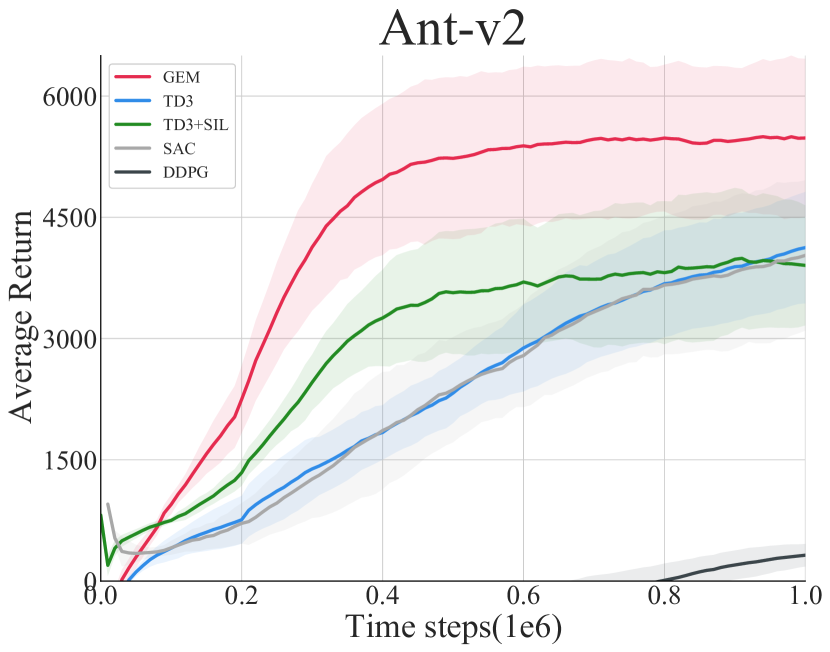
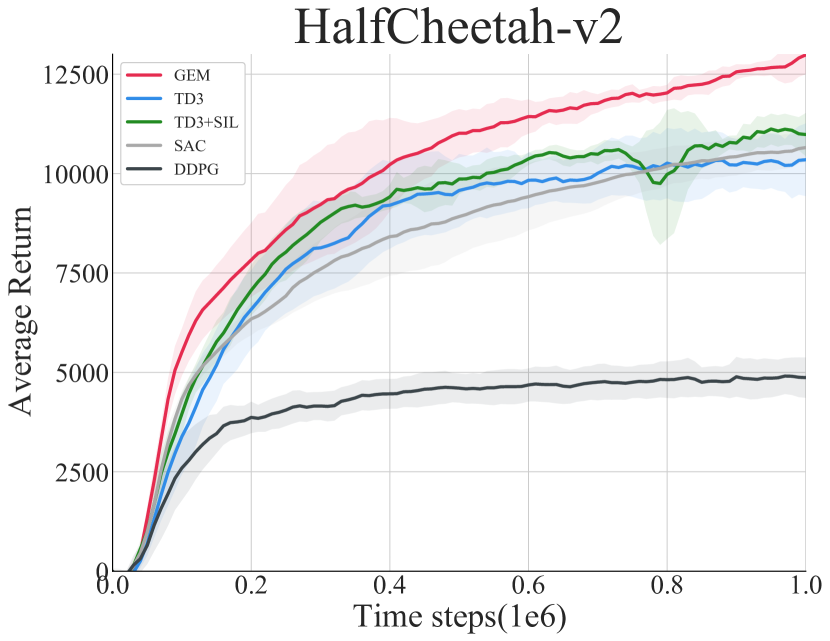
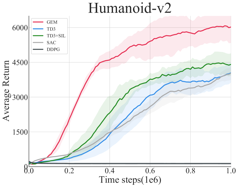
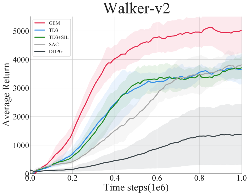
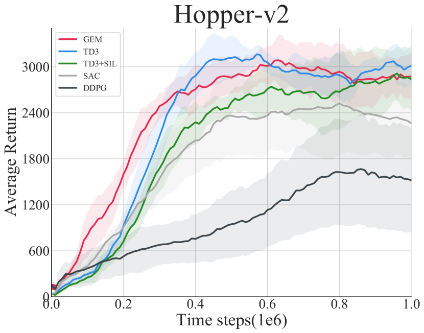
Figure 2: Learning curves on MuJoCo tasks, compared with baseline algorithms. The shaded region represents the standard deviation of the performance. Each curve is averaged over five seeds and is smoothed for visual clarity.

5.1 Evaluation on Continuous Control Tasks

We compare our method with the most popular model-free RL algorithms, including DDPG (Lillicrap et al., 2016), TD3 (Fujimoto et al., 2018) and SAC (Haarnoja et al., 2018). Conventional episodic RL such as MFEC (Blundell et al., 2016), NEC (Pritzel et al., 2017), EMDQN (Lin et al., 2018), EVA (Hansen et al., 2018) and ERLAM (Zhu et al., 2020) adopts discrete episodic memory that are only designed for discrete action space, thus we cannot directly compare with them. To compare with episodic memory-based approaches on the continuous domain, we instead choose self-imitation learning (SIL; Oh et al., 2018) in our experiments. It also aims to exploit past good experiences and share a similar idea with episodic control; thus, it can be regarded as a continuous version of episodic control. For a fair comparison, We use the same code base for all algorithms, and we combine the self-limitation learning objective with techniques in TD3 (Fujimoto et al., 2018), rather than use the origin implementation, which combines with PPO (Schulman et al., 2017).

We conduct experiments on the suite of MuJoCo tasks (Todorov et al., 2012), with OpenAI Gym interface (Brockman et al., 2016). We truncate the maximum steps available for planning to reduce the overestimation bias. The memory update frequency $u$ is set to 100 with a smoothing coefficient $\tau=0.6$. The rest of the hyperparameters are mostly kept the same as in TD3 to ensure a fair comparison. The detailed hyperparameters used are listed in Appendix C.

The learning curve on different continuous tasks is shown in Figure 2. We report the performance of 1M steps, which is evaluated with $10$ rollouts for every $10000$ steps with deterministic policies. As the results suggest, our method significantly outperforms other baseline algorithms on most tasks. Only on Hopper, GEM is not the absolute best, but all the algorithms have similar performance.

5.2 Evaluation on Discrete Domains

Though GEM is proposed to facilitate continuous control tasks, it also has the general applicability of boosting learning on discrete domains. To demonstrate this, we compare GEM with several advanced deep Q-learning algorithms for discrete action space, including DQN (Mnih et al., 2015), DDQN (van Hasselt et al., 2016), and Dueling DQN (Wang et al., 2016). We also include the clipped double DQN, which is adopted from a state-of-the-art algorithm of the continuous domain, TD3 (Fujimoto et al., 2018). Most of these baseline algorithms focus on learning stability and the reduction of estimation bias. We evaluate all the above algorithms on 6 Atari games (Bellemare et al., 2013). We use hyper-parameters suggested in Rainbow (Hessel et al., 2018), and other hyper-parameters for our algorithm are kept the same as in the continuous domain. As shown in Figure 3, although not tailored for the discrete domain, GEM significantly outperforms baseline algorithms both in terms of sample efficiency and final performance.

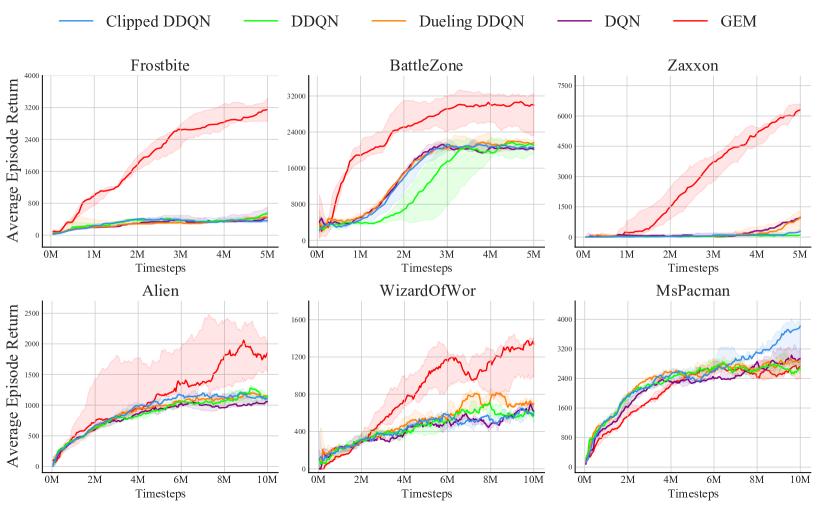
Figure 3: Performance comparison on six Atari games supported by OpenAI gym. Each curve is averaged over three seeds. The shaded region represents the standard deviation of the performance.

5.3 Ablation Study

This section aims to understand each part’s contribution to our proposed algorithm, including the generalizable episodic memory, implicit memory-based planning, and twin back-propagation. We also empirically demonstrate the effect of overestimation. To check whether our method, which uses four networks, benifits from ensembling effect, we also compare our method with the random ensembling method as used in REDQ (Chen et al., 2021).

To verify the effectiveness of generalizable episodic memory, we compare our algorithm with SIL, which directly uses historical returns (which can be seen as a discrete episodic memory). As shown in both Figure 2 and Figure 4, although SIL improves over TD3, it only has marginal improvement. On the contrary, our algorithm improves significantly over TD3.

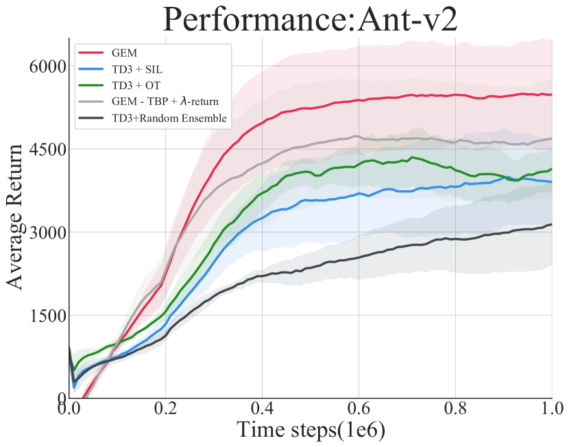
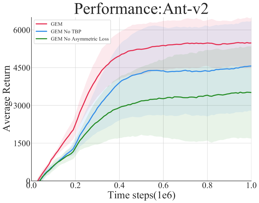
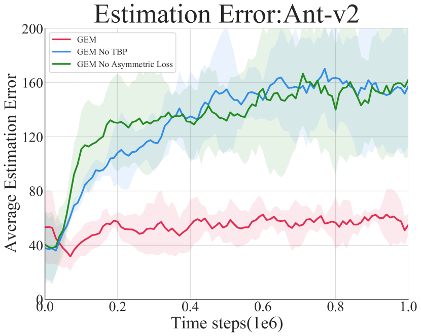
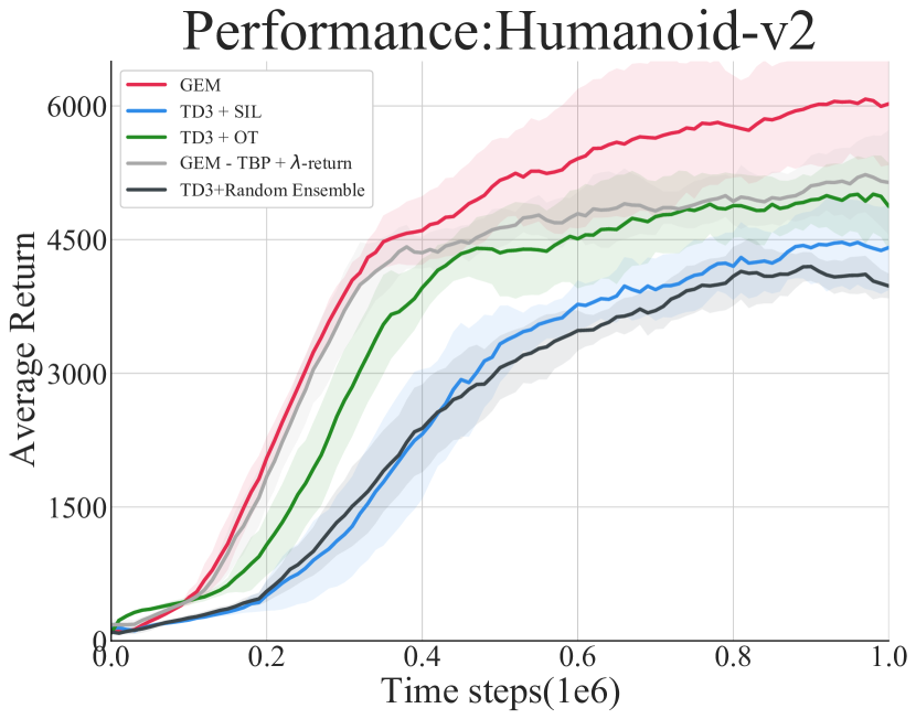
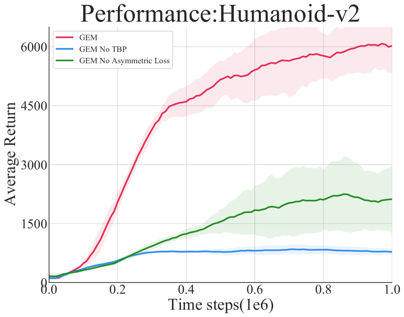
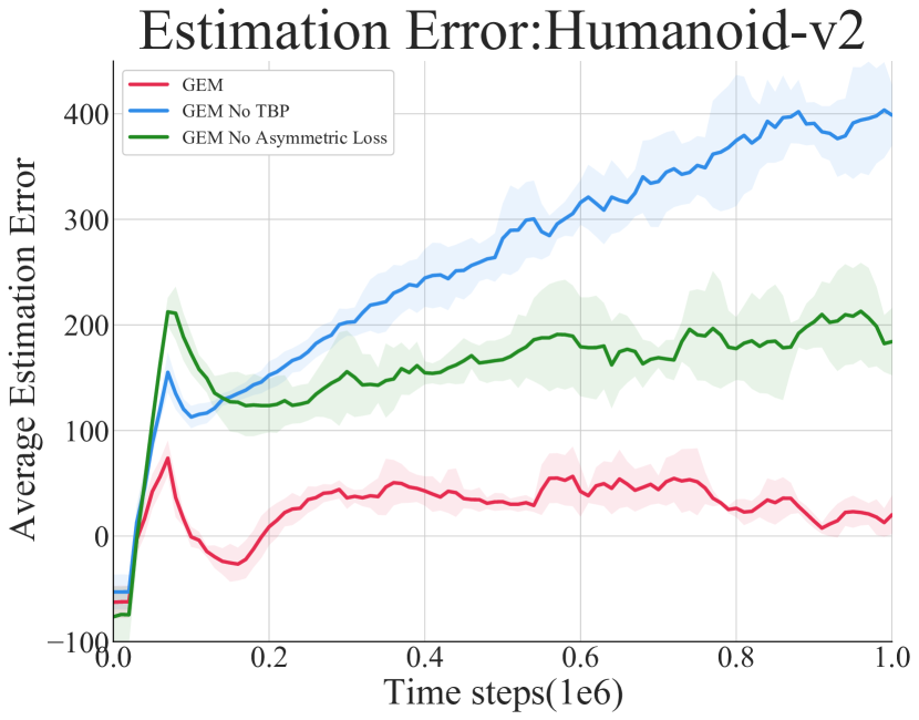
Figure 4: Addtional comparison, ablation study of GEM and empirical evaluation for overestimation. The shaded region represents the standard deviation of the performance. Each curve is averaged over five seeds and is smoothed for visual clarity. Estimation error refers to the average estimated Q-values minus the average returns.

To understand the contribution of implicit planning, we compare with a variant of our method that uses $\lambda$-return rather than taking the maximum over different steps. We also compare our method with Optimality Tightening (He et al., 2017), which shares the similar idea of using trajectory-based information. As Figure 4 shows, Our method outperforms both methods, which verifies the effectiveness of implicit planning within memories.

To check the contribution of our twin network and conservative estimation, we compare the results without the twin back-propagation process and the results without asymmetric losses. The result and the estimation error are summarized in Figure 4. We can see that overestimation is severe without TBP or conservative estimation, and the performance is greatly affected, especially in games like Humanoid. In these games, the living condition for the agent is strict; thus overestimation is more severely punished.

To understand the contribution of the ensembling effect in our method, we compare our result with random ensembling as used in Chen et al. (2021), since we are not able to directly remove TBP while still using all four networks. We use the same update-to-data ratio as in GEM for a fair comparison. As Figure 4 shows, naive ensembling contributes little to performance, and overestimation reduction contributes much more than the ensembling effect.

From these comparisons, we can conclude that our generalizable memory aggregates return values much more effectively than directly using historical returns, and the twin back-propagation process contributes to the performance of GEM significantly. In addition, we verify that the merits of the twin back-propagation process mainly come from overestimation reduction rather than ensembling.

6 Related Work

Episodic Control.

Our method is closely related to episodic reinforcement learning, pioneered by Blundell et al. (2016), which introduces the concept of episodic memory into reinforcement learning and uses a non-parametric k-NN search to recall past successful experiences quickly. Pritzel et al. (2017) and Lin et al. (2018) consider to include a parametric counterpart for episodic memory, which enables better generalizability through function approximators. Although they provide some level of generalization ability, the aggregation of different trajectories still relies on the exact re-encountering, and their methods cannot handle continuous action space. Several advanced variants (Zhu et al., 2020; Lee et al., 2019) propose several ways to connect different experiences within the episodic memory to improve learning speed further. However, their methods are still not generally applicable in the continuous domain since they require taking maximum among all possible actions or require exact re-encountering. Hansen et al. (2018) adopts the similar idea of soft aggregation as ours, but they only consider decision time and leaves the ability of learning by analogy aside. Self-imitation learning (Oh et al., 2018), another memory-based approach built upon policy gradient methods, uses a return-based lower bound to restrict the value function, which cannot aggregate associative trajectories effectively.

From Discrete to Continuous.

Researchers have long been attracted to the challenge of making the RL algorithm applicable in the general continuous case. Kernel-based reinforcement learning (Ormoneit & Sen, 2002) proposes a way to overcomes the stability problems of temporal-difference learning in continuous state-spaces. Lillicrap et al. (2016) extends the success of deep Q-learning into the continuous domain, which successes on various MuJoCo tasks. Similarly, in episodic RL, GEM generalizes the idea of a discrete episodic memory by representing the episodic memory as a network-generated virtual table, making it generally applicable in the continuous case.

Maximization Bias in Q-Learning.

The maximization bias of Q-learning, first highlighted by Thrun & Schwartz (1993), is a long-lasting issue that hinders the learning efficiency of value-based methods. van Hasselt (2010) proposed to use a second value estimator as cross-validation to address this bias, and this technique has been extended to the deep Q-learning paradigm (van Hasselt et al., 2016). In practice, since it is intractable to construct two fully independent value estimators, double Q-learning is observed to overestimate sometimes, especially in continuous domains. To address this concern, Fujimoto et al. (2018) proposed clipped double Q-learning to repress further the incentive of overestimation, which has become the default implementation of most advanced approaches (Haarnoja et al., 2018; Kalashnikov et al., 2018). Recently, to control the estimation bias more precisely, people utilize an ensemble of value networks (Lan et al., 2020; Kuznetsov et al., 2020; Chen et al., 2021), which causes high computational costs.

Multi-step Bootstrapping.

The implementation of our proposed algorithm is also related to a technique named multi-step bootstrapping. This branch originates from the idea of eligibility traces (Singh & Sutton, 1996; Sutton, 1988b). Recently, it is prevalent in policy gradient methods such as GAE (Schulman et al., 2016) and its variants (Touati et al., 2018). In the context of temporal-difference learning, multi-step bootstrapping is also beneficial to improving the stability of Q-learning algorithms (Van Hasselt et al., 2018). The main limitation of multi-step bootstrapping is that the performance of multi-step training is sensitive to the bootstrapping horizon choice, and the trajectory used is required to be at least nearly on-policy rather than an arbitrary one.

7 Conclusion

This work presents Generalizable Episodic Memory, an effective memory-based method that aggregates different experiences from similar states and future consequences. We perform implicit planning by taking the maximum over all possible combinatorial trajectories in the memory and reduces overestimation error by using twin networks.

We provide theoretical analysis to show that our objective does not overestimate in general and converges to $Q^{*}$ under mild conditions. Experimental results on continuous control tasks show that our method outperforms state-of-the-art model-free RL methods, as well as episodic memory-based algorithms. Our method also demonstrates general applicability in the discrete domain, such as Atari games. Our method is not primarily designed for discrete domains but can still significantly improve the learning efficiency of RL agents under this setting.

We make the first step to endow episodic memory with generalization ability. Besides, generalization ability also relies highly on the representation of states and actions. We leave the study of representation learning in episodic memory as interesting future work.

8 Acknowledgement

This work is supported in part by Science and Technology Innovation 2030 – “New Generation Artificial Intelligence” Major Project (No. 2018AAA0100904), and a grant from the Institute of Guo Qiang,Tsinghua University.

Appendix A GEM Algorithm in Tabular Case

In this section, we present the formal description of the GEM algorithm in tabular case, as shown in Algorithm 3.

Algorithm 3 Generalizable Episodic Memory in Tabular Case

  Initialize table $Q^{(1)}(s,a),Q^{(2)}(s,a)$ arbitrarily,

  Initial learning step size $\alpha_{t}$, small $\epsilon>0$ and episode length $l=0$

  Set $\pi$ to be the $\epsilon$-greedy policy with respect to $Q^{(1)}(s,a)$ or $Q^{(2)}(s,a)$

  for $t=1,\cdots,$ do

     Initialize and store $s_{0}$

     Select action $a_{0}\sim\pi(\cdot|s_{0})$ 

     Observe reward $r$ and new state $s^{\prime}$ 

     Store transition tuple $(s,a,r,s^{\prime})$ 

     $l\leftarrow l+1$

     if  an episode is ended then

        for  $\tau=t-l,\cdots,t$  do

           Compute $R^{(1)}_{\tau},R^{(2)}_{\tau}$ according to Equation (7) 

           Uniformly choose $i\in\{1,2\}$ 

           Update $Q^{(i)}(s_{\tau},a_{\tau})\leftarrow Q^{(i)}(s_{\tau},a_{\tau})+\alpha_{\tau}(R_{\tau}^{(i)}-Q^{(i)}(s_{\tau},a_{\tau}))$ 

        end for

        Set $\pi$ to be the $\epsilon$-greedy policy with respect to $Q^{(1)}(s,a)$ or $Q^{(2)}(s,a)$

        $l\leftarrow 0$

     end if

  end for

Appendix B Proofs of Theoremss

Theorem 4.

Given unbiased and independent estimators $Q^{(1,2)}_{\theta}(s_{t+h},a_{t+h})=Q^{\pi}(s_{t+h},a_{t+h})+\epsilon^{(1,2)}_{h}$, Equation (8) will not overestimate the true objective, i.e.

$$\operatorname{\mathbb{E}}_{\tau,\epsilon}\left[R_{t}^{(1,2)}(s_{t})\right]\leq\operatorname{\mathbb{E}}_{\tau}\left[\max_{0\leq h\leq T-t-1}Q^{\pi}_{t,h}(s_{t})\right],$$ (13)

where

$$Q^{\pi}_{t,h}(s,a)=\left\{\begin{aligned} &\sum_{i=0}^{h}\gamma^{i}r_{t+i}+\gamma^{h+1}Q^{\pi}(s_{t+h+1},a_{t+h+1})&\text{if }h<T-t,\\ &\sum_{i=0}^{h}\gamma^{i}r_{t+i}&\text{if }h=T-t.\end{aligned}\right.$$ (14)

and $\tau=\{(s_{t},a_{t},r_{t},s_{t+1})_{t=1,\cdots,T}\}$ is a trajectory.

Proof.

By unrolling and rewritten Equation (7), we have

$$R_{t}^{(1,2)}=V_{t,h^{*}}=\sum_{i=0}^{h^{*}}\gamma^{i}r_{t+i}+\gamma^{h^{*}+1}Q^{(2,1)}_{\theta}(s_{t+h^{*}+1},a_{t+h^{*}+1}),$$

Where $h^{*}$ is the abbrevation for $h^{*}_{(1,2)}$ for simplicity. Then we have

$$\operatorname{\mathbb{E}}_{\epsilon}\left[R_{t}^{(1,2)}-Q^{\pi}_{t,h^{*}_{(1,2)}}(s_{t})\right] =\operatorname{\mathbb{E}}\left[V_{t,h^{*}_{(1,2)}}-Q^{\pi}_{t,h^{*}_{(1,2)}}(s_{t})\right]$$

$$=\operatorname{\mathbb{E}}\left[\gamma^{h^{*}+1}\left(Q^{(2,1)}_{\theta}(s_{t+h^{*}+1},a_{t+h^{*}+1})-Q^{\pi}(s_{t+h^{*}+1},a_{t+h^{*}+1})\right)\right]$$

$$=0.$$

Then naturally

$$\operatorname{\mathbb{E}}_{\tau,\epsilon}[R_{t}^{(1,2)}]=\operatorname{\mathbb{E}}_{\tau}[Q^{\pi}_{t,h^{*}_{(1,2)}}(s_{t})]\leq\operatorname{\mathbb{E}}_{\tau}\left[\max_{0\leq h\leq T-t}{Q^{\pi}_{t,h}(s_{t})}\right].$$

∎

To prepare for the theorem below, we need the following lemma:

Lemma 2.

Consider a stochastic process $(\zeta_{t},\Delta_{t},F_{t}),t\geq 0$, where $\zeta,\Delta_{t},F_{t}:X\rightarrow\mathbb{R}$ satisfy the equations

$$\Delta_{t+1}(x)=(1-\zeta_{t}(x))\Delta_{t}(x)+\zeta_{t}(x)F_{t}(x)$$ (15)

Let $\{P_{t}\}$ be a filter such that $\zeta_{t}$ and $\Delta_{t}$ are $P_{t}$-measurable, $F_{t}$ is $P_{t+1}$-measurable, $t\geq 0$. Assume that the following hold:

• $X$ is finite: $|X|<+\infty$.

• $\zeta_{t}(x)\in[0,1]$, $\sum_{t}\zeta_{t}(x)=+\infty$, $\sum_{t}\zeta_{t}^{2}(x)<+\infty$ a.s. for all $x\in X$.

• $\|\mathbb{E}(F_{t}|P_{t})\|_{\infty}\leq\kappa\|\Delta_{t}\|_{\infty}+c_{t}$, where $\kappa\in[0,1)$ and $c_{t}\stackrel{{\scriptstyle\text{a.s}}}{{\rightarrow}}0$.

• $\text{Var}(F_{t}|P_{t})\leq K(1+\|\Delta_{t}\|_{\infty})^{2}$, where $K$ is some constant.

Then $\Delta_{t}$ converge to zero w.p.1.

This lemma is also used in Double-Q learning (van Hasselt, 2010) and we omit the proof for simplicity.
In the following sections, we use $\left\lVert\cdot\right\rVert$ to represent the infinity norm $\left\lVert\cdot\right\rVert_{\infty}$.

Theorem 5.

Algorithm 3 converge to $Q^{*}$ w.p.1 with the following conditions:

1. The MDP is finite, i.e. $|\mathcal{S}\times\mathcal{A}|\leq\infty$

2. $\gamma\in[0,1)$

3. The Q-values are stored in a lookup table

4. $\alpha_{t}(s,a)\in[0,1],\sum_{t}{\alpha_{t}(s,a)}=\infty,\sum_{t}{\alpha_{t}^{2}(s,a)}\leq\infty$

5. The environment is fully deterministic, i.e. $P(s^{\prime}|s,a)=\delta(s^{\prime}=f(s,a))$ for some deterministic transition function $f$

Proof.

This is a sketch of proof and some technical details are omitted.

We just need to show that without double-q version, the update will be a $\gamma$-contraction and will converge. Then we need to show that $\left\lVert Q^{1}-Q^{2}\right\rVert$ converge to zero, which is similar with double-q learning.

We only prove convergence of $Q^{(1)}$, and by symmetry we have the conclusion.

Let $\Delta_{t}=Q_{t}^{(1)}-Q^{*}$, and $F_{t}(s_{t},a_{t})=R^{(1)}_{t}-Q^{*}(s_{t},a_{t})$,

Then the update rule can be written exactly as Equation (15):

$$\Delta_{t+1}=(1-\alpha_{t})\Delta_{t}+\alpha_{t}F_{t}.$$

We define

$$G_{t}=\tilde{R}^{(1)}_{t}-Q^{*}(s_{t},a_{t})=F_{t}+(\tilde{R}^{(1)}_{t}-R^{(1)}_{t}),$$

where $\tilde{R}^{(1)}=R^{(1)}_{t,h^{*}_{(1)}},$and the notation is kept the same as in Equation (7) & (8).

To use Lemma 2, we only need to prove that $G_{t}$ is a $\gamma$-contraction and $c_{t}=\tilde{R}^{(1)}_{t}-R^{(1)}_{t}$ converge to zero.

On the one hand,

$$\tilde{R}^{(1)}_{t}-Q^{*}(s_{t},a_{t}) \geq r_{t}+\gamma\tilde{Q}^{(1)}(s_{t+1},\tilde{a}^{*})-Q^{*}(s_{t},a_{t})$$

$$=r_{t}+\gamma\tilde{Q}^{(1)}(s_{t+1},\tilde{a}^{*})-r_{t}+\gamma Q^{*}(s_{t+1},a^{*})$$

$$=\gamma(\tilde{Q}^{(1)}(s_{t+1},\tilde{a}^{*})-Q^{*}(s_{t+1},a^{*}))$$

$$\geq-\gamma\left\lVert\Delta_{t}\right\rVert.$$

On the other hand,

$$\tilde{R}^{(1)}_{t}-Q^{*}(s_{t},a_{t}) =\sum_{i=0}^{h^{*}_{(1)}}\gamma^{i}r_{t+i}+\gamma^{h^{*}_{(1)}+1}\tilde{Q}^{(1)}(s_{t+h^{*}_{(1)}+1},\tilde{a}^{*})-Q^{*}(s_{t},a_{t})$$

$$\leq\sum_{i=0}^{h^{*}_{(1)}}\gamma^{i}r_{t+i}+\gamma^{h^{*}_{(1)}+1}\tilde{Q}^{(1)}_{\pi}(s_{t+h^{*}_{(1)}+1})$$

$$-(\sum_{i=0}^{h^{*}_{(1)}}\gamma^{i}r_{t+i}+\gamma^{h^{*}_{(1)}+1}Q^{*}(s_{t+h^{*}_{(1)}+1},a^{*}))$$

$$=\gamma^{h^{*}_{(1)}+1}(\tilde{Q}^{(1)}(s_{t+h^{*}_{(1)}+1},\tilde{a}^{*})-Q^{*}(s_{t+h^{*}_{(1)}+1},a^{*}))$$

$$\leq\gamma(\tilde{Q}^{(1)}(s_{t+h^{*}_{(1)}+1},\tilde{a}^{*})-Q^{*}(s_{t+h^{*}_{(1)}+1},a^{*}))$$

$$\leq\gamma\left\lVert\Delta_{t}\right\rVert.$$

Thus $G_{t}$ is a $\gamma$-contraction w.r.t $\Delta_{t}$.

Finally we show $c_{t}=\tilde{R}^{(1)}-R^{(1)}_{t}$ converges to zero.

Note that $c_{t}=\gamma^{h^{*}_{(1)}}(\tilde{Q}^{(1)}-\tilde{Q}^{(2)})$, it suffices to show that $\Delta^{1,2}=\tilde{Q}^{(1)}-\tilde{Q}^{(2)}$ converge to zero.

Depending on whether $\tilde{Q}^{(1)}$ or $\tilde{Q}^{(2)}$ is updated, the update rule can be written as

$$\Delta^{1,2}_{t+1}=\Delta^{1,2}_{t}+\alpha_{t}F_{t}^{(2)}(s_{t},a_{t}),$$

or

$$\Delta^{1,2}_{t+1}=\Delta^{1,2}_{t}-\alpha_{t}F_{t}^{(1)}(s_{t},a_{t}),$$

where $F_{t}^{(1)}=R_{t}^{(1)}-\tilde{Q}_{t}^{(2)}$ and $F_{t}^{(2)}=R_{t}^{(2)}-\tilde{Q}_{t}^{(1)}$.

Now let $\zeta_{t}=\frac{1}{2}\alpha_{t}$, we have

$$\operatorname{\mathbb{E}}[\Delta^{1,2}_{t+1}|P_{t}] =\frac{1}{2}(\Delta^{1,2}+\alpha_{t}\operatorname{\mathbb{E}}[F_{t}^{(2)}])+\frac{1}{2}(\Delta^{1,2}-\alpha_{t}\operatorname{\mathbb{E}}[F_{t}^{(1)}])$$

$$=(1-\zeta_{t})\Delta^{1,2}_{t}+\zeta_{t}\operatorname{\mathbb{E}}[R_{t}^{(2)}-R_{t}^{(1)}]$$

when $\operatorname{\mathbb{E}}[R_{t}^{(2)}]\geq\operatorname{\mathbb{E}}[R_{t}^{(1)}],$ by definition we have $\operatorname{\mathbb{E}}[R_{t}^{(2)}]\leq\operatorname{\mathbb{E}}[\tilde{R}_{t}^{(2)}].$

Then

$$|\operatorname{\mathbb{E}}[R_{t}^{(2)}-R_{t}^{(1)}]| \leq\operatorname{\mathbb{E}}[\tilde{R}_{t}^{(2)}-R_{t}^{(1)}]$$

$$\leq\gamma^{h^{*}_{(2)}+1}(Q^{(1)}(s_{t+h^{*}_{(2)}+1},a^{*}_{(1)})-Q^{(2)}(s_{t+h^{*}_{(2)}+1},a^{*}_{(1)}))$$

$$\leq\gamma\left\lVert\Delta^{1,2}_{t}\right\rVert.$$

Similarly, $\operatorname{\mathbb{E}}[R_{t}^{(2)}]<\operatorname{\mathbb{E}}[R_{t}^{(1)}],$, we have

$$|\operatorname{\mathbb{E}}[R_{t}^{(2)}-R_{t}^{(1)}]| \leq\operatorname{\mathbb{E}}[\tilde{R}_{t}^{(1)}-R_{t}^{(2)}]$$

$$\leq\gamma^{h^{*}_{(1)}+1}(Q^{(2)}(s_{t+h^{*}_{(1)}+1},a^{*}_{(2)})-Q^{(1)}(s_{t+h^{*}_{(1)}+1},a^{*}_{(2)}))$$

$$\leq\gamma\left\lVert\Delta^{1,2}_{t}\right\rVert.$$

Now in both scenairos we have $|E\{F^{(1,2)}_{t}|P_{t}\}|\leq\gamma\left\lVert\Delta^{1,2}_{t}\right\rVert$ holds. Applying Lemma 2 again we have the desired results. ∎

The theorem apply only to deterministic scenairos. Nevertheless, we can still bound the performance when the environment is stochastic but nearly deterministic.

Theorem 6.

$\tilde{Q}(s,a)$ learned by Algorithm 3 satisfy the following inequality:

$$\forall s\in\mathcal{S},a\in\mathcal{A},Q^{*}(s,a)\leq\tilde{Q}(s,a)\leq Q_{\text{max}}(s,a),$$ (16)

w.p.1 with condition 1-4 in Theorem 2.

Proof.

We just need to prove that $(Q^{*}-Q^{(1,2)})_{+}$ and $(Q^{(1,2)}-Q_{\text{max}})_{+}$ converge to 0 w.p.1, where $(\cdot)_{+}=\max(0,\cdot)$.

On the one hand, similar from the proof of Theorem 2 and let $\Delta_{t}=(Q^{*}(s_{t},a_{t})-Q^{(1,2)}(s_{t},a_{t}))_{+}$.

$$Q^{*}(s_{t},a_{t})-\tilde{R}^{(1,2)}_{t} \leq Q^{*}(s_{t},a_{t})-(r_{t}+\gamma\tilde{Q}^{(1,2)}(s_{t+1},\tilde{a}^{*}))$$

$$=r_{t}+\gamma Q^{*}(s_{t+1},a^{*})-r_{t}-\gamma\tilde{Q}^{(1,2)}(s_{t+1},\tilde{a}^{*})$$

$$=\gamma(\tilde{Q}(s_{t+1},\tilde{a}^{*})-Q^{*}(s_{t+1},a^{*}))$$

$$\leq\gamma\left\lVert\Delta_{t}\right\rVert.$$

The rest is the same as the proof of Theorem 2, and we have $(Q^{*}-Q^{(1,2)})_{+}$ converge to zero w.p.1.

On the other hand, let $\Delta_{t}=(Q_{\text{max}}(s_{t},a_{t})-Q^{(1,2)}(s_{t},a_{t}))_{+}$,

We have

$$F_{t+1} =\tilde{R}^{(1,2)}_{t}-Q^{max}_{t}$$

$$\leq\sum^{h^{*}_{(2,1)}}_{i=0}\gamma^{i}r_{t+i}+\gamma^{h^{*}+1}\tilde{Q}^{(1,2)}_{t+h^{*}_{(2,1)+1}}-(\sum^{h^{*}_{(2,1)}}_{i=0}\gamma^{i}r_{t+i}+\gamma^{h^{*}+1}Q^{max}_{t+h^{*}_{(2,1)+1}})$$

$$\leq\gamma^{h^{*}+1}(\tilde{Q}^{(1,2)}_{t+h^{*}_{(2,1)+1}}-Q^{max}_{t+h^{*}_{(2,1)+1}})$$

$$\leq\gamma\left\lVert\Delta_{t}\right\rVert.$$

The rest is the same as the proof of Theorem 2, and we have $(Q^{(1,2)}-Q_{\text{max}})_{+}$ converge to zero w.p.1.

∎

When the enironment is nearly-deterministic, we can bound the performance of Q despite its non-convergence:

Theorem 7.

For a nearly-deterministic environment with factor $\mu$, in limit, GEM’s performance can be bounded by

$$V^{\tilde{\pi}}(s)\geq V^{*}(s)-\frac{2\mu}{1-\gamma},\forall s\in\mathcal{S}.$$ (17)

Proof.

since we have $\left\lVert\tilde{Q}-Q^{*}\right\rVert\leq\mu$, It is easy to show that

$$V^{*}(s)-V^{\tilde{\pi}}(s)$$

$$=Q^{*}(s,a^{*})-Q^{\tilde{\pi}}(s,\tilde{a})$$

$$=Q^{*}(s,a^{*})-\tilde{Q}(s,a^{*})+\tilde{Q}(s,a^{*})-Q^{\tilde{\pi}}(s,\tilde{a})$$

$$\leq\epsilon+\tilde{Q}(s,\tilde{a})-Q^{\tilde{\pi}}(s,\tilde{a})$$

$$=\epsilon+(\tilde{Q}(s,\tilde{a})-Q^{*}(s,\tilde{a}))+(Q^{*}(s,\tilde{a})-Q^{\tilde{\pi}}(s,\tilde{a}))$$

$$\leq 2\epsilon+\gamma(V^{*}(s)-V^{\tilde{\pi}}(s)).$$

So we have the conclusion. ∎

Appendix C Hyperparameters

Here we listed the hyperparameters we used for the evaluation of our algorithm.

Task	HalfCheetah	Ant	Swimmer	Humanoid	Walker	Hopper
Maximum Length $d$	1000	1000	1000	5	5	5

Table 1: Maximum length of rollouts used in GEM across different tasks

Hyper-parameter	GEM
Critic Learning Rate	1e-3
Actor Learning Rate	1e-3
Optimizer	Adam
Target Update Rate($\tau$)	0.6
Memory Update Period($u$)	100
Memory Size	100000
Policy Delay($p$)	2
Batch Size	100
Discount Factor	0.99
Exploration Policy	$\mathcal{N}(0,0.1)$
Gradient Steps per Update	200

Table 2: List of Hyperparameters used in GEM across different tasks

The hyper-parameters for Atari games are kept the same as in the continuous domain, and other hyper-parameters are kept the same as Rainbow (Hessel et al., 2018).

Appendix D Additional Ablation Results

Here we include more ablation results of GEM. To verify the effectiveness of our proposed implicit planning, we compare our method with simple n-step Q learning combined with TD3. For a fair comparison, we include all different rollout lengths used in GEM’s result. The result is shown in Figure 6. We can see that GEM significantly outperform simple n-step learning.

To understand the effects of rollout lengths, we also compare the result of different rollout lengths on Atari games. The result is shown below in Figure 7. We can see that using short rollout length greatly hinders the performance of GEM.

To verify the effectiveness of GEM on the stochastic domain, we conduct experiments on Atari games with sticky actions, as suggested in (Machado et al., 2018). As illustrated in Figure 5, GEM is still competitive on stochastic domains.

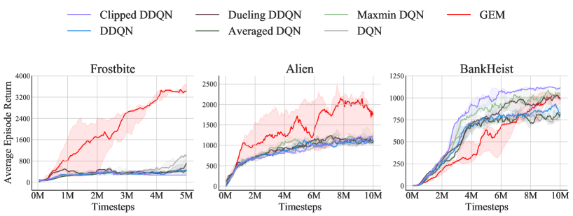
Figure 5: Comparison on 3 Atari games, with sticky actions to make the environment stochastic.

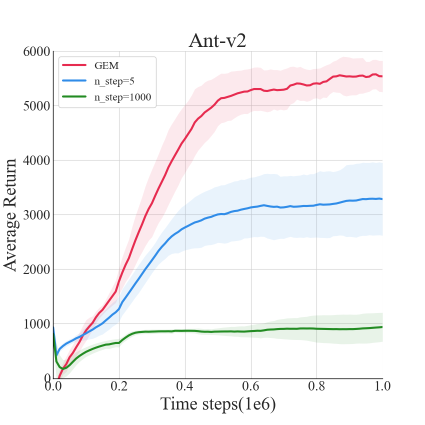
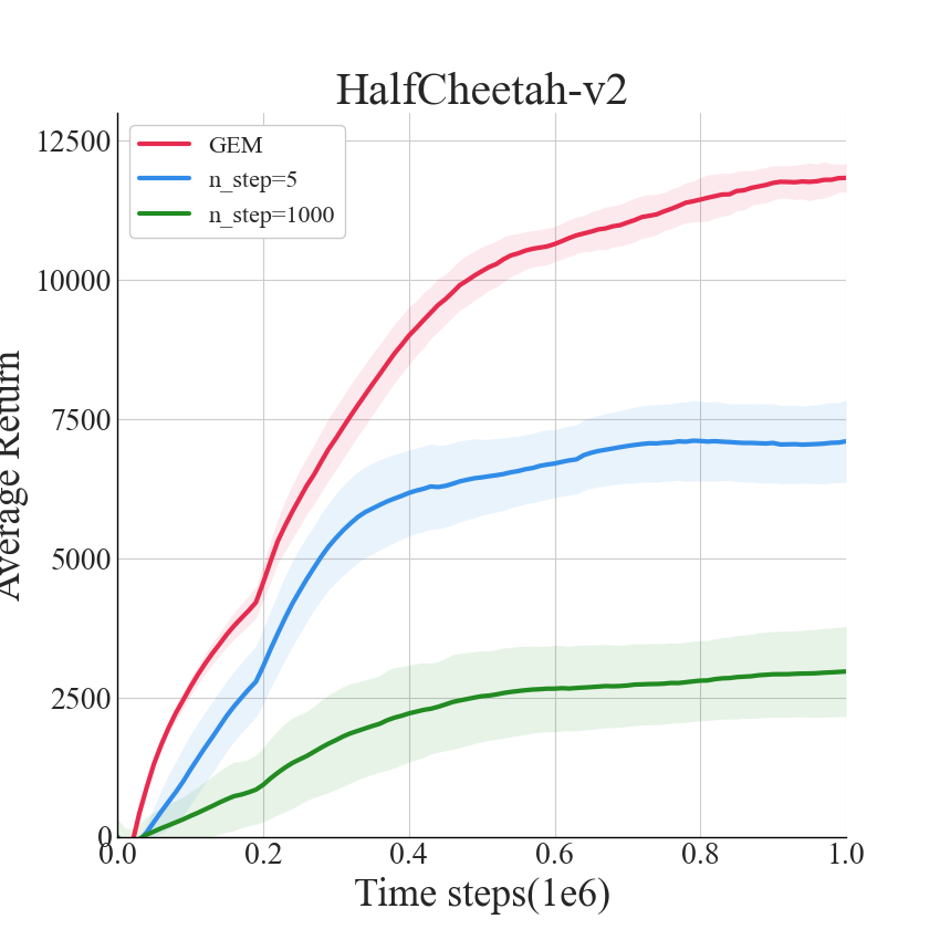
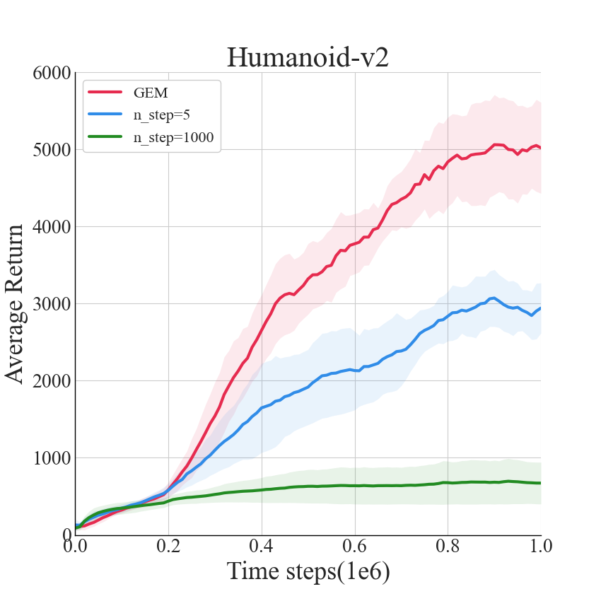
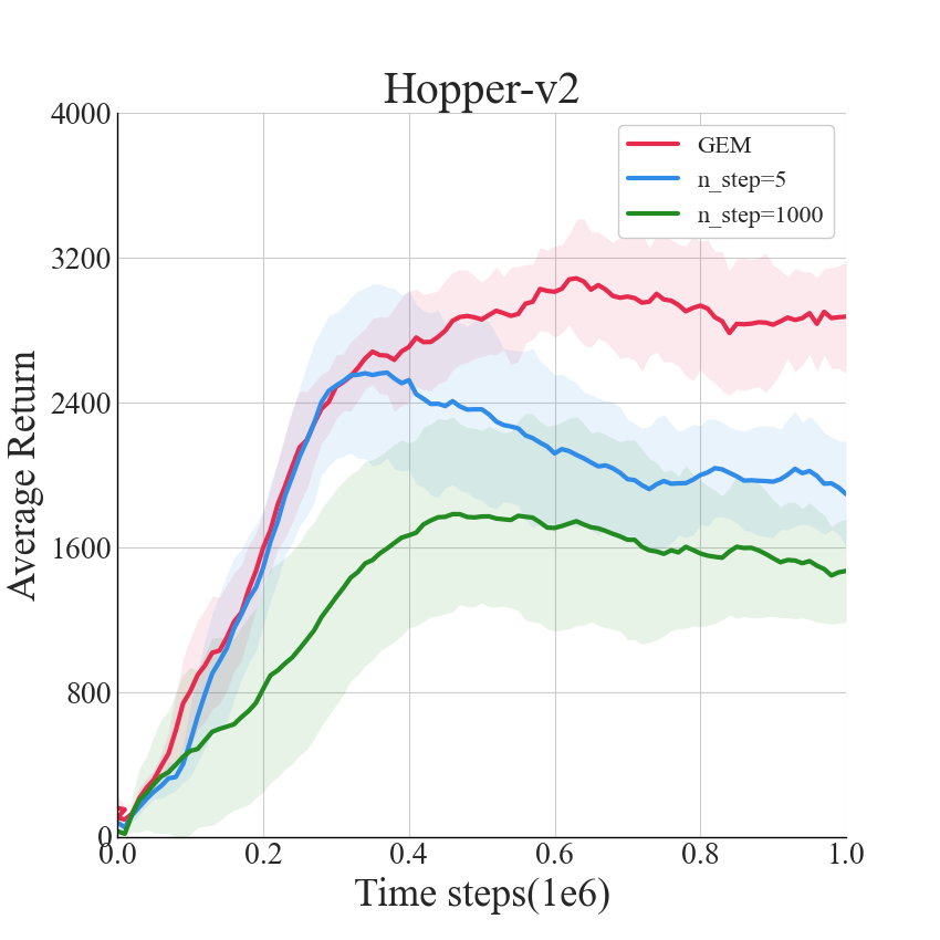
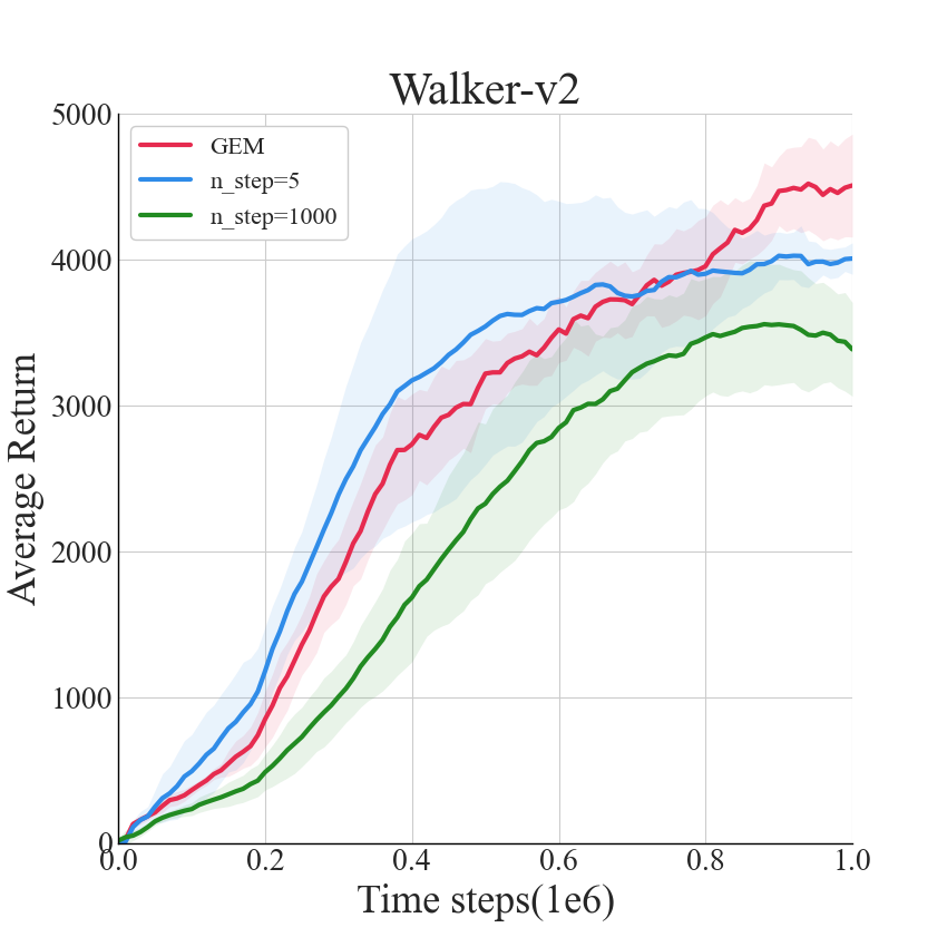
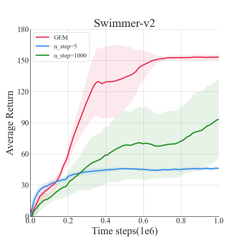
Figure 6: Comparison with simple n-step learning. The shaded region represents half a standard deviation of the average evaluation. Curves are smoothed uniformly for visual clarity.

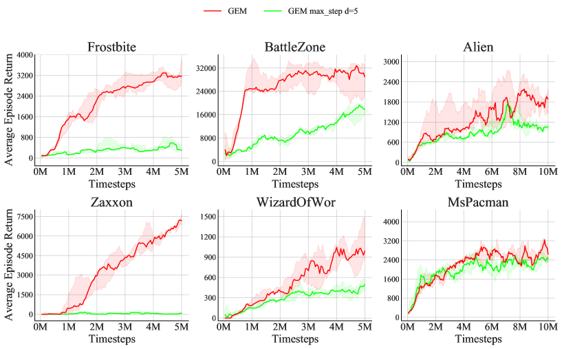
Figure 7: Ablation study on 6 Atari games. Limiting rollout lengths greatly affects the performance of GEM, which proves that GEM can use long rollout trajectories effectively.

References

- Bellemare et al. (2013) Bellemare, M. G., Naddaf, Y., Veness, J., and Bowling, M. The arcade learning environment: An evaluation platform for general agents. Journal of Artificial Intelligence Research, 47:253–279, 2013.
- Bellman (1957) Bellman, R. Dynamic programming princeton university press princeton. New Jersey Google Scholar, 1957.
- Blundell et al. (2016) Blundell, C., Uria, B., Pritzel, A., Li, Y., Ruderman, A., Leibo, J. Z., Rae, J., Wierstra, D., and Hassabis, D. Model-free episodic control. arXiv preprint arXiv:1606.04460, 2016.
- Botvinick et al. (2019) Botvinick, M., Ritter, S., Wang, J. X., Kurth-Nelson, Z., Blundell, C., and Hassabis, D. Reinforcement learning, fast and slow. Trends in cognitive sciences, 23(5):408–422, 2019.
- Brockman et al. (2016) Brockman, G., Cheung, V., Pettersson, L., Schneider, J., Schulman, J., Tang, J., and Zaremba, W. Openai gym. arXiv preprint arXiv:1606.01540, 2016.
- Chen et al. (2021) Chen, X., Wang, C., Zhou, Z., and Ross, K. Randomized ensembled double q-learning: Learning fast without a model. In International Conference on Learning Representations, 2021.
- Fujimoto et al. (2018) Fujimoto, S., van Hoof, H., and Meger, D. Addressing function approximation error in actor-critic methods. In Dy, J. G. and Krause, A. (eds.), Proceedings of the 35th International Conference on Machine Learning, ICML 2018, volume 80 of Proceedings of Machine Learning Research, pp. 1582–1591. PMLR, 2018.
- Gilboa & Schmeidler (1995) Gilboa, I. and Schmeidler, D. Case-based decision theory. The Quarterly Journal of Economics, 110(3):605–639, 1995.
- Haarnoja et al. (2018) Haarnoja, T., Zhou, A., Abbeel, P., and Levine, S. Soft actor-critic: Off-policy maximum entropy deep reinforcement learning with a stochastic actor. In Dy, J. G. and Krause, A. (eds.), Proceedings of the 35th International Conference on Machine Learning, ICML 2018, volume 80 of Proceedings of Machine Learning Research, pp. 1856–1865. PMLR, 2018.
- Hansen et al. (2018) Hansen, S., Pritzel, A., Sprechmann, P., Barreto, A., and Blundell, C. Fast deep reinforcement learning using online adjustments from the past. In Bengio, S., Wallach, H. M., Larochelle, H., Grauman, K., Cesa-Bianchi, N., and Garnett, R. (eds.), Advances in Neural Information Processing Systems 31: Annual Conference on Neural Information Processing Systems 2018, NeurIPS 2018, pp. 10590–10600, 2018.
- He et al. (2017) He, F. S., Liu, Y., Schwing, A. G., and Peng, J. Learning to play in a day: Faster deep reinforcement learning by optimality tightening. In 5th International Conference on Learning Representations, ICLR 2017. OpenReview.net, 2017.
- Hessel et al. (2018) Hessel, M., Modayil, J., van Hasselt, H., Schaul, T., Ostrovski, G., Dabney, W., Horgan, D., Piot, B., Azar, M. G., and Silver, D. Rainbow: Combining improvements in deep reinforcement learning. In McIlraith, S. A. and Weinberger, K. Q. (eds.), Proceedings of the Thirty-Second AAAI Conference on Artificial Intelligence, (AAAI-18), pp. 3215–3222. AAAI Press, 2018.
- Kahn et al. (1981) Kahn, C. H. et al. The art and thought of Heraclitus: a new arrangement and translation of the Fragments with literary and philosophical commentary. Cambridge University Press, 1981.
- Kalashnikov et al. (2018) Kalashnikov, D., Irpan, A., Pastor, P., Ibarz, J., Herzog, A., Jang, E., Quillen, D., Holly, E., Kalakrishnan, M., Vanhoucke, V., et al. Qt-opt: Scalable deep reinforcement learning for vision-based robotic manipulation. In Conference on Robot Learning. PMLR, 2018.
- Kuznetsov et al. (2020) Kuznetsov, A., Shvechikov, P., Grishin, A., and Vetrov, D. P. Controlling overestimation bias with truncated mixture of continuous distributional quantile critics. In Proceedings of the 37th International Conference on Machine Learning, ICML 2020, volume 119 of Proceedings of Machine Learning Research, pp. 5556–5566. PMLR, 2020.
- Lan et al. (2020) Lan, Q., Pan, Y., Fyshe, A., and White, M. Maxmin q-learning: Controlling the estimation bias of q-learning. In 8th International Conference on Learning Representations, ICLR 2020. OpenReview.net, 2020.
- Lee et al. (2019) Lee, S. Y., Choi, S., and Chung, S. Sample-efficient deep reinforcement learning via episodic backward update. In Wallach, H. M., Larochelle, H., Beygelzimer, A., d’Alché-Buc, F., Fox, E. B., and Garnett, R. (eds.), Advances in Neural Information Processing Systems 32: Annual Conference on Neural Information Processing Systems 2019, NeurIPS 2019, pp. 2110–2119, 2019.
- Lengyel & Dayan (2007) Lengyel, M. and Dayan, P. Hippocampal contributions to control: The third way. In Platt, J. C., Koller, D., Singer, Y., and Roweis, S. T. (eds.), Advances in Neural Information Processing Systems 20, Proceedings of the Twenty-First Annual Conference on Neural Information Processing Systems, pp. 889–896. Curran Associates, Inc., 2007.
- Lillicrap et al. (2016) Lillicrap, T. P., Hunt, J. J., Pritzel, A., Heess, N., Erez, T., Tassa, Y., Silver, D., and Wierstra, D. Continuous control with deep reinforcement learning. In Bengio, Y. and LeCun, Y. (eds.), 4th International Conference on Learning Representations, ICLR 2016,, 2016.
- Lin et al. (2018) Lin, Z., Zhao, T., Yang, G., and Zhang, L. Episodic memory deep q-networks. In Lang, J. (ed.), Proceedings of the Twenty-Seventh International Joint Conference on Artificial Intelligence, IJCAI 2018, pp. 2433–2439. ijcai.org, 2018. doi: 10.24963/ijcai.2018/337.
- Machado et al. (2018) Machado, M. C., Bellemare, M. G., Talvitie, E., Veness, J., Hausknecht, M., and Bowling, M. Revisiting the arcade learning environment: Evaluation protocols and open problems for general agents. Journal of Artificial Intelligence Research, 61:523–562, 2018.
- Marr et al. (1991) Marr, D., Willshaw, D., and McNaughton, B. Simple memory: a theory for archicortex. In From the Retina to the Neocortex, pp. 59–128. Springer, 1991.
- Mnih et al. (2015) Mnih, V., Kavukcuoglu, K., Silver, D., Rusu, A. A., Veness, J., Bellemare, M. G., Graves, A., Riedmiller, M., Fidjeland, A. K., Ostrovski, G., et al. Human-level control through deep reinforcement learning. nature, 518(7540):529–533, 2015.
- Oh et al. (2018) Oh, J., Guo, Y., Singh, S., and Lee, H. Self-imitation learning. In Dy, J. G. and Krause, A. (eds.), Proceedings of the 35th International Conference on Machine Learning, ICML 2018, volume 80 of Proceedings of Machine Learning Research, pp. 3875–3884. PMLR, 2018.
- Ormoneit & Sen (2002) Ormoneit, D. and Sen, Ś. Kernel-based reinforcement learning. Machine learning, 49(2):161–178, 2002.
- Peters & Bagnell (2010) Peters, J. and Bagnell, J. A. Policy gradient methods. Scholarpedia, 5(11):3698, 2010.
- Pritzel et al. (2017) Pritzel, A., Uria, B., Srinivasan, S., Badia, A. P., Vinyals, O., Hassabis, D., Wierstra, D., and Blundell, C. Neural episodic control. In Precup, D. and Teh, Y. W. (eds.), Proceedings of the 34th International Conference on Machine Learning, ICML 2017, volume 70 of Proceedings of Machine Learning Research, pp. 2827–2836. PMLR, 2017.
- Schulman et al. (2016) Schulman, J., Moritz, P., Levine, S., Jordan, M. I., and Abbeel, P. High-dimensional continuous control using generalized advantage estimation. In Bengio, Y. and LeCun, Y. (eds.), 4th International Conference on Learning Representations, ICLR 2016, 2016.
- Schulman et al. (2017) Schulman, J., Wolski, F., Dhariwal, P., Radford, A., and Klimov, O. Proximal policy optimization algorithms. arXiv preprint arXiv:1707.06347, 2017.
- Shohamy & Wagner (2008) Shohamy, D. and Wagner, A. D. Integrating memories in the human brain: hippocampal-midbrain encoding of overlapping events. Neuron, 60(2):378–389, 2008.
- Silver et al. (2014) Silver, D., Lever, G., Heess, N., Degris, T., Wierstra, D., and Riedmiller, M. A. Deterministic policy gradient algorithms. In Proceedings of the 31th International Conference on Machine Learning, ICML 2014, volume 32 of JMLR Workshop and Conference Proceedings, pp. 387–395. JMLR.org, 2014.
- Silver et al. (2016) Silver, D., Huang, A., Maddison, C. J., Guez, A., Sifre, L., Van Den Driessche, G., Schrittwieser, J., Antonoglou, I., Panneershelvam, V., Lanctot, M., et al. Mastering the game of go with deep neural networks and tree search. nature, 529(7587):484–489, 2016.
- Singh & Sutton (1996) Singh, S. P. and Sutton, R. S. Reinforcement learning with replacing eligibility traces. Machine learning, 22(1):123–158, 1996.
- Sutherland & Rudy (1989) Sutherland, R. J. and Rudy, J. W. Configural association theory: The role of the hippocampal formation in learning, memory, and amnesia. Psychobiology, 17(2):129–144, 1989.
- Sutton (1988a) Sutton, R. S. Learning to predict by the methods of temporal differences. Machine learning, 3(1):9–44, 1988a.
- Sutton (1988b) Sutton, R. S. Learning to predict by the methods of temporal differences. Machine learning, 3(1):9–44, 1988b.
- Sutton et al. (1999) Sutton, R. S., McAllester, D. A., Singh, S. P., Mansour, Y., et al. Policy gradient methods for reinforcement learning with function approximation. In NIPS, volume 99, pp. 1057–1063. Citeseer, 1999.
- Thrun & Schwartz (1993) Thrun, S. and Schwartz, A. Issues in using function approximation for reinforcement learning. In Proceedings of the Fourth Connectionist Models Summer School, pp. 255–263. Hillsdale, NJ, 1993.
- Todorov et al. (2012) Todorov, E., Erez, T., and Tassa, Y. Mujoco: A physics engine for model-based control. In 2012 IEEE/RSJ International Conference on Intelligent Robots and Systems, pp. 5026–5033. IEEE, 2012.
- Touati et al. (2018) Touati, A., Bacon, P., Precup, D., and Vincent, P. Convergent TREE BACKUP and RETRACE with function approximation. In Dy, J. G. and Krause, A. (eds.), Proceedings of the 35th International Conference on Machine Learning, ICML 2018, volume 80 of Proceedings of Machine Learning Research, pp. 4962–4971. PMLR, 2018.
- Tsividis et al. (2017) Tsividis, P., Pouncy, T., Xu, J. L., Tenenbaum, J. B., and Gershman, S. J. Human learning in atari. In 2017 AAAI. AAAI Press, 2017.
- van Hasselt (2010) van Hasselt, H. Double q-learning. In Lafferty, J. D., Williams, C. K. I., Shawe-Taylor, J., Zemel, R. S., and Culotta, A. (eds.), Advances in Neural Information Processing Systems 23: 24th Annual Conference on Neural Information Processing Systems 2010, pp. 2613–2621. Curran Associates, Inc., 2010.
- van Hasselt et al. (2016) van Hasselt, H., Guez, A., and Silver, D. Deep reinforcement learning with double q-learning. In Schuurmans, D. and Wellman, M. P. (eds.), Proceedings of the Thirtieth AAAI Conference on Artificial Intelligence, pp. 2094–2100. AAAI Press, 2016.
- Van Hasselt et al. (2018) Van Hasselt, H., Doron, Y., Strub, F., Hessel, M., Sonnerat, N., and Modayil, J. Deep reinforcement learning and the deadly triad. arXiv preprint arXiv:1812.02648, 2018.
- Wang et al. (2016) Wang, Z., Schaul, T., Hessel, M., van Hasselt, H., Lanctot, M., and de Freitas, N. Dueling network architectures for deep reinforcement learning. In Balcan, M. and Weinberger, K. Q. (eds.), Proceedings of the 33nd International Conference on Machine Learning, ICML 2016, volume 48 of JMLR Workshop and Conference Proceedings, pp. 1995–2003. JMLR.org, 2016.
- Zhu et al. (2020) Zhu, G., Lin, Z., Yang, G., and Zhang, C. Episodic reinforcement learning with associative memory. In 8th International Conference on Learning Representations, ICLR 2020, Addis Ababa, Ethiopia, April 26-30, 2020. OpenReview.net, 2020.